Multi-Hypothesis Localisation for the NaoHumanoid Robot in RoboCup SPL

Submitted as a requirement for the degree

Bachelor of Science (Computer Science) Honours

Author:

David Gregory Claridge

Supervisor:

Dr. Bernhard Hengst

Assessor:

Dr. William Uther

August 2011

Abstract

Having agents accurately localise themselves provides great benefits in the RoboCup compe-

tition. It allows for the development of complex strategies that rely on precise positioning and

timing. This thesis presents an implementation of a multi-hypothesis tracking linear Kalman

filter, using a ‘manual’ linearisation technique, simple observation variance estimations, and a

mode-selection algorithm, which is suitable for the Robocup Standard Platform League field

and the Nao Humanoid Robot. This implementation was used by rUNSWift at RoboCup

2011, where performance metrics were gathered that indicate this approach is accurate and

reliable under the adverse conditions of an SPL game.

Acknowledgments

First and foremost I would like to thank the other students who contributed to the rUNSWift

2011 team over the summer or during semester 1: Bel, Brock, Carl, Jimmy, Nana, Sean,

Vance, Yiming & Youssef. Thanks for all your hard work, it’s been a pleasure getting to

know you, and I wish you all the best for life after RoboCup.

Next I would like to thank the all the CSE staff and academics who provided direction,

guidance & beer to the rUNSWift team: Brad, Claude, Morri, Will and especially, my super-

visor Bernhard. Thank you all for giving me this great opportunity to work on RoboCup for

UNSW 3 years in a row, it’s been an unforgettable learning experience. Looking back, life

seemed dull before RoboCup came along to make things so interesting!

To all the PhD students on Level 3, K17. Sorry you had to put up with us crazy undergrads

making such huge amounts of noise whilst supposedly ‘coding’, I hope we didn’t distract you

too much, and thanks for your harsh criticism each time you walked by. See you around

Adrian, Anna, Bhuman, Bradford, David, Jayen, Jenny, Mike, Nawid, Oleg, Tim & Tim,

and good luck with your ongoing research. Special thanks to Jayen for your frequent help in

debugging our code, right up to the end, including solving my LATEX issues for this thesis.

Last, but not least, I’d like to thank my family and friends, especially my housemates,

who have had to put up with my peculiar schedule throughout the months of RoboCup.

i

Contents

1 Introduction 1

2 Background 4

2.1 Particle Filters . . . . . . . . . . . . . . . . . . . . . . . . . . . . . . . . . . . . 4

2.2 Kalman Filters . . . . . . . . . . . . . . . . . . . . . . . . . . . . . . . . . . . . 5

2.3 Distributed Filtering . . . . . . . . . . . . . . . . . . . . . . . . . . . . . . . . . 6

2.4 Beyond rUNSWift 2010 Localisation . . . . . . . . . . . . . . . . . . . . . . . . 7

3 Underlying Infrastructure 8

3.1 rUNSWift Software Architecture . . . . . . . . . . . . . . . . . . . . . . . . . . 8

3.2 OffNao Simulator & Debugger . . . . . . . . . . . . . . . . . . . . . . . . . . . . 11

4 Unscented Kalman Filter Approach 14

4.1 UKF Implementation . . . . . . . . . . . . . . . . . . . . . . . . . . . . . . . . . 15

4.2 Problems using the UKF . . . . . . . . . . . . . . . . . . . . . . . . . . . . . . . 17

4.2.1 Numerical stability of the Cholesky decomposition . . . . . . . . . . . . 17

4.2.2 Impact of angles on the UKF . . . . . . . . . . . . . . . . . . . . . . . . 18

5 Multi-modal Linear Kalman Filter Approach 19

5.1 Hypothesis Generation from Observations . . . . . . . . . . . . . . . . . . . . . 19

5.1.1 Field-Edge Observations . . . . . . . . . . . . . . . . . . . . . . . . . . . 20

ii

5.1.2 Field-Corner & T-Junction Observations . . . . . . . . . . . . . . . . . . 21

5.1.3 Parallel Line Observations . . . . . . . . . . . . . . . . . . . . . . . . . . 22

5.1.4 Two Post Observations . . . . . . . . . . . . . . . . . . . . . . . . . . . 23

5.1.5 Post and T-Junction Observations . . . . . . . . . . . . . . . . . . . . . 23

5.1.6 Single Post Observations . . . . . . . . . . . . . . . . . . . . . . . . . . . 24

5.1.7 Centre-Circle Observations . . . . . . . . . . . . . . . . . . . . . . . . . 25

5.2 Global and Local Update Functions . . . . . . . . . . . . . . . . . . . . . . . . 25

5.3 Mode Merging and Removal . . . . . . . . . . . . . . . . . . . . . . . . . . . . . 27

5.4 Primary Mode Selection . . . . . . . . . . . . . . . . . . . . . . . . . . . . . . . 28

6 Distributed Ball Tracking Approach 30

6.1 Transformation and Transmission . . . . . . . . . . . . . . . . . . . . . . . . . . 30

6.2 Incapacitated Robot Detection . . . . . . . . . . . . . . . . . . . . . . . . . . . 31

6.3 The Find-Ball Routine . . . . . . . . . . . . . . . . . . . . . . . . . . . . . . . . 32

7 Results from RoboCup 2011 33

7.1 Ready Skill . . . . . . . . . . . . . . . . . . . . . . . . . . . . . . . . . . . . . . 33

7.2 Kick Direction . . . . . . . . . . . . . . . . . . . . . . . . . . . . . . . . . . . . 33

8 Discussion of Results 36

9 Future Work 38

9.1 Observation Variance Modelling . . . . . . . . . . . . . . . . . . . . . . . . . . . 38

9.2 Robot Inertial Model . . . . . . . . . . . . . . . . . . . . . . . . . . . . . . . . . 39

9.3 Use of Visual Odometry . . . . . . . . . . . . . . . . . . . . . . . . . . . . . . . 39

9.4 Multi-Agent Tracking . . . . . . . . . . . . . . . . . . . . . . . . . . . . . . . . 39

9.5 Mode Switching Algorithms . . . . . . . . . . . . . . . . . . . . . . . . . . . . . 40

10 Conclusions 41

iii

Chapter 1

Introduction

As the autonomous agents that compete in RoboCup (RC [1]) have grown more complicated

in recent years, having the capability for medium to long term planning and decision-making

has become essential to remain competitive. The purely reactive agents proposed by (Brooks

[2]) are incapable of planning effectively, due to the restriction of not having any significant

internal state.

Many approaches to agent planning and control (Stone and McAllester [3]; Withopf and

Riedmiller [4]; Hengst [5]) have assumed the agent has a reasonably accurate picture of its

environment, its placement in that environment, and the placement of other agents. Noisy

controls, ambiguous landmarks and limited field of view are all unavoidable when working

with real robots on the soccer field, making the use of instantaneous sensor readings alone,

insufficient.

Kalman Filters (Kalman [6]) and Monte-Carlo Particle Filters (Metropolis and Ulam [7])

have emerged as the most popular families of Bayesian estimators used for performing robotic

self-localisation. In their simplest forms, both filters help solve the problem of noisy sensors

and controls. Particle Filters inherently help solve the problem of ambiguous landmarks,

whereas Kalman Filters must track multiple hypotheses to work in ambiguous environments

(Reid [8]; Sushkov [9]; Quinlan and Middleton [10]). To improve the performance of both

1

of these types of filters, communication can be used to update a local agent’s filter with

observations from other agents (Sushkov [9]; Roumeliotis and Bekey [11]; Roumeliotis and

Rekleitis [12]; Panzieri et al. [13]), mitigating the effects of the individual robot’s limited field

of view. An alternative approach is to directly query the estimates provided by other agents

when making decisions, rather than integrating them into a single unified filter.

Robots operating in the RoboCup Standard Platform League competition play on a sym-

metrical field of a fixed size, with colour-coded goals to differentiate the ends of the field, and

field lines that serve as additional visual cues as to the location of the robot. The arena is

often surrounded by spectators, adding substantial visual noise to the robot’s field of view

(see Figure 1.1), and no guarantees are made as to the lighting condition at a RoboCup venue.

In this thesis I have evaluated a variety of popular approaches and describe an implemen-

tation of one of these approaches with several new improvements that take full advantage of

the higher-order knowledge we have about the environment in which SPL robots are operat-

ing. In particular, a manual linearisation procedure that allows for the use of the simpler,

linear Kalman filter, and mode-selection and merging algorithms, optimised to run on the

Nao robot.

2

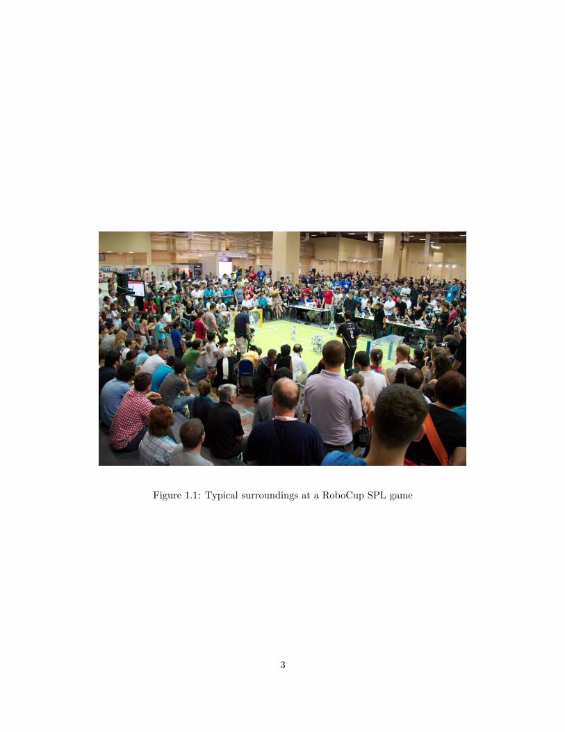
Figure 1.1: Typical surroundings at a RoboCup SPL game

3

Chapter 2

Background

The Kalman Filter (KF) and Monte-Carlo Particle Filter (PF) have grown to be the dominant

algorithms in robotic position tracking in RoboCup. A large body of literature exists on both

of these methodologies, so I will just briefly highlight some of the benefits and failings of each,

as well as some extensions to the core algorithms that can improve accuracy and performance.

2.1 Particle Filters

Particle Filters represent an approximation to the posterior using a finite number of randomly

drawn samples. In control updates each particle is treated separately, and moved in accordance

with the control function. In observation updates, particles are assigned a weight based on

how closely they match the observation, then samples are re-drawn with a probability equal to

their weight. This causes particles to move towards the mean of the posterior, whilst innately

retaining the ability to represent multiple modes. The B-Human RoboCup Standard Platform

League (SPL) team offers several modifications and optimisations to the PF that allow it to

run in a reasonable amount of time on the Nao, (Laue et al. [14]). The PF is an ‘any-time’

algorithm, its complexity is determined by the number of particles being used, this is traded

off by how accurately the posterior can be estimated. B-Human claim sufficient accuracy for

their purposes using only 100 particles to represent the posterior.

4

2.2 Kalman Filters

Kalman Filters represent the posterior as a normal distribution, which is parameterized as the

Gaussian function η(µ,Σ), where µ is the mean vector and Σ is the covariance matrix. The

primary benefit of using a KF over a PF is speed, KF updates run in linear time with respect

to the number of dimensions of the filter; furthermore its compact representation lends it

to distribution amongst a team of agents, however the basic KF algorithm does have some

pitfalls:

Since the KF is represented by a Gaussian function, it is inherently unimodal. When deal-

ing with ambiguous landmarks, multiple hypotheses for the robot’s position may be generated.

Providing a largely incorrect position hypothesis to a unimodal KF causes large errors in the

filter, which can be difficult to recover from, especially if the observation had a low variance.

To deal with this, the KF must be extended to the Multiple Hypothesis Filter (MHF) (Reid

[8]), which represents multiple hypotheses using a mixture of Gaussians with varying weights.

It can be shown that as the number of Gaussians used approaches infinity, it becomes possi-

ble to accurately approximate any posterior, but this is computationally intractable. In the

implementation described by (Sushkov [9]) on the Sony Aibo robot, 6 Gaussians were used.

When an update occurs, all 6 are cloned, and the update is applied to one clone, the weights

are then adjusted using a measurement likelihood function (Thrun et al. [15, pp 204,218-220]).

The 6 Gaussians with the highest weights are kept and the rest are discarded. This keeps

the number of models being tracked to a minimum, and has the nice side-effect of minimising

the impact of outlier observations. (Quinlan and Middleton [10]) suggest some alternative

heuristics for updating the weights in a mixture of Gaussians. Quinlan also points out that

the multi-modal KF implementation only requires 35% of the computational resources of a

PF with similar accuracy.

The other pitfall of Kalman filters is that the control and observation update equations

are assumed to be linear functions of the state. In practise this is often not the case, for

example a robot moving on a continuous circular path cannot be modelled using only a linear

5

function. To deal with realistic update functions, it is necessary to find an appropriate linear

approximation, two techniques have become popular for this purpose: the Extended Kalman

Filter (EKF) and the Unscented Kalman Filter (UKF) (Julier et al. [16]). The EKF operates

by using the derivatives of the update functions to find the line tangent to the update function

at the current mean. The resulting line is a linear function that can be applied directly using

the standard KF equations. The UKF can produce equal or better linearizations than the

EKF (Thrun et al. [see 15, pp. 69-70]), it operates by selecting sigma points at the mean,

and 1 standard deviation away in each direction in each dimension. The non-linear update

function is then evaluated at each of these sigma points to provide a linear function that can

be applied. The implementations described in (Sushkov [9]) and (Quinlan and Middleton

[10]) both use EKFs, however the same concepts can easily be adapted to a UKF.

2.3 Distributed Filtering

Distributed filters allow observations from other agents to be incorporated into the filter. The

most naive approach would be to have all agents transmit all observations, each of the receiving

agents can incorporate these observations after multiplying the uncertainty in the observation

by the internal uncertainty about the sender’s position (Roumeliotis and Rekleitis [12]). The

size of non-preprocessed data that would have to be sent across the network, however, makes

this approach infeasible, especially in the RoboCup SPL, where teams have strict bandwidth

restrictions. A more compact representation is necessary.

Panzieri et al. [13]; Roumeliotis and Bekey [11] explore methods for distributing Kalman

filters across a set of agents, focusing on the relative distances between agents. Panzieri relies

on a fixed agent as a point of reference to solve the global localization problem. Sushkov

[9] used a simplified version of these methods, modified for a team consisting of the 2006

RoboCup SPL robot, the Sony Aibo, which had very limited computing resources. In his

implementation, the ball acts as shared, unique landmark, and a state vector and covariance

matrix incorporating the ball and all team members’ positions are frequently transmitted.

6

2.4 Beyond rUNSWift 2010 Localisation

In 2010, (Ratter et al. [17]) used a hybrid PF/KF system. An expensive PF was run in the

initial state, or after detecting a kidnapped robot state. This PF would cull the large number

of hypotheses that could be generated from observations seen on a symmetrical field, until

a single and approximately correct estimate had been determined. At this point the more

nimble KF algorithm would take over, using the position of the final particle presented by the

PF as a seed.

As a single-modal filter, it operated in an ambiguous environment by choosing the hypoth-

esis that was most probable given the current state estimate. This approach easily allowed

errors to compound, falsely increasing the certainty in an incorrect hypothesis. For this reason

it was necessary to return to the PF quickly whenever observations that contradicted the KF

state estimate were detected.

The approach presented in Chapter 5 picks up where rUNSWift 2010’s localisation sys-

tem left off, using a similarly-structured Kalman filter, but introducing multiple-hypothesis

tracking to remove the need to switch into the Particle Filter mode. Additionally, manual

linearisations for new types of observations, including field lines and the centre circle, have

been added to the capabilities of the base Kalman filter.

7

Chapter 3

Underlying Infrastructure

The localisation systems described in this thesis form only one part of the complex software

package that rUNSWift uses to compete in the RoboCup SPL competition. This chapter will

outline how this system works as a whole, and where the localisation subsystem fits.

3.1 rUNSWift Software Architecture

The system architecture used by rUNSWift 2011 is heavily based on that developed by

rUNSWift 2010 Ratter et al. [17], but with several new improvements.

In order to streamline utilisation of the single CPU (a 500MHz AMD Geode) that the

Nao possesses, the processing pipeline is split into threads at each heavily IO-bound segment.

The core threads in the runswift executable are:

• Motion, which blocks on sensor readings from the robot’s body, and is responsible for

reading and writing sensor and joint angles.

• Perception, which blocks on reads from the camera device via Linux’s V4L2 imaging

subsystem, and is responsible for vision, localisation & behaviour.

• GCReceiver, which blocks on reading a network socket, processes and stores UDP broad-

cast messages received from the electronic referee.

8

• TeamReceiver, which similarly to the GCReceiver, processes UDP broadcast messages

received from other robots on the rUNSWift team.

• TeamTransmitter, which transmits information to the team at 5Hz, sleeping in between

transmission cycles.

Each of these threads, and the modules within them, share information with one another

using a central ‘blackboard’, which is globally accessible and supports the necessary synchroni-

sation primitives required for inter-thread messaging. In most cases, data that would result in

race conditions were they simultaneously read and written, is stored using the ‘double-buffer’

technique, as it allows for continuous nonblocking reads and writes of the blackboard.

Since the localisation module fits into the ‘perception’ thread, I will describe this in more

detail, aided by Figure 3.1.

Figure 3.1: Data flow in the rUNSWift Perception thread.

9

The first step of the perception thread is to update the transformation matrices that

allow for projects from image space to the ground plane and vice-versa, by loading the most

recent joint angle readings from the motion thread’s buffer on the blackboard. This later

allows vision to calculate the distance and heading to an object detected in an image, and

localisation and behaviour to calculate the expected position of a feature in the image from

robot-relative coordinates, should they require it.

The next step is reading a frame from one of the robot’s cameras, facilitated by the

V4L2 (Video for Linux) kernel driver. Detection algorithms then locate features such as goal

posts, balls, field edges, field lines, robots and other obstacles. The vision algorithms used by

rUNSWift 2011 are detailed by (Chatfield [18]; Kurniawan [19]; Harris [20]).

With these new visual observations in hand, the perception thread then runs the various

components of the localisation and world-modelling module. The self-position of the robot

is tracking using the algorithms described in Chapter 5, a separate Kalman filter variant

described by (Teh [21]) tracks the position and velocity of the ball relative to the robot,

opponents are tracking using a grid-based filtering method described by (Vance [22]), and

team-mates positions are recorded by transforming their self-localisation results which were

transmitted over the network, into self-relative coordinates.

Finally, the results of this world-model are stored in the blackboard, and the behaviour

routines are run. The behaviours used by rUNSWift have been implemented in a combination

of native C++ code, as well as the high-level Python scripting language. Implementing

behaviours in Python allowed for faster prototyping than would be possible using a compiled

language, because the Python interpreter allows classes to be re-loaded on the fly. The Linux

‘inotify’ module is used to detect changes in the filesystem and trigger a reloading of the

Python behaviours. The details of how the Python-C++ bridge was implemented can be

found in (Claridge [23]).

At the end of the perception cycle, an intention is published on the blackboard in the

form of an ‘action command’, which is picked up by the motion thread in its next cycle. The

10

motion thread then plans and actuates the execution of a walk, kick, head-movement, etc.

The details of the motion thread implementation can be found in (White [24]).

3.2 OffNao Simulator & Debugger

Another key element of the rUNSWift software package that allowed this localisation system

to be rapidly prototyped and developed was the OffNao application. OffNao is a C++ im-

plementation which links against the runswift executable and the Qt GUI toolkit libraries to

provide an interactive interface to the software the runs on the Nao.

OffNao serves two main purposes in the development of localisation algorithms. First,

is allows for the real-time streaming and recording of the robot’s internal state whilst it is

being used in our laboratory. This makes it possible to test and observe the outcomes of the

localisation algorithms being developed under realistic conditions. The ability to playback

these recordings frame-by-frame makes it easier to isolate problems in the robot’s software.

A screen-capture of OffNao streaming data from a Nao operating under game conditions can

be seen in Figure 3.2.

The second use of OffNao in developing localisation, is its role as a simulator. The locali-

sation tab, pictured in Figure 3.3, allows the operator to select which landmarks the simulated

robot will ‘observe’ by clicking on them. Each time an observation is made, the same localisa-

tion algorithms that would run on the robot are executed with this simulated data, allowing

the operator to observe the precise behaviour of the localisation routines under controlled

conditions. The simulator also allows for the adding of arbitrary amounts of Gaussian noise,

as well as systematic bais, which makes it possible to repeatably test the performance of the

filter under more difficult conditions.

When using the simulator, the creation, merging and destruction of modes is represented

by having a circle representing each mode’s mean on the field, and an ellipse representing that

mode’s covariance matrix. When testing algorithms that involve giving each mode a weight,

the weight is represented by how light or dark the robot circle appears to be.

11

Figure 3.2: Screen capture from Offnao when streaming from an active robot.

OffNao has proved to be an invaluable tool when developing localisation for RoboCup

2011, since by analysing individual updates, we have been able to detect and repair bugs

that may have gone unnoticed over a long period of time when only testing by observing the

robot’s behaviour.

12

Figure 3.3: Screen capture from the Offnao Localisation Simulator

13

Chapter 4

Unscented Kalman Filter Approach

As noted in Section 2.2, Kalman filters are a computationally cheap method of tracking a

probability distribution, by parametising that distribution as a Gaussian function. Previous

RoboCup teams, including rUNSWift, have had success utilising the Extended Kalman Filter,

which efficiently approximates the prediction and update functions of the linear Kalman filter

for non-linear functions, such as the relationship between a robot’s position and the distance

and heading to a fixed landmark. The Unscented Kalman Filter theoretically provides a better

approximation, since it uses a deterministic sampling technique (the unscented transform)

to select a minimal set of samples from the observation probability distribution, which can

then be propagated through a non-linear transformation function, to provide an approximate

mapping of the observation’s covariance in the state space being tracked. This automatic

linearisation method also does not require the calculation of any Jacobians, which can be a

complex problem in itself for some transition functions.

In order to determine if these benefits of the UKF could be applied to the RoboCup SPL

domain, we experimented with a UKF implementation for the Nao robot. In the end this

approach was abandoned prior to the competition due to a number of implementation issues,

and was instead replaced by the manual linearisation approach described in Chapter 5. This

chapter describes the progress made down the path of using a UKF for SPL localisation, and

14

the problems that were encountered along the way.

4.1 UKF Implementation

The implementation used was a C++ port of the ‘vanilla’ UKF algorithm described in detail

by (Thrun et al. [15, pp. 69-70]). The only elements unique to this implementation are the

observation-state transformation functions. Because several different types of observations

can be made by the vision system, each with varying dimensionalities, the prediction step was

implemented in a way that allowed sigma points for dynamically-sized observation vectors to

be provided, each with their own corresponding prediction function. As a result, not even the

code that performs the unscented transform, combining the sigma points to form a covariance

matrix, need be aware of the size of the observation vector. This was achieved by describing

each observation type in terms of a functor that is templated in the number of elements in

the observation vector, and the entire UKF algorithm being templated so that this parameter

could be passed through, in effect generating an entire unscented Kalman filter tuned for

each particular observation size, that applied its updates to the same shared state vector and

covariance matrix.

The following are the prediction functors used for each of the 3 observation types used dur-

ing the UKF experiments: distance-heading landmarks (single posts) Algorithm 1, distance-

heading-orientation landmarks (corners) Algorithm 2, and two-post observations Algorithm

3.

Each of these prediction functions captures the relationship between a type of observation

and the state space, by providing a prediction for where that observation should occur for a

given predicted state (the sigma point). This in turn allows the unscented transform to be

performed on the resulting prediction sigma points, whose distances to the actual observation

measures the uncertainty in each observation dimension. This residual covariance matrix is

then used to find the cross-covariance between state space and prediction space, leaving a

linear (gain) function in terms of the current state, which updates the state estimate and

15

Algorithm 1 Prediction functor for distance-heading observationstemplate <typename T, int n, int o>

class DHLandmarkPredictor : public PredictionFunctor<T, n, o> {

const AbsCoord landmark;

DHLandmarkPredictor(const AbsCoord &landmark_) : landmark(landmark_) {}

void operator()(Matrix<T, n+o, 1> sigma, Matrix<T, o, 1> &prediction) {

prediction[0] = sqrt(sqr(landmark.x() - sigma[0])

+ sqr(landmark.y() - sigma[1])) + sigma[3];

prediction[1] = atan2(landmark.y() - sigma[1], landmark.x()

- sigma[0]) - sigma[2] + sigma[4];

}

};

Algorithm 2 Prediction functor for distance-heading-orientation observationstemplate <typename T, int n, int o>

class DHOLandmarkPredictor : public PredictionFunctor<T, n, o> {

const AbsCoord landmark;

DHOLandmarkPredictor(const AbsCoord &landmark_) : landmark(landmark_) {}

void operator()(Matrix<T, n+o, 1> sigma, Matrix<T, o, 1> &prediction) {

prediction[0] = sqrt(sqr(landmark.x() - sigma[0])

+ sqr(landmark.y() - sigma[1])) + sigma[3];

prediction[1] = atan2(landmark.y() - sigma[1],

landmark.x() - sigma[0]) - sigma[2] + sigma[4];

prediction[2] = landmark.theta() - sigma[2] + sigma[5];

}

};

16

Algorithm 3 Prediction functor for two-post observationstemplate <typename T, int n, int o>

class TwoPostDHPredictor : public PredictionFunctor<T, n, o> {

AbsCoord left_post;

AbsCoord right_post;

void operator()(Matrix<T, n+o, 1> sigma, Matrix<T, o, 1> &prediction) {

prediction[0] = sqrt(sqr(left_post.x() - sigma[0])

+ sqr(left_post.y() - sigma[1])) + sigma[3];

prediction[1] = atan2(left_post.y() - sigma[1],

left_post.x() - sigma[0]) - sigma[2] + sigma[4];

prediction[2] = sqrt(sqr(right_post.x() - sigma[0])

+ sqr(right_post.y() - sigma[1])) + sigma[5];

prediction[3] = atan2(right_post.y() - sigma[1],

right_post.x() - sigma[0]) - sigma[2] + sigma[6];

}

};

covariance according to the regular linear Kalman filter algorithm.

4.2 Problems using the UKF

4.2.1 Numerical stability of the Cholesky decomposition

In order to select the best sigma points to use for predicting the observation, it is necessary

to calculate the magnitude of one standard deviation in each dimension of both state and

observation space. This is typically done by finding the matrix-square-root of the augmented

state-observation covariance matrix using the Cholesky decomposition.

While this approach worked well in the early stages of the filter’s lifetime, before the

estimates and predictions converge, the accuracy of the decomposition algorithm when used

on floating-point numbers comes into question when dealing with covariance matrices whose

values are of a very small magnitude. We frequently found that after several iterations of the

filter, when some of the dimensions (especially heading, which is measured in radians) begin

to have extremely small variances, the Cholesky decomposition routine used started produc-

ing resultant matrices that were non positive-definite, making them unusable as covariance

17

matrices. Experiments with several matrix libraries yielded similar results, and we are still

not certain what the underlying cause of the problem with the decomposition we are using is.

4.2.2 Impact of angles on the UKF

The second series of problems that were experienced with the UKF seem to be tied to the

modelling of the robot’s heading. Unlike regular scalar variables, the heading is bound be-

tween −π and π, necessitating a renormalisation of angles when they wrap around. However,

blindingly normalising angles causes more problems than it solves. During the generation

of sigma-points, the current heading estimate must have a value of one standard deviation

added to and subtracted from it, but if the magnitude of this deviation is greater than pi, it

is not possible to represent such a sigma point without wrapping back around towards the

mean. As a result the residual covariance of the observation may appear to be much larger

or smaller than it really is.

Several attempts were made to resolve this problem by scaling or normalising the angles

at various stages throughout the filter, but the impact of large values, especially during the

cross-covariance calculation step, is very difficult to reason about, and it is not clear which

elements of this matrix will eventually have an impact on the robot’s heading estimate and

which do not.

Further analysis may find a workaround in the UKF algorithm that deals with both of

these problems, but under the time constraints of preparing for the RoboCup competition,

we were unable to find such a solution. As a result, an alternative approach was attempted,

which yielded much more promising results, as described in the next chapter.

18

Chapter 5

Multi-modal Linear Kalman Filter

Approach

After obtaining unpromising results from my experiments using an Unscented Kalman Filter,

we decided to take a simpler approach. Because many types of observations, such as two posts

in a single frame, or a field line corner or T-junction, provide a finite set of hypotheses for

the absolute position of the robot on the field, they can be used directly by a linear Kalman

filter. For other observation types such as field edges or a single distance-heading to goal post

observation, an appropriate linearisation based on the current state estimate can be calculated

geometrically, removing the need for complex linearisation methods such as the EKF or UKF.

In this chapter I describe the localisation system used by rUNSWift 2011 that relies on these

‘hand-crafted’ transformations from observation space into state space, and a heuristic for

determining which modes should be updated in a multi-modal filter.

5.1 Hypothesis Generation from Observations

The follow sections describe the geometry used to estimate the robot state x, y, θ and variance

Σ for various observation types. This observations are split into two categories, ‘local’ and

19

‘global’. The ‘local’ updates are those that are based on observations that require manual

linearisation, using the current state estimate of the mode being updated. The ‘global’ ob-

servations stand on their own, and are not dependant on any existing state. In all cases the

observed state variances were estimated intuitively and tweaked based on performance when

the algorithm was tested on the robots.

5.1.1 Field-Edge Observations

Figure 5.1: Position estimate calculated using a field-edge observation

When generating a position estimate from a field edge, as seen in Figure 5.1 only elements

x, θ or y, θ are updated, based on which edge we are assuming the observation corresponds to.

The previous value of the other spacial dimension is kept from the existing mode, but with

an extremely large variance so that it does not create a false reinforcement of information not

20

present in the observation.

The variance of each variable is assumed to independent, so we have a diagonal covariance

matrix:

Σ =

Σx 0 0

0 Σy 0

0 0 Σθ

(5.1)

The variance in x or y is calculated according to the distance to the field edge, assuming

a 6◦ variance in the camera angle. The heading variance is assumed to be a constant. These

calculations are seen in Figure 5.2 and described in the follow equations:

φ = atan(edge distance

camera height) (5.2a)

Σx|y = (tan(φ+ 6◦) − tan(φ))2 (5.2b)

Σθ = (10◦)2 (5.2c)

5.1.2 Field-Corner & T-Junction Observations

Because corner and t-junction measurements have an orientation φ in addition to distance d

and heading θ, they can be used to calculate a finite set of position estimates without reference

to the current state estimate. Given an observation O and a landmark L, the robot position

R is given as:

Rx = d.cos(Lθ +Oφ) + Lx (5.3a)

Ry = d.sin(Lθ +Oφ) + Ly (5.3b)

Rθ = Lθ +Oφ −Oθ − π (5.3c)

21

Figure 5.2: Variance estimate calculated for a distance to an observation

5.1.3 Parallel Line Observations

The only places on the field where two parallel lines can be seen are in front of the goals at

either end of the field. Furthermore the goalie itself will never see this lines when in position

due to the field of view of the camera and the size of the goal box. As such, we can assume

that a robot seeing two parallel lines is in one of two symmetric positions, approaching the

goal box from towards the centre of the field. This update provides a very accurate close-range

estimate for a striker who is about to make a kick, and is too close to see both goal posts in

the same frame.

Given the distances and headings to two lines L1d, L1θ and L2d, L2θ, the x and θ values

22

of the corresponding robot position estimates are:

R1x =field− length

2−max(L1d, L2d) (5.4a)

R1θ =π − L1θ + L2θ

2(5.4b)

R2x =−field− length

2−max(L1d, L2d) (5.4c)

R2θ =−π − L1θ + L2θ

2(5.4d)

5.1.4 Two Post Observations

The same geometric methods described by (Ratter et al. [17]) were used to calculate the

position of the robot using two goal posts at various distances. The variances, Σ, are calculated

according to the same distance metric used for field-edges (see Sub-Section 5.1.1).

5.1.5 Post and T-Junction Observations

In developing this system, it was noticed that once within a meter of the goal posts, it

is very rare that an attacking robot will actually be able to see both the opponent’s goal

posts, making the crucial global updates that lock in a primary mode (see Section 5.4) very

rare. To compensate for this, a new combined observation type was added in this year’s filter.

Combining a single goal post, a single T-junction, and on what side of the post the T-junction

can be found, provides a unique pair of global landmarks.

With these two fixed-position landmark, the same geometry used for two post observations

(see Sub-Section 5.1.4) at close range, can be applied, resulting in extremely accurate position

estimates when within striking range of the opponent’s goal posts.

23

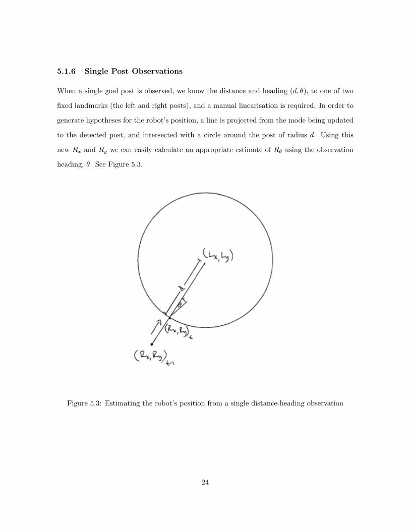
5.1.6 Single Post Observations

When a single goal post is observed, we know the distance and heading (d, θ), to one of two

fixed landmarks (the left and right posts), and a manual linearisation is required. In order to

generate hypotheses for the robot’s position, a line is projected from the mode being updated

to the detected post, and intersected with a circle around the post of radius d. Using this

new Rx and Ry we can easily calculate an appropriate estimate of Rθ using the observation

heading, θ. See Figure 5.3.

Figure 5.3: Estimating the robot’s position from a single distance-heading observation

24

5.1.7 Centre-Circle Observations

When a centre circle is detected without a line passing through it, the same calculations are

used as for a single goal post (Sub-Section 5.1.6), since we have only a distance and heading

to a landmark with known coordinates.

In the case that the centre line is also detected passing through the centre circle, an

additional orientation parameter is added to the observation, providing a complete global

position estimate as per Sub-Section 5.1.2, albeit with two hypotheses rather than one, due

to the circle’s symmetry.

5.2 Global and Local Update Functions

The traditional Kalman filer and Multi-Hypothesis tracking algorithms make several assump-

tions about the observations that will be passed into the filter, which do not hold in the

context of RoboCup SPL, in particular the assumption that no false-positive sensor readings

are passed into the filter causes great disruption to the standard algorithm.

In order to compensate for this, we have introduced an algorithm for selectively updating

or creating modes in the filter to minimise the disruption of a false positive observation.

Because of the different nature of ‘local’ and ‘global’ observations, one requiring an existing

mode as input and the other not, different algorithms are used for each of these update types.

In both cases the kalmanUpdate function is standard (Algorithm 4), except with an additional

mask parameter M , and its conjugate M , that allows a subset of the state dimensions to be

updated. So if we want to update x and θ, but not y, then:

M =

1 0 0

0 0 0

0 0 1

, M =

0 0 0

0 1 0

0 0 0

(5.5)

25

Algorithm 4 The linear Kalman filter update algorithm, instrumented to allow selectiveupdating of dimensions

function kalmanUpdate(mode, Σmode , hyp, Σhyp , M, M ):

// Calculate innovation and gain

hyp = M.hyp + M.modeinnov = hyp − modeΣinnov = M.Σhyp + Σmode

K = Σmode.Σ−1innov

// Mask off gain matrix

K = M.K// Update state and covariance

mode = mode + K.innovΣmode = Σmode − K.Σmode

Next is the algorithm to selectively update and create modes for a ‘global’ observation:

Algorithm 5 Algorithm to select which modes to update for a global observationgenerate all hypotheses for the observation

for each existing mode:

choose the hypothesis closest to this mode

if the distance between the closest hypothesis and this mode < threshold:

perform a kalmanUpdate on this mode with the closest hypothesis

mark this hypothesis as used

for each unused hypothesis:

generate a new mode from this hypothesis

Algorithm 5 has a number of useful properties:

• Each mode is updated at most once, with the hypothesis that is the best match

• False positive observations will not affect existing modes, due to the distance threshold

• New modes can be generated, helping the filter to leave a kidnapped-robot situation

after a single global update

Next is the algorithm to selectively update and create modes for a ‘local’ observation. In

this case we must generate hypotheses corresponding to every mode:

26

Algorithm 6 Algorithm to select which modes to update for a local observationfor each existing mode:

generate hypotheses for this mode:

if the closest matching hypothesis is < threshold_1 away:

perform a kalmanUpdate of this mode with the closest hypothesis

else:

increase the magnitude of this mode’s covariance matrix

for all unused hypotheses:

if the distance from the mode to the hypothesis is < threshold_2:

and if this hypothesis is not close to any other modes:

clone the mode

apply a kalmanUpdate to the clone with the hypothesis

Algorithm 6 has a number of useful properties:

• Each mode is updated at most once, with the hypothesis that is the best match

• New modes can be created, but only if the hypothesis would otherwise go unused

• False positive observations will not affect existing modes, due to threshold 1

• Absurd new modes will not be generated due to the (larger) threshold 2

5.3 Mode Merging and Removal

Although the algorithms in Section 5.2 minimise unnecessary creating of new modes, but first

trying to apply observations to existing modes, it is still possible that old modes that have not

received any new supporting observations (such as those generated from false-positive global

updates), are still left around unused for long periods of time.

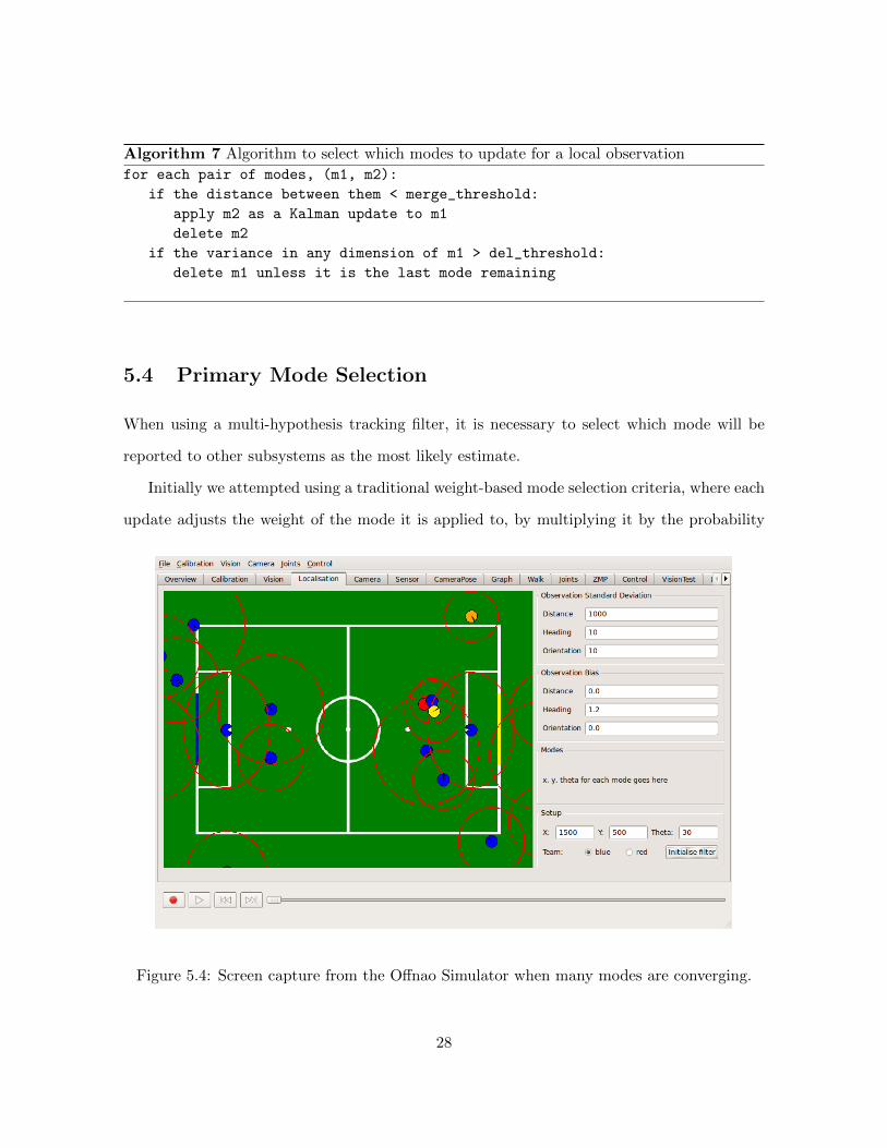
It is also common that a newly generated mode gravitates towards another existing mode,

as additional supporting evidence for that hypothesis is found. Resulting in several overlap-

ping modes (see Figure 5.4).

To resolve both of these problems, I present a simple algorithm for deciding when to merge

modes together and when to remove them entirely:

27

Algorithm 7 Algorithm to select which modes to update for a local observation

for each pair of modes, (m1, m2):

if the distance between them < merge_threshold:

apply m2 as a Kalman update to m1

delete m2

if the variance in any dimension of m1 > del_threshold:

delete m1 unless it is the last mode remaining

5.4 Primary Mode Selection

When using a multi-hypothesis tracking filter, it is necessary to select which mode will be

reported to other subsystems as the most likely estimate.

Initially we attempted using a traditional weight-based mode selection criteria, where each

update adjusts the weight of the mode it is applied to, by multiplying it by the probability

Figure 5.4: Screen capture from the Offnao Simulator when many modes are converging.

28

of that observation given that state estimate. The mode with the highest weight at the end

of each update cycle is reported as the primary mode.

In practise this did not work for us, because a robot looking at the same observation

for a couple of seconds, may have hundreds of repeated, similar observations, which due to

the symmetry of the field may be highly probable for several modes, subsequently weights

of those modes increase drastically, removing all weight of the remaining modes. The noise

in the observation then allows one of these symmetrical modes to gain dominance, resulting

in all other modes’ weights converging towards zero very rapidly. Once a mode’s weight is

near-zero, it is very difficult for it to ever become the dominant mode again, so a repeated and

slightly-offset observation would frequently remove a high quality mode from the mixture.

After several variations of probability-weight based mode selection were tested and failed

in turn, we adopted a much simpler heuristic for switching modes:

Whenever a global update takes place, and that global update has exactly one hypothesis

(not on any symmetrical global update, such as a field corner), then switch to the mode that

is the best match for that global update.

This would result in fairly infrequent mode switches, giving the filter a lot more stability

than the weight based methods, and because globally unique updates are rare (the only cases

for this are two-post and post-t-junction updates), it was unlikely that a false positive of this

type could occur. Once locked into a mode from a global update, the other local updates

would increase the accuracy the mode’s estimate, without affecting its rank as primary mode.

Other modes are still generated as per usual, but they do not take dominance until confirmed

by a globally unique update.

The downside to this approach is that a single false-positive global update, such as two

false-positive goal posts, can disrupt the filter enormously, but this was rare enough not to

be a significant problem.

Future work will involve devising a mode selection algorithm whose weight updates are

desensitised to repeated identical observations, resolving some of the problems stated above.

29

Chapter 6

Distributed Ball Tracking Approach

Because we are not using a unified filter across a team of robots, information about the location

of the ball must be manually combined when a robot is unable to find the ball individually.

This chapter describes the process used to estimate the ball position relative to a robot, given

that it cannot directly see the ball.

6.1 Transformation and Transmission

Each robot on the team prepares and transmits a structure via UDP broadcast at a rate of

5Hz. The structure contains the follow data elements:

• Team number

• Player number

• Robot-relative ball position & covariance matrix

• Robot’s primary mode from its localisation filter, including position & covariance matrix

• The number of frames since the ball was last seen

If a receiving robot wishes to know it’s robot-relative position to the ball, according to

the belief state of transmitting robot, the ball position is transformed from the robot-relative

30

coordinate space of the transmitting robot to absolute field coordinates, then back to robot-

relative coordinates, relative to the receiving robot.

6.2 Incapacitated Robot Detection

To avoid processing stale data, or data from robots whose world views have good reason to

be obscured or corrupted, we perform a test on each robot to see if it is ‘incapacitated’ before

using information in the buffer that contains data most recently received from that robot.

A robot is considered ‘incapacitated’ if any of the following conditions is true:

• The foot sensors report very low readings for more than 2 seconds (presumably the

robot has been picked up by the referee, or fallen over)

• The accelerometers indicate the robot’s vertical velocity is high enough for it to be

falling

• The y-axis gyroscope indicates an angle of inclination of more than 45◦

• The robot is performing a get-up routine

• The last network transmission was received more than 3 seconds ago (software, hardware

or network may have failed)

• The GameController indicates that the robot is penalised

Using this method has allowed us to avoid reprocessing stale data, and easily detect when

a robot’s transmissions are not to be trusted, increasing the reliability of any behaviours that

rely on information shared amongst the team, such as the find ball routine, described in the

next section.

31

6.3 The Find-Ball Routine

Because any one team member may be mislocalised in a way that would be disruptive to the

coalescing of the entire team’s absolute ball position estimates, for example if a robot has

selected an incorrect mode as the primary mode (see Section 5.4) in a position symmetrically

opposite to where it really is, we instead follow a strict hierarchy of which team mate’s

ball position estimate to believe first, and only move on to the next robot if the one being

considered does not know the location of the ball.

The find-ball behaviour algorithm that rUNSWift utilised at RoboCup 2011 is listed in

Algorithm 8.

Algorithm 8 Routine used by a robot trying to locate the ball on the fieldif ball was seen directly in last 3 seconds:

proceed to last local observation

else if we are checking the team ball:

turn in direction of team ball

if we reach the direction indicated by team ball, mark it as checked

else if we have no yet checked a team ball:

for player in (1..4):

if player != me

and player is not incapacitated

and player saw the ball in the last 3 seconds:

begin turning towards the ball coordinates indicated by player

else:

rotate in direction ball was last seen directly

You will notice that this algorithm always prioritises a ball observation from player 1 over

any other player. The reason for this is that player 1 (the goalie) is generally more reliably

localised, because it is rarely moving and has a clear view of most of the field.

32

Chapter 7

Results from RoboCup 2011

7.1 Ready Skill

Table 7.1 counts the number of times a robot was seen in the correct starting position, and out

of the correct starting position, at the end of a game’s ‘Ready’ state. This does not include

robots that were off the field at the time (due to hardware failure) or robots that could not

be seen in the field of view of the camera recording the game.

Being in the correct position indicates that the localisation system is reporting a primary

mode that closely approximates the true position of the robot. Being out of the position

indicates that the localisation system is reporting an incorrect location, or is indecisive about

the robot’s location.

7.2 Kick Direction

Table 7.2 counts the number of times a robot kicked in the correct direction during a game.

A kick is considered ‘correct’ if the direction the ball is going at the time of the kick would

have resulted in a goal being scored, had there been no obstacles, and the ball velocity and

direction remained constant. This case indicates the localisation system knows the robot’s

heading to a high degree of accuracy.

33

Table 7.1: Frequency of robot being in position after Ready state

Game In Position Out of Position

CMU Practice 5 1B-Human Practice 2 0L3M 13 1UTS-WrightEagle 7 2NTU 10 3Cerberus 18 1Nanyang 9 1HTWK 12 3

Total 76 12

A kick is ‘close’ if the direction is approximately correct, but would not have resulted in

a goal, this indicates the localisation system’s estimate is approximately correct, or there was

error in the actuation of the kick.

A kick is a ‘miss’ if the ball clearly goes in a direction other than that of the appropriate

goals, such as the ball going towards the outline, or towards the robot’s own goals. This

typically indicates the hypothesis being reported by localisation is a mode other than the one

that represents the robot’s true position.

34

Table 7.2: Frequency of robot kicking in the correct direction

Game Correct Close Miss

CMU Practice 1 1 0B-Human Practice 3 3 1L3M 5 3 1UTS-WrightEagle 8 2 4NTU 6 1 0Cerberus 11 0 0Nanyang 15 1 0HTWK 5 0 0

Total 54 11 6

Figure 7.1: Aftermath from a kick being placed in the correct direction

35

Chapter 8

Discussion of Results

As can be seen from the results tabulated in Chapter 7, the localisation system presented

here has succeeded in positioning the robot for kick-off situations in over 85% of cases, and

resulted in kicks being made in a correct or close direction in over 91% of cases, which is a

promising result but still leaves plenty of room for improvement.

Much of the success in these types of systems can be attributed not only to the algorithm

chosen, but to the approach used for testing and tuning the system. The selection of primary

modes, described in Section 5.4 in particular, may not be the most elegant approach to solving

the problem, but was a pragmatic solution that allowed the system to work in practise, in

most cases. Future work will involve improving the underlying systems so that such ‘tweaks’

are not necessary, but in the mean time this has proven to be an effective way of progressing

under the time-pressured conditions of RoboCup.

That said, there are clear failure modes that must be addressed. In the game against

UTS-WrightEagle, an unusually high number of kicks went in the wrong direction. Later

analysis of this game led us to believe that a false-positive blue goal post was being detected

in an onlooker’s jeans sitting on the side of the field. It corresponded with the T-junction

found on the side of the field, allowing a global update to take place in the filter, altering the

belief state so that the robot thought the blue goal was on the side half-way line. The drastic

36

influence of this single, but repeatable, false-positive instance, is one of the weaknesses of

the mode-selection algorithm used. It also reinforces the importance of designing vision and

other sensory systems to be weighted towards discarding false-positives rather than avoiding

false-negatives. In true following of the ‘garbage in, garbage out’ principle, we are yet to find

an algorithm that is truly resilient in the face of repeated false positive observations.

In other situations, the mode-selection algorithm chosen acquitted itself quite well. In

every case that the robot entered within 1.5 meters of the opponent’s goal post, a kick attempt

went in the correct direction, due to the ability to quickly switch into a mode that corresponded

with either a 2-post or a 1-post-and-T-junction observation that is often visible in that pose.

The addition of ‘local updates’ allowed these global estimates to be further refined, especially

in situations where the precision of the robot’s heading was of great importance, such as when

kicking.

Overall, we are very pleased with the results of the localisation sub-system used at this

year’s RoboCup. The consistent accuracy of robot placement at the start of a game allowed

us to effectively use strategies that rely on players being positioned accurately relative to one

another, and the heading accuracy throughout games was clearly crucial to the scoring of

goals, which enabled rUNSWift to proceed to the quarter-finals. I hope that this work will

provided a useful basis for future work on high performance parametric filters used in future

RoboCup competitions.

37

Chapter 9

Future Work

9.1 Observation Variance Modelling

The algorithms described in this thesis assume they are provided with an accurate represen-

tation of the variance of an observation. The x, y, and θ variances used, however, are just

best-guess estimates concocted by the author. Using a more rigorous approach to calculat-

ing observation variances would provide the filter with better information: it would be able

to converge more quickly when the information is accurate, and converge less quickly when

information may contain large (Gaussian) noise.

One such approach would be to use a ground-truth sensor system to correlate distance and

heading readings to landmarks with the true state. Such a system would not only be able to

measure the variance of such observations, but also any intrinsic biases introduced from the

robot’s kinematic chain. Once this model has been constructed, a lookup of the appropriate

variance parameters can be chosen when an observation is made, based on information such

as distance, position on the field, and type of landmark or feature being detected.

38

9.2 Robot Inertial Model

The Nao has a number of built-in sensors that are not currently being harnessed to aid in

localisation. In particular the gyroscope and accelerometer could be used to measure the

movement of the robot in real time, which may provide a more accurate process-update to

any sort of Bayesian filter. The current odometric model uses a dead-reckoning approach,

whereby the robot is assumed to have moved the distance and in the direction we tell it to.

This is clearly not the case when the robot slips on the carpet or makes contact with obstacles

such as other robots. There are also more subtle sources of error, such as the increased play

in joints over time as the robot heats up during extended use. None of these sources of error

can be accounted for without an inertial model that makes use of live sensor data.

9.3 Use of Visual Odometry

In addition to the inertial sensors built into the robot, by performing feature-matching or

some other sort of differential analysis over a series of consecutive image frames, it should

be possible to build a model of the robot’s movement based on what it can see. This is a

challenging problem due to the resource-limited nature of the Nao, and the complexity of the

associated computer vision problem; however, if solved, this could provide even more accurate

measurements of the robot’s movement than the poor-quality built in inertial sensors.

9.4 Multi-Agent Tracking

Since the Nao has a built in wireless card, it would be advisable to take advantage of this

capability of improve the accuracy of the team’s localisation. In 2006 (Sushkov [9]) presented

an implementation for the Sony Aibo robot with good results, a similar approach may be

adapted to the Nao to allow robots to localise based on the position of the ball as reported

by team-mates.

39

9.5 Mode Switching Algorithms

The mode-switching algorithm presented in Section 5.4 does not take into account the validity

of a particular mode over time, it only makes an instantaneous decision when a unique global

update takes place. While this has proven to be more robust to false-positive observations

than other methods attempted, a more reasonable approach might involve considering a mode

to be a ‘candidate’ for being the primary mode after a global update, but whether it takes

over should be a function of how worthwhile it is overall, determined by how well other

observations correspond. The development of such an algorithm would make the filter more

robust to outliers, and allow mode switching after several local updates when appropriate.

40

Chapter 10

Conclusions

In this thesis, we have show that by taking advantage of higher order knowledge about the

geometry of an agent’s environment, it is possible to efficiently, and with high reliability,

track the estimated position of that agent. Using an implementation of a linear Kalman filter,

whose input was generated through the manual linearisation of robot-relative observations,

and a mode-switching heuristic that is more robust to false-positive observations that previous

efforts using Kalman filters, we have been able to localise a Nao Humanoid Robot playing in

the 2011 RoboCup competition.

There remains broad scope to improve the accuracy and reliability of this system by

taking advantage of an entire team’s knowledge, using more sophisticated inertial models,

and variance models, and devising mode selection techniques that are robust to false-positive

observations.

As long as the RoboCup SPL takes place on the severely resource-limited hardware that it

is currently using, these more nimble Kalman filter based approaches will continue to offer the

distinct advantage over their heavyweight Particle Filter counterparts, that their runtime is

insubstantial compared to the other CPU intensive work that must be done, especially vision

processing. This is likely to continue to drive research in localisation towards lightweight

parametric filters like the Kalman filter.

41

Figure 10.1: Naos celebrating at the conclusion of RoboCup 2011

42

Bibliography

[1] RC. Robocup Official Website. http://www.robocup.org/.

[2] Rodney Brooks. Intelligence without representation. Artificial Intelligence, 47:139–159,

1991.

[3] Peter Stone and David McAllester. An architecture for action selection in robotic soccer.

In Proceedings of the Fifth International Conference on Autonomous Agents, 2001.

[4] Daniel Withopf and Martin Riedmiller. Effective methods for reinforcement learning in

large multi-agent domains. Information Technology Journal. 47 (2005) 5, 2005.

[5] Bernhard Hengst. Partial order hierarchical reinforcement learning. In Proceedings of

the 21st Australasian Joint Conference on Artificial Intelligence - AI-08, Auckland, New

Zealand, December 2008.

[6] Rudolf E. Kalman. A new approach to linear filtering and prediction problems. In

Transactions of the ASMEJournal of Basic Engineering, 1960.

[7] Nicholas Metropolis and S. Ulam. The monte carlo method. Journal of the American

Statistical Association, 44(247):pp. 335–341, September 1949. ISSN 01621459. URL

http://www.jstor.org/stable/2280232.

[8] Donald B. Reid. An algorithm for tracking multiple targets. In Decision and Control

including the 17th Symposium on Adaptive Processes, 1978 IEEE Conference on, vol-

ume 17, pages 1202 –1211, January 1978. doi: 10.1109/CDC.1978.268125.

43

[9] Oleg Sushkov. Robot Localisation Using a Distributed Multi-Modal Kalman Filter, and

Friends. Honours thesis, The University of New South Wales, 2006.

[10] Michael J. Quinlan and Richard H. Middleton. Multiple model kalman filters: A lo-

calization technique for robocup soccer. In Proceedings of the RoboCup International

Symposium 2009. Springer-Verlag, July 2009.

[11] S.I. Roumeliotis and G.A. Bekey. Distributed multirobot localization. Robotics and

Automation, IEEE Transactions on, 18(5):781 – 795, October 2002. ISSN 1042-296X.

doi: 10.1109/TRA.2002.803461.

[12] S.I. Roumeliotis and I.M. Rekleitis. Analysis of multirobot localization uncertainty prop-

agation. volume 2, pages 1763 – 1770 vol.2, October 2003. doi: 10.1109/IROS.2003.

1248899.

[13] S. Panzieri, F. Pascucci, and R. Setola. Multirobot localisation using interlaced extended

kalman filter. pages 2816 –2821, October 2006. doi: 10.1109/IROS.2006.282065.

[14] Tim Laue, Thijs Jeffry de Haas, Armin Burchardt, Colin Graf, Thomas Rofer, Alexander

Hartl, and Andrik Rieskamp. Efficient and reliable sensor models for humanoid soccer

robot self-localization. In Changjiu Zhou, Enrico Pagello, Emanuele Menegatti, Sven

Behnke, and Thomas Rofer, editors, Proceedings of the Fourth Workshop on Humanoid

Soccer Robots in conjunction with the 2009 IEEE-RAS International Conference on Hu-

manoid Robots, pages 22 – 29, Paris, France, 2009.

[15] Sebastian Thrun, Wolfram Burgard, and Dieter Fox. Probabilistic Robotics. MIT Press,

Cambridge, Massachusetts, September 2005.

[16] S. J. Julier, J. K. Uhlmann, and H. F. Durrant-Whyte. A new approach for filtering

nonlinear systems. In Proceedings of the American Control Conference, volume 3, pages

1628 – 1632, 1995.

44

[17] Adrian Ratter, Bernhard Hengst, Brad Hall, Brock White, Benjamin Vance, Claude Sam-

mut, David Claridge, Hung Nguyen, Jayen Ashar, Maurice Pagnucco, Stuart Robinson,

and Yanjin Zhu. rUNSWift Team Report 2010 Robocup Standard Platform League.

Only available online: http://www.cse.unsw.edu.au/~robocup/2010site/reports/

report2010.pdf, 2010.

[18] Carl Raymond Chatfield. rUNSWift 2011 Vision System: A Foveated Vision System for

Robotic Soccer. Honours thesis, The University of New South Wales, 2011.

[19] Jimmy Kurniawan. Multi-Modal Machine-Learned Robot Detection for RoboCup SPL.

Honours thesis, The University of New South Wales, 2011.

[20] Sean Harris. Efficient Feature Detection Using RANSAC. Honours thesis, The University

of New South Wales, 2011.

[21] Belinda Teh. Ball Modelling and its Applications in Robot Goalie Behaviours. Special

project report, The University of New South Wales, 2011.

[22] Benjamin Vance. Remote Control and Global Obstacle Detection for the RoboCup SPL.

Special project report, The University of New South Wales, 2011.

[23] David Gregory Claridge. Generation of Python Interfaces for RoboCup SPL Robots.

Taste of research report, The University of New South Wales, 2011.

[24] Brock Edward White. Humanoid Omni-Directional Locomotion. Honours thesis, The

University of New South Wales, 2011.

45

List of Figures

1.1 Typical surroundings at a RoboCup SPL game . . . . . . . . . . . . . . . . . . 3

3.1 Data flow in the rUNSWift Perception thread. . . . . . . . . . . . . . . . . . . 9

3.2 Screen capture from Offnao when streaming from an active robot. . . . . . . . 12

3.3 Screen capture from the Offnao Localisation Simulator . . . . . . . . . . . . . . 13

5.1 Position estimate calculated using a field-edge observation . . . . . . . . . . . . 20

5.2 Variance estimate calculated for a distance to an observation . . . . . . . . . . 22

5.3 Estimating the robot’s position from a single distance-heading observation . . . 24

5.4 Screen capture from the Offnao Simulator when many modes are converging. . 28

7.1 Aftermath from a kick being placed in the correct direction . . . . . . . . . . . 35

10.1 Naos celebrating at the conclusion of RoboCup 2011 . . . . . . . . . . . . . . . 42

46

List of Algorithms

1 Prediction functor for distance-heading observations . . . . . . . . . . . . . . . 16

2 Prediction functor for distance-heading-orientation observations . . . . . . . . . 16

3 Prediction functor for two-post observations . . . . . . . . . . . . . . . . . . . . 17

4 The linear Kalman filter update algorithm, instrumented to allow selective

updating of dimensions . . . . . . . . . . . . . . . . . . . . . . . . . . . . . . . . 26

5 Algorithm to select which modes to update for a global observation . . . . . . . 26

6 Algorithm to select which modes to update for a local observation . . . . . . . 27

7 Algorithm to select which modes to update for a local observation . . . . . . . 28

8 Routine used by a robot trying to locate the ball on the field . . . . . . . . . . 32

List of Tables

7.1 Frequency of robot being in position after Ready state . . . . . . . . . . . . . . 34

7.2 Frequency of robot kicking in the correct direction . . . . . . . . . . . . . . . . 35

47