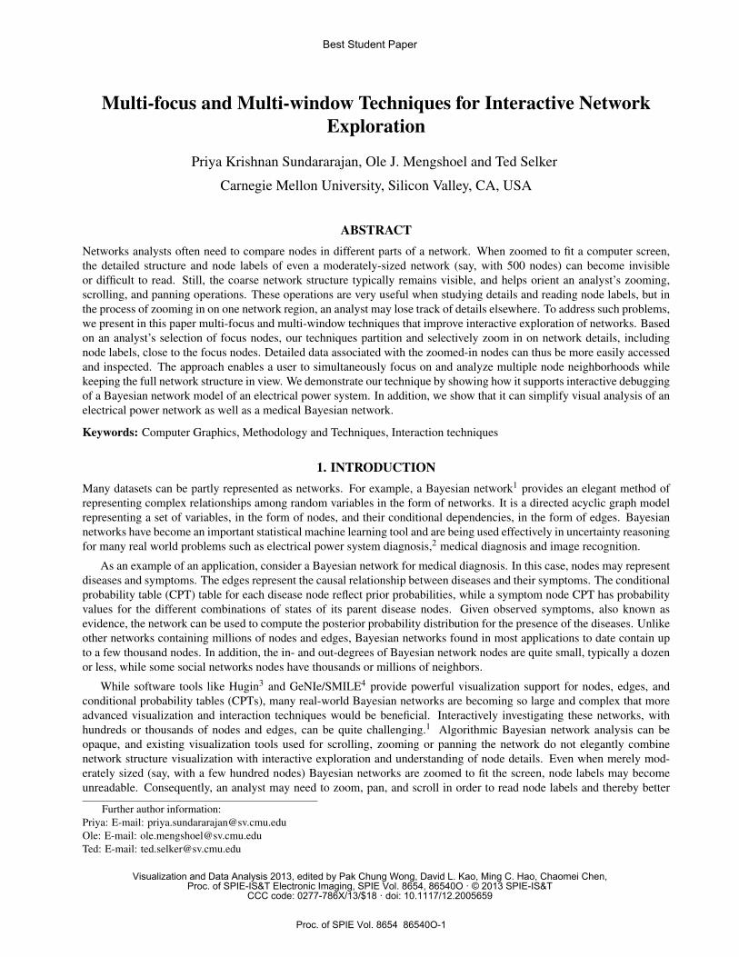
multi-focus and multi-window techniques for interactive ... and multi-window techniques for...

Multi-focus and Multi-window Techniques for Interactive NetworkExploration

Priya Krishnan Sundararajan, Ole J. Mengshoel and Ted Selker

Carnegie Mellon University, Silicon Valley, CA, USA

ABSTRACTNetworks analysts often need to compare nodes in different parts of a network. When zoomed to fit a computer screen,the detailed structure and node labels of even a moderately-sized network (say, with 500 nodes) can become invisibleor difficult to read. Still, the coarse network structure typically remains visible, and helps orient an analyst’s zooming,scrolling, and panning operations. These operations are very useful when studying details and reading node labels, but inthe process of zooming in on one network region, an analyst may lose track of details elsewhere. To address such problems,we present in this paper multi-focus and multi-window techniques that improve interactive exploration of networks. Basedon an analyst’s selection of focus nodes, our techniques partition and selectively zoom in on network details, includingnode labels, close to the focus nodes. Detailed data associated with the zoomed-in nodes can thus be more easily accessedand inspected. The approach enables a user to simultaneously focus on and analyze multiple node neighborhoods whilekeeping the full network structure in view. We demonstrate our technique by showing how it supports interactive debuggingof a Bayesian network model of an electrical power system. In addition, we show that it can simplify visual analysis of anelectrical power network as well as a medical Bayesian network.

Keywords: Computer Graphics, Methodology and Techniques, Interaction techniques

1. INTRODUCTIONMany datasets can be partly represented as networks. For example, a Bayesian network1 provides an elegant method ofrepresenting complex relationships among random variables in the form of networks. It is a directed acyclic graph modelrepresenting a set of variables, in the form of nodes, and their conditional dependencies, in the form of edges. Bayesiannetworks have become an important statistical machine learning tool and are being used effectively in uncertainty reasoningfor many real world problems such as electrical power system diagnosis,2 medical diagnosis and image recognition.

As an example of an application, consider a Bayesian network for medical diagnosis. In this case, nodes may representdiseases and symptoms. The edges represent the causal relationship between diseases and their symptoms. The conditionalprobability table (CPT) table for each disease node reflect prior probabilities, while a symptom node CPT has probabilityvalues for the different combinations of states of its parent disease nodes. Given observed symptoms, also known asevidence, the network can be used to compute the posterior probability distribution for the presence of the diseases. Unlikeother networks containing millions of nodes and edges, Bayesian networks found in most applications to date contain upto a few thousand nodes. In addition, the in- and out-degrees of Bayesian network nodes are quite small, typically a dozenor less, while some social networks nodes have thousands or millions of neighbors.

While software tools like Hugin3 and GeNIe/SMILE4 provide powerful visualization support for nodes, edges, andconditional probability tables (CPTs), many real-world Bayesian networks are becoming so large and complex that moreadvanced visualization and interaction techniques would be beneficial. Interactively investigating these networks, withhundreds or thousands of nodes and edges, can be quite challenging.1 Algorithmic Bayesian network analysis can beopaque, and existing visualization tools used for scrolling, zooming or panning the network do not elegantly combinenetwork structure visualization with interactive exploration and understanding of node details. Even when merely mod-erately sized (say, with a few hundred nodes) Bayesian networks are zoomed to fit the screen, node labels may becomeunreadable. Consequently, an analyst may need to zoom, pan, and scroll in order to read node labels and thereby better

Further author information:Priya: E-mail: [email protected]: E-mail: [email protected]: E-mail: [email protected]

Best Student Paper

Visualization and Data Analysis 2013, edited by Pak Chung Wong, David L. Kao, Ming C. Hao, Chaomei Chen,Proc. of SPIE-IS&T Electronic Imaging, SPIE Vol. 8654, 86540O · © 2013 SPIE-IS&T

CCC code: 0277-786X/13/$18 · doi: 10.1117/12.2005659

Proc. of SPIE Vol. 8654 86540O-1

understand the joint role of different network nodes in Bayesian network computations. Unfortunately, in the process ofzooming, panning, and scrolling, analysts may easily lose context. As an example, given a node of interest, it is hard tounderstand interactions with its children and parents if some of them are located far-off in the network layout. It is alsodifficult to keep values of the conditional probability tables (CPTs) in mind when studying and understanding zoomed-indetails. Our multi-focus and multi-window visualization techniques enable a user to better compare and analyze internaldetails of nodes in different parts of a network while retaining network context.

The fisheye technique5 seeks to enable zooming in on details while retaining context; it was introduced to address thefundamental visualization problem of finding a specific address node in a address book structure of AT&T employees.The fisheye technique maintains context and lets users study details, but allows focus on only one part of an informationstructure. In many cases, however, a user might need to compare multiple things in multiple parts of an informationstructure such as a network. Remembering the details of a previously studied zoomed node becomes a tedious memorytaxing and error prone activity as the number of nodes for comparison increases. This is the limitation of traditional singlefisheye techniques.

To overcome this limitation, as well as others, we formulate a number of design goals (DGs) that address our require-ments associated with interactive exploration and analysis of networks, in particular Bayesian networks. The goals assumethat zooming is being used. For the zooming algorithm, we integrate the previously stated goals6 and the suggestions fromBayesian experts. We hypothesized that the inherent complexity in Bayesian network representations could be overcomewith visualization tools that focus on comparing parts of the network and their contents.

DG1 Multi-focus zooming: Multiple focus nodes selected in different parts of the network should be zoomed simultane-ously, under user control, thus making their labels more readable regardless of their location in the network. Theprocess of zooming in and zooming out should be animated, to avoid hard to follow abrupt layout changes.

DG2 Topology maintenance: The continuity of layout adjustment should not challenge the user’s mental map of thestructure of the network, that is the topology, and the proximity relations of the nodes should be maintained.7

DG3 Focus nodes selection: The user should be able to determine which nodes to zoom by studying the details associatedwith a subset of nodes. A similar set of nodes such as current nodes in an electrical network or disease nodes in anmedical network, should be selectable by means of a search operation. A particular section of the network shouldalso be selectable by means of a group selection operation.

DG4 Scoped zooming: The zooming should be restricted to a region of interest or a partition, around a focus node toavoid distorting the whole network layout. A partition algorithm should intuitively decide on the region of interestaround the focus node for zooming. The set of nodes in the network should be partitioned accordingly. There is onepartition per focus node. With no focus node, there is one partition for all the nodes. The partitions around the focusnodes is used to localize the zooming effect within that region.

DG5 Dynamic partitioning: The partitioning algorithm should dynamically adjust the partitions as the user interactivelyadds or removes focus nodes for scoped zooming.

DG6 No ghost regions: After zooming, discontinuities or ‘ghost regions’ between the partitions should not exist.8

DG7 Context visibility: We consider both local and global context. For local context visibility, the user should be able tocontrol zooming to make the region surrounding the focus node more visible. For global context, the whole networkshould fit to the screen space and be visible during the user interactions. The user should still be able to controlzooming the whole network.

DG8 Label zooming: The user should be able to make the node labels of focused nodes bigger and more easily readable.The degree of zooming decreases as we move away from the focus node.

DG9 Data exploration: Users should be able to simultaneously open multiple detail windows associated with the networknodes. Depending on the type of network, the data-level windows should show node details such as CPTs, time-seriesgraphs or an individual’s bio-data for comparison or data analysis.


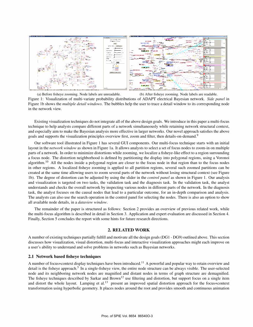
(a) Before fisheye zooming. Node labels are unreadable. (b) After fisheye zooming. Node labels are readable.Figure 1: Visualization of multi-variate probability distributions of ADAPT electrical Bayesian network. Side panel inFigure 1b shows the multiple detail windows. The bubbles help the user to trace a detail window to its corresponding nodein the network view.

Existing visualization techniques do not integrate all of the above design goals. We introduce in this paper a multi-focustechnique to help analysts compare different parts of a network simultaneously while retaining network structural context,and especially aim to make the Bayesian analysis more effective in larger networks. Our novel approach satisfies the abovegoals and supports the visualization principles overview first, zoom and filter, then details-on-demand.9

Our software tool illustrated in Figure 1 has several GUI components. Our multi-focus technique starts with an initiallayout in the network window as shown in Figure 1a. It allows analysts to select a set of focus nodes to zoom-in on multipleparts of a network. In order to minimize distortions while zooming, we localize a fisheye-like effect to a region surroundinga focus node. The distortion neighborhood is defined by partitioning the display into polygonal regions, using a Voronoialgorithm.10 All the nodes inside a polygonal region are closer to the focus node in that region than to the focus nodesin other regions. A localized fisheye zooming is applied to all partition regions, several such zoomed partitions can becreated at the same time allowing users to zoom several parts of the network without losing structural context (see Figure1b). The degree of distortion can be adjusted by using the slider in the control panel as shown in Figure 1. Our analysisand visualization is targeted on two tasks, the validation task and the diagnosis task. In the validation task, the analystunderstands and checks the overall network by inspecting various nodes in different parts of the network. In the diagnosistask, the analyst focuses on the causal nodes that lead to a particular outcome, for an in-depth comparison and analysis.The analysts can also use the search operation in the control panel for selecting the nodes. There is also an option to showall available node details, in a dataview window.

The remainder of the paper is structured as follows: Section 2 provides an overview of previous related work, whilethe multi-focus algorithm is described in detail in Section 3. Application and expert evaluation are discussed in Section 4.Finally, Section 5 concludes the report with some hints for future research directions.

2. RELATED WORKA number of existing techniques partially fulfill and motivate all the design goals (DG1 - DG9) outlined above. This sectiondiscusses how visualization, visual distortion, multi-focus and interactive visualization approaches might each improve ona user’s ability to understand and solve problems in networks such as Bayesian networks.

2.1 Network based fisheye techniquesA number of focus+context display techniques have been introduced.11 A powerful and popular way to retain overview anddetail is the fisheye approach.5 In a single-fisheye view, the entire node structure can be always visible. The user-selectednode and its neighboring network nodes are magnified and distant nodes in terms of graph structure are demagnified.The fisheye techniques described by Sarkar and Brown12 use filtering and distortion, but support focus on a single itemand distort the whole layout. Lamping et al.13 present an improved spatial distortion approach for the focus+contexttransformation using hyperbolic geometry. It places nodes around the root and provides smooth and continuous animation


as users click or drag nodes to read the focus point of the layout. This approach also distorts the whole layout for eachselection of focus point. In these techniques, some of our design goals are not satisfied, such as multi-focus zooming(DG1), topology maintenance (DG2), focus nodes selection (DG3), scoped zooming (DG4), dynamic partitioning (DG5)and data exploration (DG9). The design goals that are satisfied are continuity in layout (DG6), context visibility (DG7) andlabel zooming (DG8). Topology maintenance (DG2) is achieved in Furnas’s fisheye approach5 but not in the hyperbolicapproach.13

Sarkar et al.14 also investigated a two focus approach with orthogonal and polygonal stretching, where the simpleorthogonal distortion method maintains topological ordering of points (nodes maintain their left-of, above, etc. relation-ships), but the polygonal method does not. The zooming action is such that a user acts indirectly on the focus nodes througha ‘rubber sheet.’ This technique unfortunately produces violating the design goal, no ghost regions (DG6). Formella andKeller15 distort network layout outside a polygonal area to make space for zooming all nodes inside the circumscribedpolygon. This distortion mechanism does not scale to large networks as the user has to manually select the focus area byusing a rectangular selection. Both these techniques do not support dynamic partitioning (DG5).

A topological fisheye method16 precomputes coarsened graphs and renders the level of detail from the combined graphs,depending on the distance from one or more foci. This system supports more than one focus (DG1). The drawback, how-ever, is the computation involved in pre-computing the coarsened graphs, making it unsuitable for interactive exploration.Dynamic insets17 uses the connectivity of the graph to bring offscreen neighbours of on-screen nodes and their context intothe viewport as insets. Unfortunately, the entire structure of network is not visible in this technique violating DG7. Fenget. al. recently introduced a multi-focus+context technique18 for generating spatiotemporal coherent time-varying graphs.This technique utilizes a triangle mesh to partition the graph nodes and leverages this underlying mesh for constrainedmulti-focus+context visualization. This was achieved through formulating an energy function for optimized deformation.This approach supports design goals such as the topology maintenance (DG2), continuity in layout (DG6) and contextvisibility (DG7). The above approaches do not support design goals such as focus nodes selection (DG3), scoped zooming(DG4), dynamic partitioning (DG5), label zooming (DG8) and data exploration (DG9). Other zoom algorithms19 20 pro-vide more scalable multi-focus distortions, but without scoping of distortion, any focus change affects the entire networklayout in these approaches. Also, the user has no direct control over the sizes of nodes aside from opening or closing them.

As described, previous techniques do not support one of our design goal, namely scoped zooming (DG4), as they distortthe whole layout when rendering graphs at different levels. While the issue with distorting the whole layout is addressedby Reinhard et. al. in their improved fisheye zoom algorithm,6 it results in wasted screen space called ‘ghost regions,’ thusviolating DG6.

2.2 Tree based fisheye techniquesSeveral previous systems demonstrate focus+context techniques for tree visualization, like SpaceTree,21 which uses exten-sive zooming animation to help users stay oriented within its focus+context tree presentation. Unfortunately, this techniquedoes not support focus nodes selection (DG3), scoped zooming (DG4), dynamic partitioning (DG5), and creates ghost re-gions (DG6). The TreeJuxtaposer22 technique uses focus+context methods to support comparisons across hierarchicaldatasets. The technique also creates ghost regions (DG6). The reason is that this technique allows the user to do a rect-angular selection which usually gives rise to ‘ghost regions’. Also, these techniques require aggressive space constraintmethods if the nodes of comparison are far apart in the tree structure.

Tu and Shen present ‘balloon focus,’ a multi-focus context technique for treemaps. Their user study confirms that usersprefer the multi-focus treemaps to identify select players in a multi-year NBA dataset consisting of conferences, divisions,teams and player.23 While the treemaps provide good usage of the available space, network structure can be difficult toidentify.24 So this approach does not retain the topology of the network (DG2). Bayesian networks are in general not trees,making tree visualizations limiting.

2.3 Image based fisheye techniquesElmqvist et al.25 propose a new distortion technique that folds the intervening space to guarantee visibility of multiplefocus regions. The folds themselves show contextual information and support unfolding and paging interactions.25 Adrawback of this technique is the lack of user control over the scope of the focused regions. Non-linear magnification,26

pliable surfaces27 and compressed arc tangent graph algorithm,28 when applied to graphs, distort the labels within thezoomed areas. Such distortions make labels difficult to recognize or read (DG8). These techniques support multi-focus


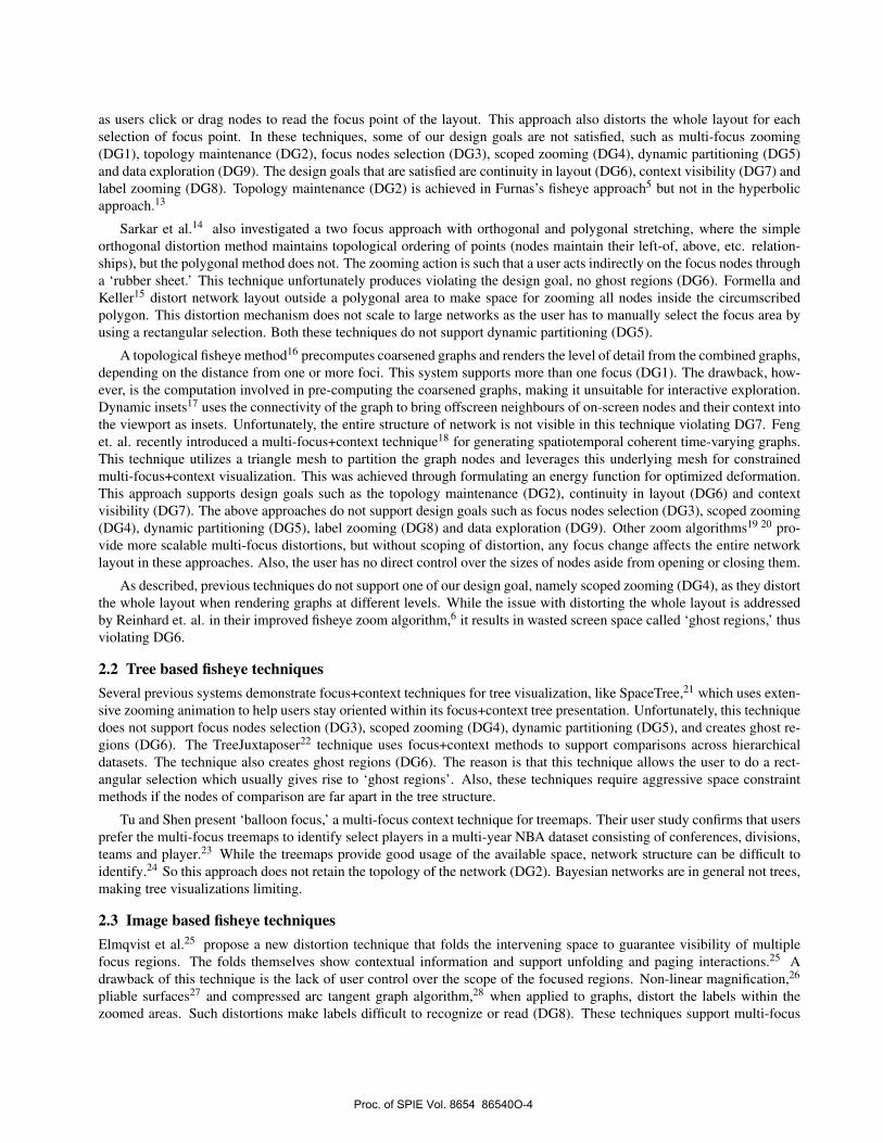
Figure 2: The diagram depicts the visulaization pipeline flow in our multi-focus algorithm. (a) The source data is loadedinto Prefuse data tables and converted to visualizable attributes in the visual abstraction. View transformation takes place inthree main steps: (b) before fisheye zooming; (c) partition generation; and (d) after fisheye zooming, also showing bubbleanchors.

zooming (DG1), topology maintenance (DG2), dynamic partitioning (DG5), no ghost regions (DG6), and context visibility(DG8). But they do not support focus nodes selection (DG3), scoped zooming (DG4) (as the whole layout is distorted foreach selection of focus point), label zooming (DG8) and data exploration (DG9).

3. MULTI-FOCUS ZOOMING AND MULTI-WINDOW TECHNIQUESOur multi-focus zooming algorithm helps to retain the network structure, thus limiting distortion to preserve the user’smental map of the Bayesian network. The distortion algorithm is independent of the layout algorithm and is defined as aseparate processing step on the layout of the graph. This allows for a modular organization of software29 and helped us toeasily understand, modify and reuse existing code to suit our visualization. However, care must be taken for the fisheyedistortion not to reduce readability of the display. To combat the negative aspect of distortion while giving an analystcontrol, we take the three steps shown in Figure 2:

• In the focus node selection step, the analyst selects a set of nodes for zooming. This can be done using a searchoperation over node labels or manually by selecting interesting nodes from the dataview window where all the detailwindows of the nodes are displayed.

• After selection of the focus nodes, regions around the focus nodes are created by the partition generation step, whichapplies an incremental algorithm that maintains a set of partitions that varies over time by insertion or deletion.30

This is shown in Figure 2c which has nine focus nodes and polygonal partitions. This second step also ensures thatall the nodes inside one partition are within that partition after distortion as shown in Figure 2d. This is done bymeasuring the maximum distance to move the node during distortion; the black lines as shown in Figure 4d denotesthe maximum distance to position the node so that it stays within the partition.

• The third step, fisheye zooming, distorts each partition as shown in Figure 2c. This results in zooming the focusnodes. For each focus node, the zooming gradually decreases as we approach the Voronoi edges of the partition.


The above three steps repeat as the new focus nodes are selected and zoomed. The process of zooming in our approachtherefore attempts to avoid the problems such as causing excessive distortions, excluding interactive rendering, excludingcomparing multiple parts of a graph, excluding identifiers being readable or excluding simultaneous exploration of contentsof nodes. Our technique is based on distorting the size and position of the label box based on its euclidean distances fromthe focus node. This helps to identify the focused node and its neighboring nodes.

Both Voronoi and rectangular partitioning approaches for a multi-focus technique have been proposed.31 We use theVoronoi partitioning approach32 as opposed to the traditional rectangular partitioning approach.31 This aids incrementalpartitioning (DG5) and continuous zooming layout (DG6) while preserving both structure and efficient use of space forarbitrary network structures. One benefit of the Voronoi approach is that it does not create ghost regions (DG6). Afterapplying the fisheye technique locally inside each polygon, the nodes near the sides of all polygons are compressed, topreserve layout continuity. Previous work has, to our knowledge, not combined the Voronoi and the fisheye algorithm formulti-focus zooming.

In addition to multi-focus, our approach is multi-window. The recent GraphPrism [10] shows graph measures in stackedhistograms and highlights nodes in a network based on selections in the histograms. We follow, and use multiple smallwindows to show more details such as the CPTs of the nodes. Having multiple windows with node detail information raisesthe question of maintaining a connection between a node and its details. We do this by means of ‘lines of bubbles’ (seeFigure 5). Like bubbles connecting thoughts to a character in a cartoon, bubbles act as anchors and connect nodes to theirdetails. Using these bubbles, the user can trace a detail window either in the side panel or floating, to its corresponding nodein the network view. The bubbles and the title bar of the detail window have the same color to clearly show their connection.We use an improved version of bubbles previously used,33 replacing the solid row of large dots with a progressivelyenlarged row of hollow bubbles. By using hollow bubbles, the user can now more easily see the network underneath thebubbles, see Figure 7 for solid bubbles and Figure 5 for hollow bubbles. We experimented with different bubble colorrepresentations, solid versus hollow bubbles and different sizes of the bubbles. We found that hollow colored bubbleswhich progressively increase in size as it reaches the side panel are more effective.

The pseudo-code of the multi-focus algorithm is shown in Figure 3; we now discuss each of the three steps in moredetail.

3.1 Step 1: Selection of focus nodesMany current visualization techniques mainly address how to display the data while the user’s primary concern, especiallyfor large datasets, is what is selected for display.5, 34 We provide several options as discussed in the below Section 3.1 tohelp users to study the details associated with each node to find the truly interesting nodes, satisfying design goal, focusnodes selection (DG3).

1. The user can study the details of the nodes (detail windows) such as the time-series graphs or the CPTs as shownin the dataview window (DG9). If an interesting behavior is found, the detail window can be selected so that thecorresponding node in the network window also gets selected.

2. In the network view, the detail windows can be viewed as a tooltip as the user hovers over a node. The detail windowassociated with a node can be anchored if the time-series graph or the CPT requires further inspection, see Figure 5.

3. A search operation can be used to select a set of nodes. This operation is useful, for example, when the user wantsto study all the current nodes or the voltage-sensor nodes in an electrical network, see Figure 7.

4. Rectangular selection allows the user to select a group of nodes in a particular region of the network. After selection,the detail windows associated with those nodes can be opened and studied in the side panel, see Figure 5.

5. Users can select neighboring nodes in a graph. The selected nodes can be zoomed and studied, see Figure 8 and 10.


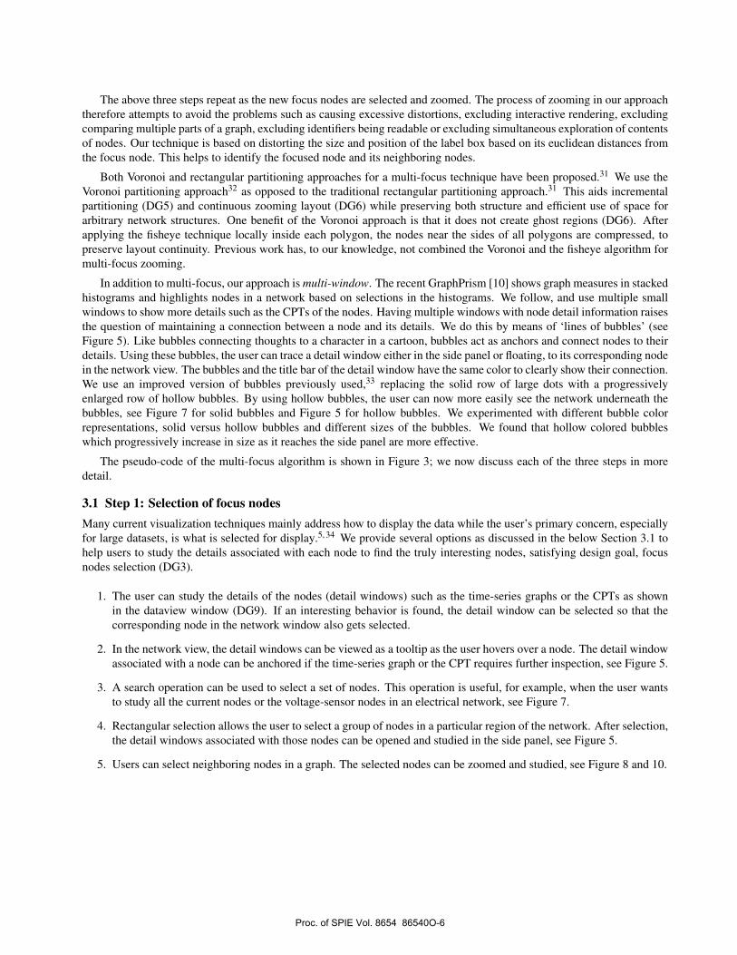
Algorithm 3.1: MULTI-FOCUS(NodeList)

procedure DRAWVORONOI(NodeList)comment: returns endpoints of the polygons

Fortune’s Voronoi algorithm is called to create the polygonsreturn (PolygonList)

procedure FISHEYEZOOMING(PolygonList,NodeList)comment: Apply fisheye distortion for each node

for polygon← PolygonList.next()

do

endPoints← polygon.getEnd pointS()for node← Graph.allnodes()

do

Ray casting is used to find if a node is inside the polygonif RayCasting(node) == true

then

NodesInPolygon← addNode(node)Get the intersectPoint of the nodeCompute DmaxApply arcTan fisheye distortion for the nodeCompute the new font size and position

return (NodesInPolygon)

main

Graph layout is rendered and wait for user operationif nodesSelected == true

then{

User can select nodes to start analysisNodeList← addNode(node)

PolygonList← DRAWVORONOI(NodeList)NodesInPolygon← FISHEYEZOOMING(PolygonList,NodeList)

Figure 3: Pseudocode for multi-focus algorithm. The DrawVoronoi function takes the focus nodes (Nodelist) as inputsand outputs the endpoints of the polygons (PolygonList) for each focus node. The FisheyeZooming function takes thePolygonList and the NodeList as inputs and returns the distorted nodes (NodesInPolygon).

3.2 Step 2: Partition GenerationAfter selecting a set of focus nodes, a bounded region around each of the focus node should be automatically selected bythe partitioning algorithm. The zooming algorithm is applied inside this region.

We experimented with a variety of rectangular partitioning approaches but found them causing discontinuities.31 TheVoronoi algorithm30 can satisfy several design goals (DG4, DG5 and DG6); its works by dividing the display area into npolygonal regions, given n node selections. This algorithm is based on the principle that any node in the region will benearer to the focus node in that region than to any focus nodes in neighboring regions.

When a node becomes a focus node, a partitioning algorithm30 is applied to that node and neigboring existing focusnodes to generate a new polygon, showing the incremental aspect of the algorithm. We apply the local fisheye to a boundedarea by retrieving the corner co-ordinates of the region and updating the display accordingly. Each node in the graph ischecked to see if it is present in the selected nodes’ partitioned area using a ray casting technique. ∗ Only those nodes inthe selected nodes’ partitioned area undergoes the fisheye distortion.

3.3 Step 3: Fisheye ZoomingThe analyst may want study the focus nodes in each partition. To do this, he may zoom-in on the focus nodes and thenearby nodes in the partitions. A local fisheye effect does this; the selected node is zoomed in and the size of the nearbynodes increases. We minimize the traditional fisheye effect that distorts the whole layout by localizing the fisheye effectwithin a partition. The user-selected node and its nearby nodes are magnified (DG7); the size of the nearby nodes decreaseby the arctan of the distance from the focus as they reach the edge of the polygonal partition providing a continuous layout.∗http://www.ecse.rpi.edu/Homepages/wrf/Research/Short_Notes/pnpoly.html


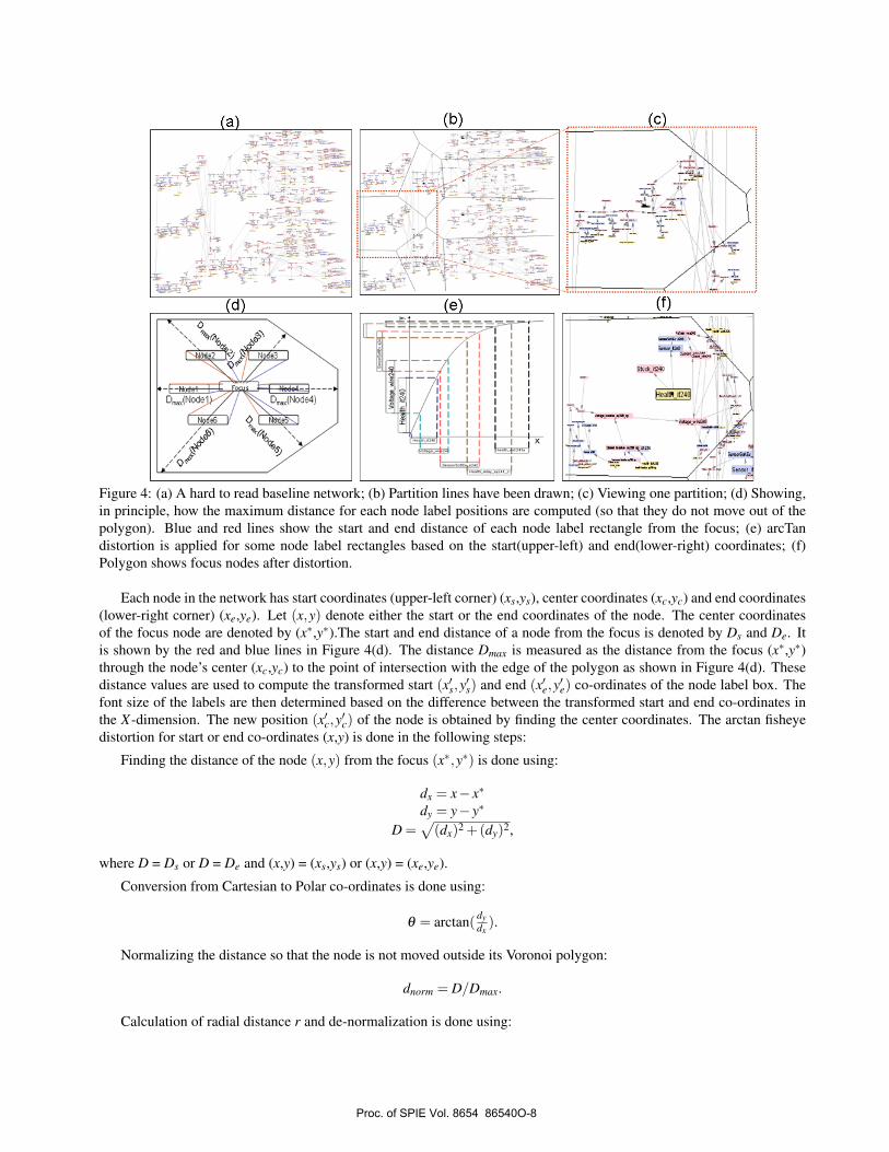
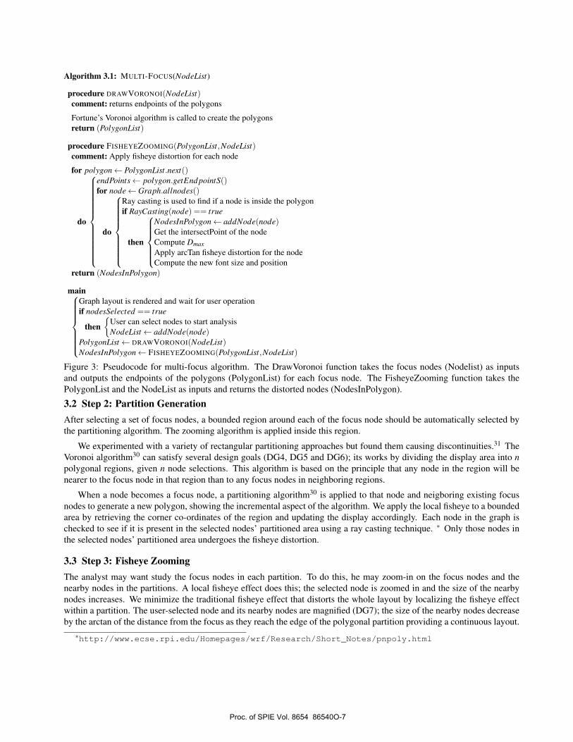
Figure 4: (a) A hard to read baseline network; (b) Partition lines have been drawn; (c) Viewing one partition; (d) Showing,in principle, how the maximum distance for each node label positions are computed (so that they do not move out of thepolygon). Blue and red lines show the start and end distance of each node label rectangle from the focus; (e) arcTandistortion is applied for some node label rectangles based on the start(upper-left) and end(lower-right) coordinates; (f)Polygon shows focus nodes after distortion.

Each node in the network has start coordinates (upper-left corner) (xs,ys), center coordinates (xc,yc) and end coordinates(lower-right corner) (xe,ye). Let (x,y) denote either the start or the end coordinates of the node. The center coordinatesof the focus node are denoted by (x∗,y∗).The start and end distance of a node from the focus is denoted by Ds and De. Itis shown by the red and blue lines in Figure 4(d). The distance Dmax is measured as the distance from the focus (x∗,y∗)through the node’s center (xc,yc) to the point of intersection with the edge of the polygon as shown in Figure 4(d). Thesedistance values are used to compute the transformed start (x′s,y

′s) and end (x′e,y

′e) co-ordinates of the node label box. The

font size of the labels are then determined based on the difference between the transformed start and end co-ordinates inthe X-dimension. The new position (x′c,y

′c) of the node is obtained by finding the center coordinates. The arctan fisheye

distortion for start or end co-ordinates (x,y) is done in the following steps:

Finding the distance of the node (x,y) from the focus (x∗,y∗) is done using:

dx = x− x∗

dy = y− y∗

D =√(dx)2 +(dy)2,

where D = Ds or D = De and (x,y) = (xs,ys) or (x,y) = (xe,ye).

Conversion from Cartesian to Polar co-ordinates is done using:

θ = arctan( dydx).

Normalizing the distance so that the node is not moved outside its Voronoi polygon:

dnorm = D/Dmax.

Calculation of radial distance r and de-normalization is done using:


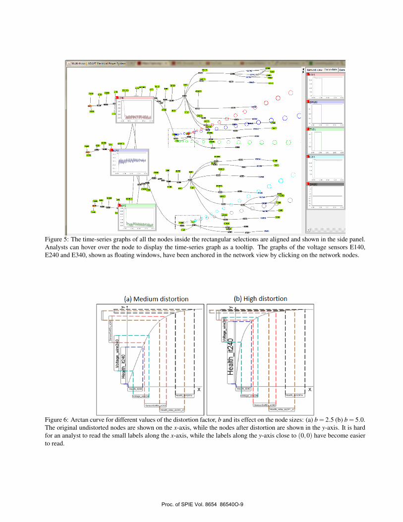
Figure 5: The time-series graphs of all the nodes inside the rectangular selections are aligned and shown in the side panel.Analysts can hover over the node to display the time-series graph as a tooltip. The graphs of the voltage sensors E140,E240 and E340, shown as floating windows, have been anchored in the network view by clicking on the network nodes.

Figure 6: Arctan curve for different values of the distortion factor, b and its effect on the node sizes: (a) b = 2.5 (b) b = 5.0.The original undistorted nodes are shown on the x-axis, while the nodes after distortion are shown in the y-axis. It is hardfor an analyst to read the small labels along the x-axis, while the labels along the y-axis close to (0,0) have become easierto read.


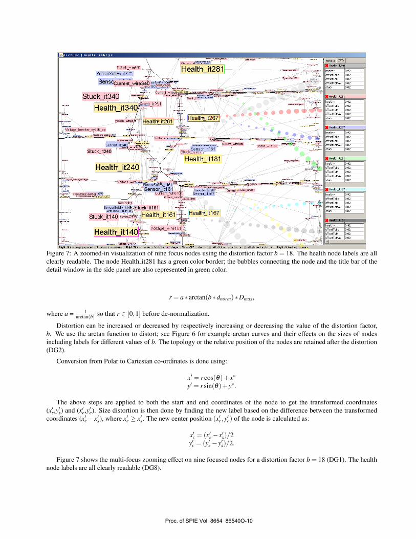
Figure 7: A zoomed-in visualization of nine focus nodes using the distortion factor b = 18. The health node labels are allclearly readable. The node Health it281 has a green color border; the bubbles connecting the node and the title bar of thedetail window in the side panel are also represented in green color.

r = a∗ arctan(b∗dnorm)∗Dmax,

where a = 1arctan(b) so that r ∈ [0,1] before de-normalization.

Distortion can be increased or decreased by respectively increasing or decreasing the value of the distortion factor,b. We use the arctan function to distort; see Figure 6 for example arctan curves and their effects on the sizes of nodesincluding labels for different values of b. The topology or the relative position of the nodes are retained after the distortion(DG2).

Conversion from Polar to Cartesian co-ordinates is done using:

x′ = r cos(θ)+ x∗

y′ = r sin(θ)+ y∗.

The above steps are applied to both the start and end coordinates of the node to get the transformed coordinates(x′s,y

′s) and (x′e,y′e). Size distortion is then done by finding the new label based on the difference between the transformed

coordinates (x′e− x′s), where x′e ≥ x′s. The new center position (x′c,y′c) of the node is calculated as:

x′c = (x′e− x′s)/2y′c = (y′e− y′s)/2.

Figure 7 shows the multi-focus zooming effect on nine focused nodes for a distortion factor b = 18 (DG1). The healthnode labels are all clearly readable (DG8).


4. APPLICATIONOur novel multi-focus technique is implemented using the Prefuse framework.35 ADAPT Bayesian network as well as othernetworks have been visualized. Figure 9 † shows the usage of the multi-focus technique in detecting faulty components inan electrical power system. Figure 10 shows the Munin2 Bayesian network with 1003 nodes where the children of a node(Proximal Myopathy) are zoomed using our multi-focus technique.

4.1 Bayesian NetworksThe ADAPT Bayesian network, which can be used for automatic fault diagnosis,2 models an electrical power network thatis representative of those found in aerospace vehicles. ADAPT has capabilities for power storage, distribution, and con-sumption, and contains batteries, electromechanical relays, circuit breakers, and different kinds of loads, such as pumps,fans, and light bulbs. Each component in ADAPT is modeled as a set of nodes. Health nodes (H) and the evidence (e) areof particular interest. The health nodes serve as the query variables, e.g. whether a component is defective or not, and theevidence nodes serve as the input variables, e.g. a command such as closing a relay to allow current from the battery toflow to the load. As an example fault scenario,2 suppose that e = {CommandRelay = cmdClose, SensorCurrent = readCur-rentLo, SensorVoltage = readVoltageHi, SensorTouchSensor = readClosed}. This gives argmaxP(H | e)= {HealthBattery= healthy, HealthLoad = healthy, HealthCurrent = stuckCurrentLo, HealthVoltage = healthy}. In this scenario, given theevidence of the command and sensor readings, the current flows from the battery to the load as both of them are healthy,also the voltage sensor is healthy. So the defective component is the current sensor which reads low instead of high.

A visualization of the ADAPT network in which labels are hard to read (and with no distortion) is shown in Figure1a. The network consists of 671 nodes and 790 edges. The font size of the labels is the same for all the nodes. With thenetwork fit to screen, as it is here, it is impossible to read these labels on the computer screen making it extremely difficultto understand, validate or edit the Bayesian network. Using our software, the analyst interacts with the graph by changingthe position of focus. The focus nodes that have been zoomed, will use a larger font for labels than their neighboring nodesas shown in Figure 7. It is now possible to read the node labels for the focus nodes and the nodes close to them. In general,multi-focus selection is used to make the labels readable and for comparing various nodes to explore their differences andsimilarities. The side panel in Figure 7 shows detailed information about the nodes, specifically the conditional probabilitytables, for further comparison and analysis.33 The bubbles help the user to trace the detail window to its correspondingnode in the network view.

4.2 Analytical TasksSeveral problem solving tasks can be performed with a Bayesian network; we consider the validation and the diagnosistasks.

4.2.1 Validation Task

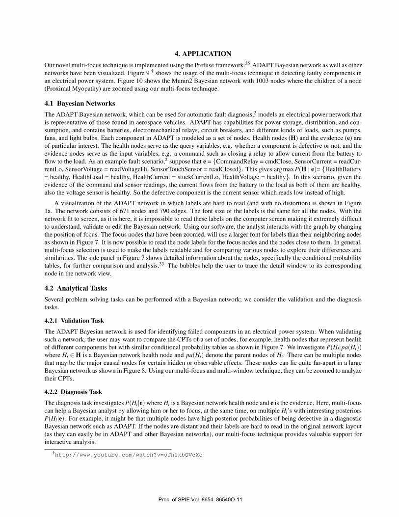
The ADAPT Bayesian network is used for identifying failed components in an electrical power system. When validatingsuch a network, the user may want to compare the CPTs of a set of nodes, for example, health nodes that represent healthof different components but with similar conditional probability tables as shown in Figure 7. We investigate P(Hi|pa(Hi))where Hi ∈ H is a Bayesian network health node and pa(Hi) denote the parent nodes of Hi. There can be multiple nodesthat may be the major causal nodes for certain hidden or observable effects. These nodes can lie quite far-apart in a largeBayesian network as shown in Figure 8. Using our multi-focus and multi-window technique, they can be zoomed to analyzetheir CPTs.

4.2.2 Diagnosis Task

The diagnosis task investigates P(Hi|e) where Hi is a Bayesian network health node and e is the evidence. Here, multi-focuscan help a Bayesian analyst by allowing him or her to focus, at the same time, on multiple Hi’s with interesting posteriorsP(Hi|e). For example, it might be that multiple nodes have high posterior probabilities of being defective in a diagnosticBayesian network such as ADAPT. If the nodes are distant and their labels are hard to read in the original network layout(as they can easily be in ADAPT and other Bayesian networks), our multi-focus technique provides valuable support forinteractive analysis.

†http://www.youtube.com/watch?v=oJh1kbQVcXc


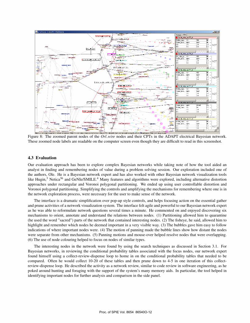
Figure 8: The zoomed parent nodes of the Orl wire nodes and their CPTs in the ADAPT electrical Bayesian network.These zoomed node labels are readable on the computer screen even though they are difficult to read in this screenshot.

4.3 EvaluationOur evaluation approach has been to explore complex Bayesian networks while taking note of how the tool aided ananalyst in finding and remembering nodes of value during a problem solving session. Our exploration included one ofthe authors, Ole. He is a Bayesian network expert and has also worked with other Bayesian network visualization toolslike Hugin,3 Netica36 and GeNIe/SMILE.4 Many features and algorithms were explored, including alternative distortionapproaches under rectangular and Voronoi polygonal partitioning. We ended up using user controllable distortion andVoronoi polygonal partitioning. Simplifying the controls and amplifying the mechanisms for remembering where one is inthe network exploration process, were necessary for the user to make sense of the network.

The interface is a dramatic simplification over pop-up style controls, and helps focusing action on the essential gatherand prune activities of a network visualization system. The interface felt agile and powerful to our Bayesian network expertas he was able to reformulate network questions several times a minute. He commented on and enjoyed discovering sixmechanisms to orient, annotate and understand the relations between nodes. (1) Partitioning allowed him to quarantine(he used the word ”sacred”) parts of the network that contained interesting nodes. (2) The fisheye, he said, allowed him tohighlight and remember which nodes he deemed important in a very visible way. (3) The bubbles gave him easy to followindications of where important nodes were. (4) The motion of panning made the bubble lines show how distant the nodeswere separate from other mechanisms. (5) Panning motions and mouse-over helped resolve nodes that were overlapping.(6) The use of node colouring helped to focus on nodes of similar types.

The interesting nodes in the network were found by using the search techniques as discussed in Section 3.1. ForBayesian networks, in reviewing the conditional probability tables associated with the focus nodes, our network expertfound himself using a collect-review-dispense loop to home in on the conditional probability tables that needed to becompared. Often he would collect 10-20 of these tables and then prune down to 4-5 in one iteration of this collect-review-dispense loop. He described the activity as a network review, similar to code review in software engineering, as hepoked around hunting and foraging with the support of the system’s many memory aids. In particular, the tool helped inidentifying important nodes for further analysis and comparison in the side panel.


Figure 9: Time-series graphs of the zoomed sensor nodes in the ADAPT electrical power network. The node labels andtheir time-series graphs are readable for further analysis. The time-series graphs around the node CB180 show a drop intheir reading, suggesting that the component CB180 is faulty.

5. DISCUSSION AND FUTURE WORKDistortion such as fisheye views can increase the ability to keep context visible. Multi-focus approaches improve visualanalysis by allowing comparison of different parts of a network, providing analysts with a collect-review-dispense an-alytical task scenario. Our system generates distortion boundaries which can reduce global distortion, reducing visualcomparison challenges. In particular, our technique allows an analyst to interactively bring important parts of a network‘forward’ by selectively zooming in, to be compared both structurally in the network and in a multi-window semanticdisplay.33 Our system can be used to create over a dozen focus partitions.

This system gives simultaneous multi-focus and multi-window zooming capability that enables improved interactivevisual exploration of Bayesian networks. In case of a failure in an electrical circuit, the user may want to find the faultycomponent. For this, a deeper analysis of each of the component is required. Using the multi-focus technique, similarcomponents like voltage or current sensors, can be zoomed; using the multi-window technique their internal readings canbe studied. The multiple windows which contain detailed data can be floating or aggregated in side panel. The side panelis designed to align and compare internal readings of multiple selected nodes. If there is any sudden drop or rise in thereadings in any of the components, then it can be diagnosed further.

The multi-focus with the multi-window views shown in this paper promises to improve completion accuracy in networkanalysis; we hope to validate this in future work. We have used our technique in electrical networks (Figure 9), Bayesiannetworks (Figure 10) and even on social networks. This paper pushes for adding techniques to the arsenal of ways toallow users to better view large networks and analyze their complex problems. Analytics and reasoning are being done onincreasingly complex datasets. This paper demonstrates improvements towards and calls for future work on systems thatintegrates scalable user interactivity into comparing parts and internal semantics of large-scale networks.


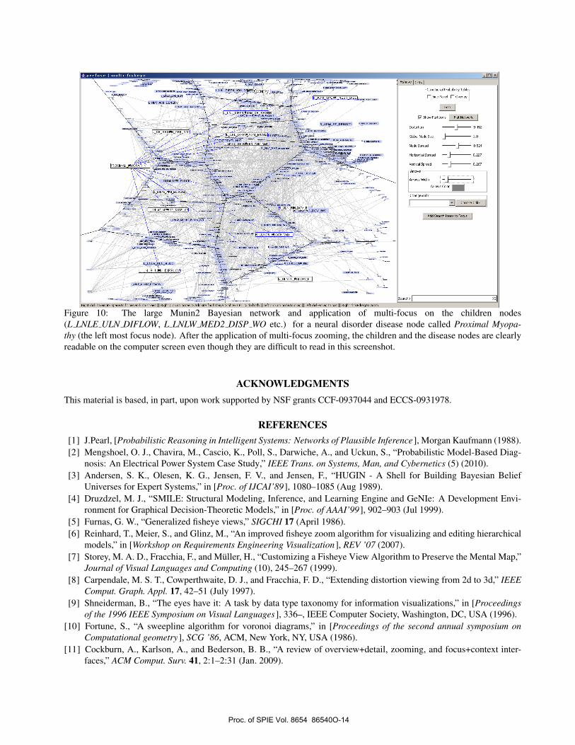
Figure 10: The large Munin2 Bayesian network and application of multi-focus on the children nodes(L LNLE ULN DIFLOW, L LNLW MED2 DISP WO etc.) for a neural disorder disease node called Proximal Myopa-thy (the left most focus node). After the application of multi-focus zooming, the children and the disease nodes are clearlyreadable on the computer screen even though they are difficult to read in this screenshot.

ACKNOWLEDGMENTSThis material is based, in part, upon work supported by NSF grants CCF-0937044 and ECCS-0931978.

REFERENCES[1] J.Pearl, [Probabilistic Reasoning in Intelligent Systems: Networks of Plausible Inference], Morgan Kaufmann (1988).[2] Mengshoel, O. J., Chavira, M., Cascio, K., Poll, S., Darwiche, A., and Uckun, S., “Probabilistic Model-Based Diag-

nosis: An Electrical Power System Case Study,” IEEE Trans. on Systems, Man, and Cybernetics (5) (2010).[3] Andersen, S. K., Olesen, K. G., Jensen, F. V., and Jensen, F., “HUGIN - A Shell for Building Bayesian Belief

Universes for Expert Systems,” in [Proc. of IJCAI’89], 1080–1085 (Aug 1989).[4] Druzdzel, M. J., “SMILE: Structural Modeling, Inference, and Learning Engine and GeNIe: A Development Envi-

ronment for Graphical Decision-Theoretic Models,” in [Proc. of AAAI’99 ], 902–903 (Jul 1999).[5] Furnas, G. W., “Generalized fisheye views,” SIGCHI 17 (April 1986).[6] Reinhard, T., Meier, S., and Glinz, M., “An improved fisheye zoom algorithm for visualizing and editing hierarchical

models,” in [Workshop on Requirements Engineering Visualization], REV ’07 (2007).[7] Storey, M. A. D., Fracchia, F., and Muller, H., “Customizing a Fisheye View Algorithm to Preserve the Mental Map,”

Journal of Visual Languages and Computing (10), 245–267 (1999).[8] Carpendale, M. S. T., Cowperthwaite, D. J., and Fracchia, F. D., “Extending distortion viewing from 2d to 3d,” IEEE

Comput. Graph. Appl. 17, 42–51 (July 1997).[9] Shneiderman, B., “The eyes have it: A task by data type taxonomy for information visualizations,” in [Proceedings

of the 1996 IEEE Symposium on Visual Languages], 336–, IEEE Computer Society, Washington, DC, USA (1996).[10] Fortune, S., “A sweepline algorithm for voronoi diagrams,” in [Proceedings of the second annual symposium on

Computational geometry], SCG ’86, ACM, New York, NY, USA (1986).[11] Cockburn, A., Karlson, A., and Bederson, B. B., “A review of overview+detail, zooming, and focus+context inter-

faces,” ACM Comput. Surv. 41, 2:1–2:31 (Jan. 2009).


[12] Sarkar, M. and Brown, M. H., “Graphical fisheye views of graphs,” in [Proceedings of the SIGCHI conference onHuman factors in computing systems ], CHI ’92, 83–91, ACM, New York, NY, USA (1992).

[13] Lamping, J., Rao, R., and Pirolli, P., “A focus+context technique based on hyperbolic geometry for visualizing largehierarchies,” in [Proc. SIGCHI Human factors in computing systems], CHI ’95 (1995).

[14] Sarkar, M., Snibbe, S. S., Tversky, O. J., and Reiss, S. P., “Stretching the rubber sheet: a metaphor for viewinglarge layouts on small screens,” in [Proceedings of the 6th annual ACM symposium on User interface software andtechnology], UIST ’93, 81–91, ACM, New York, NY, USA (1993).

[15] Formella, A. and Keller, J., “Generalized fisheye views of graphs,” in [Proceedings of the Symposium on GraphDrawing], GD ’95, 242–253, Springer-Verlag, London, UK (1996).

[16] Gansner, E. R., Koren, Y., and North, S. C., “Topological fisheye views for visualizing large graphs,” IEEE Transac-tions on Visualization and Computer Graphics 11, 457–468 (July 2005).

[17] Ghani, S., Riche, N., and Elmqvist, N., “Dynamic insets for context-aware graph navigation,” in [Computer GraphicsForum ], 30(3), 861–870, Wiley Online Library (2011).

[18] Lee, T., “Coherent time-varying graph drawing with multifocus+ context interaction,” IEEE TRANSACTIONS ONVISUALIZATION AND COMPUTER GRAPHICS 18(8) (2012).

[19] Bartram, L., Ho, A., Dill, J., and Henigman, F., “The continuous zoom: a constrained fisheye technique for viewingand navigating large information spaces,” in [Proc ACM symposium on User interface and software technology],UIST ’95, ACM, New York, NY, USA (1995).

[20] Schaffer, D., Zuo, Z., Greenberg, S., Bartram, L., Dill, J., Dubs, S., and Roseman, M., “Navigating hierarchicallyclustered networks through fisheye and full-zoom methods,” ACM Trans. Comput.-Hum. Interact. 3 (1996).

[21] Plaisant, C., Grosjean, J., and Bederson, B., “Spacetree: supporting exploration in large node link tree, design evolu-tion and empirical evaluation,” in [Information Visualization, 2002. INFOVIS 2002. IEEE Symposium on], (2002).

[22] Munzner, T., Guimbretiere, F., Tasiran, S., Zhang, L., and Zhou, Y., “TreeJuxtaposer: scalable tree comparison usingFocus+Context with guaranteed visibility,” ACM Trans. Graph. 22, 453–462 (July 2003).

[23] Tu, Y. and Shen, H.-W., “Balloon focus: a seamless multi-focus+context method for treemaps,” IEEE Transactionson Visualization and Computer Graphics 14, 1157–1164 (November 2008).

[24] Batagelj, V., Didimo, W., Liotta, G., Palladino, P., and Patrignani, M., “Visual analysis of large graphs using (x,y)-clustering and hybrid visualizations,” in [Pacific Visualization Symposium (PacificVis), 2010 IEEE], (march 2010).

[25] Elmqvist, N., Riche, Y., Henry-Riche, N., and Fekete, J.-D., “Melange: Space folding for visual exploration,” Visu-alization and Computer Graphics, IEEE Transactions on 16, 468 –483 (may-june 2010).

[26] Keahey, T. A., Gucht, D. V., Keahey, T. A., Jerde, N. G., and Keahey, T. E., “Nonlinear magnification,” tech. rep.,transformations,Proceedings of the IEEE Symposium on Information Visualization, IEEE Visualization (1997).

[27] Carpendale, M. S. T., Sheelagh, M., Carpendale, T., Cowperthwaite, D. J., and Fracchia, F. D., “3-dimensional pliablesurfaces: For the effective presentation of visual information,” in [In Proc. of UIST’95 ], ACM (1995).

[28] Kaugars, K., Reinfelds, J., and Brazma, A., “A simple algorithm for drawing large graphs on small screens,” in [Proc.of the DIMACS International Workshop on Graph Drawing], GD ’94, Springer-Verlag, London, UK (1995).

[29] Herman, I., Melancon, G., and Marshall, M. S., “Graph visualization and navigation in information visualization: Asurvey,” IEEE Transcations on Visualization and Computer Graphics 6(1), 24–43 (2000).

[30] Aurenhammer, F., “Voronoi diagrams a survey of a fundamental geometric data structure,” ACM Comput. Surv. 23,345–405 (September 1991).

[31] Sundararajan, P. K., Mengshoel, O., and Selker, T., “Multi-fisheye for interactive visualization of large graphs,” in[The AAAI-11 Workshop on Scalable Integration of Analytics and Visualization], (2011).

[32] Balzer, M., Deussen, O., and Lewerentz, C., “Voronoi treemaps for the visualization of software metrics,” in [Pro-ceedings of the 2005 ACM symposium on Software visualization ], SoftVis ’05, ACM, New York, NY, USA (2005).

[33] Cossalter, M., Mengshoel, O. J., and Selker, T., “Visualizing and understanding large-scale Bayesian networks,” in[The AAAI-11 Workshop on Scalable Integration of Analytics and Visualization], 12–21 (2011).

[34] Furnas, G. W., “A fisheye follow-up: further reflections on focus + context,” in [Proceedings of the SIGCHI confer-ence on Human Factors in computing systems ], CHI ’06, 999–1008, ACM, New York, NY, USA (2006).

[35] Heer, J., Card, S. K., and Landay, J. A., “Prefuse: a toolkit for interactive information visualization,” in [Proceedingsof the SIGCHI conference on Human factors in computing systems ], CHI ’05, ACM, New York, NY, USA (2005).

[36] Netica, “by Norsys Software Corp.,” (1998).


multi-focus and multi-window techniques for interactive ... and multi-window techniques for...

Documents