multi-dimensional medical image segmentation with partial volume and gradient modelling

8/12/2019 Multi-dimensional Medical Image Segmentation with Partial Volume and Gradient Modelling

http://slidepdf.com/reader/full/multi-dimensional-medical-image-segmentation-with-partial-volume-and-gradient 1/17



Multi-dimensional Medical Image Segmentation with

Partial Volume and Gradient Modelling

P.A. Bromiley and N.A. ThackerImaging Science and Biomedical Engineering Division

Medical School, University of ManchesterManchester, M13 9PT, UK

[email protected]

Abstract

We present a new algorithm for the feature-space based segmentation of medical image volumes, basedon a unified mathematical framework that incorporates both intensity and local gradient information.The algorithm addresses the problem of partial volume tissue estimation and is capable of using multipleimage volumes, and the associated multi-dimensional image gradient, to increase tissue separability.Clustering is performed in the combined intensity and gradient histogram, followed by the use of Bayes

theory to generate probability maps showing the most likely tissue volume fractions within each voxel,rather than a classification to a single tissue type. The approach also supports reconstruction of imagesfrom the estimates of volumetric voxel contents and the tissue model parameters.

Evaluation of the algorithm comprised three stages. First, objective measurements of segmen-tation accuracy, and the increase in accuracy when local gradient information was included in thefeature space, were produced using simulated magnetic resonance (MR) images of the normal brain.Second, application to clinical MR data was demonstrated using an exemplar medical problem, themeasurement of cerebrospinal fluid (CSF) volume in 70 normal volunteers, through comparison to a“bronze-standard” consisting of previously published measurements. Third, the accuracy of the multi-dimensional approach was demonstrated by assessing the errors on reconstructed images producedfrom the segmentation result. We conclude that the inclusion of gradient information in the featurespace can result in significant improvements in segmentation accuracy compared to the use of intensity

information alone.

1 Introduction

The physical processes underlying medical imaging equipment such as computed tomography (CT) and magneticresonance imaging (MRI) result in the production of images in which the contrast between tissues is determinedby their physical properties, such as X-ray attenuation or proton density. Accurate image segmentation offersthe opportunity to produce parametric images of tissue type that are more relevant to clinical investigation. Thesegmentation result can be used for extraction of tissue boundaries or quantitative estimation of volume. Derived3D models of scanned anatomy can also be applied to pre-operative planning, surgical rehearsal and training [16].

One of the most significant imaging artefacts associated with tomographic biomedical imaging data, in relation to

segmentation accuracy, is the partial volume effect. Such images are composed of three-dimensional data points(voxels) enclosing a finite region, which may contain a mixture of signals from several different tissues. Such datapoints are known as partial volume voxels, and they may make a significant contribution to typical biomedicalimages. For example, Laidlaw et al. [19], Noe and Gee [25] and our own work [29, 28] have all demonstratedthat partial volume processes may affect as many as 40% of the voxels in MR images of the brain with thick-sliceacquisitions. Such data cannot be analysed using a set of mutually exclusive, pure-tissue hypotheses: accurateinterpretation requires that partial volume distributions are modelled. For example, Niessen et al. [23] demonstratedthat consistently misplacing the tissue boundaries in a segmentation of a 1mm isotropic MR brain image by a singlevoxel in each slice resulted in errors of approximately 30%, 40% and 60% on the estimated volumes of white matter(WM), grey matter (GM) and CSF respectively. Fortunately, the physics of the image formation processes in awide variety of medical imaging modalities allows partial volume distributions for paired tissue combinations to bemodelled as a simple, linear process [39]. Tissues therefore contribute proportionately to the intensity in a given

voxel.Two main approaches to the development of probabilistic partial volume models for medical images exist, differingprimarily in their assumptions about the spatial distribution of the tissue types. The first was initiated by Choi et



al. [9], and assumes that the tissue mixing proportions vary smoothly across the image. These spatial interactionswere introduced using a Markov Random Field (MRF) model. In the original work [9], the authors assumed thatthe noise was tissue independent and that the mean pure-tissue intensities were known a-priori; they then obtaineda maximum a-posteriori (MAP) partial volume segmentation by iteratively optimising the classification of eachvoxel based on its neighbours. Two heuristic approaches to updating the mean intensities of the pure tissues werealso described. Nocera and Gee [24] extended the approach by applying a gradient-descent search algorithm tofind the MAP segmentation, and allowing the mean intensities to vary smoothly across the images in order to

account for MR inhomogeneities. Whilst the original work focused on multi-channel data, Pham and Prince [27]proposed a similar method for single-channel data, using a different MRF and an update rule for the mean puretissue intensities based on a heuristic prior.

The second approach, initiated by Santago and Gage [31], dispenses with the assumption of spatial smoothness,and instead assumes a uniform prior probability distribution for tissue mixing proportions. This is based onthree assumptions; that, in the absence of artefacts and noise, each pure tissue has a well-defined signal intensity,that in partial volume voxels the constituent tissues contribute proportionately to the intensity of the voxel (i.e.that the image formation process is linear), and that there is no correlation between voxel boundaries and tissueboundaries. The distributions in the intensity space generated by partial volume voxels therefore take the formof uniform distributions convolved with a distribution representing the noise process. In the original paper [31],only pairs or triplets of tissues with Gaussian noise characteristics were studied: a later extension to multiple puretissues with Gaussian or Poisson noise was also published [32]. However, the authors focused only on estimating

the total volume of each tissue within whole images. The same basic approach has been extended by other authorsto classify, or to estimate the volumes of each tissue within, individual voxels. Laidlaw et al. [19] used the samemodel to fit the histogram of the entire image, and fitted the resulting model to individual voxels, optimising onlythe tissue proportions and local noise. The result was an estimate of the volume of each pure tissue within eachvoxel. Ruan et al. [30] replaced the Santago and Gage model with independent Gaussian distributions for eachmixture class, on the basis that the convolution of a Gaussian with a uniform distribution linking the pure tissuedistributions in the intensity space can be well approximated by a Gaussian when the pure tissue signal intensitiesare close together, and used an MRF prior to assign each voxel to a single tissue, thereby loosing all notion of partial voluming. This work was also specific to T1-weighted MR images. Shattuck et al. [33] used a sequence of low-level operations to fit the Santago and Gage model to T1-weighted MR brain images.

Other authors have attempted to extend the Santago and Gage approach to incorporate non-uniform prior dis-tributions for the tissue mixing proportions, primarily focusing on distributions that peak at either extreme i.e.

close to the pure tissue distributions. Van Leemput et al. [20] considered the partial voluming process as a down-sampling of the images, producing a non-uniform prior distribution with no functional constraint. In addition,they incorporated local structure information into the prior probability estimation using the MRF approach. Thiswas compared to the uniform prior model, and showed some improvements in segmentation performance for widelyseparated pure tissue distributions, but the converse for overlapping distributions. This is possibly due to thedifficulty in estimating the underlying partial volume prior distribution at points in the intensity histogram whereit is obscured by the pure tissue distributions. A similar approach was adopted by Joshi and Brady [17]. However,these papers assume that the sensitivity to the underlying magnetisation is uniform across voxels in MR images,which may be an over-simplification in practice, particularly when slice gaps are present. Chiverton [8] investigatedthis topic in some detail, although again ignoring the possibility of anisotropies in sensitivity.

In this paper we extend the approach proposed by Santago and Gage [31], incorporating our earlier work on thesubject as described by Pokric et al. [29] and Williamson et al. [41], to generate a unified framework incorporating

both intensity and intensity gradient within the density model1

. In low-contrast situations this approach effectivelydoubles the information available for partial volume estimation. In addition, it can be extended to utilise multispec-tral data simply by adding the intensity and gradient of each image or volume as separate dimensions of the featurespace. The model parameters are estimated using a partial volume modification of the Expectation-Maximisation(EM) algorithm [11]. Finally, the most likely tissue volume fractions within each voxel, rather than a classificationto a single tissue type, are estimated using Bayes theorem. The extension to include local image gradients as wellas intensities can be performed using only the same assumptions underlying the standard Bayesian approach.

1Throughout this paper, the term gradient is used to refer to the image gradient i.e. the local first derivative of the image intensities,rather than any of the other definitions in common use in MR imaging.

3



75 100 125 150 175 200 225 250

Grey level

100

200

300

400

500

600

F r e q u e n c y

(a)

Mt Mr

g

g’

A

(b)

Figure 1: (a) An example partial volume model for two pure tissues. Pure tissues have Gaussian distributions(dashed line), whereas mixtures of tissues take form of triangular distributions convolved with a Gaussian (dottedlines). The model components are summed to give the overall distribution (solid line). (b) In multi-dimensionalintensity spaces, noise can move the intensity off of the vector between the pure tissue intensities, and so it mustbe projected onto this vector in order to determine the proportions of each pure tissue.

2.2 Intensity Model

The formulation described above requires the assumption of noise distributions describing the inherent tissuevariability and measurement noise. Assuming Gaussian distributions, each pure tissue t is described by

dt(g) = αte−

12 (g−Mt)

T C −1t (g−Mt)

where Mt is a vector describing the tissue mean intensity, C t is the covariance matrix, and αt is a constant thatprovides unit normalisation.

Consideration of partial volume voxels is limited to those containing mixtures of two pure tissues. The intensitydistribution for each mixture class is modelled as a uniform distribution convolved with a Gaussian representingthe noise, decomposed into two triangular distributions dtr(g) and drt(g). An example for two well-separatedtissues in a 1D intensity space is shown in Fig. 1(a). In the case of a multi-dimensional intensity space, the modelwill take the form of a complementary pair of triangular distributions lying along the vector between the puretissue intensities, convolved with a multi-dimensional Gaussian noise distribution. The covariance matrix of thisnoise distribution is a function of position along the partial volume vector3

C h = hC t + (1 − h)C r

where C t and C r are the covariance matrices of voxels of pure tissues t and r and 0 ≤ h ≤ 1 is the fractional distancealong the partial volume vector. In order to obtain h the intensity of the partial volume voxel must be projectedonto this vector. The procedure is illustrated in Fig. 1(b); h is given by the ratio |(gh −Mt)|/|(Mr −Mt)|. For anormal projection this is given by [(g −Mt).(Mr −Mt)]/[(Mr −Mt).(Mr −Mt)]. However, in the general casethe variances of the noise distribution will vary between the axes of the space. Therefore, in order to find the mostprobable projection, all measurements in the space must be weighted by the local covariance matrix, giving [2]

h = (g −Mt)T C −1

h (Mr −Mt)

(Mr −Mt)T C −1h (Mr −Mt)

(3)

The estimates of h and C h are therefore inter-dependent and must be obtained using an iterative process, initiatedby assuming h = 0.5. Since C h varies monotonically with h this process is stable and converges rapidly (typicallywithin a few iterations).

Weighting distance measurements in the intensity space by the local covariance matrix transforms into a ho-moscedastic space in which the covariance matrix of the noise distribution is the identity matrix. This has the

3We consider the tissue-dependent noise case, where noise is added to the signal prior to partial volume averaging. The signal froma partial volume voxel is therefore given by a linear combination of Gaussian distributions, which is itself a Gaussian with

C h = h2C th + (1− h)2C rh

where C th and C rh are the covariances of each pure tissue contribution. However, in the notation used here C t and C r are thecovariance matrices of one-voxel-large samples of each pure tissue, not of the populations. Therefore, the reduction in the sample sizeof each pure tissue in a partial volume voxel must be taken into account i.e. C th = C h/h and C rh = C h/(1− h) [2].

5



the required parameter (a) is related to the first moment by a simple scale factor, the likelihood estimate of a canbe obtained by scaling the likelihood estimates of the moments

a′n = µndataµnmodel

an (8)

These update equations generate values of partial volume gradient distribution parameters that satisfy atr = art.This has the useful consequence that

q = dtr(g)/((dtr(g) + drt(g)) = P (g, s|tr)/(P (g, s|tr) + P (g, s|rt))

so that the necessary a(q ) term for sv can be regenerated using Eq. 7 from the results of the expectation step.

2.5 Image Reconstruction

The proposed algorithm produces estimated tissue model parameters, including mean intensities for each puretissue, and estimates of the volumetric contribution of each pure tissue to each voxel. Therefore, since a linearimage formation process was assumed, the volumetric maps for each pure tissue can be multiplied by the fitted meanintensity for that tissue and summed to produce a noise-free estimate of the original image. The resulting image isa comprehensive representation of the model fitted to the data during the segmentation process. It can therefore

be compared to the image data using standard statistical techniques such as the χ2

metric in order to measurethe goodness-of-fit of the model. It also represents a potential application of the algorithm as a noise-filteringtechnique.

This form of evaluation has two main advantages. First, it does not require gold-standard data, either in the form of manual segmentations (which can be prohibitively time-consuming to produce) or in the form of simulated images(which can be criticised as simplistic compared to clinical images, since they may not feature the whole range of potential imaging artefacts): the comparison can be performed directly between the segmentation result and theoriginal data. Second, large amounts of data (typically ∼ 100000 voxels in medical image volumes) are availableto optimise the tissue model parameters, and thus high accuracy can be expected in the case where the model isa good fit to the data. The dominant source of error in the segmentation result will therefore be due to pointsat which the model fails to fit the data, rather than the errors on the model parameter estimation; segmentationaccuracy can therefore be evaluated through testing the goodness-of-fit of the tissue model.

3 Evaluation Methodology

3.1 Evaluation using Simulated MR Data

Evaluation of the proposed algorithm was divided into three stages. In the first, simulated images from theBrainweb database [18] were used. Unispectral segmentations were performed on simulated T1, T2 and PD-weighted images, both with and without the inclusion of gradient information, and compared to the ground truthimages used to generate the simulated data. The aim of this stage of the evaluation was to provide quantitativemeasures of the accuracy of the segmentation and to measure the improvements gained through the inclusion of gradient information.

In order to ensure that the pure tissue mean intensities were known exactly, as required for one of the performancemetrics described below, the Brainweb images were resimulated. The noise-free, inhomogeneity-free, 1.0mm slicethickness T1-, T2, and PD-weighted Brainweb simulations were downloaded and the approximate intensities of pure CSF, GM and WM were identified from manually selected voxels. Next, the 1.0mm slice thickness fuzzyBrainweb phantoms were downloaded, and nine structure-rich slices (71 to 79 inclusive) from a region of the brainincluding parts of the basal ganglia, and so expected to show significant partial voluming, were chosen for analysis.Only the tissues within the brain (i.e. CSF, GM and WM) were considered, and the glial matter class was treatedas WM. In accordance with the assumption of a linear image formation process, the phantom for each brain tissuewas multiplied by the intensity of that tissue in the Brainweb simulated images, and the phantoms were thensummed. Finally, the summed images were blurred by convolution with a Gaussian kernel of σ = 0.8 voxels inorder to produce simulated MR images. This replicated the point spread function simulation included in Brainweb.The kernel size was determined by matching the edge gradients in the re-simulated images to those in the Brainweb

simulated images.A series of Monte-Carlo simulations were then performed in which Gaussian noise was added to the re-simulatedimages with a standard deviation of 3%, 5% or 7% of the highest intensity in the images. Example images and

8



Reference No. sub jects Definition of measurement space Segmentation Metho dGur et al. [15] 69 T Excludes cerebellum T2/PD histogram fittingBlatter et al. [1] 89 M 105 F TIV ANALYZEMueller et al. [22] 46 T Excludes brainstem REGIONCoffey et al. [10] 122 M 198 F Excludes slices below midbrain MedVisionChan et al. [6] 10 T TIV MIDASWhitwell et al. [40] 55 T Excludes slices below cerebellum MIDASGood et al. [13] 265 M 200 F TIV SPMChard et al. [7] 13 M 14 F Excludes slices containing cerebellum SPM

Table 1: Details of the experimental method adopted by studies used in the CSF volume comparison, showing thenumber of subjects (M=male; F=female; T=total, where the number of each sex was not given), the definitionof the measurement space (where TIV is indicated, the whole CSF pool inside the cranium was used), and thesegmentation method.

or cognitive or psychiatric problems. The local ethics committee approved the research, and informed consentwas given by the subjects. All subjects underwent MR imaging with a 1.5-T system (ACS-NT, with PowerTrack6000 gradient subsystem; Philips Medical Systems, Hamburg, Germany) with a birdcage head coil receiver. Fastspin-echo inversion-recovery (IRTSE) images (repetition time, 6850 msec; echo time, 18 msec; inversion time,300msec; echo train length, 9) were obtained in contiguous 3-mm thick sections throughout the brain, with an

in-plane resolution of 0.89mm2 (matrix, 256×204, field of view, 230×184mm), and real image reconstruction wasperformed.

The proposed algorithm was then used to segment the images and produce volumetric maps of the CSF, usingboth intensity and gradient information. One image volume from the centre of the age range was then chosen, anda set of hand-drawn binary masks were prepared from this by a trained neuroanatomist. The masks eliminatednon-CSF fluid spaces such as the eyes and sinuses. In addition, they defined a consistent inferior boundary tothe CSF space by drawing a line in the midsaggital section parallel to the horizontal axis that passed throughthe junction of the calvarium and the tentorium cerebelli (the other boundaries of the CSF space were definedby the skull boundary). All image volumes were then registered to the chosen volume using a technique basedon maximising the dot-product correlation between local edge structure (the square root of a summed squaredgradient image), allowing the masks to be rotated into the coordinate system of each image volume. Finally, theCSF volume in each masked image volume was calculated. All measurements were then normalised to the total

intra-cranial volume (TIV) (measured using the same technique) which has been shown [40] to be an effectivenormalisation for both inter-individual variations in head size and variation in voxel sizes in longitudinal studies.

Attempting to define a gold-standard against which comparison of the CSF volume measurements could be per-formed, for example by manual segmentation of the image volumes, would be prohibitively time-consuming. Inaddition, manual segmentations would be limited to voxel classification, rather than estimation of the tissue vol-ume proportions within each voxel. The proposed algorithm was designed to estimate these proportions and so,as described in the previous section, evaluations based on voxel classification have limited utility in determiningthe accuracy of the algorithm. Therefore, an alternative methodology was used, in which a “bronze standard”consisting of CSF volume measurements from the literature was constructed. Eight papers published between 1991and 2002, which quoted TIV and CSF volume measurements from MR images in normal subjects, were collected.These previous studies used a variety of MR pulse sequences, definitions of the measurement space and segmen-tation routines, including a variety of widely available automatic or semi-automatic software packages (REGION,

ANALYZE, MIDAS, MedVision and SPM), summarised in Table 1. Most of the studies used 1.5T GE Signa MRscanners, with the exceptions of Coffey et al. [10], where some images were acquired on a 0.35T Toshiba scanner,and Good et al. [13], in which a 2T Siemens MAGNETOM Vision scanner was used. It should be noted that com-parative evaluation based on such a bronze standard has a significant drawback in that each set of measurementsin the comparison is derived from a different subject group. The presence of inter-group variations that are signif-icant with respect to the random errors on the algorithms being compared would therefore reduce the statisticalpower of the technique to detect systematic errors in the algorithms. Furthermore, it cannot distinguish betweeninter-group variation in the quantity being measured and systematic error on the algorithms used. Therefore, asufficient number of the algorithms must be free of systematic error to establish a clear consensus measurement.However, if this condition is met the approach has significant advantages; it can be performed rapidly, and allowsthe comparison of results from a wide variety of segmentation algorithms without the need to reimplement themall at a single site, thus avoiding concerns related to errors in reimplementation or sub-optimal use of unfamiliar,off-site software (e.g. issues related to the setting of free parameters in the algorithms).

10



(a) (b) (c) (d)

Figure 3: Examples of the MR data used: IRTSE (a), VE(PD) (b), VE (T2) (c) and FLAIR (d).

3.3 Noise Filtering using Multispectral Segmentation

The third stage of evaluation focused on the use of multispectral data. Large cohorts of multispectral MR data

are not routinely available, limiting the range of evaluation methodologies that could be applied. However, sinceMR images typically contain of the order of 10000 voxels, the stability of the model fitting process is unlikely to bethe major source of error. Instead, the accuracy of the segmentation result is likely to be limited by the goodness-of-fit of the model (e.g. unmodeled tissue classes). Therefore, an evaluation approach that provided a quantitativemeasure of the goodness-of-fit of the model was adopted. Four MR image volumes were obtained from one of the normal volunteers used in the previous evaluation stage, using a variety of pulse sequences (inversion recoveryturbo spin echo (IRTSE), variable echo proton density (VE(PD)), variable echo T2 (VE(T2)), and fluid attenuatedinversion recovery (FLAIR)). These pulse sequences were chosen for their good tissue separation and availabilityin a clinical environment; example images are shown in Fig. 3. A rigid registration technique (described in theprevious section) was applied in order to align the images: since all images were acquired during single scanningsessions, any misalignment can be assumed to be due to patient motion, and thus rigid, to a good approximation4.Renormalised sinc interpolation with a 5 × 5 kernel was used to reslice the images [34] and they were segmented

using the proposed technique.Noise-free reconstruction, as described above, was then performed and the reconstructed images compared to theoriginal image data in order to measure the goodness-of-fit of the model. Two performance measures were applied.First, a Monte-Carlo stability analysis [36], which measured the relative change in the output image intensitiesproduced by the addition of a small amount of noise to the input images, was applied to estimate the fraction of noise remaining after filtering. Second, the number of reconstructed voxels whose intensity was modified by morethan three standard deviations of the image noise was counted, after compensating for local field inhomogeneityusing the algorithm described by Thacker et al. [35]. This measure quantified the number of voxels for which thetissue model was inappropriate i.e. the goodness-of-fit, and is referred to as the residual outlier measure (ROM).The local image noise was estimated independently of the Monte-Carlo stability analysis using a technique basedupon the distribution of local derivatives [26]. In order to provide a benchmark for the evaluation, it was alsoapplied to four conventional noise-filtering schemes. The first, tangential filtering [3], is the simplest possible

version of anisotropic diffusion and applies averaging over three voxels (one central and two either side) along thenormal to the direction of maximum local image gradient. In the absence of noise, the gradient along this normalis expected to be zero in any image composed of smooth, continuous regions. Since many medical image modalitiesproduce images that conform to this behaviour, tangential smoothing is theoretically the least destructive (i.e. bestedge-preserving) of the simple noise-filtering schemes (where simple is used in the sense that all voxels are treatedequally). Gaussian filtering using a kernel with a standard deviation of 1 voxel and median filtering over the localneighbourhood of 9 voxels were also used. Finally, non-local means [21] was used to represent a state-of-the-artnoise-filtering algorithm.

For all segmentations in the present study, the parameter estimation stage of the algorithm required an approximatetissue model to be used as an initialisation point for the optimisation. These models were prepared manuallythrough visual inspection of histograms of sample images, in order to specify the number of distinguishable tissue

4Clearly, registration accuracy has a direct effect on the accuracy of subsequent partial volume segmentation. Therefore, a Monte-

Carlo analysis of registration accuracy was performed. This indicated that the effects of registration error on partial volume estimatesat the highest contrast tissue boundaries (around 10%) were less than the limits imposed by image noise (estimated as described byOlsen [26]). Therefore, registration accuracy was not a limiting factor for segmentation accuracy in this study.

11



No grad With grad Bayes

3 4 5 6 7 8Noise (%)

8

10

12

14

16

M i s c l a s s i f i c a t i o n ( % )

(a) T1 % Misclassification

3 4 5 6 7 8Noise (%)

10

15

20

25

30


(b) T2 % Misclassification

3 4 5 6 7 8Noise (%)

10

15

20

25

30

35


(c) PD % Misclassification

3 4 5 6 7 8

Noise (%)

0.8

0.85

0.9

0.95

1

C h i s q u a r e d p e r D O F

(d) T1 χ2 per DOF

3 4 5 6 7 8

Noise (%)

0.81

1.21.41.61.8

22.2


(e) T2 χ2 per DOF

3 4 5 6 7 8

Noise (%)

0.550.6

0.650.7

0.750.8

0.850.9


(f) PD χ2 per DOF

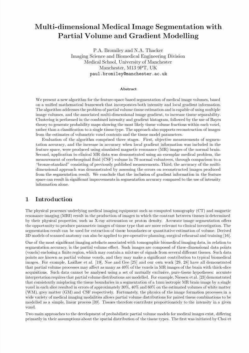
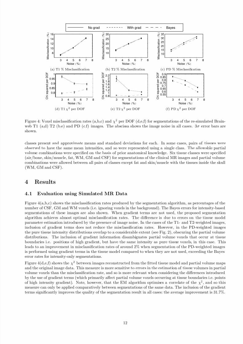
Figure 4: Voxel misclassification rates (a,b,c) and χ2 per DOF (d,e,f) for segmentations of the re-simulated Brain-web T1 (a,d) T2 (b,e) and PD (c,f) images. The abscissa shows the image noise in all cases. 3σ error bars areshown.

classes present and approximate means and standard deviations for each. In some cases, pairs of tissues wereobserved to have the same mean intensities, and so were represented using a single class. The allowable partialvolume combinations were specified on the basis of prior anatomical knowledge. Six tissue classes were specified(air/bone, skin/muscle, fat, WM, GM and CSF) for segmentations of the clinical MR images and partial volumecombinations were allowed between all pairs of classes except fat and skin/muscle with the tissues inside the skull(WM, GM and CSF).

4 Results

4.1 Evaluation using Simulated MR Data

Figure 4(a,b,c) shows the misclassification rates produced by the segmentation algorithm, as percentages of thenumber of CSF, GM and WM voxels (i.e. ignoring voxels in the background). The Bayes errors for intensity-basedsegmentations of these images are also shown. When gradient terms are not used, the proposed segmentationalgorithm achieves almost optimal misclassification rates. The difference is due to errors on the tissue modelparameter estimation introduced by the presence of image noise. In the cases of the T1- and T2-weighted images,inclusion of gradient terms does not reduce the misclassification rates. However, in the PD-weighted imagesthe pure tissue intensity distributions overlap to a considerable extent (see Fig. 2), obscuring the partial volumedistributions. The inclusion of gradient information disambiguates partial volume voxels that occur at tissue

boundaries i.e. positions of high gradient, but have the same intensity as pure tissue voxels, in this case. Thisleads to an improvement in misclassification rates of around 2% when segmentation of the PD-weighted imagesis performed using gradient terms in the tissue model compared to when they are not used, exceeding the Bayeserror rates for intensity-only segmentations.

Figure 4(d,e,f) shows the χ2 between images reconstructed from the fitted tissue model and partial volume mapsand the original image data. This measure is more sensitive to errors in the estimation of tissue volumes in partialvolume voxels than the misclassification rate, and so is more relevant when considering the differences introducedby the use of gradient terms (which primarily affect partial volume voxels occurring at tissue boundaries i.e. pointsof high intensity gradient). Note, however, that the EM algorithm optimises a correlate of the χ2, and so thismeasure can only be applied comparatively between segmentations of the same data. The inclusion of the gradientterms significantly improves the quality of the segmentation result in all cases: the average improvement is 31.7%.

12



(a) (b) (c) (d)

Figure 6: Reconstructed MR data: IRTSE(a), VE (PD) (b) VE (T2) (c) and FLAIR (d)

FLAIR

0.2 0.3 0.4 0.5 0.6

Monte-Carlo Stability

1000

2000

3000

4000

5000

R e s i d u a l O u t l i e r M e a s u r e Median Filtering

Gaussian Smoothing

Tangential Smoothing

NL MeansMulti-spectral

Figure 7: Residual outlier measure vs. Monte-Carlo stability.

improving noise removal characteristics, whilst Gaussian filtering removes significantly more noise at the expenseof degrading the images significantly. Excluding the FLAIR image result, the multispectral image reconstruction ison average approximately twice as destructive as tangential smoothing: the intensity model fits the data well for allbut around 6% of the voxels in the images. The ROM for the FLAIR image is higher as such images are susceptibleto flow artefacts. The cerebral vasculature, and some voxels in the CSF compartments, therefore form extra tissueclasses not included in the tissue model, leading to misinterpretation of such voxels. The non-local means algorithmrepresents a state-of-the-art noise filter, and removes approximately half of the noise whilst achieving an averageROM of ≈ 100, about 50% higher than the theoretical optimum. This is due to the incorporation of an explicit testof similarity; during the averaging process the voxels are weighted by their similarity to the voxel being filtered.The algorithm therefore avoids averaging over voxels drawn, for example, from different sides of a tissue boundary,and so preserves image structure. However, when the similarity test is applied to voxels with high levels of noisei.e. those in the tails of the intensity distributions, few voxels with similar intensities will be found. Such voxels willtherefore be left largely unmodified due to a lack of data to incorporate into the averaging process. Non-local meanstherefore achieves a low ROM by definition, at the expense of applying a spatially varying amount of smoothingand producing an output with spatially varying noise.

5 Discussion and Conclusions

In previous work we have extended standard volumetric estimation techniques to multiple images. In this worka method to utilise not only the intensity information but also the local intensity gradient information in a MRimage was described. The method can be considered as an alternative both to the assumption of local regionalsmoothness and to local resampling of the prior probabilities, which have previously been suggested by otherauthors [19]. Unlike these methods, local structural information is used directly in a manner that is quantitativelyrelated to the image formation process.

14



Several evaluation methodologies were applied to the algorithm. In unispectral segmentation of simulated datausing intensity information alone, the algorithm achieved almost optimal tissue classification. The addition of gradient information resulted in significant improvements in images where the pure tissue intensity distributionsoverlap to a significant extent, due to the ability of gradient information to disambiguate pure tissue and partialvolume classes with similar intensities. The χ2 measure indicated significant improvements in partial volumeestimation in all cases when gradient information was included. Evaluation of unispectral segmentation on clinicalimages indicated that the algorithm showed no significant systematic error in the CSF volume measurement task,

and achieved lower random errors than alternative techniques. It should be noted that this study did not evaluatethe performance on repeated acquisitions from the same subject, since a lower random error limit is imposed by theintrinsic biological variability in CSF measurements, but it does indicate the expected performance of the algorithmin transverse volume measurement studies. The proposed algorithm is therefore capable of providing increasedstatistical power with which to detect volume changes or differentiate between subject groups in such studies. Inaddition, the comparison indicated that the SPM software, a de-facto standard in medical image analysis, producedsignificantly higher estimates of CSF volume than are supported by the consensus of the literature.

Evaluation of the multi-spectral application of the algorithm focused on measuring the goodness-of-fit of the tissuemodel, and indicated that the model fits the data well for all but approximately 6% of the voxels. In addition, thisevaluation methodology demonstrates the use of the multispectral segmentation as a noise-filtering technique. Ingeneral multi-spectral filtering was shown to be no more destructive to image contents than median filtering butremoved more image noise than Gaussian smoothing. Therefore, such reconstruction techniques may be a useful

way of processing multiple MR acquisitions.The main limitation of the algorithm presented here is the assumption, in common with previous authors (e.g.[31, 19]) of a uniform distribution for partial volume voxels. As described above, other authors have investigatednon-uniform distributions with some success, and Chiverton [8] has investigated the incorporation of non-uniformpartial volume distributions into the formulation described here. In addition, the EM update scheme used hereassumes spatial independence in the noise. Finally, the region to be segmented must contain a sufficient quantityof pure tissues to allow model fitting; it may therefore not be applicable to segmentations limited to regions suchas the basal ganglia, which consist primarily of partial volume voxels at the resolution of MR images.

6 Acknowledgements

We acknowledge the contributions of Prof. A. Jackson, Dr. M. Pokric, Dr. M. Scott and Dr. D. Williamson tothe early stages of this work, and the the help of Profs. P. Rabbitt and C. Hutchinson with MR data collection.Part of this work was conducted during the course of a special MRC training fellowship and support was alsoreceived under the EPSRC/MRC funded MIAS IRC (from Medical Images and Signals to Clinical InformationInterdisciplinary Research Collaboration), under EPSRC GR/N14248/01, and UK MRC Grant No. D2025/31.The software and associated technical notes are available at www.tina-vision.net.

References

[1] D D Blatter, E D Bigler, S D Gale, S C Johnson, C V Anderson, B M Burnett, N Parker, S Kurth, and S DHorn. Quantitative volumetric analysis of brain MR: Normative database spanning 5 decades of life. AJNR

Am J Neuroradiol , 16:241–251, 1995.

[2] P A Bromiley. TINA Memo No. 2008-009: The TINA medical image segmentation algorithm: Mathematicalderivations and proofs. Technical report, Imaging Sceince and Biomedical Engineering, School of Cancer andImaging Sciences, University of Manchester, 2008. http://www.tina-vision.net/docs/memos/2008-009.pdf.

[3] P A Bromiley, N A Thacker, and P Courtney. Non-parametric image subtraction using grey level scattergrams.Image and Vision Computing , 20:609–617, 2002.

[4] P A Bromiley, N A Thacker, and A Jackson. Trends in brain volume change with normal ageing. In Proc.MIUA’05 , pages 247–250, 2005.

[5] P A Bromiley, N A Thacker, M L J Scott, M Pokric, A J Lacey, and T F Cootes. Bayesian and non-Bayesianprobabilistic models for medical image analysis. Image and Vision Computing , 21(10):851–864, 2003.

[6] D Chan, N C Fox, R I Scahill, W R Crum, J L Whitwell, G Leschziner, A M Rossor, J M Stevens, L Cipolotti,and M N Rossor. Patterns of temporal lobe atrophy in Alzheimer’s disease. Ann Neurol , 49:433–442, 2001.

15



[7] D T Chard, G J M Parker, C M B Griffin, A J Thompson, and D H Miller. The reproducibility and sensitivityof brain tissue volume measurements derived from an SPM-based segmentation methodology. J Magn Reson Imaging , 15:259–267, 2002.

[8] J P Chiverton. Probabilistic Partial Volume Modelling of Biomedical Tomographic Image Data . PhD thesis,Center for Vision, Speech and Signal Processing, University of Surrey, Guildford, Surrey GU2 7HX, U.K.,Aug 2006.

[9] H S Choi, D R Haynor, and Y Kim. Partial volume tissue classification of multichannel magnetic resonanceimages-a mixture model. IEEE Trans Med Imaging , 10:395–407, 1991.

[10] C E Coffey, J A Saxton, G Ratcliff, R N Bryan, and J F Lucke. Relation of education to brain size in normalaging: Implications for the reserve hypothesis. Neurology , 53:189–196, 1999.

[11] A P Dempster, N M Laird, and D B Rubin. Maximum likelihood from incomplete data via the EM algorithm.Journal of the Royal Society , 39:1–38, 1977.

[12] K Fukenaga. Introduction to Statistical Pattern Recognition . Academic Press, San Diego, 2nd edition, 1990.

[13] C D Good, I S Johnsrude, J Ashburner, R N A Henson, K J Friston, and R S J Frackowiak. A voxel-basedmorphometric study of ageing in 465 normal adult human brains. NeuroImage , 14:21–36, 2001.

[14] H Gudjbartson and S Patz. The Rician distribution of noisy MRI data. Magn Reson Med , 34(6):910–914,1995.

[15] R C Gur, P D Mozley, S M Resnick, G L Gottlieb, M Kohn, R Zimmerman, G Herman, S Atlas, R Grossman,D Berretta, R Erwin, and R E Gur. Gender differences in age effect on brain atrophy measured by magneticresonance imaging. Proc Natl Acad Sci USA, 88:2845–2849, 1991.

[16] N W John, N A Thacker, M Pokric, and A Jackson. An integrated simulator for surgery of the petrous bone.In Medicine Meets Virtual Reality 2001, pages 218–224. IOS Press, 2001.

[17] N Joshi and J M Brady. A non-parametric model for partial volume segmentation of MR images. In Proceedings BMVC’05 , pages 919–928, 2005.

[18] R K-S Kwan, A C Evans, and G B Pike. MRI simulation-based evaluation of image-processing and classification

methods. IEEE Trans Med Imaging , 18(11):1085–1097, 1999.

[19] D H Laidlaw, K W Fleischer, and A H Barr. Partial-volume Bayesian classification of material mixtures inMR volume data using voxel histograms. IEEE Trans Med Imaging , 17(1):74–86, 1998.

[20] K Van Leemput, F Mayes, D Vandermuelen, and P Suetens. A unifying framework for partial volume seg-mentation of brain MR images. IEEE Trans Med Imaging , 22(1):105–119, 2003.

[21] J V Manjon, M Robles, and N Thacker. Multispectral MRI de-noising using non-local means. In Proc.MIUA’07 , pages 41–45, Aberystwyth, Wales, 2007.

[22] E Mueller, M M Moore, D C R Kerr, G Sexton, R M Camicioli, D B Howieson, J F Quinn, and J A Kaye.Brain volume preserved in healthy elderly through the eleventh decade. Neurology , 51:1555–1562, 1998.

[23] W J Niessen, K L Vincken, J Weickert, B M Ter Haar Romeny, and M A Viergever. Multiscale segmentationof three-dimensional MR brain images. International Journal of Computer Vision , 31:185–202, 1999.

[24] L Nocera and G C Gee. Robust partial volume tissue classification of cerebral MR scans. In K M Hanson,editor, Proc. SPIE Medical Imaging 1997: Volume 3034 of SPIE Proceedings , pages 312–322, 1997.

[25] A Noe and J C Gee. Partial volume segmentation of cerebral MRI scans with mixture model clustering. InProc. IPMI’01, pages 423–430, 2001.

[26] S I Olsen. Estimation of noise in images: An evaluation. CVGIP: Graphical Models and Image Processing ,55:319–323, 1993.

[27] D L Pham and J L Prince. Unsupervised partial volume estimation in single-channel image data. In Proc.IEEE Workshop Mathematical Methods in Biomedical Image Analysis-MMBIA’00 , pages 170–177, 2000.

[28] M Pokric, N A Thacker, and A Jackson. The importance of partial voluming in multi-dimensional medicalimage segmentation. In Proc. MICCAI’01, pages 1293–1294, 2001.

16



[29] M Pokric, N A Thacker, M L J Scott, and A Jackson. Multi-dimensional medical image segmentation withpartial voluming. In Proc. MIUA’01, pages 77–80, 2001.

[30] S Ruan, C Jaggi, J Xue, J Fadili, and D Bloyet. Brain tissue classification of magnetic resonance images usingpartial volume modelling. IEEE Trans Med Imaging , 19:1179–1187, 2000.

[31] P Santago and H D Gage. Quantification of MR brain images by mixture density and partial volume modelling.IEEE Trans Med Imaging , 12:566–574, 1993.

[32] P Santago and H D Gage. Statistical models of partial volume effect. IEEE Trans Image Processing , 4:1531–1540, 1995.

[33] D W Shattuck, S R Sandor-Leahy, K A Schaper, D A Rottenberg, and R M Leahy. Magnetic resonance imagetissue classification using a partial volume model. NeuroImage , 13:856–876, 2001.

[34] N A Thacker, A Jackson, and D Moriarty. Improved quality of re-sliced MR images using renormalised sincinterpolation. J Magn Reson Imaging , 10:582–588, 1999.

[35] N A. Thacker, A J Lacey, and P A Bromiley. Validating MRI field homogeneity correction using imageinformation measures. In Proc. BMVC’02 , pages 626–635, 2002.

[36] N A Thacker, M Pokric, and D C Williamson. Noise filtering and testing illustrated using a multi-dimensional

partial volume model of MR data. In Proc. BMVC , pages 909–919, Kingston, London, 2004.

[37] N A Thacker, D C Williamson, and M Pokric. Multi-dimensional MR image segmentation with gradientanalysis. In Proc. MIUA’05 , pages 23–26, Bristol, 19th-20th July, 2005.

[38] J Tohka, E Krestyannikov, I D Dinov, A MacKenzie Graham, D W Shattuk, U Ruotsalainen, and A W Toga.Genetic algorithms for finite mixture model based voxel classification in neuroimaging. IEEE Trans. Med.Imag., 26:696–711, 2007.

[39] S Webb. The Physics of Medical Imaging . Medical Science Series. Adam Hilge, Bristol, Philadelphia and NewYork, 1988.

[40] J L Whitwell, W R Crum, H C Watt, and N C Fox. Normalisation of cerebral volumes by use of intracranialvolume: Implications for longitudinal quantitative MR imaging. Am J Neuroradiol , 22:1483–1489, 2001.

[41] D C Williamson, N A Thacker, S R Williams, and M Pokric. Partial volume tissue segmentation usinggrey-level gradient. In Proc. MIUA’02 , pages 17–20, 2002.

17

multi-dimensional medical image segmentation with partial volume and gradient modelling

Documents