Multi-degree-of-freedom robot arm motion simulation based on MATLAB

Bin Guo1,a,* 1School of Electrical and Computer Engineering, Nanfang College of Sun Yat-sen University,

Guangdong, 202104, China a.binguo19990927@gmail.com

*corresponding author

Keywords: The Multi-degree-of-freedom robotic arm, Kinematic analysis, Work space and trajectory planning, MATLAB

Abstract: The design is divided into three main parts. The first part is an analysis of the basis robotic arm components and principles to understand how the robotic arm is precisely and automatically controlled to achieve the desired task. The kinematic basis of the robotic arm is then investigated by establishing a co-ordinate system for the arm based on the modified D-H method. A preliminary kinematic model of the 6 degree of freedom robotic arm is established through a structural study of ABB's multi-degree-of-freedom robot. The basic parameters of the robotic arm are brought into the equation to obtain its equations of motion, and then a simulation study is carried out using MATLB to find the forward and inverse solutions, and the results are compared with the previous study to verify their reasonableness. The second part is based on the description and analysis of the work space in the first part, and the methods for solving the work space are investigated. These methods are also compared to analyse and understand their applicability and reasonableness. Finally, the path description and generation of the robotic arm is studied to complete the planning of the robotic arm trajectory and the results of the simulation are analysed. The study of the 6-degree-of-freedom robot arm is used to improve the theoretical basis of the robot. The study of the 6-degree-of-freedom robotic arm provides a deeper understanding of the structural parameters of the robot arm and adds to the missing knowledge for the next study of intelligent robotics, as well as to the research and application of the robotic arm or to further research based on it.

1. Introduction

With the continuous improvement and development of computer technology, the use of robotics in people's lives has become common. Many countries are also paying more attention to robotics research, and have made it a strategic national priority to support and develop it. As a prototype of industrial robotics, the multi-degree-of-freedom robot arm is widely used in various fields because it can imitate the movements of a human arm to perform dangerous, complex and single tasks.

Journal of Engineering Mechanics and Machinery (2021) Vol. 6: 42-69 Clausius Scientific Press, Canada

DOI: 10.23977/jemm.2021.060107 ISSN 2371-9133

42

1.1. Background and significance of the subject

With the continuous development of mechanisation and intelligence, the field of industrial robotics is becoming more and more widely used up and crossed with several fields. The work of robots is largely dependent on the movement of robotic arms, so it is said that multi-degree-of-freedom robotic arms are the prototype of industrial robots. As a result of the rapid technological and economic development brings a series of needs, companies seek higher production efficiency and quality, and people seek a higher level of quality of life. In this environment, a variety of robots such as rescue and search, home service and industrial production are slowly emerging. Robotic arms, as an important part of robotics, have been one of the main focuses of robotics research. In particular, the robotics industry has been in a phase of rapid development, and as a result, people are slowly being replaced by robots that can help free them from heavy, repetitive, monotonous work and other high-risk tasks. The robotics industry is also known as the 'jewel in the manufacturing crown', which shows how important the use of industrial robots is to the manufacturing industry. It is therefore particularly important to see how innovative the manufacturing of robotic arms is, which requires us to keep moving forward on the road of independent innovation.

The robotic arm can move freely within a certain space, completing a series of complex movements that are difficult to match artificially to achieve a set goal, mainly consisting of a number of different jointed arm claws, bases, etc., most of which have many joints. For radioactive materials that cannot be handled manually, the Argonne National Energy Laboratory in the USA first developed a remote-controlled robotic arm to handle nuclear contaminated materials as early as after the Second World War to solve the problem of radioactive material handling. This has, to some extent, solved the problem of exposing experimenters to radioactive substances for long periods of time to the extent that their health was greatly affected. It was in this context that the multi-degree-of-freedom robotic arm first appeared in a real-world application. In 1959, the first prototype industrial robot, the Unimate, was invented and built by the American inventors George Devol and Joseph F·Engelberger, and this led to the establishment of Unimation, the world's first industrial robot manufacturing facility[1]. The explosive development of computer technology in the 1980s led to the expansion of the field of application of robotic arms, the limitations of their use were gradually reduced and the study of control algorithms for robotic arms became increasingly important. The latest trend in modern manufacturing automation is the application of robotic arms in combination with computer design systems and auxiliary manufacturing systems in many ways.

The latest survey by IFR reports that more than 2.7 million industrial robots are already in operation in factories in China, Japan, the US, Germany and several other countries in order to open up the demand for automation retrofits, expand the market and increase the number of industrial robots put into operation worldwide. Over a five-year period, the number of robots installed nationwide in 2019 has increased by almost 85% compared to 2014. But the global economy has received an unassessable blow as a result of the new crown epidemic, and sales have already declined marginally. The exception may be China, where the economy is in a phase of rapid recovery at a time when other countries are in a turnaround phase. It is clear from this that China's industrial robots are developing at a sustained and very rapid rate, and from the low level of competition that has emerged in the industry, the prospects for China's domestic industrial robots have always been good, and the market is becoming increasingly competitive. Essential to the future of manufacturing equipment is robotics, which has a prominent role in the future development of the country. The Made in China 2025 clearly states that the development of intelligent equipment, especially robotics, should be the focus of development. As all major countries around the world are vigorously developing manufacturing technology and making robotics research a key development, it is said that China is gradually recognising its importance.

43

Subjectively speaking, the development of robotics will largely determine the future of the world. With strong robotics technology, we can have cheap labour costs and better control of sophisticated core technologies, and countries are constantly increasing their investment in robotics to be at the forefront of the world. In the foreseeable future, the era of robots replacing manual labour will soon come with an increase in the number of robots.

There are two mainstream approaches to the study of control algorithms for multiple degrees of freedom robotic arms: the indirect approach and the direct approach. The indirect method is to perform offline simulation studies on an interface programming application such as Matlab or VC, and then apply the simulation algorithms and results to a physical robotic arm controller for testing and verification; the direct method is to design and debug the algorithms directly on the robotic arm in real time[2], mainly based on hardware-in-the-loop real-time simulation systems (e.g. Dspace, RT-LAB, etc.) .

To reproduce the motion of the arm using the function set by means of Matlab simulation, a mathematical model of the multi-degree-of-freedom arm needs to be built so that we can visually monitor the motion of the various parts of the arm. Secondly, the control algorithm is designed using the toolbox provided by Simulink, and then the algorithm is verified and some modifications and optimisations are made, which is an advantage. The disadvantage of this is that it is somewhat detached from the actual robot arm and there are many factors that can affect its movement in reality. So it is very difficult to create a mathematical model that fits perfectly with the actual situation. The simulation results alone are not enough, and most of them need to be re-tuned and modified on the real object, which results in a waste of time and resources. This can be solved by a real-time simulation, where the computer is directly connected to the hardware and the host computer sends commands to the hardware system, which then executes the commands and returns the experimental data to the host computer, and finally the computer processes and analyses the experimental results.

This topic does not investigate the real-time simulation system in detail, but mainly uses the D-H method parameters to model the robot arm. This time, while analysing the applicability of the control algorithm, the mechanism of the robot at work, the space, and the validity of the solution of the robot kinematic and inverse kinematic equations are investigated. Robotics toolbox helps us to solve relevant simulations about robotics, based on the kinematic problems and spatial planning law problems of the robotic arm and joints, for the control strategy of the robotic arm It provides a theoretical basis.

1.2. Research status of multi-degree-of-freedom robotic arms at home and abroad

1.2.1. Current status of foreign research on multi-degree-of-freedom robotic arms

Foreign research on robotic arms first began in the 1940s and its development history has been more than 80 years since then. In recent years domestic and foreign research on multi-degree-of-freedom robotic arms has centred on kinematic analysis, work space analysis, optimised design and trajectory planning control methods for robotic arms. The basic theory of research on robotic arms has been a small achievement thanks to the efforts of scholars in various countries at home and abroad, but foreign research is still at the forefront compared to domestic research.

Robotics-related technological devices have been developing rapidly since Joseph F·Engelberger and George Devol in the USA worked together to create the first-ever programmable algorithm-appropriate robots for industry. The importance of robotics has become equal to that of the Internet in the US national development plan, and countries such as the US have made meticulous plans for the development of robotics. At the same time, the European Union has not been shy about initiating significant funding to promote the development of robotics, and Japan, a relatively mature

44

country in robotics, also sees it as a key development target. Some developed countries, such as the US and Japan, have themselves taken great advantage of research into robotics, and they are putting robotics into different areas instead of manual labour to make robotics even more rapidly developed. The field of application of robotics will continue to widen, with high-technology industries, such as aviation, also using robotics. The use of robotics in high-technology fields requires robotic arms to move towards high precision, intelligence, modularity, biomimetics, miniaturisation, energy efficiency and environmental protection. From the most common industrial robotic arms all the way to space robotic arms, medical robotic arms and a range of other complex robotic arms, foreign countries are in the lead. The non-invasive idea-controlled robotic arm technology was developed by Professor Bin He of Carnegie Mellon University and his research team in collaboration with the University of Minnesota, using brain-computer technology to connect with the brain non-invasively[3], without the need for surgical implantation of a chip to obtain nerve signals through the human scalp to manipulate the robotic arm. It can control the arm based on fantasies in the human brain, tracking a cursor that moves at any time.

Figure 1: Schematic diagram of a non-invasive mind-controlled robotic arm frame.

In terms of the development of foreign robots, the technology of robotic arms for industrial use has become very mature, both in terms of design and control, and their current standards are recognised and have become the standard for the industry. The world's major robotic arm manufacturers are also dominated by foreign companies, including Fanuc, Yaskawa and Yamaha in Japan, KUKA in Germany and ABB in Switzerland. From the parameters and functions of the robotic arms introduced for industrial use, it can be inferred that the technology is being developed along the path of artificial intelligence control and miniaturisation of the system. And through a series of optimisation such as re-optimisation of the actual working environment and flexibility of the task, the robot arm can achieve high performance functions such as high speed, high precision and high reliability, thus achieving cost reduction and efficiency improvement.

45

Figure 2: Industrial robotic arm products of foreign companies.

1.2.2. Current status of domestic research on multi-degree-of-freedom robotic arms

Although China's emphasis on robotics has gradually increased, it is undeniable that the gap between us and developed countries is still relatively obvious. In China, research into industrial robotic arms began in the 1980s, and by the early 1990s the first batch of special robotic arms had been successfully developed. In 1987-1993, drawing on the research history of foreign robotic arms, the country planned its own robotic arm technology development goals, expecting to achieve all-round robotic arm coverage in the industrial field in 2000, while the country's efforts to develop special robotic arm applications in outer space exploration, medical operations and deep-sea exploration and other fields to reduce the risk of human work. During that period, the Seventh Five-Year Plan was mainly devoted to robotics, and the vision of robotics was incorporated into the 863 programme. The bipedal walking robot developed by the Harbin Institute of Technology was a testament to the times[2].

The design and optimisation of industrial robotic arms, the hardware design of control and drive systems, the design of software systems for robotic arms, kinematics and trajectory planning have now been mastered by some military companies, research institutes and enterprises, and have even reached the world's advanced level in key technologies. Unfortunately, patents related to the field of robotic arms have been applied for in large numbers by foreign companies in China. Because some technologies are less mature due to the short development time of domestic robotics, the number of patents owned by the control unit design and motor technology of robotic arms is low, so domestic enterprises are forced to import relevant parts to produce industrial robotic arms[4]. This has led to high costs for domestic enterprises to produce robotic arms, and also to be hamstrung by foreign companies thus leaving us without upper-level competitiveness.

This is why there is a need to continuously improve the technology in order to achieve outstanding results in robotics. Firstly, an optimised robot arm structure is needed to make it more flexible, a good hardware working base is also indispensable, and the rationalisation of the movement must be ensured. Secondly, errors in the control of repeated robotic arms are reduced and automatically corrected so that they remain highly accurate when repeating a single task. Finally, optimising the trajectory and structure of the robot arm, based on existing technology in robot arm design, needs to be improved according to the different design requirements. The above-mentioned is the basis for the flourishing development of robotics, which is crucial to the development of research and application of robotics.

To date, domestic robotics of an industrial nature has steadily developed, with an increasing variety of different industrial robots being put into use and leading global industrial robot giants looking favourably on our country. Despite the growing competition in robotics at home and abroad, the gap between Chinese and foreign companies will become smaller and the technology

46

will become more mature by world layout. For example, the industrial robots produced by SIASUN Robotics, a new company invested by the Chinese Academy of Sciences Shenyang Institute of Automation, and the GSK series of industrial robotic arms from Guangzhou NC, are proof of the rapid development of industrial robotic arm technology in China.

Figure 3: Industrial robotic arm products of domestic companies.

1.3. Main research content of the thesis

Based on the structure and parameters of the six-degree-of-freedom robotic arm at home and abroad, kinematic analysis and work space analysis will be carried out on it. The STM32F103 chip is used for the upper control of the STM32 micro controller, which mainly controls the positioning of the robot arm and the movement of the arm through algorithms. The algorithm analysis of the STM32 micro controller is required to achieve effective control of the PWM waves and to provide stable control of the robot arm to achieve multi-degree of freedom rotation. The mathematical model and trajectory planning of the robot arm are simulated using Matlab software, and the rationality of the arm is analysed. Details are described as follows.

Chapter 1: To understand and analyse the background and significance of the research of the topic, as well as to collect information about the development status and latest product applications at home and abroad and compare them.

Chapter 2: The STM32F103 chip microprocessor is used for the upper control system to analyse and design the composition and principle of the robotic arm, through the study to understand how the robotic arm can be accurately and automatically controlled to achieve efficient and stable work.

Chapter 3: Analyse the kinematic aspects of the robot arm and construct a mathematical model, consider the multi-degree-of-freedom robot arm as a control object and build a motion model based on D-H, deduce and generalise the forward and inverse solutions of the robot arm, simulate the results and debug the parameters through Matlab applications.

Chapter 4: Analyse the applicability of trajectory planning in the work space, compare the methods of trajectory planning, analyse the experimental results and draw conclusions based on the issues and performance indicators that should be paid attention to when trajectory planning.

Chapter 5: Matlab simulation analysis of the six-degree-of-freedom robotic arm in conjunction with the above research, and an overall summary.

47

2. Composition and principle of multi-degree-of-freedom robotic arms

2.1. Drive modules

The signal control of the robot arm requires the reception of the machine's channels and then signal modulation of the chip in order to achieve an accurate and timely acquisition of the DC bias voltage. In order for the voltage difference to be output effectively, the obtained DC bias voltage is compared with the voltage difference of the potentiometer and the reference circuit is included in the drive module of the robot arm. The potentiometer is driven by a coupled reduction gear to rotate as the motor speed is maintained. The position detector infers the accuracy of the positioning based on the signals sent back. The motor stops rotating when the voltage difference is zero. As the driver for the position servo, the servo ensures that the control system is maintained even when the angle is constantly changing.

2.2. Gyroscope modules

In the direction of the axis of rotation, a rotating object is unaffected by external forces, which is the mechanism of a gyroscope. A gyroscope relies on rotation to keep itself in balance; a gyroscope at rest would have its balance destroyed by external forces. A gyroscope in a rotating state can reach hundreds of thousands of revolutions per minute, so that it can work for long periods of time and be stable. The gyroscope module uses currently known methods to read the gyroscope direction and then automatically transmits these data signals to the control system.

The MPU6050 is an integrated six-axis motion processing assembly with a three-axis gyroscope that detects the rotation speed of the corresponding axis, and a three-axis accelerometer that ranges the analogue signal and converts the acceleration to a digital readout via an internal ADC. And there is an on-chip 1024 byte FIFO that reduces the power consumption of the OS for motion processing operations. Its communication with all device registers is mediated by the main I2C interface, which allows the complete 9-axis attitude fusion algorithm data to be output to the application segment for easy attitude resolution.

2.3. Control modules

The STM32F103 micro controller uses the Cortex-M3 core with a maximum CPU speed of 72 MHz. Its family portfolio covers from 16K bytes to 1 MB of Flash and is equipped with motor control peripherals, USB full speed interface and CAN for better control of robotic arms.

2.4. Implementation modules

In the control of robotic arm actuation modules, the arm structure is usually selected scientifically and rationally by the working environment in order to allow the arm to do its job better, and it just so happens that the end-effector structure can be varied. These include gripping jaws and air-flow suction cups, which can be used for different needs to complete commands more efficiently.

48

Figure 4: End-effector structure of the robot arm.

2.5. Implementation modules

In summary, the robotic arm uses the STM32F103 series micro controller as the control core and is able to carry out the basic behavioural actions of the robotic arm normally. At the same time the digital six-axis gyroscope sensor is used as a common part with the robot arm at the same time, enabling the timely and accurate collection of spatial information and other data at a set frequency. The spatial position information is then accurately transmitted to the STM32 host control system via the SPI communication protocol. Positioning algorithm control and motion control these two methods are the main way to control the basic action of the robot arm, to have an accurate control of the PWM wave need to control the servo of the robot arm need the STM32 information processing, through this way can be faster positioning to the need to operate the control position, to achieve automation and accuracy of the robot arm control.

3. Kinematic analysis of multi-degree-of-freedom robotic arms

3.1. Introduction

Kinematics is simply the neglect of the forces that cause this motion and under these conditions the analysis of the object's motion and the relationship between the amounts of motion. In this case the kinematic analysis of a robotic arm is the analysis of the full geometrical and temporal characteristics of the motion. The end-effector is usually installed at the end of the robot arm, and the tool coordinate system on the end-effector will be used to explain the position of the operating arm in relation to the base coordinate system set on the base of the arm's operating base, and in this way the kinematics of the robot arm is divided into two types. One is positive kinematics, which is really a static geometry problem to calculate the position and attitude of the arm's end-effector, while the other is inverse kinematics, where the position and attitude of the end-effector are given and then the joint angle is calculated to meet the desired requirements. More precisely, this extends to the study of position, velocity, acceleration and the higher order differentiation of position variables with respect to time or other variables. It can be said that kinematic analysis is a prerequisite and a basis for mechanism analysis and is of great importance to the research work on robotic arms.

49

Figure 5: Positive kinematic analysis.

Figure 6: Inverse kinematic analysis.

Nowadays, the development of computer technology has been so perfect that the solution of inverse kinematics for robotic arms has gradually changed from the traditional geometric, iterative and analytical methods to some intelligent optimisation algorithms including Particle swarm algorithm, Genetic algorithm, Neural network algorithm, etc. algorithm, etc. With the tremendous increase in computer speed and carrying capacity, the optimisation of the performance of intelligent algorithms for inverse kinematic solutions has become one of the most important research directions for robotic arms today. A very practical method for solving kinematics is currently being used in research on related topics. It was jointly proposed by Denavit and Hartenberg and is mainly used to establish the linkage coordinate system and is called the D-H method. Due to the practical nature of the method, it has been used extensively in the study of robotic arm kinematics. After the robot model is established using the D-H method, the kinematic equations are first obtained by analysing the linkage and movable joints of the robot arm. To know the transformation matrix of all

50

movable joints, a reference coordinate system must first be defined for each movable joint of the robot and then, starting from the base and for each joint, the total transformation matrix of the movable joints is determined. Based on the matrix representing the transformation of the movement and direction of the joints, the kinematic equations of the tandem robot arm are finally determined.

3.2. Fundamentals of robot kinematics

3.2.1. Displacement of robot kinematics

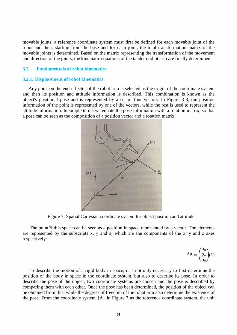
Any point on the end-effector of the robot arm is selected as the origin of the coordinate system and then its position and attitude information is described. This combination is known as the object's positional pose and is represented by a set of four vectors. In Figure 3-3, the position information of the point is represented by one of the vectors, while the rest is used to represent the attitude information. In simple terms we equate the pose information with a rotation matrix, so that a pose can be seen as the composition of a position vector and a rotation matrix.

Figure 7: Spatial Cartesian coordinate system for object position and attitude.

The point P A this space can be seen as a position in space represented by a vector. The elements are represented by the subscripts x, y and z, which are the components of the x, y and z axes respectively:

P A = �pxpypz�(1)

To describe the motion of a rigid body in space, it is not only necessary to first determine the

position of the body in space in the coordinate system, but also to describe its pose. In order to describe the pose of the object, two coordinate systems are chosen and the pose is described by comparing them with each other. Once the pose has been determined, the position of the object can be obtained from this, while the degrees of freedom of the robot arm also determine the existence of the pose. From the coordinate system {A} in Figure 7 as the reference coordinate system, the unit

51

vectors of its principal axes in the fixed coordinate system {B} are set to be 𝑋𝑋 𝐵𝐵 、 𝑌𝑌 𝐵𝐵 、 𝑍𝑍 𝐵𝐵 . The results can be expressed as 𝑋𝑋 𝐴𝐴 𝐵𝐵 、 𝑌𝑌 𝐴𝐴 𝐵𝐵 and 𝑍𝑍 𝐴𝐴 𝐵𝐵 . If they are arranged in order to form a 3*3 matrix (the {B} rotation matrix with respect to {A}), denoted by the symbol 𝑅𝑅𝐵𝐵𝐴𝐴 :

𝑅𝑅 = ( 𝑋𝑋 𝐴𝐴 𝐵𝐵 𝑌𝑌 𝐴𝐴 𝐵𝐵 𝑍𝑍 𝐴𝐴 𝐵𝐵 ) = �𝑟𝑟11 𝑟𝑟12 𝑟𝑟13𝑟𝑟21 𝑟𝑟22 𝑟𝑟23𝑟𝑟31 𝑟𝑟32 𝑟𝑟33

�𝐵𝐵𝐴𝐴 (2)

Accordingly, the equivalent angle-axis representation can be used to find the equivalent rotation

matrix around one of the major axes as the axis of rotation, expressed respectively as:

𝑅𝑅𝑋𝑋(𝜃𝜃) = �1 0 00 𝑐𝑐𝑐𝑐𝑐𝑐𝜃𝜃 −𝑐𝑐𝑠𝑠𝑠𝑠𝜃𝜃0 𝑐𝑐𝑠𝑠𝑠𝑠𝜃𝜃 𝑐𝑐𝑐𝑐𝑐𝑐𝜃𝜃

�(3)

𝑅𝑅𝑌𝑌(𝜃𝜃) = �𝑐𝑐𝑐𝑐𝑐𝑐𝜃𝜃 0 𝑐𝑐𝑠𝑠𝑠𝑠𝜃𝜃

0 1 0−𝑐𝑐𝑠𝑠𝑠𝑠𝜃𝜃 0 𝑐𝑐𝑐𝑐𝑐𝑐𝜃𝜃

�(4)

𝑅𝑅𝑍𝑍(𝜃𝜃) = �𝑐𝑐𝑐𝑐𝑐𝑐𝜃𝜃 −𝑐𝑐𝑠𝑠𝑠𝑠𝜃𝜃 0𝑐𝑐𝑠𝑠𝑠𝑠𝜃𝜃 𝑐𝑐𝑐𝑐𝑐𝑐𝜃𝜃 0

0 0 1� (5)

The coordinates of the actuators at the end of the robot arm will change as the coordinates of

each joint change. Only by dealing with the changes in the coordinates of each joint and establishing the relationship between the base and end coordinates can the condition of the end coordinates be accurately determined. There are two main types of coordinate transformation used, one called translation transformation and the other called rotation transformation.

Figure 8: Coordinate system by translation and rotation.

A translation transformation is simply a point moving in a known vector direction, and a translation of a spatial point is a mapping of one more spatial coordinate system to another based on this, which is numerically described in the same way. Suppose that vector is P 1

A translated through vector Q A ,resulting in a new vector P 2

A , calculated as follows:

P 2 = P 1 A + Q A

A (6)

The matrix operator writes the translational transformation with:

52

P 2 = DQ(q) P 1

A A (7)

where q is the number of translations along the direction of the vector Q, which is signed. The operatorDQ can be characterised as a special form of chi-square transformation:

DQ(q) = �

1 0 0 0

0100

0 0 1 0

qxqyqz0

�(8)

The flush transform is an important concept, but the change software used on typical industrial

robots does not take the flush transform directly. The main reason for this is that such an approach would waste time on multiplying the numbers 0 and 1 with other numbers. Instead of multiplying or inverting a 4*4 matrix directly, calculations are usually performed according to compound and inverse transformations.

3.2.2. Establishing a linkage coordinate system using the D-H method

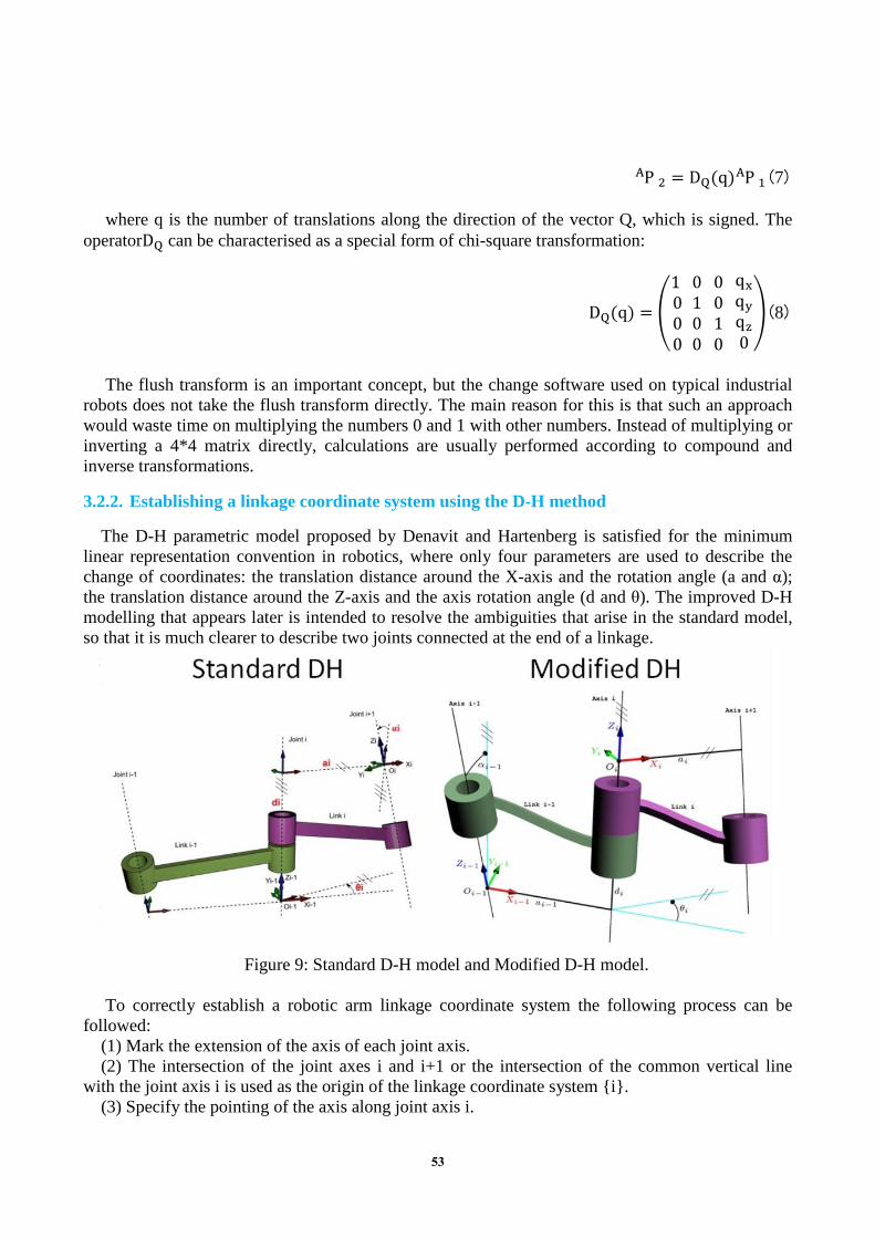
The D-H parametric model proposed by Denavit and Hartenberg is satisfied for the minimum linear representation convention in robotics, where only four parameters are used to describe the change of coordinates: the translation distance around the X-axis and the rotation angle (a and α); the translation distance around the Z-axis and the axis rotation angle (d and θ). The improved D-H modelling that appears later is intended to resolve the ambiguities that arise in the standard model, so that it is much clearer to describe two joints connected at the end of a linkage.

Figure 9: Standard D-H model and Modified D-H model.

To correctly establish a robotic arm linkage coordinate system the following process can be followed:

(1) Mark the extension of the axis of each joint axis. (2) The intersection of the joint axes i and i+1 or the intersection of the common vertical line

with the joint axis i is used as the origin of the linkage coordinate system {i}. (3) Specify the pointing of the axis along joint axis i.

53

(4) Specify the pointing of the axisXi along the common vertical line and, if the joint axes i and i+1 intersect, specify that the axisXi is perpendicular to the plane in which the joint axes i and i+1 lie.

(5) Determine the axisYi according to the right-hand rule. (6) Consider that the coordinate systems {0} and {1} coincide when and only when the first joint

variable is 0. There is no requirement that the origin and the direction of XN must be fixed in the co-ordinate system {N}, only that they are chosen so that the joint parameter is 0 if possible. Note: For steps 2 - 5, only two adjacent axes (joint axes i and i+1) are considered.

The solid joint coordinate system with each linkage allows the position and attitude of each linkage in the reference coordinate system to be represented, due to the fact that the tandem robot arm is connected by each linkage in a tandem fashion. The linkage transformation matrix for each joint can be found by using equations 7 to 9 and 8.

Standard DH:

𝑛𝑛−1 𝑇𝑇𝑛𝑛 =

⎝

⎛cosθn sinθn

0 0

−sinθncosαncosθncosαn

sinαn0

sinθnsinαn −cosθncosαn

cosαn 0

rncosθnrnsinθn

dn1 ⎠

⎞(9)

Modified DH:

𝑛𝑛−1 𝑇𝑇𝑛𝑛 =

⎝

⎛

cosθn sinθncosαn−1 sinθnsinαn−1

0

−sinθncosθncosαn−1cosθnsinαn−1

0

0 −sinαn−1 cosαn−1

0

an−1−dnsinαn−1dncosαn−1

1 ⎠

⎞(10)

From the above equation, we can in turn learn the linkage coordinate system for the end position

of the robot arm, which can be multiplied by each linkage coordinate system. 𝑇𝑇 = 𝑇𝑇1𝑇𝑇2𝑇𝑇3𝑇𝑇4𝑇𝑇5𝑇𝑇6(11)

3.2.3. Positive kinematic analysis

A positive kinematic solution for a robot arm with 6 degrees of freedom can be completed by referring to the following steps. (1) The linkage coordinate system of the robot arm with 6 degrees of freedom can be established by referring to the method for establishing the D-H linkage coordinate system. (2) The D-H parameters and joint variables are determined on the basis of this coordinate system. (3) Find the attitude matrix of the connecting rod. (4) Find the attitude matrix and kinematic equations of the end bar.

Based on the D-H parameter modelling method, the D-H parameters of the robotic arm were obtained as shown in the table.

Table 3-1 6 degrees of freedom robotic arm D-H parameter table Connecting rods θi/(°) d/mm a/mm α/(°) θ/(°)

1 θ1 0 0 0 0 2 θ2 0 a2=320 π/2 0 3 θ3 0 a3=975 0 0 4 θ4 d4=887 a4=200 π/2 0 5 θ5 0 0 -π/2 0 6 θ6 0 0 π/2 0

54

The transformation matrix of the joint unit can be built from the D-H model.

𝑇𝑇1 = �

cosθ1 −sinθ1

0 0

sinθ1cosθ1

00

0 0

1 0

0001

�(11)

𝑇𝑇2 = �

cosθ2 0

sinθ2 0

−sinθ20

cosθ20

0 −1 0 0

a2 0 0 1

�(12)

𝑇𝑇3 = �

cosθ3 sinθ3

0 0

−sinθ3cosθ3

00

0 0

1 0

a3001

�(13)

𝑇𝑇4 = �

cosθ4 −0

sinθ4 0

sinθ40

cosθ40

0 −1 0 0

a4−d4

01

�(14)

𝑇𝑇5 = �

cosθ5 −0

−sinθ5 0

sinθ50

−cosθ50

0 1 0 0

0001

�(15)

𝑇𝑇6 = �

cosθ6 0

sinθ6 0

−sinθ60

cosθ60

0 −1 0 0

0001

�(16)

Finally, the individual transformation matrices are multiplied together to obtain the total transformation matrix of the six-degree-of-freedom robot arm as:

𝑇𝑇总 = 𝑇𝑇1(θ1)𝑇𝑇2(θ2)𝑇𝑇3(θ3)𝑇𝑇4(θ4)𝑇𝑇5(θ5)𝑇𝑇6(θ6) = �

nx ny nz 0

ox oy oz0

ax ay az 0

pxpypz1

�(17)

Knowing the individual joint variables of the robot arm(),deriving the positive kinematics of the

arm will be simple and the results can be calculated using MATLAB.

nx=sin(theda6)*(cos(theda4)*sin(theda1)+sin(theda4)*(cos(theda1)*sin(theda2)*sin(theda3)-cos(theda1)*cos(theda2)*cos(theda3)))+cos(theda6)*(cos(theda5)*(sin(theda1)*sin(theda4)-

55

cos(theda4)*(cos(theda1)*sin(theda2)*sin(theda3)-cos(theda1)*cos(theda2)*cos(theda3)))-sin(theda5)*(cos(theda1)*cos(theda2)*sin(theda3)+cos(theda1)*cos(theda3)*sin(theda2))) (18)

ox=cos(theda6)*(cos(theda4)*sin(theda1)+sin(theda4)*(cos(theda1)*sin(theda2)*sin(theda3)-

cos(theda1)*cos(theda2)*cos(theda3)))-sin(theda6)*(cos(theda5)*(sin(theda1)*sin(theda4)-cos(theda4)*(cos(theda1)*sin(theda2)*sin(theda3)-cos(theda1)*cos(theda2)*cos(theda3)))-

sin(theda5)*(cos(theda1)*cos(theda2)*sin(theda3)+cos(theda1)*cos(theda3)*sin(theda2))) (19)

ax=sin(theda5)*(sin(theda1)*sin(theda4)-cos(theda4)*(cos(theda1)*sin(theda2)*sin(theda3)-cos(theda1)*cos(theda2)*cos(theda3)))+cos(theda5)*(cos(theda1)*cos(theda2)*sin(theda3)+cos(the

da1)*cos(theda3)*sin(theda2)) (20)

px=d4*(cos(theda1)*cos(theda2)*sin(theda3)+cos(theda1)*cos(theda3)*sin(theda2))-a4*(cos(theda1)*sin(theda2)*sin(theda3)-cos(theda1)*cos(theda2)*cos(theda3))+

a2*cos(theda1)+a3*cos(theda1)*cos(theda2) (21)

ny =-sin(theda6)*(cos(theda1)*cos(theda4)-sin(theda4)*(sin(theda1)*sin(theda2)*sin(theda3)-cos(theda2)*cos(theda3)*sin(theda1)))-

cos(theda6)*(cos(theda5)*(cos(theda1)*sin(theda4)+cos(theda4)*(sin(theda1)*sin(theda2)*sin(theda3)-

cos(theda2)*cos(theda3)*sin(theda1)))+sin(theda5)*(cos(theda2)*sin(theda1)*sin(theda3)+cos(theda3)*sin(theda1)*sin(theda2))) (22)

oy=sin(theda6)*(cos(theda5)*(cos(theda1)*sin(theda4)+cos(theda4)*(sin(theda1)*sin(theda2)*si

n(theda3)-cos(theda2)*cos(theda3)*sin(theda1)))+sin(theda5)*(cos(theda2)*sin(theda1)*sin(theda3)+cos(thed

a3)*sin(theda1)*sin(theda2)))-cos(theda6)*(cos(theda1)*cos(theda4)-sin(theda4)*(sin(theda1)*sin(theda2)*sin(theda3)-cos(theda2)*cos(theda3)*sin(theda1))) (23)

ay=cos(theda5)*(cos(theda2)*sin(theda1)*sin(theda3)+cos(theda3)*sin(theda1)*sin(theda2))-

sin(theda5)*(cos(theda1)*sin(theda4)+cos(theda4)*(sin(theda1)*sin(theda2)*sin(theda3)-cos(theda2)*cos(theda3)*sin(theda1))) (24)

py=d4*(cos(theda2)*sin(theda1)*sin(theda3)+cos(theda3)*sin(theda1)*sin(theda2))-

a4*(sin(theda1)*sin(theda2)*sin(theda3)-cos(theda2)*cos(theda3)*sin(theda1))+a2*sin(theda1)+a3*cos(theda2)*sin(theda1) (25)

nz=cos(theda6)*(sin(theda5)*(cos(theda2)*cos(theda3)-

sin(theda2)*sin(theda3))+cos(theda4)*cos(theda5)*(cos(theda2)*sin(theda3)+cos(theda3)*sin(theda2)))-sin(theda4)*sin(theda6)*(cos(theda2)*sin(theda3)+cos(theda3)*sin(theda2)) (26)

oz=-sin(theda6)*(sin(theda5)*(cos(theda2)*cos(theda3)-

sin(theda2)*sin(theda3))+cos(theda4)*cos(theda5)*(cos(theda2)*sin(theda3)+cos(theda3)*sin(theda2)))-cos(theda6)*sin(theda4)*(cos(theda2)*sin(theda3)+cos(theda3)*sin(theda2)) (27)

az=cos(theda4)*sin(theda5)*(cos(theda2)*sin(theda3)+cos(theda3)*sin(theda2))-

cos(theda5)*(cos(theda2)*cos(theda3)-sin(theda2)*sin(theda3)) (28)

56

pz=a4*(cos(theda2)*sin(theda3)+cos(theda3)*sin(theda2))-d4*(cos(theda2)*cos(theda3)-sin(theda2)*sin(theda3))+a3*sin(theda2) (29)

3.2.4. Inverse kinematic analysis

Inverse kinematic analysis is the opposite process to positive kinematic analysis. The inverse kinematic solution is achieved by first obtaining a data sheet of the pose of the end positions of the robot arm and then solving for the corresponding input angles of each joint. The inverse kinematic analysis is more important in the overall kinematics than the positive kinematic analysis. The presence or absence of a solution to the equation defines the working space of the arm. The absence of a solution means that the arm cannot achieve this desired position and attitude because the target point lies outside the working space of the arm, and it also directly affects the accuracy of the arm's motion and the precise characterisation of the control. There are two types of workspace, the dexterous workspace and the reachable workspace, both of which are very valuable. The former is defined as the area of space that can be reached by the arm's end-effector from either direction. The latter definition means that the robot arm can be reached in at least one direction, so that the dexterous space and the reachable space are contained and contained.

One of the difficulties in the study of multi-degree-of-freedom robotic arms is the existence of many sets of kinematic inverse solutions for multi-degree-of-freedom robotic arms. However, theoretical innovations have led to a large number of methods for solving the inverse solutions of multi-degree-of-freedom robotic arms. The best way to solve this problem is by defining the composition of the "solution" of the robot arm, since there is a general algorithm for solving linear systems of equations in positive kinematics, but not for non-linear systems. The solvable case of the robot arm is one where an algorithm can be identified to represent the joint variables and where the algorithm can identify all the variables to find the known position and associated pose. In the case of multiple solutions, the key to this definition is the requirement to be able to solve for all of them. This is why these numerical iterative procedures are not seriously considered when solving robot arm motion problems. The above divides the solution to the robot arm motion problem into two categories, one for closed solutions and the other for numerical solutions. The numerical solution is slower than the closed solution due to its iterative nature.

Here we do not go into a full unfolding study of it, but only find the joint angles by end-position settlement and then rely on the inverse solution function to intelligently output the best set of solutions from multiple sets of inverse solutions.

3.3. Fundamentals of robot kinematics

Using the above analysis of the robot arm with the D-H method parameters to build the model and using the Robotics toolbox of MATLAB the kinematics of the robot arm joints can be modelled. The kinematic simulation of a robot with 6 degrees of freedom is divided into two types, one with positive kinematics and the other with inverse kinematics. The former requires the angles and trajectories of the joints to be known and the kinematics to be used to analyse the trajectory of the end of the robot at each point in time. In the latter case, the end trajectory is known and the trajectory is solved by inverse kinematics.

The general kinematics, dynamics and trajectory planning of the robot arm can be achieved using the MATLAB Robotics Toolbox, which has a large number of functions and features [5][6], so the D-H parameters of the arm in Table 3-1 are modelled using the Link function in the Robotics Toolbox, which is called in the format L = Link(). Code 1 Robotics toolbox in Matlab to model the robot arm and solve the forward and inverse solutions.

57

Begin clear; clc; th(1) = 0; d(1) = 0; a(1) = 0; alp(1) = 0; th(2) = 0; d(2) = 0; a(2) = 3.20; alp(2) = pi/2; th(3) = 0; d(3) = 0; a(3) = 9.75; alp(3) = 0; th(4) = 0; d(4) = 8.87; a(4) = 2; alp(4) = pi/2; th(5) = 0; d(5) = 0; a(5) = 0; alp(5) = -pi/2; th(6) = 0; d(6) = 0; a(6) = 0; alp(6) = pi/2; L1 = Link([th(1), d(1), a(1), alp(1), 0], 'modified'); L2 = Link([th(2), d(2), a(2), alp(2), 0], 'modified'); L3 = Link([th(3), d(3), a(3), alp(3), 0], 'modified'); L4 = Link([th(4), d(4), a(4), alp(4), 0], 'modified'); L5 = Link([th(5), d(5), a(5), alp(5), 0], 'modified'); L6 = Link([th(6), d(6), a(6), alp(6), 0], 'modified'); robot = SerialLink([L1, L2, L3, L4, L5, L6]); robot.name='6-dof-robot'; robot.plot([0,0,0,0,0,0]); robot.display(); p=robot.fkine(th); q=robot.ikine(p); teach(robot); End.

Code. 1 Robotics toolbox in Matlab to model the robot arm and solve the forward and inverse solutions

Of these theta:joint angle, d:joint extension, a:joint offset (default 0), alpha:joint twist (default 0), offset:joint variable offset ( default 0). Running the Code 1 program, you will see the parameters of the robot arm model with the positive and negative solutions shown in Figure 10.

Figure. 10 Parameters and forward and inverse solutions of the robotic arm model based on the D-H method of simulation

58

Once the D-H robot arm model has been built, the forward and inverse kinematics can be solved using the Robotics toolbox using the SerialLink class of manipulation functions. Of these fkine represents the forward kinematic solution, and ikine is the inverse kinematic solution using an iterative approach. The joint angles are first specified, and then the end poses p are solved for according to our given joint theta. after obtaining the end poses p, the joint angles q are solved for by the given p.

4. Work space analysis of a multi-degree-of-freedom robot arm

4.1. Definition of work space

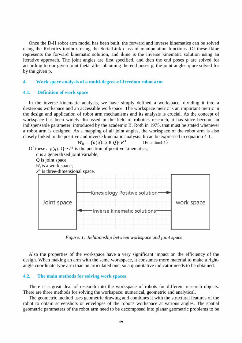
In the inverse kinematic analysis, we have simply defined a workspace, dividing it into a dexterous workspace and an accessible workspace. The workspace metric is an important metric in the design and application of robot arm mechanisms and its analysis is crucial. As the concept of workspace has been widely discussed in the field of robotics research, it has since become an indispensable parameter, introduced by the academic B. Roth in 1975, that must be stated whenever a robot arm is designed. As a mapping of all joint angles, the workspace of the robot arm is also closely linked to the positive and inverse kinematic analysis. It can be expressed in equation 4-1.

𝑊𝑊𝑅𝑅 = {𝑝𝑝(𝑞𝑞): 𝑞𝑞 ∈ 𝑄𝑄}∁𝑅𝑅3 （Equation4-1）

Of these，𝑝𝑝(𝑞𝑞): Q→𝑅𝑅3 is the position of positive kinematics; q is a generalized joint variable; Q is joint space; 𝑊𝑊𝑅𝑅is a work space; 𝑅𝑅3 is three-dimensional space.

Figure. 11 Relationship between workspace and joint space

Also the properties of the workspace have a very significant impact on the efficiency of the design. When making an arm with the same workspace, it consumes more material to make a right-angle coordinate type arm than an articulated one, so a quantitative indicator needs to be obtained.

4.2. The main methods for solving work spaces

There is a great deal of research into the workspace of robots for different research objects. There are three methods for solving the workspace: numerical, geometric and analytical.

The geometric method uses geometric drawing and combines it with the structural features of the robot to obtain screenshots or envelopes of the robot's workspace at various angles. The spatial geometric parameters of the robot arm need to be decomposed into planar geometric problems to be

59

used as the geometric solution for the robot arm. It is quite easy to apply this method when solving for the robot arm (especially when 𝛼𝛼𝑖𝑖 = 0𝑐𝑐𝑟𝑟 ± 90 ). The plane geometry tool can then be applied to find the joint angles, and since the robot arm is planar, we can use the plane geometry relations to solve it directly [7].

The analytical method is effective in finding the workspace, and although the engineering is complex, it is guaranteed to be effective as long as it is not used for more than 3 degrees of freedom. The implication is that the equations for the envelope boundary of the workspace are first derived before the work space is determined.

The numerical method depicts the boundary surface through a large number of boundary points, the acquisition of which relies on computer software capturing the characteristic points on the boundary surface of the robot arm's work space, and the capture of a large number of points is particularly dependent on the computer hardware. Even so, it has unparalleled advantages over the analytical method, particularly in complex robotic arms, which are not limited by degrees of freedom and are more effective in obtaining a graph of the workspace. Its widespread application came with the increasing availability of modern computer technology. On the basis of the development of stochastic theory, the Monte Carlo method emerged in order to solve the workspace of a multi-joint robot arm, where the generated random points are constructed on the workspace cloud of the robot arm and the image is displayed on the computer to obtain the contour of the work space [8].

4.3. Track generation

4.3.1. Path description and path generation

The motion of a robot arm is often thought of as the movement of a tool coordinate system {T} relative to a fixed coordinate system {S}. Thinking in this way is what most users of terminal robot systems do, and at the same time this way of describing paths and generating them brings many benefits to the user. It is not possible for the user to write complex time and space functions, so we want to make it possible for the user to specify the desired trajectory of the robot by performing simple commands and manipulate the robot through the system complete with detailed exact paths, time courses, velocity profiles, etc.

The representation of motion separate from all specific robot arms, end-effectors or workpieces is to specify paths according to the motion of the tool coordinate system corresponding to the fixed coordinate system. This brings the benefits of modularity when the same path description is applied to different robotic arms or to the same robotic arm with different tool sizes. It is therefore concluded that it is always feasible to determine and plan the motion with respect to a moving table by planning the motion with respect to a fixed coordinate system, and that time variation will also cause the definition of motion-time {S} to shift.

More details of the motion can be specified by giving a series of desired intermediate points in the path description which lie between the initial and final desired positions. So a series of transition positions and poses are usually described via intermediate points, and this path point expresses not only the position but also the positional information of the pose.

The desire to obtain smooth motion of the robot arm requires the introduction of smooth functions that are continuous and whose first-order derivatives are also continuous. In a few cases it is desired that the second order derivatives are also continuous. The wear and tear of the mechanism is mainly due to awkward, sharp movements which also excite the resonance of the robot arm. This is avoided by adding constraints on the spatial and temporal properties of the paths between intermediate points.

60

4.3.2. Planning methods for trajectories

The desired position and attitude of the instrumental coordinate system {T} with respect to the fixed coordinate system {S} is used to determine the path points. Solving for the desired joint angle corresponding to each point in the trajectory mainly applies inverse kinematic theory to obtain a smoothing function such that n joints pass through each intermediate point and median the target point. Since all joints take equal time to reach each path, all will also reach the midpoint at the same time, and the Cartesian position is obtained from the expectation of {T} at each intermediate point. In order to make the end motion of the robot arm smooth, the arm is often planned with certain constraints on the end velocity, acceleration, etc. A seven-segment S-curve is often used in industry for trajectory planning and is illustrated as follows:

Figure. 12 Seven-segment S-curve It has seven equally spaced time segments, namely acceleration, constant acceleration,

deceleration, uniform velocity, deceleration, constant acceleration and deceleration segments. The expressions for calculating the velocity of each segment are as follows, where J is the acceleration rate.

v(t) =

⎩⎪⎪⎪⎪⎨

⎪⎪⎪⎪⎧

12

J1t2, 0 ≤ t < t112

J1t2 + amax(t − t1), t1 ≤ t < t2vmax −

12

J1(t3 − t) 2, t2 ≤ t < t3vmax, t3 ≤ t < t4

vmax − (t − t4) 2, t4 ≤ t < t5vmax −

12

J1(t5 − t4) 2 − amax(t − t5), t5 ≤ t < t612

J1(t7 − t) 2, t6 ≤ t < t70, t7 ≤ t

（30）

The calculation of the equal parameters such as vmax in Equation 31 is derived as follows:

∆T = ti+1 − ti = tf−t07

（31）

L = 4vmax∆T（32）

v2 = v1 + amax∆T（33）

61

amax = 2v1∆T

（34）

vmax = v1 + v2 = 2v1 + amax∆T = 4v1 （35）

L = 16v1∆T → v1L

16∆T （36）

So in the end it is only necessary to know the end displacement L and the required time T to

calculate the entire trajectory planning curve. Trajectory planning can be divided into joint trajectory planning and Cartesian space trajectory

planning, the difference between them is that the physical quantities transform into different relationships as a function of time. The physical quantities in joint space trajectory planning are joint variables, which are then constrained to angular velocity and angular acceleration, whereas Cartesian space trajectory planning is the displacement, velocity and acceleration of the robot's end in Cartesian space. Because the calculations in joint space are easy and do not have a continuous correspondence with the Cartesian coordinates, the singularity problem of the mechanism does not occur. Because of these advantages it is very commonly used and is often employed.

Here it is used for trajectory planning in a reduced dimensional way using cubic polynomial and quintuple polynomial interpolation, respectively, and here the object of study is a one-dimensional trajectory, which is applied by comparing the results between them on merit.

Firstly, the cubic polynomial interpolation method is investigated with four coefficients to be determined θ(t) = θ0，θ(tf) = θf， θ̇(0) = 0， θ̇(tf) = 0 respectively. The first two are two constraints on the value of the function that can be obtained from the initial and final values, while the last two are needed to ensure that the joint velocity is continuous, that is to say that the joint velocity is zero at the initial and termination moments, and that constraints can be given on both the angle and angular velocity of the start and target points. These four constraints uniquely determine a cubic polynomial of the following form.

θ(t) = a0 + a1t + a2t2 + a3t3(37)

The joint velocities and accelerations corresponding to this path are therefore

θ̇(t) = a1 + 2a2t + 3a3t2(38)

θ̈(t) = 2a2 + 6a3t(39)

The four constraints are then substituted into equations 4-8 to 4-10 to give

⎩⎨

⎧θ0 = a0

θf = a0 + a1tf + a2tf2 + a3tf30 = a1

0 = 𝑎𝑎1 + 2𝑎𝑎2 + 3𝑎𝑎3𝑡𝑡𝑓𝑓2(40)

62

Finally solving for in Equation 4-11 gives

⎩⎪⎨

⎪⎧

a0 = θ0a1 = 0

a2 = 3tf3

(θf − θ0)

a3 = − 2tf3

(θf − θ0)

(41)

This solution is based on the starting joint angular velocity and the ending joint angular velocity both being zero. If we set the constrained starting velocity to v0 and the ending velocity to vf using MATLAB, where the starting and ending positions, time, velocity and acceleration are specified as shown in the table.

Table 4-1 Specifying start/stop position, time, speed and acceleration Connecting rods Location/m Speed/(m/s) Acceleration/(m/s2) Time/s

1 0 0 0 0

2 50 10 20 3

3 150 20 30 6

4 100 -15 -20 12

5 0 0 0 14

Using the data in Table 4-1 in Code 4-1, the MATLAB part of the code is as follows. Begin %Three-dimensional polynomial interpolation clear; clc; q_array=[0,50,150,100,0];%Specify starting and ending position t_array=[0,2,4,8,10];%Specify start and end times v_array=[0,10,20,-15,0];%Specify starting and stopping speed t=(t_array(1));q=(q_array(1));v=(v_array(1));a=(0);%Initial

state for i=1:1:length(q_array)-1%Time for each planning section a0=q_array(i); a1=v_array(i); a2=(3/(t_array(i+1)-t_array(i))^2)*(q_array(i+1)-q_array(i))-

(1/(t_array(i+1)-t_array(i)))*(2*v_array(i)+v_array(i+1)); a3=(2/(t_array(i+1)-t_array(i))^3)*(q_array(i)-q_array(i+1))+(1/(t_array(i+1)-t_array(i))^2)*(v_array(i)+v_array(i+1)); ti=t_array(i)+0.001:0.001:t_array(i+1); qi=a0+a1*(ti-t_array(i))+a2*(ti-t_array(i)).^2+a3*(ti-

t_array(i)).^3; vi=a1+2*a2*(ti-t_array(i))+3*a3*(ti-t_array(i)).^2; ai=2*a2+6*a3*(ti-t_array(i)); t=[t,ti];q=[q,qi];v=[v,vi];a=[a,ai]; end subplot(3,1,1),plot(t,q,'r'),xlabel('t/s'),ylabel('p/m');hold

on;plot(t_array,q_array,'o','color','r'),grid on;

63

subplot(3,1,2),plot(t,v,'b'),xlabel('t/s'),ylabel('v/(m/s)');holdon;plot(t_array,v_array,'*','color','r'),grid on; subplot(3,1,3),plot(t,a,'g'),xlabel('t/s'),ylabel('a/(m/s^2)');h

old on; End.

Code 2-1 Third polynomial interpolation code section The results of the run are as follows.

Figure. 13 MATLAB implementation of cubic polynomial interpolation effect

The same is true for the five polynomial interpolation method, except that there are two more coefficients to be determined than in the three polynomial interpolation method and constraints can be given for both the starting and target states. As can be seen from the comparative analysis of the curves in Figure. 14, there are no jumps and the simulation results are smooth curves, which prevent the joint motor from being shocked. Although the five-polynomial interpolation method is much more computationally intensive, the time cost is negligible as it is not real-time planning. In terms of the smoothness of the planned trajectory, therefore, the quintuple polynomial interpolation method is more effective.

Figure. 14 The effect of triple polynomial interpolation versus quintuple polynomial interpolation

4.4. Second Section

This section must be in one column.

64

5. Analysis of MATLAB simulation results

5.1. Simulation of trajectory planning for a six-degree-of-freedom robot arm

This robotic arm trajectory is planned using a five-polynomial interpolation method.

Figure. 15 Outputting parameters with the display function

Figure. 16 Position of each joint

65

Figure. 17 Angular velocity of each joint

Figure. 18 Angular acceleration of each joint

66

Figure. 19 Spatial trajectory of a six-degree-of-freedom robot arm

With the simulation results of the trajectory planning of the six-degree-of-freedom robot arm, we obtain its spatial trajectory movements and display them as curves. As can be seen in Figure. 19, the arm successfully reaches the desired position, which shows that the design of the arm is feasible and reasonable. The entire trajectory and process is shown in Fig. 16 to Fig. 18, from which the relationship between the state of each joint and time can be analysed, showing that the angular velocity and angular acceleration of the joint and the position curve change smoothly and continuously. Therefore, the absence of sudden jumps effectively prevents the arm from being shocked and causing wear to its components, and the velocity and acceleration at points A and B can be effectively bound to zero.

5.2. Summary

The analysis and simulation of the robotic arm shows the importance of the kinematics and dynamics of the robotic arm, and its analysis is very helpful for the structure of the robotic arm. Although this article is mainly a simulation study on the basic kinematics and spatial trajectory, it is the most important part of the overall robotic arm design and control that is inseparable. The control of the robot arm itself relies on sensors to enhance its functionality, and subsequent optimisation is useless if the design itself lacks rationality and efficiency. The robotic arm is the prototype of a robot, and the system can be broadly divided into four parts. These are the arm, the end-effector, the sensors and inductors and the controller. The main design considerations here are those that are likely to have the greatest impact on the design, and this is the basis on which more high level design solutions can be considered. For example, the optimisation of the arm's structural parameters, specific and relevant types of improvements for specific tasks, etc.

67

Acknowledgements

As the work on my dissertation design continued to progress, it came to an end in the blink of an eye. Looking back on my undergraduate studies, I have experienced many hardships and gained a lot from the help of my teachers and classmates. First of all, I would like to thank my supervisor, Ms Wang Jun, for her careful guidance and assistance, not only in the design process of this thesis, but also for her advice in my postgraduate application. She has been very patient in all aspects of the thesis, from the selection of the topic to the revision of the topic and the conceptualisation to the final draft. I would also like to thank all the teachers who helped me with my postgraduate application, without their selfless help I would not have been able to get the admissions I wanted. The design was initially to control a multi-degree-of-freedom robot arm to achieve multi-functional work, but in order to expand my knowledge of robotics and lay the foundation for my future studies, I chose to change the direction of the design to simulate the kinematics and spatial trajectory of a multi-degree-of-freedom robot arm. I would also like to thank my friends who provided me with logical ideas and reference materials to complete this thesis. Finally, I hope to use this as a basis for further exploration of intelligent robotics in the future, and to make further breakthroughs.

References

[1] Wang Daina. A study of robot subjectivity(Ji Qi Ren Zhu Ti Xing Wen Ti Yan Jiu)[D]. Chengdu: Chengdu University of Technology, 2018.

[2] Chen Jun. Research on real-time simulation system for multi-degree-of-freedom robotic arm(Duo Zi You Du Ji Xie Bi Shi Shi Fang Zhen Xi Tong Yan Jiu)[D]. Harbin: Harbin Engineering University, 2012.

[3] Edelman, B. J., Meng, J., Suma, D., Zurn, C., Nagarajan, E., Baxter, B. S., Cline, C. C., & He, B. (2019). Noninvasive neuroimaging enhances continuous neural tracking for robotic device control. Science Robotics, 4(31), eaaw6844. https://doi.org/10.1126/scirobotics.aaw6844

[4] Xu Kou. Inverse kinematic solution and trajectory planning of a six-degree-of-freedom robotic arm(Liu Zi You Du Ji Xie Bi De Ni Yun Dong Xue Qiu Jie Yu Gui Ji Gui Hua Yan Jiu)[D]. Guangzhou: Guangdong University of Technology, 2016.

[5] Ma Yuhao. Six-degree-of-freedom robotic arm obstacle avoidance trajectory planning and control algorithm research(Liu Zi You Du Ji Xie Bi Bi Zhang Gui Ji Ji Kong Zhi Suan Fa Yan Jiu)[D]. University of Chinese Academy of Sciences, 2019.

[6] Zuo Fuyong, Hu Xiaoping, Xie Ke, et al. SCARA robot trajectory planning and simulation based on MATLAB Robotics toolbox(Ji Yu MATLAB Robotics Gong Ju Xiang De SCARA Ji Qi Ren Gui Ji Gui Hua Yu Fang Zhen)[J]. Haapasalo, Xiang Tan: Journal of Hunan University of Science and Technology, 2012(2):43-46.

[7] Lee, C. s. g., & Ziegler, M. (1984). Geometric approach in solving inverse kinematics of PUMA robots. IEEE Transactions on Aerospace and Electronic Systems, AES-20(6), 695 – 706. https://doi.org/10.1109/taes.1984.310452

[8] Wang Yongjie. Optimisation of structural parameters for multi-degree-of-freedom robotic arms(Duo Zi You Du Ji Xie Bi Jie Kou Can Shu You Hua)[D]. Beijing Institute of Technology, 2016.

[9] Denavit, J. and Hartenberg, R.S. (1955) A Kinematic Notation for Lower-Pair Mechanisms Based on Matrices. ASME Journal of Applied Mechanics, 77, 215-221.

[10] Li Baofeng, Sun Hanxu, Jia Qingxuan, et al. Space robot workspace calculation based on Monte Carlo method(Ji Yu Meng Te Ka Luo Fa De Kong Jian Ji Qi Ren Gong Zuo Kong Jian Ji Suan)[J]. Journal of Spacecraft Engineering, 2012,20(4):79-85.

[11] Roth B. Performance Evaluation of Manipulators from a Kinematic Viewpoint[J]. National Bureau of Standards Workshop on Performance Evaluation of Manipulators, 1975.

[12] Cao Yi, Wang Shuxin, Qiu Yan, et al. Design of a microsurgical robot for flexible work spaces(Mian Xiang Ling Huo Gong Kong Jian De Xian Wei Wai Ke Shou Shu Ji Qi Ren She Ji)[J]. Robotics journals, 2005,27(3):220-225.

[13] Abdel-Malek, K., & Yeh, H.-J. (1997). Analytical boundary of the workspace for general3-dof mechanisms. The International Journal of Robotics Research, 16(2), 198–213. https://doi.org/10.1177/027836499701600206

68

[14] Chen Zhangping, Diao Yan, Yao Lin, et al. Minimally invasive surgical robot workspace analysis(Wei Chuang Shou Shu Ji Qi Ren Gong Zuo Kong Jian Fen Xi)[J]. Journal of Mechanical Science and Technology, 2010,27(10):70-72.

[15] Jouybari, B. R., Osgouie, K. G., & Meghdari, A. (2014). Optimization of kinematic redundancy and workspace analysis of a dual-arm cam-lock robot. Robotica, 34(1), 23–42. https://doi.org/10.1017/s0263574714000423

[16] Zhou Aiguo, Zhou Fei, Nv Gang, et al. Kinematics and workspace analysis of an articulated arm CMMJ(Guan Jie Bi Shi Zuo Biao Ce Liang Ji De Yun Dong Xue Yu Gong Zuo Kong Jian Fen Xi)[J]. Journal of Mechanical Drives, 2019.10.

[17] Craig, J. J. (2017). Introduction to robotics: Mechanics and control. Prentice Hall. [18] Yang Zhongrui. Kinematics and trajectory planning research for industrial robots(Gong Ye Ji Qi Ren De Yun

Dong Xue Yu Gui Ji Gui Hua Yan Jiu)[D]. Chengdu: Xihua University, 2020. [19] Yang Yijun, Chen Xunbing. Kinematic analysis of a general-purpose six-degree-of-freedom industrial robot(Tong

Yong Xing Liu Zi You Du Gong Ye Ji Qi Ren De Yun Dong Xue Fen Xi)[D]. Guangzhou: Guangdong University of Technology, 2017.

[20] Tian Guofu, Jiang Chunxu. Kinematic analysis of industrial robots in MATLAB Robotics(Gong Ye Ji Qi Ren Zai MATLAB Robotics Zhong De Yun Dong Xue Fen Xi)[D]. Heavy Machinery Journal, 2019.

[21] Li Wei. Six degree of freedom articulated robot control system development(Liu Zi You Du Guan Jie Shi Ji Qi Ren Kong Zhi Xi Tong Kai Fa)[D]. Shanghai: East China University of Science and Technology, 2014.

69