multi core computing and mri -...

Multi-Core Computing Jan 2010 Richard Ansorge

Multi Core Computing

Richard Ansorge January 2010


Moore’s Law?

• Exponential growth in computing power since early 1960’s.

• Single processor power peaked in 1990’s• Many calculations limited by memory

bandwidth not CPU• PC clusters used since mid 1990’s• Multicore PC chips now entry level• Graphics cards have 100’s of cores


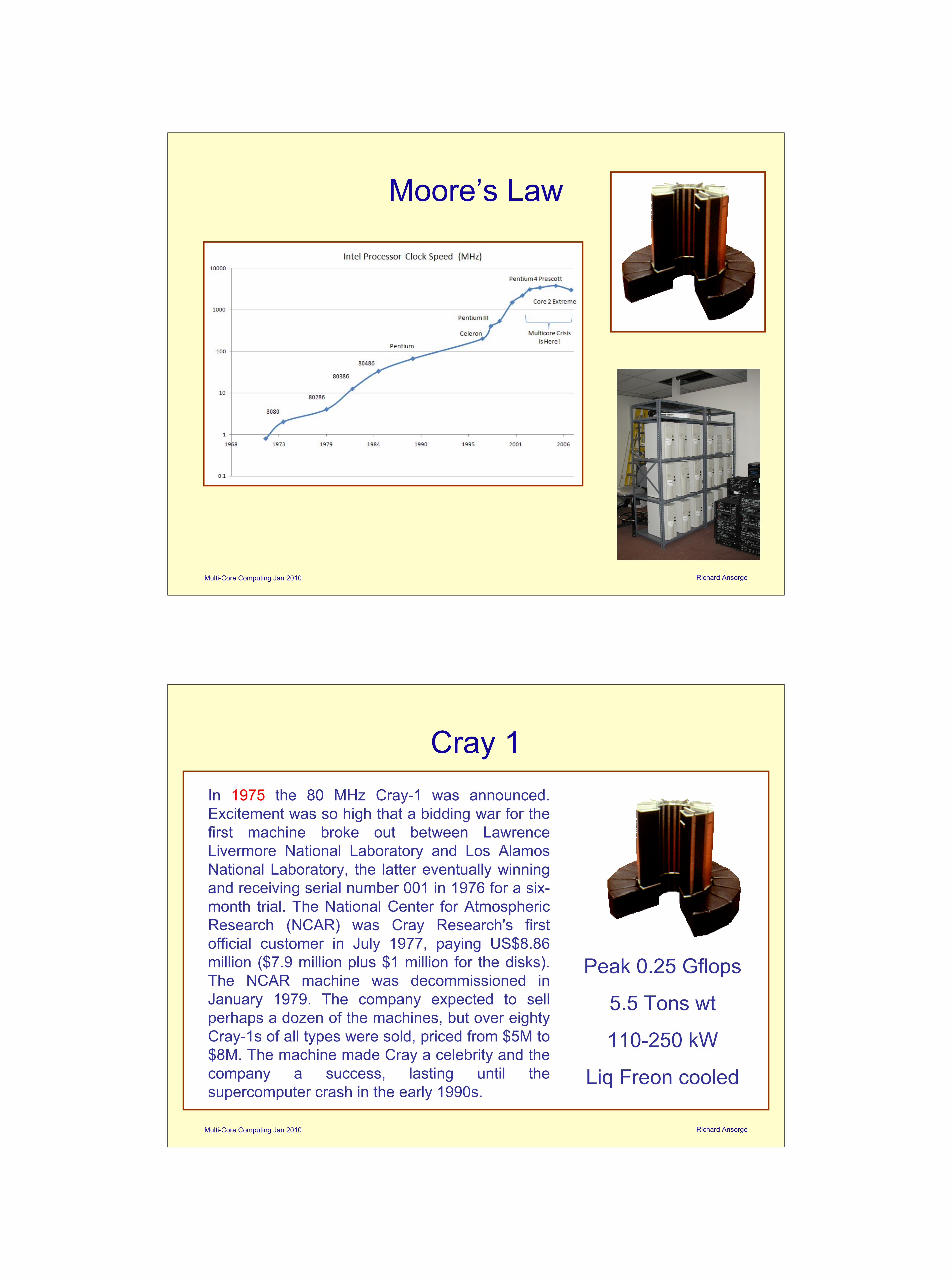
Moore’s Law


Cray 1In 1975 the 80 MHz Cray-1 was announced. Excitement was so high that a bidding war for the first machine broke out between Lawrence Livermore National Laboratory and Los Alamos National Laboratory, the latter eventually winning and receiving serial number 001 in 1976 for a six-month trial. The National Center for Atmospheric Research (NCAR) was Cray Research's first official customer in July 1977, paying US$8.86 million ($7.9 million plus $1 million for the disks). The NCAR machine was decommissioned in January 1979. The company expected to sell perhaps a dozen of the machines, but over eighty Cray-1s of all types were sold, priced from $5M to $8M. The machine made Cray a celebrity and the company a success, lasting until the supercomputer crash in the early 1990s.

Peak 0.25 Gflops

5.5 Tons wt

110-250 kW

Liq Freon cooled


Distributed Computing

• If lucky can just run same code on each processing core; e.g. event simulation.

• But be careful to use 64 bit random number generator and ensure different sequences.

• Otherwise cores share data:– shared memory machine– local memories + interconnect – latency and bandwidth constraints


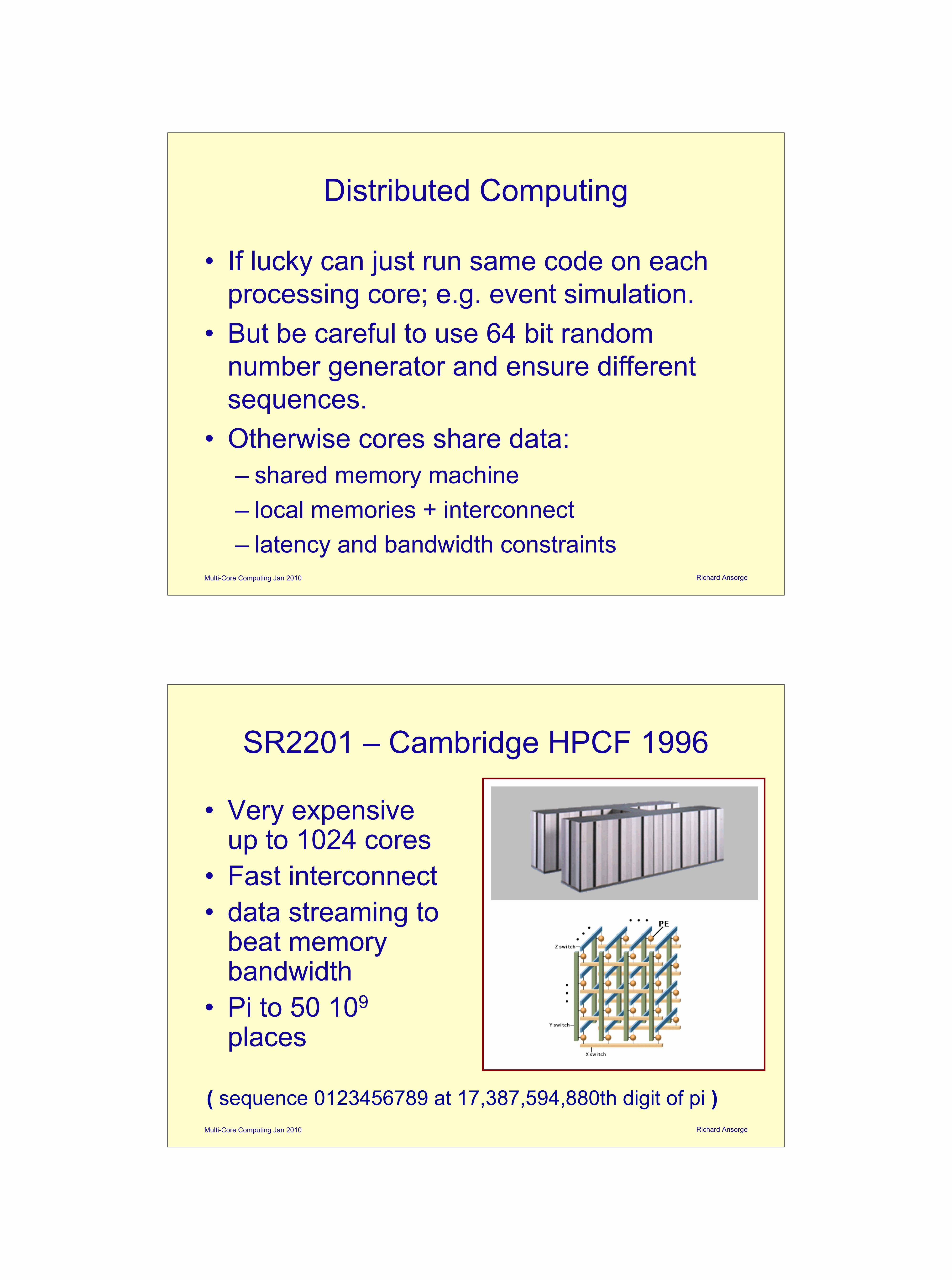
SR2201 – Cambridge HPCF 1996

• Very expensive up to 1024 cores

• Fast interconnect• data streaming to

beat memory bandwidth

• Pi to 50 109

places

( sequence 0123456789 at 17,387,594,880th digit of pi )


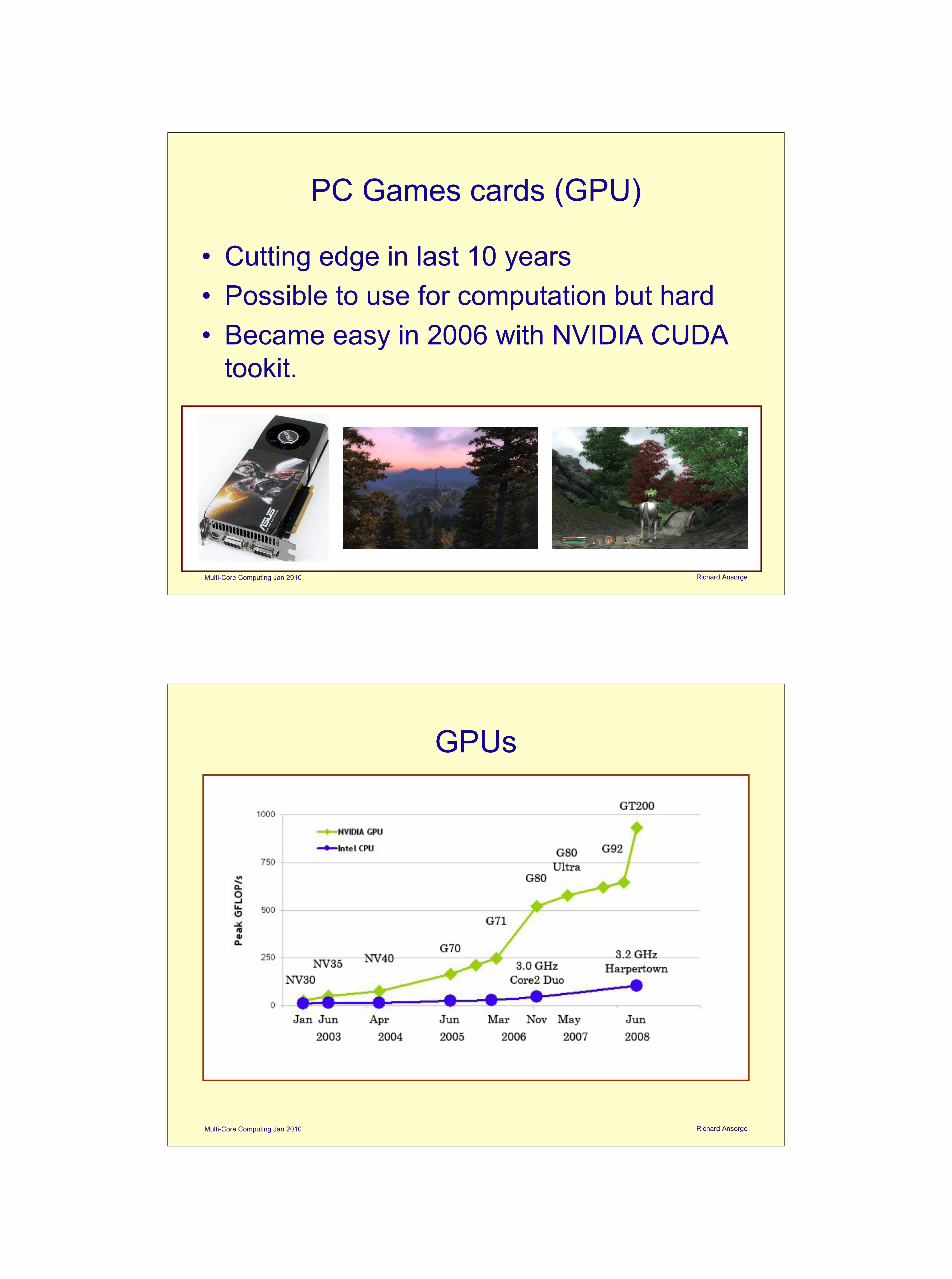
PC Games cards (GPU)

• Cutting edge in last 10 years• Possible to use for computation but hard• Became easy in 2006 with NVIDIA CUDA

tookit.


GPUs


GPUs – Also Memory Bandwidth


Available Resources

• Own PC (perhaps multi-core and with GPU)• BSS server (8 cores + Tesla GPU)• Camgrid (ask Owen)• Cambridge HPC ask me• National Centre• etc...


Programming Recommendations

• MPI (message passing interface) for conventional cores– portable– well supported and documented– introduces idea of collective operations

• CUDA for NVIDIA GPUs– in many ways similar but with global memory space

and limited communication– scales to huge numbers of threads– cluster of multiprocessors


MPI

• Function Library• Same program code runs on all cores• 100’s of functions but you only need a tiny

number• Rarely need the send/receive calls used in

most introductions!• Learn the collective operations.


Hello World

#include <stdio.h>#include <mpi.h>

int main(int argc, char *argv[]) {int node, nodes;

MPI_Init(&argc, &argv);MPI_Comm_size(MPI_COMM_WORLD, &nodes);MPI_Comm_rank(MPI_COMM_WORLD, &node);

printf("Hello mpi world, I am node %d out of %d in all\n", node,nodes);

MPI_Finalize();return 0;

}

#include <stdio.h>

int main(int argc, char *argv[]) {

printf("Hello World\n");return 0;

} MPI Headernode specifies which core I am out of a total of nodes. Typically use to coordinate calculation.

eg if(node==0) printf(“stuff\n”);

standard initialisation

standard close


Run using MPICH2


Matrix Multiply Example

for N x N matrices need N3

multiply-adds (mad)

1Nkij ik kjA BC ==

Share rows of A across nodes.

Full copy of B required on all nodes

But only N/nodes rows of A and C required on one node

=×A B C


MatMul Declarations// simple matrix multipy on host #include <stdlib.h>#include <stdio.h>#include <string.h>#include <math.h>#include <time.h>

typedef struct {int cols;int rows;int stride;float* m;

} Matrix;

// prototypesvoid hostMatMul(const Matrix A, const Matrix B, Matrix C);void randomInit(float* data, int size);clock_t watch (int it);


MatMul Mainint main(int argc,char *argv[]){

if(argc <2) {printf("usage simpleMatMul <size>\n");return 0;

}watch(-1); // start timerswatch(1);Matrix A; Matrix B; Matrix C;

int msize = 16*atoi(argv[1]);

A.cols = A.rows = A.stride = msize;B.cols = B.rows = B.stride = msize;C.cols = C.rows = C.stride = msize;

A.m = new float[msize*msize]; randomInit(A.m,msize*msize);B.m = new float[msize*msize]; randomInit(B.m,msize*msize);C.m = new float[msize*msize];

hostMatMul(A,B,C);

printf("Timings for C=A*B for %d x %d matricies\n",msize,msize);watch(-2);

return 0;}


Mat Mul Code - Host

void hostMatMul( Matrix A,Matrix B,Matrix C ){

watch(2);for(int row=0;row<A.cols;row++) for(int col=0;col<B.rows;col++){

float sum=0.0f;for(int k=0;k<A.cols;k++) sum += A.m[row*A.cols+k]*B.m[k*B.cols+col];C.m[row*A.cols+col] = sum;

}return;

}


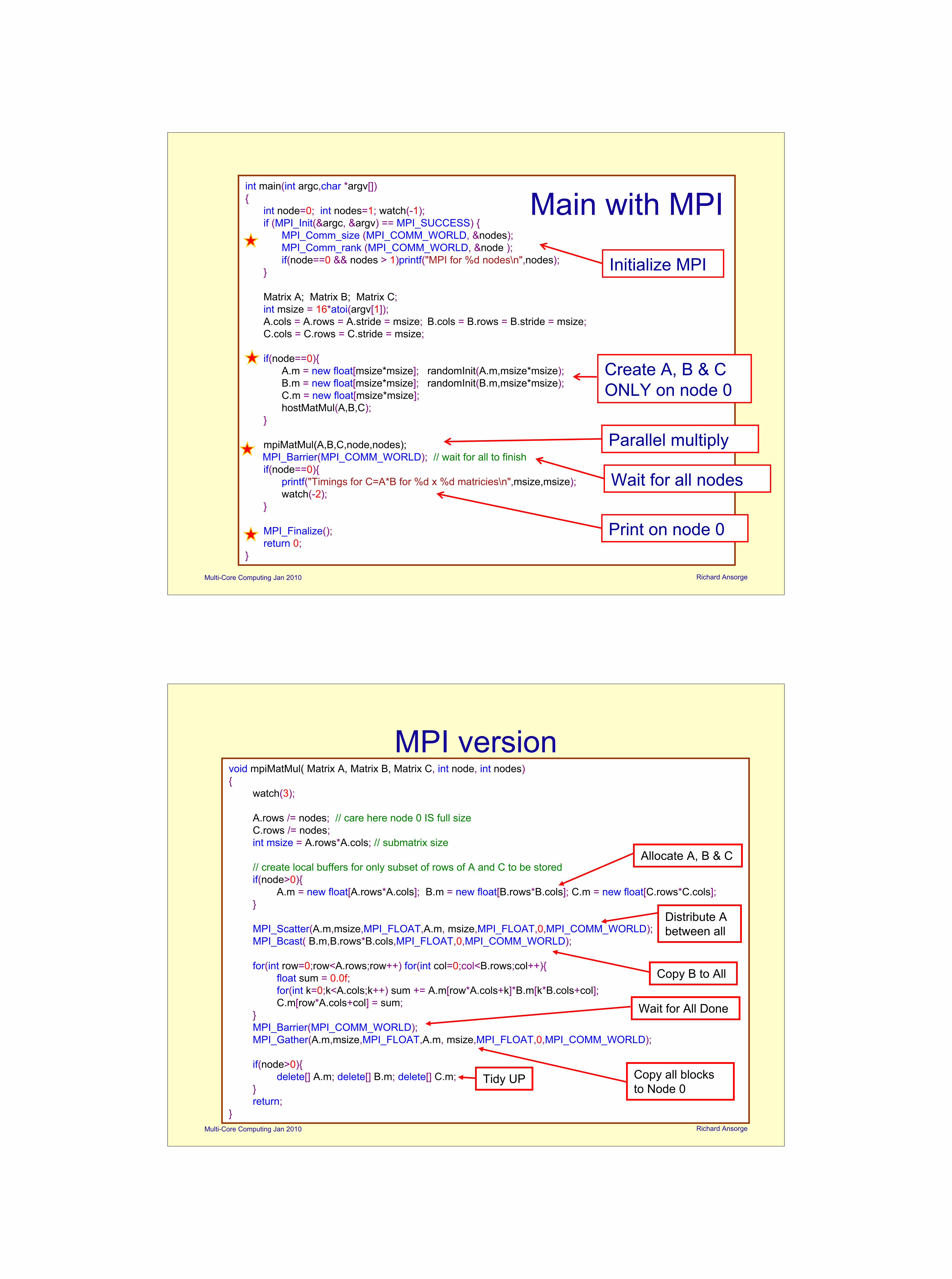
int main(int argc,char *argv[]){

int node=0; int nodes=1; watch(-1);if (MPI_Init(&argc, &argv) == MPI_SUCCESS) {

MPI_Comm_size (MPI_COMM_WORLD, &nodes);MPI_Comm_rank (MPI_COMM_WORLD, &node );if(node==0 && nodes > 1)printf("MPI for %d nodes\n",nodes);

}

Matrix A; Matrix B; Matrix C;int msize = 16*atoi(argv[1]);A.cols = A.rows = A.stride = msize; B.cols = B.rows = B.stride = msize;C.cols = C.rows = C.stride = msize;

if(node==0){A.m = new float[msize*msize]; randomInit(A.m,msize*msize);B.m = new float[msize*msize]; randomInit(B.m,msize*msize);C.m = new float[msize*msize];hostMatMul(A,B,C);

}

mpiMatMul(A,B,C,node,nodes);MPI_Barrier(MPI_COMM_WORLD); // wait for all to finishif(node==0){

printf("Timings for C=A*B for %d x %d matricies\n",msize,msize);watch(-2);

}

MPI_Finalize();return 0;

}

Main with MPI

Initialize MPI

Create A, B & C ONLY on node 0

Parallel multiply

Wait for all nodes

Print on node 0


MPI versionvoid mpiMatMul( Matrix A, Matrix B, Matrix C, int node, int nodes){

watch(3);

A.rows /= nodes; // care here node 0 IS full sizeC.rows /= nodes;int msize = A.rows*A.cols; // submatrix size

// create local buffers for only subset of rows of A and C to be storedif(node>0){

A.m = new float[A.rows*A.cols]; B.m = new float[B.rows*B.cols]; C.m = new float[C.rows*C.cols];}

MPI_Scatter(A.m,msize,MPI_FLOAT,A.m, msize,MPI_FLOAT,0,MPI_COMM_WORLD);MPI_Bcast( B.m,B.rows*B.cols,MPI_FLOAT,0,MPI_COMM_WORLD);

for(int row=0;row<A.rows;row++) for(int col=0;col<B.rows;col++){float sum = 0.0f;for(int k=0;k<A.cols;k++) sum += A.m[row*A.cols+k]*B.m[k*B.cols+col];C.m[row*A.cols+col] = sum;

}MPI_Barrier(MPI_COMM_WORLD);MPI_Gather(A.m,msize,MPI_FLOAT,A.m, msize,MPI_FLOAT,0,MPI_COMM_WORLD);

if(node>0){delete[] A.m; delete[] B.m; delete[] C.m;

}return;

}

Wait for All Done

Copy all blocks to Node 0

Copy B to All

Distribute A between all

Allocate A, B & C

Tidy UP


Test on old 2-core PC

Broadcast (copy to all)


NB MPI can be smart, using switch optimally

Scatter – share data between nodes


Gather – collect data to one node


Reduce, e.g. sum across nodes


Others



CUDA- Recent NVIDIA GPUs• Cards have up to 30 multiprocessors• Each multiprocessor has 8 cores• Each multiprocessor runs a thread block of

up to 512 threads “simultaneously”• Thread blocks can share limited fast

memory• No communication between thread blocks• CUDA runs sufficient tread blocks to

complete task


CUDA DeviceShared memory is local to multiprocessor and is not visible to host. Shared memory does not persistThe other memories are global and are visible to host and are persistent across multiple kernel executions. SIMD model.


CUDA Device Query (st1)


CUDA Device Query (my BSS PC)


CUDA Device Query (Games PC)


CUDA ProgramCUDA program runs on single host core. Typically:•sends data to device memories.•launches one or more kernels on device.•collects final results back from device global memory.•A kernel is a piece of C like code which is run by many threads.


CUDA Matrix Multiply first version

Use separate threads for each element Cij in matrix product

C= A*B

Thus N2 threads.

Each thread block will correspond to a 16x16 sub matrix of C.

(NB 16x16 is often a very good choice)


Kernel Code// Matrix multiplication kernel called by devMatrixMul()__global__ void MatMulKernel( Matrix A, Matrix B, Matrix C ){

// Each thread computes one element of C accumulating results into sumfloat sum = 0.0f;int row = blockIdx.y * blockDim.y + threadIdx.y;int col = blockIdx.x * blockDim.x + threadIdx.x;

for (int k=0;k<A.cols;++k) sum += A.m[row*A.cols+k]*B.m[k*B.cols+col];C.m[row*C.cols+col] = sum;

}

void hostMatMul( Matrix A,Matrix B,Matrix C ){

watch(2);for(int row=0;row<A.cols;row++) for(int col=0;col<B.rows;col++){

float sum=0.0f;for(int k=0;k<A.cols;k++) sum += A.m[row*A.cols+k]*B.m[k*B.cols+col];C.m[row*A.cols+col] = sum;

}return;

}

local variable in register thus fast

A, B and C are allocated by Host in device global memory – thus slow.

Find which element of C this thread needs to calculate. The variables on RHS are maintained by CUDA

Same function arguments! Set by Host but data pointer is to device memory


void devMatMul(Matrix A, Matrix B, Matrix C){

// Copy A and B to devA and devB in device memoryMatrix devA;devA.cols = A.cols; devA.rows = A.rows; devA.stride = A.stride;size_t size = A.cols * A.rows * sizeof(float);cudaMalloc((void**)&devA.m, size);cudaMemcpy( devA.m, A.m, size ,cudaMemcpyHostToDevice);

Matrix devB;devB.cols = B.cols; devB.rows = B.rows; devB.stride = B.stride;size = B.cols * B.rows * sizeof(float);cudaMalloc((void**)&devB.m, size);cudaMemcpy( devB.m, B.m, size ,cudaMemcpyHostToDevice);

// Allocate devC in device memory no need to copyMatrix devC;devC.cols = C.cols; devC.rows = C.rows; devC.stride = C.stride;size = C.cols * C.rows * sizeof(float);cudaMalloc((void**)&devC.m, size);

dim3 dimBlock(16, 16);dim3 dimGrid(B.cols/dimBlock.x, A.rows/dimBlock.y);

// Invoke kernelMatMulKernel<<<dimGrid, dimBlock>>>(devA, devB, devC);cudaThreadSynchronize();// copy result back to hostcudaMemcpy( C.m, devC.m, size, cudaMemcpyDeviceToHost);cudaThreadSynchronize();

// Free device memorycudaFree(devA.m); cudaFree(devB.m); cudaFree(devC.m);

}

CUDA host code

CUDA kernel call, note arguments

Create copies of A, B & C in device memory

define thread blocks

Copy answer back to host


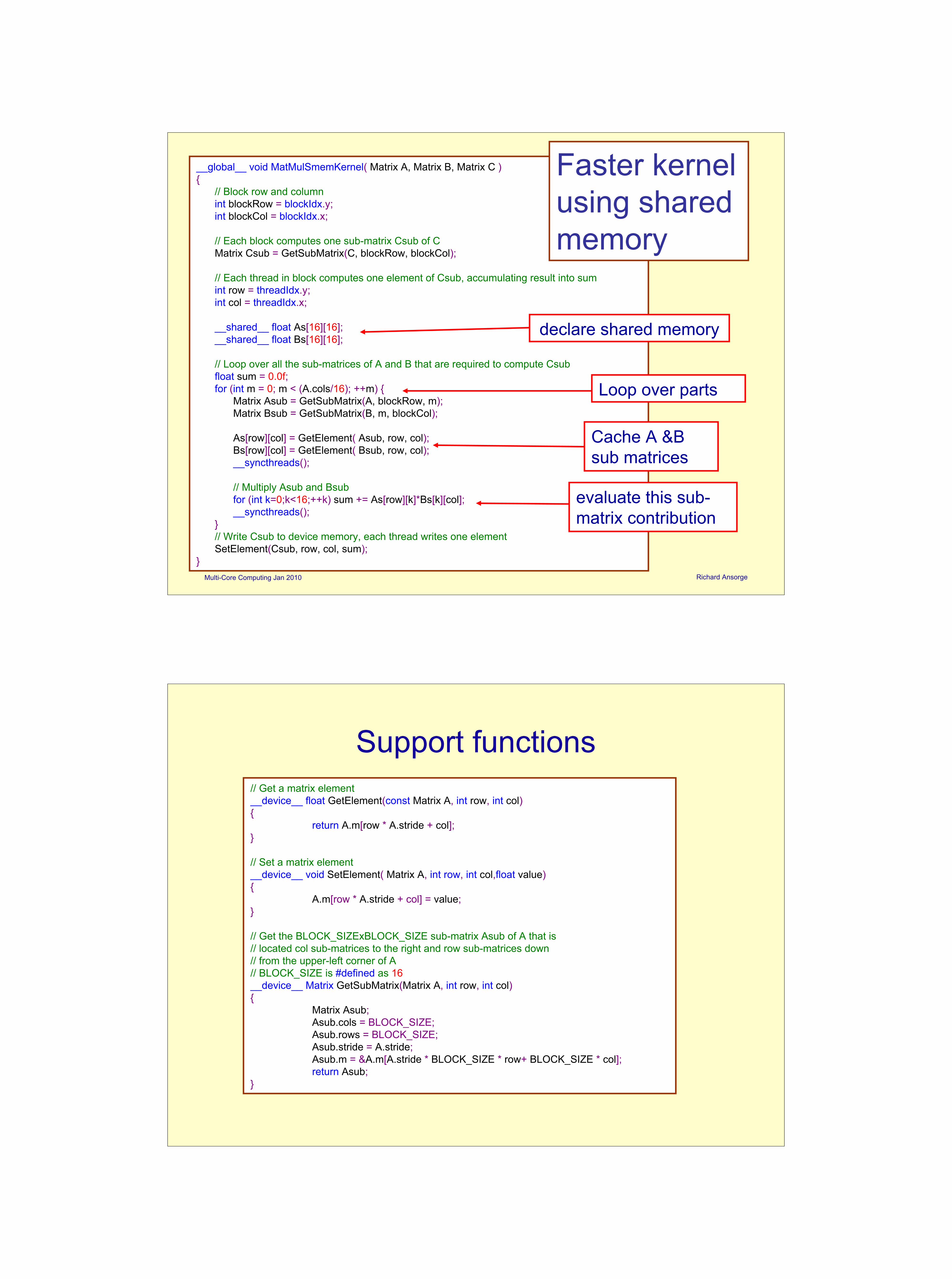
Faster kernel using shared memory

Each thread block uses shared memory to cache a 16x16 sub-blocks of the matrices. This improves performance, especially when addressing B with a large stride.


__global__ void MatMulSmemKernel( Matrix A, Matrix B, Matrix C ){

// Block row and columnint blockRow = blockIdx.y;int blockCol = blockIdx.x;

// Each block computes one sub-matrix Csub of CMatrix Csub = GetSubMatrix(C, blockRow, blockCol);

// Each thread in block computes one element of Csub, accumulating result into sumint row = threadIdx.y;int col = threadIdx.x;

__shared__ float As[16][16];__shared__ float Bs[16][16];

// Loop over all the sub-matrices of A and B that are required to compute Csubfloat sum = 0.0f;for (int m = 0; m < (A.cols/16); ++m) {

Matrix Asub = GetSubMatrix(A, blockRow, m);Matrix Bsub = GetSubMatrix(B, m, blockCol);

As[row][col] = GetElement( Asub, row, col);Bs[row][col] = GetElement( Bsub, row, col);__syncthreads();

// Multiply Asub and Bsubfor (int k=0;k<16;++k) sum += As[row][k]*Bs[k][col];__syncthreads();

}// Write Csub to device memory, each thread writes one elementSetElement(Csub, row, col, sum);

}

Faster kernel using shared memory

Cache A &B sub matrices

declare shared memory

evaluate this sub-matrix contribution

Loop over parts

Support functions// Get a matrix element__device__ float GetElement(const Matrix A, int row, int col){

return A.m[row * A.stride + col];}

// Set a matrix element__device__ void SetElement( Matrix A, int row, int col,float value){

A.m[row * A.stride + col] = value;}

// Get the BLOCK_SIZExBLOCK_SIZE sub-matrix Asub of A that is// located col sub-matrices to the right and row sub-matrices down// from the upper-left corner of A// BLOCK_SIZE is #defined as 16__device__ Matrix GetSubMatrix(Matrix A, int row, int col){

Matrix Asub;Asub.cols = BLOCK_SIZE;Asub.rows = BLOCK_SIZE;Asub.stride = A.stride;Asub.m = &A.m[A.stride * BLOCK_SIZE * row+ BLOCK_SIZE * col];return Asub;

}


Results


0

0.2

0.4

0.6

0.8

1

0 512 1024 1536 2048 2560 3072 3584 4096

Matrix Size

G m

adds

/ se

c

single

Matrix Multiply madds / second

Single core


0

0.2

0.4

0.6

0.8

1

1.2

1.4

0 512 1024 1536 2048 2560 3072 3584 4096

Matrix Size

G m

adds

/ se

c

single mpi


Single core

Speedup

8 cores MPI: 5.2


0.01

0.1

1

10

100

0 512 1024 1536 2048 2560 3072 3584 4096

Matrix Size

G m

adds

/ se

c

single mpi kernel1


Single core

Speedups

8 cores MPI: 5.2

Kernel 1

x 71.6


0.01

0.1

1

10

100

1000

0 512 1024 1536 2048 2560 3072 3584 4096

Matrix Size

G m

adds

/ se

c

single mpi kernel1 kernel2


Single core

Speedups

8 cores MPI:x 5.2

Kernel 1

x 71.6

Kernel 2

x 577


0.01

0.1

1

10

100

1000

0 512 1024 1536 2048 2560 3072 3584 4096

Matrix Size

G m

adds

/ se

c

single mpi kernel1kernel2 Kernel3


Single core

Speedups

8 cores MPI:x 5.2

Kernel 1

x 71.6

Kernel 2

x 577

Kernel 3

x 475


References:NVIDIA CUDA: http://www.nvidia.com/cudaMPI(MPICH2):

http://www.mcs.anl.gov/research/projects/mpich2/Cambridge:• http://www.hpc.cam.ac.uk/• http://www.escience.cam.ac.uk/projects/camgrid/• http://www.many-core.group.cam.ac.uk/GPGPU: http://gpgpu.org/

Magnetic Resonance

NMR – SpectroscopyMRI- Imaging

NMR History

• 1921: Compton: electron spin• 1924: Pauli: Proposes nuclear spin• 1946: Stanford/Harvard group detect first

NMR signal• mid -50 to mid 70’s NMR become powerful tool

for structural analysis• mid-70 first superconducting magnets

MRI History

• 1973: Lauterbur: First NMR image of sample tubes in a chemical spectrometer

• 1981: First commercial scanners <0.2T• 1985: 1.5T scanner• 1986: Rapid developments in SNR,

resolution etc• 1998: Whole body 8T at OSU• 2003: Nobel Prize for Peter Mansfield & Paul

Lauterbur

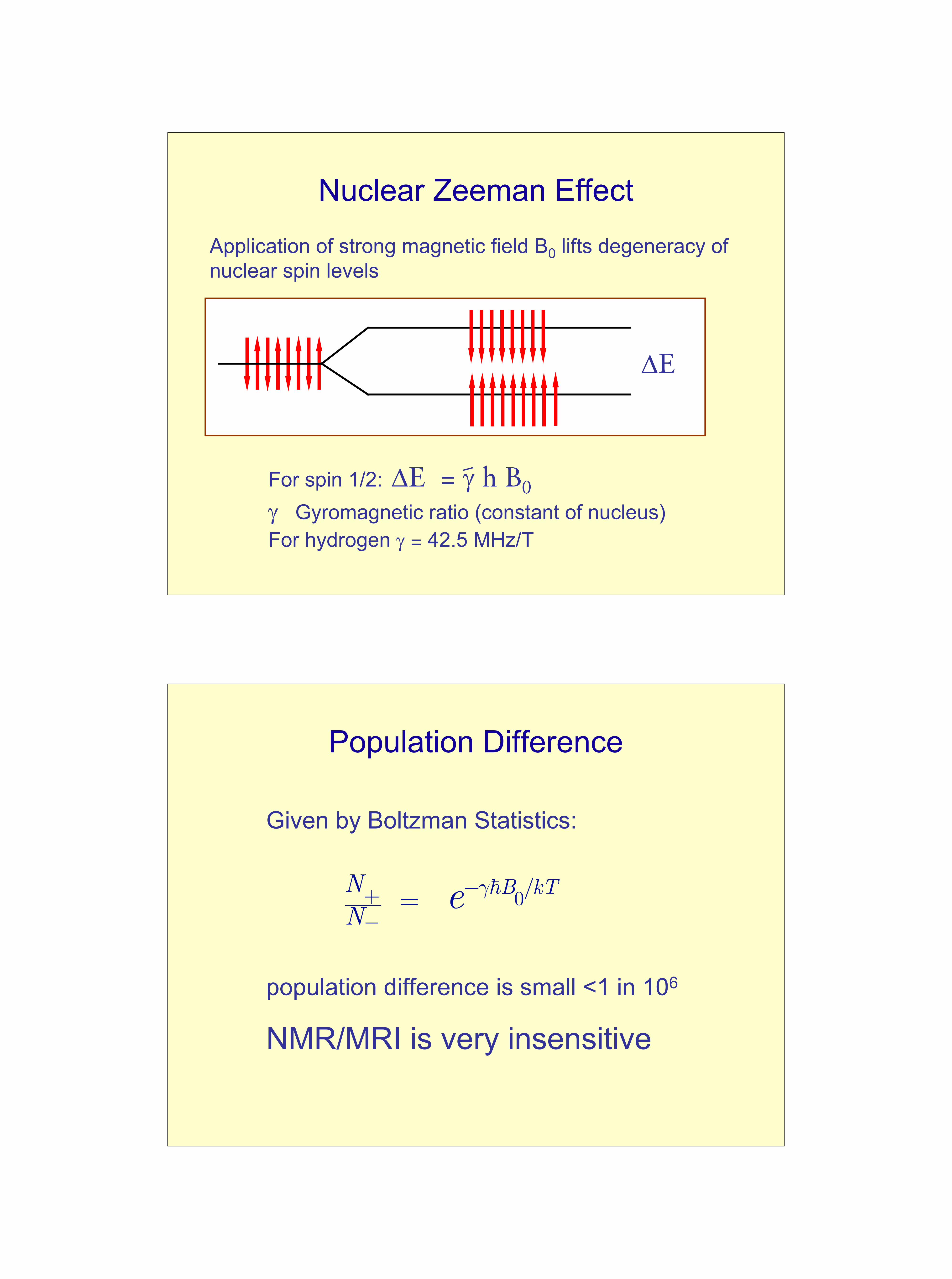
Nuclear Zeeman Effect

Application of strong magnetic field B0 lifts degeneracy of nuclear spin levels

For spin 1/2: ΔE = γ h B0γ Gyromagnetic ratio (constant of nucleus)For hydrogen γ = 42.5 MHz/T

ΔE

Population Difference

Given by Boltzman Statistics:

population difference is small <1 in 106

NMR/MRI is very insensitive

0/B kTNN

γ−+−

=

Semi-Classical Model

Gyroscopic motion of magnetic moment about B0

B0Use classical mechanics, Larmor precession

ω0 = - γ B0

μ

Ensemble Average

USE Classical language for behaviour of net magnetization

Same results as quantum treatment.

Spin Precession is like a Gyroscope

Gravity plays the role of the magnetic field for gyroscope .

Gyroscope wants to fall but is prevented by conservation of angular momentum.

Similarly Quantumbar magnets precess

Effect of RF Pulse

A Radio Frequency pulse at the resonant frequency causes the magnetization vector to rotate away from the Z axis

A 90 degree RF pulse tips the magnetization vector into the x-y plane

ω = γBo

xy

z o

RF

Magnetization in the x-y plane radiates RF which is the signal we measure

M

Magnetic Nuclei

Bloch Equations

Describe evolution of transverse and longitudinal components of magnetization. T1 and T2 control exponential relaxation and dephasing. T1 and T2 are properties of the material

Bloch Equations

1 1

2

/

/, ,

)( ) ( 0)(

( ) ( 0)

t Tz z

t Tx y x y

M t M t e

M t M t e

−−

−

= =

= =

Free Induction Decay (FID)

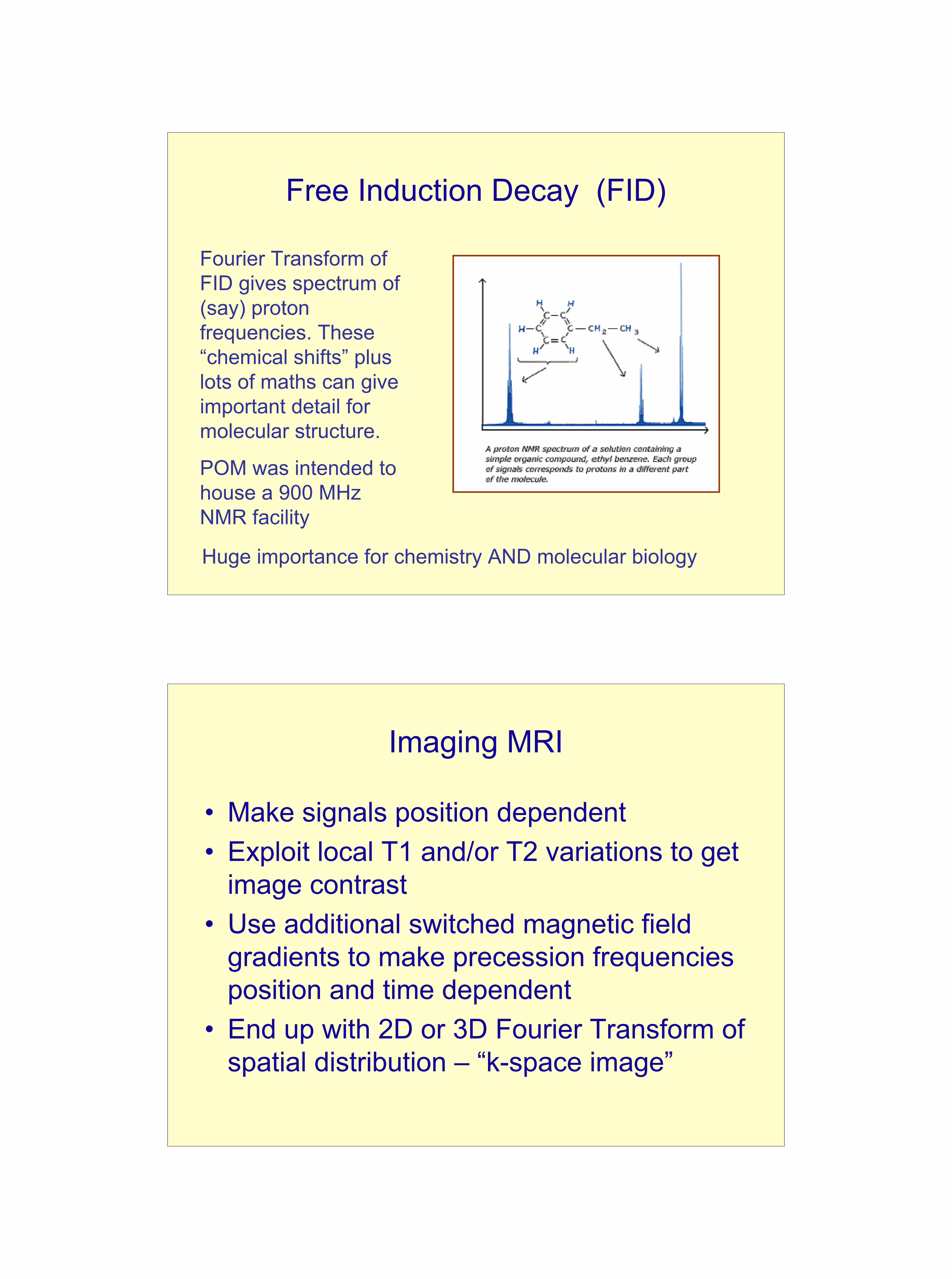
Free Induction Decay (FID)

Fourier Transform of FID gives spectrum of (say) proton frequencies. These “chemical shifts” plus lots of maths can give important detail for molecular structure.

POM was intended to house a 900 MHz NMR facility

Huge importance for chemistry AND molecular biology

Imaging MRI

• Make signals position dependent• Exploit local T1 and/or T2 variations to get

image contrast• Use additional switched magnetic field

gradients to make precession frequencies position and time dependent

• End up with 2D or 3D Fourier Transform of spatial distribution – “k-space image”

Gradients

Signal from sample in volume V at time t is:

where ρ is local spin density and φ is accumulated local phase offset:

Hence:

Gradients are driven to cover the whole of k-space over time and hence the FT of ρ.

0 ( , ) 3( ) ( )i t i t

VS t e e d rω φρ= ∫ rr

0 0( , ) ( )

t tx zyt G x G y G z dt dtφ = + + = ⋅∫ ∫r r G

03 where( ) ( )

ti

VdtS e d rρ ⋅ == ∫∫ k r k Gk r

Signal from sample in volume V at time t is:

where ρ is local spin density and φ is accumulated local phase offset:

Hence:

Gradients are driven to cover the whole of k-space over time and hence map out the FT of ρ.

0 ( , ) 3( ) ( )i t i t

VS t e e d rω φρ= ∫ rr

0 0( , ) ( )

t tx zyt G x G y G z dt dtφ = + + = ⋅∫ ∫r r G

03 where( ) ( )

ti

VdtS e d rρ ⋅ == ∫∫ k r k Gk r

From Games to Brains 20th February 2007 Richard Ansorge

Spin Echo


Pulse sequences Spin Echo


Pulse sequences Gradient Echo


Pulse sequences EPI

Very fast 10 ms/slice, used for fMRI, typically 128x128 voxels


Spectroscopy Possible

Big Voxel 5x5x5 cm

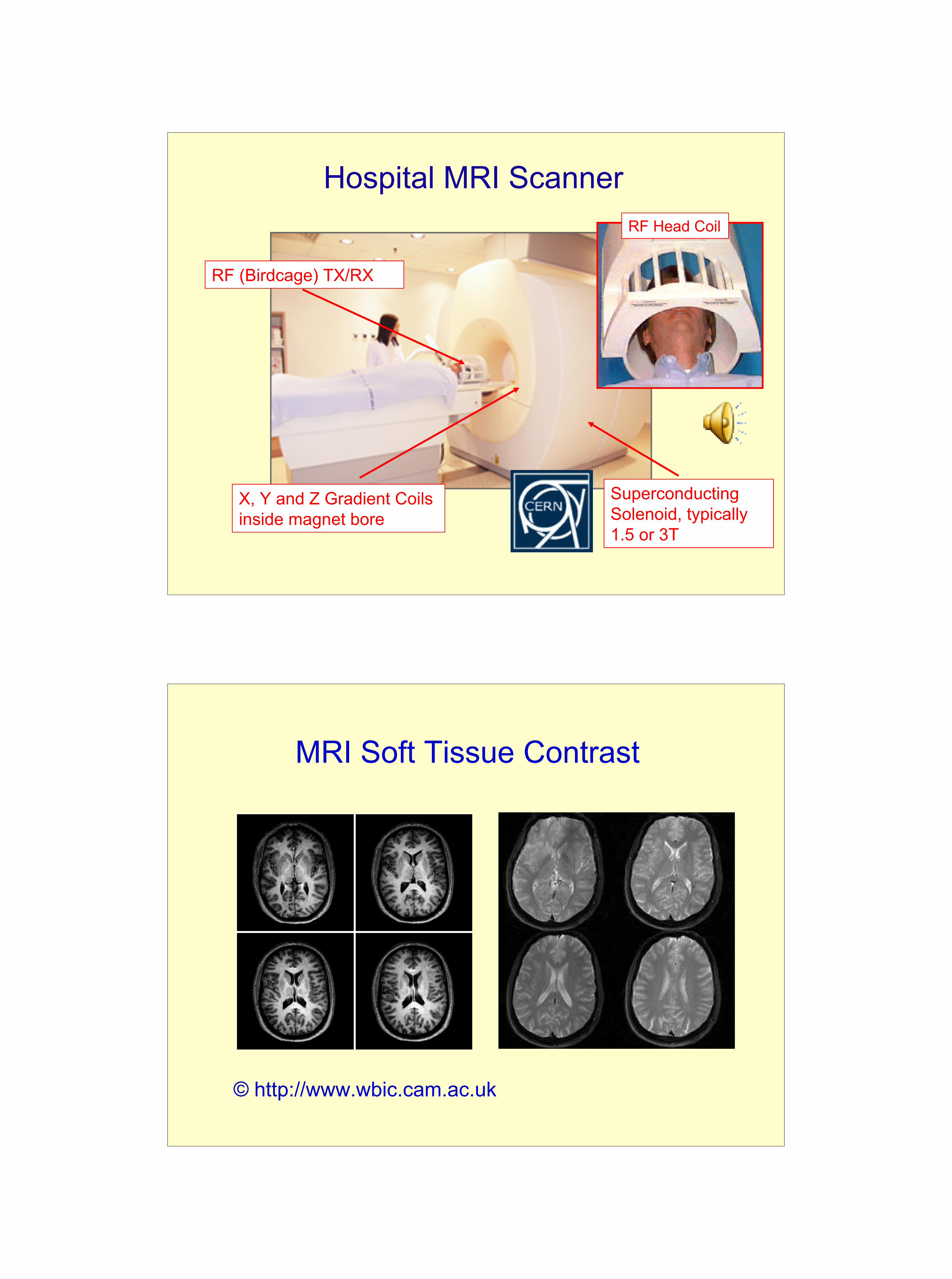
Hospital MRI Scanner

RF (Birdcage) TX/RX

X, Y and Z Gradient Coils inside magnet bore

Superconducting Solenoid, typically 1.5 or 3T

RF Head Coil

MRI Soft Tissue Contrast

© http://www.wbic.cam.ac.uk

3D Volume Data Sets

3D Volume Data Sets

Things to do with MRI

• Anatomy: proton density, T1, T2 etc• Flow – cardiac• Diffusion – trace neural pathways• Functional imaging

– research– surgical planning

• Interventional• Spectroscopy

Diffusion Imaging

Water diffuses more easily parallel to fibres

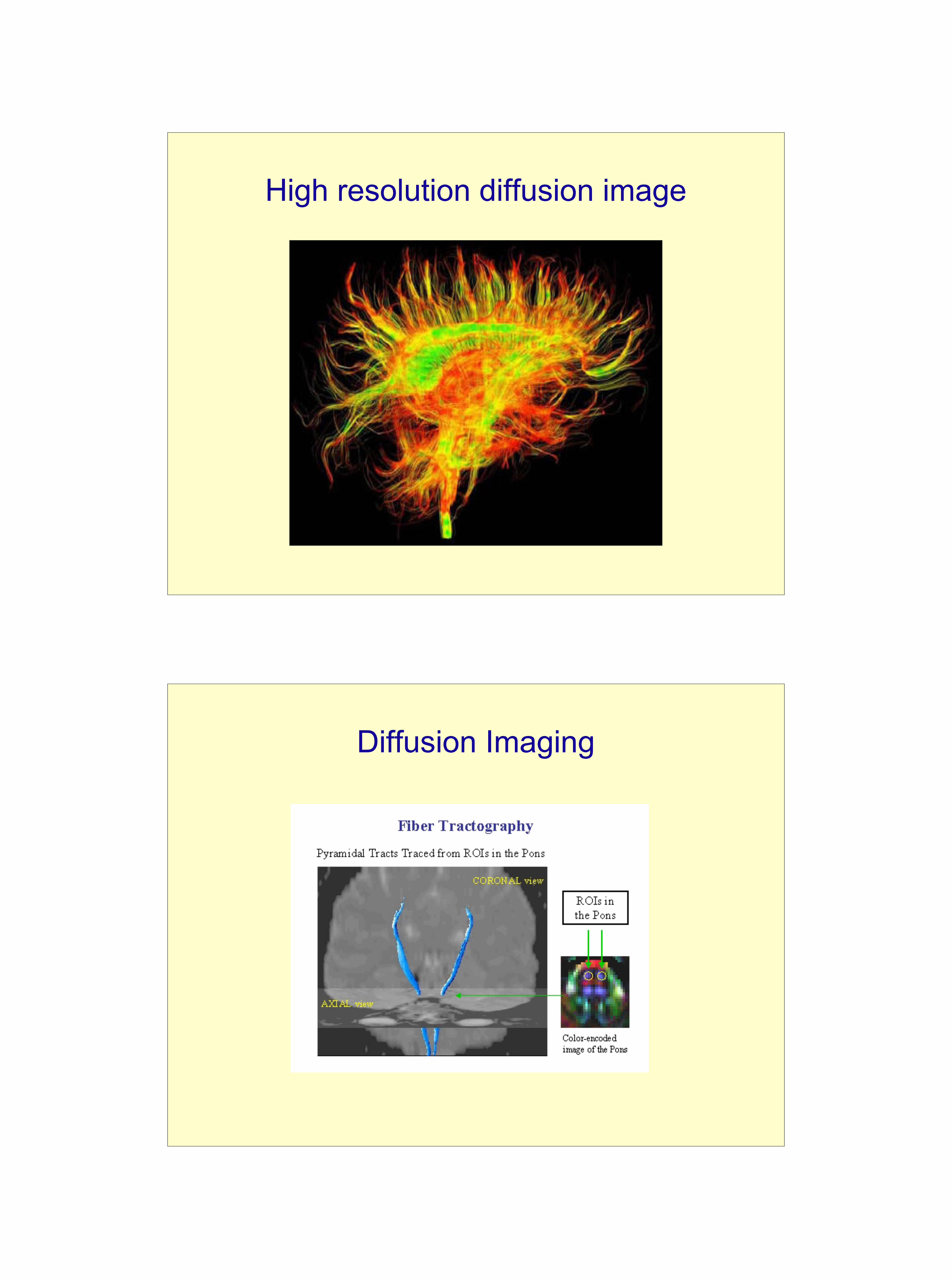
High resolution diffusion image

Diffusion Imaging

Muscle Fibres in Human Heart

Computed fits to Diffusion MRI of Human Heart

Functional MRI (fMRI)

• Monitor T2 or T2* contrast during cognitive task

• Acquire 20-30 slices every 4 seconds

• Design experiment to have alternating blocks of task and control condition

• Look for statistically significant signal intensity changes correlated with task blocks

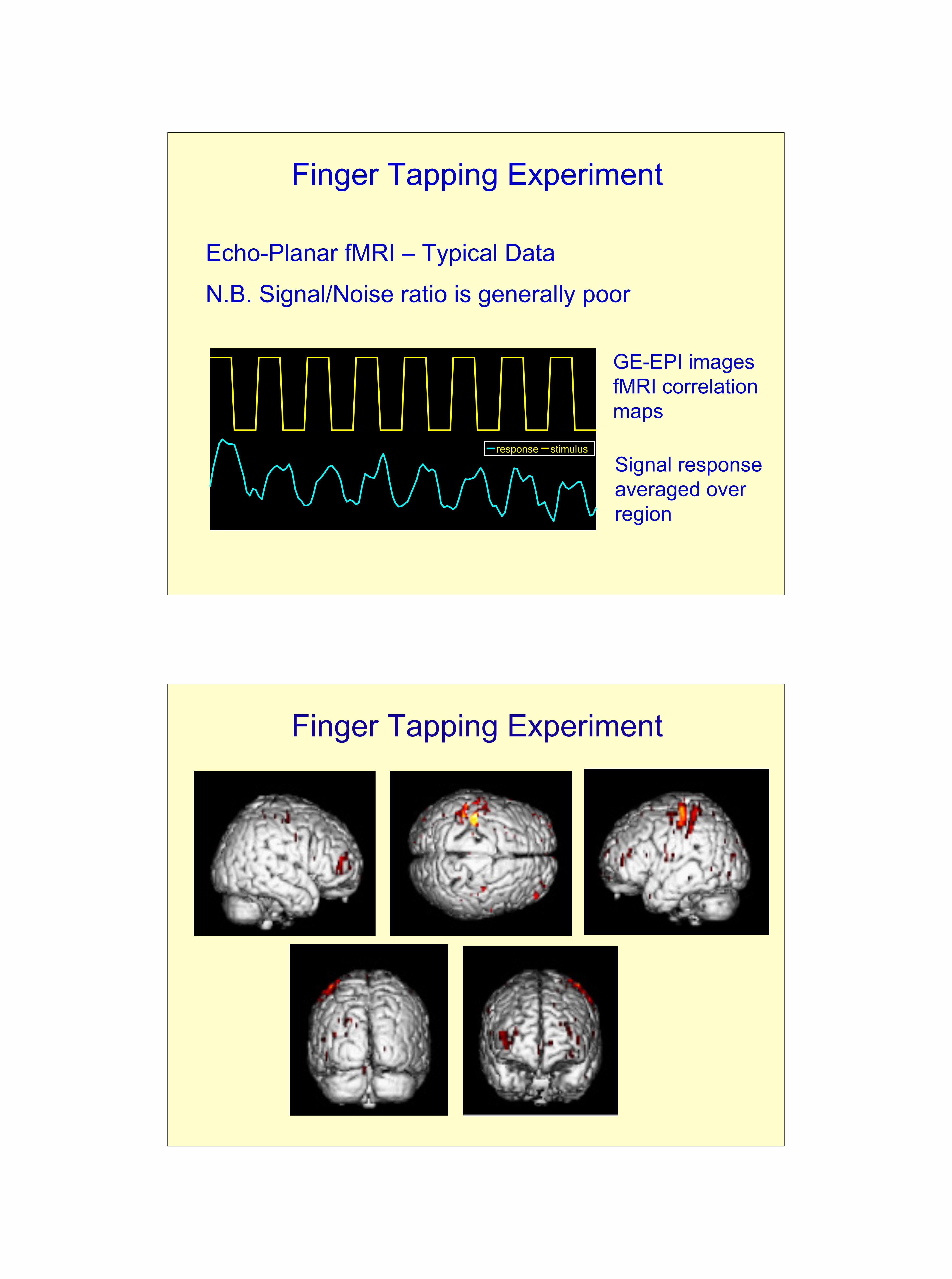
Finger Tapping Experiment

Echo-Planar fMRI – Typical Data

N.B. Signal/Noise ratio is generally poor

response stimulus

GE-EPI imagesfMRI correlation maps

Signal responseaveraged overregion

Finger Tapping Experiment

Segmentation

Can we sort out the anatomy?

Interventional MRI

This is still quite rare & expensive

Sensitivity

• 256 x 256 x 256 voxels typical• Can scale size of RF send/receive coils to

size of object.• Hence typical voxel dimension range is

0.050 mm to several mm.• BUT signal to noise depends on voxel

volume, will never do single cells.• Overnight acquisitions for mouse brains

Results from MRI: Iterative averages ~15 individuals

Typical Single Slice Affine Average, 15 subjects BS average, subdiv=2

BS average, subdiv=4 BS average, subdiv=7 Surface rendered average

Single slice note damage Iterative average, 14 subjects

As above after full BS registration to iterative average

Volume changes (Jacobian) from fitted BSplines

Richard Ansorge, IEEE HPMI October 2009

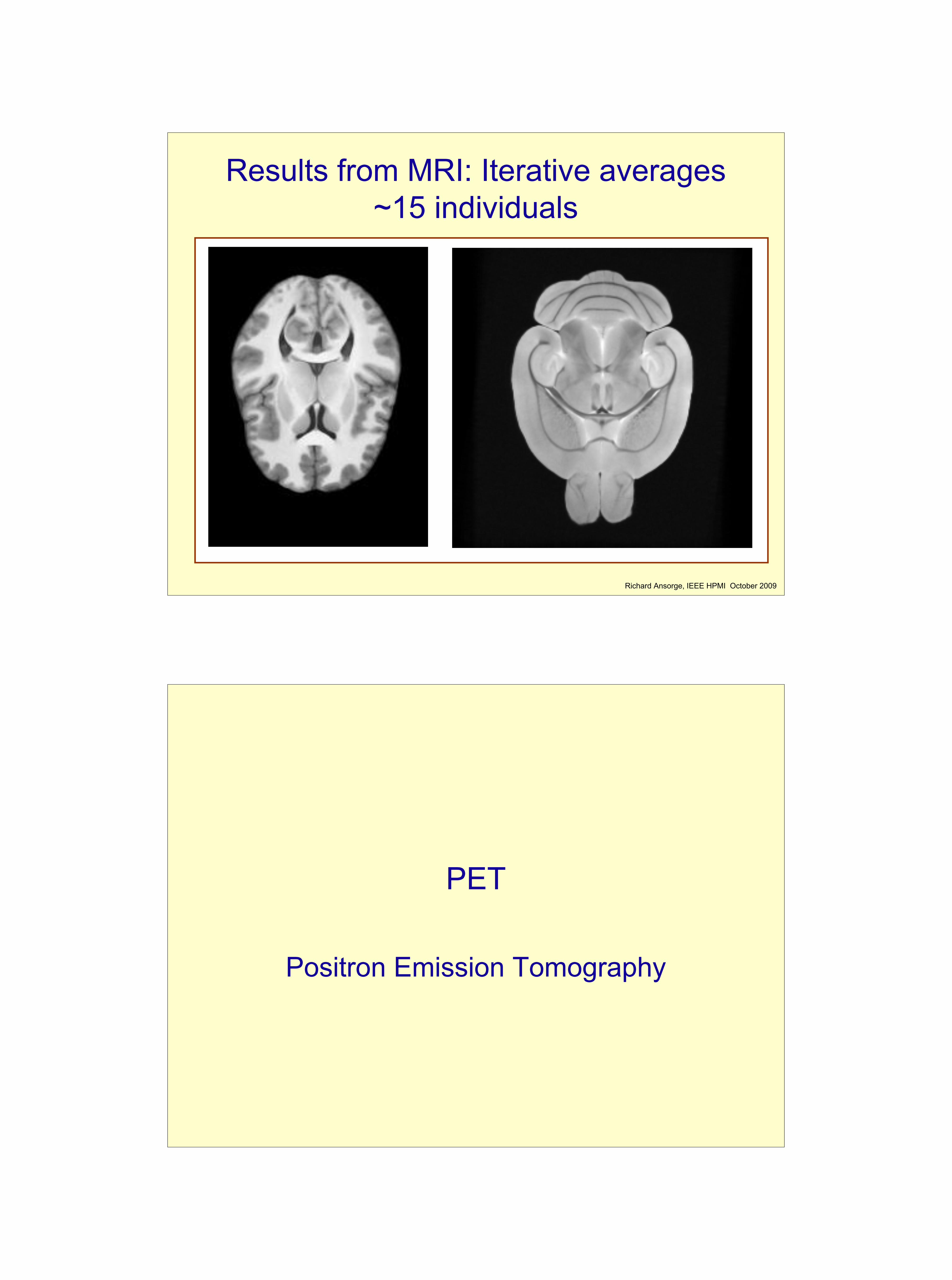
Results from MRI: Iterative averages ~15 individuals

Typical Single Slice Affine Average, 15 subjects

Richard Ansorge, IEEE HPMI October 2009

PET

Positron Emission Tomography

Positron Emission Tomography

• Origins in High Energy Physics (CERN).• Uses Positrons “anti-matter”.• Positrons annihilate with electrons to make

“pure energy”.• Actually makes 2 photons.

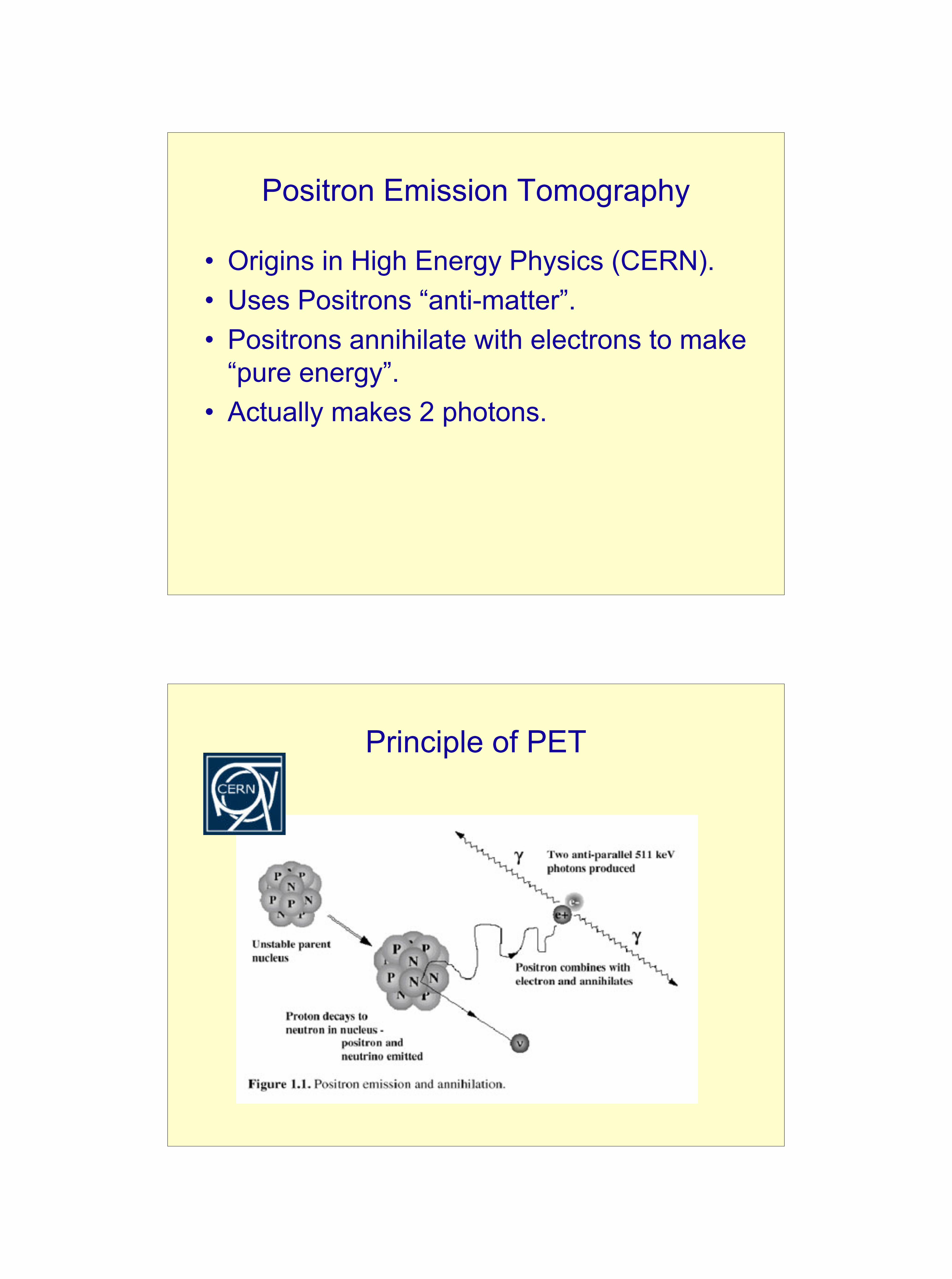
Principle of PET

Positron Emission Tomography (PET)

Inject (short-lived) positron emitting isotope.

Positron annihilates with electron giving pair of back to back 0.511 MeV gamma rays.

Detect both gammas using fast (5ns) coincidences, get “Line of Response” (LOR). Reconstruction of tracer distribution similar to CT.

18F 11C 13N 15O 68Ga

Maximum Energy (MeV) 0.63 0.96 1.20 1.74 1.90

Most Probable Energy (MeV) 0.20 0.33 0.43 0.70 0.78

Half-Life (mins) 110 20.4 9.96 2.07 68.3

Max Range in Water (mm) 2.4 5.0 5.4 8.2 9.1

Isotopes used in PET

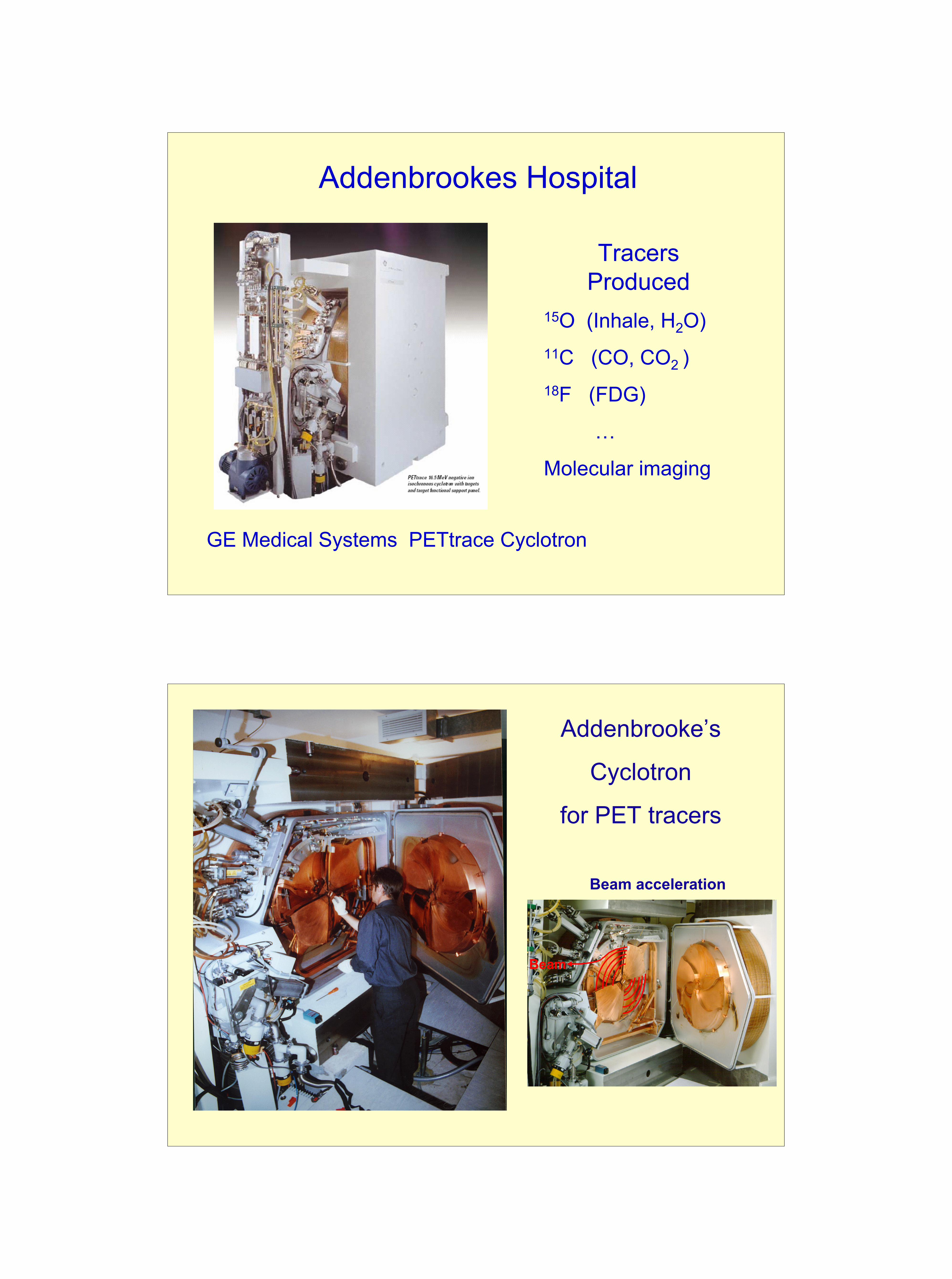
GE Medical Systems PETtrace Cyclotron

Tracers Produced

15O (Inhale, H2O)11C (CO, CO2 )18F (FDG)

…

Molecular imaging

Addenbrookes Hospital

Addenbrooke’s

Cyclotron

for PET tracers

Beam

Beam acceleration

PET is used to image the function of specific organs in the body not the anatomy.

PET is complimentary to the other imaging modalities.

PET is lower resolution but very sensitive.

FDG or Fluorodeoxyglucose

The single most important PET tracer.

FDG follows the same metabolic pathway as Glucose, i.e. it is “burnt” in actively metabolizing cells. THEN the 18F stays put. Thus 18F accumulates at “hot-spots” of high metabolic activity.

Whole Body PET

© http://www.cc.nih.gov/pet/images.html

F-18 fluorodeoxyglucose (FDG). Patient with colorectal cancer. Image is maximum intensity projection through attenuation corrected whole body image, acquired in multiple axial fields-of-view and reconstructed with OSEM algorithm. High uptake is seen in the kidney, liver, bladder, and tumor.

PET Visualization

New Tracer: Raclopride in Human Striatum

Wolfson Brain Imaging Centre &

MRC Cambridge Centre for Behavioural and Clinical Neuroscience

Combined PET & MRI

100 Gauss

5 Gauss

Shielding coil

Main coils

PET PMTs in low field region

PET Light guides

LSO Detectors

Cambridge PET-MR IPEM Sept 16 2009 Richard Ansorge

PET detector modules inserted in gap

PMT’s housed in magnetic screens and the signal wiring passing through the back plate of the external Faraday cage ( cover removed )

Axial FOV 7.6 cm Radial FOV 10 cm

LSO crystal blocks in 4 axial rings, 24 blocks per ring

Optical fibre 8x8 bundle

View up magnet bore Ring diameter 14.8 cm


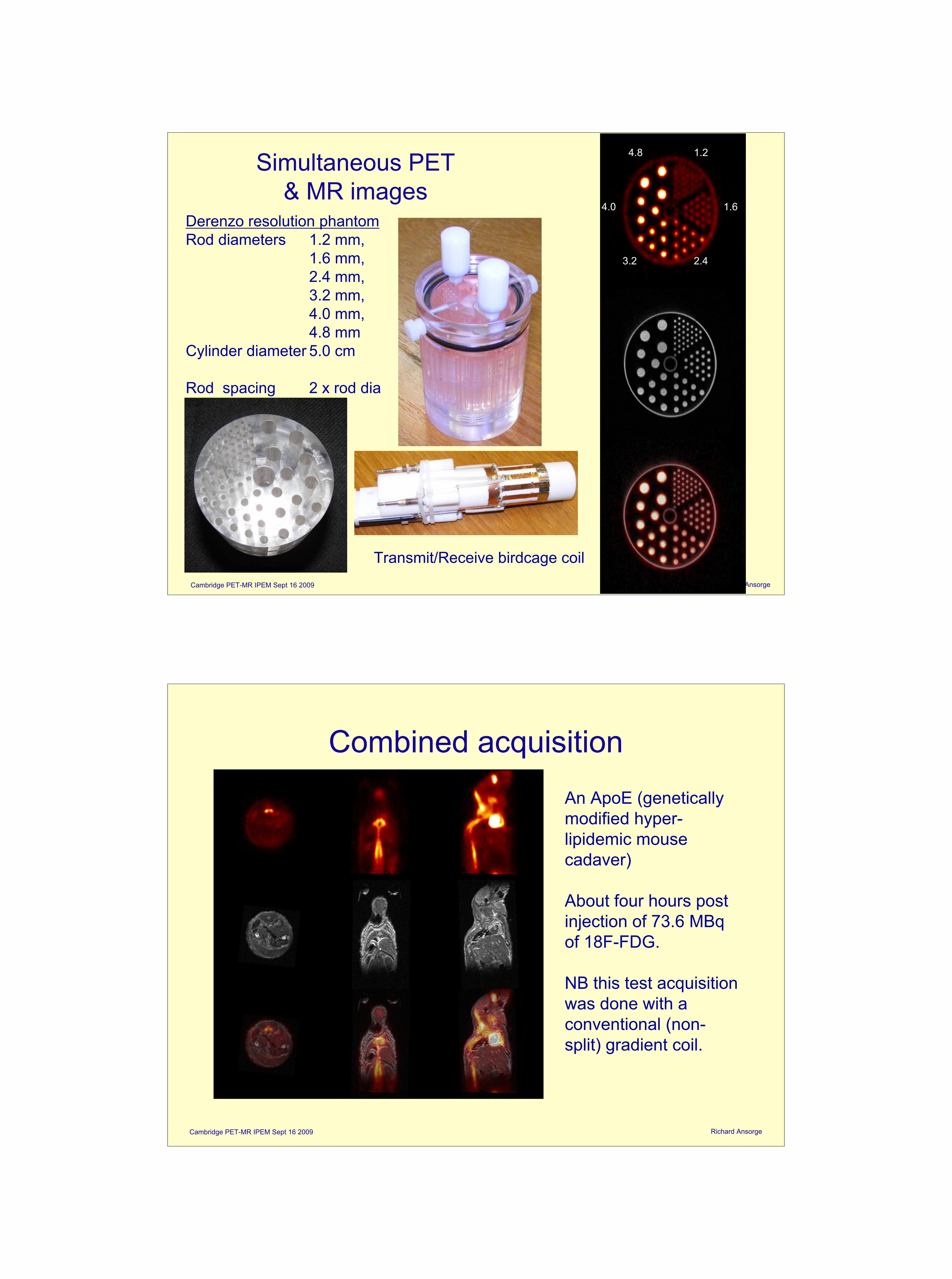
Simultaneous PET & MR images

Derenzo resolution phantomRod diameters 1.2 mm,

1.6 mm,2.4 mm,3.2 mm,4.0 mm,4.8 mm

Cylinder diameter 5.0 cm

Rod spacing 2 x rod dia

Transmit/Receive birdcage coil

4.8

4.0

1.2

2.4

1.6

3.2


Combined acquisition

An ApoE (genetically modified hyper-lipidemic mouse cadaver)

About four hours post injection of 73.6 MBq of 18F-FDG.

NB this test acquisition was done with a conventional (non-split) gradient coil.


Heart Images


System was moved to the new the Laboratory for Molecular Imaging in March 2008. Expected to be fully operational soon.

Imaging Suite Sept 2009: PET, MRI & PET-MR

Cambridge PET-MR IPEM Sept 16 2009Richard Ansorge


09/09/09 Quench Duct Finally Being Installed!

Questions?


multi core computing and mri -...

Documents