multi-camera calibration for 3dbos -...

17th International Symposium on Applications of Laser Techniques to Fluid Mechanics Lisbon, Portugal, 07-10 July, 2014

- 1 -

Multi-camera calibration for 3DBOS

Yves Le Sant1*, Violaine Todoroff2, Anthelme Bernard-Brunel3, Guy Le Besnerais3, Francis Micheli2, David Donjat2

1: Department of Experimental and Fundamental Aerodynamics, ONERA, Meudon, France

2: Department of Aerodynamics and Energetics Modeling, ONERA, Toulouse, France 3: Department of Modeling and Information Processing; ONERA, Palaiseau, France

* correspondent author: [email protected] Abstract Backgroung Oriented Schlieren (BOS) is a Schlieren-like method that can be used as a 3D quantitative method for measuring density in 3D flows. This can be done providing that there are enough points of view, at least 10, and that an accurate calibration of the multi-camera bench is available. We present here a study of multi-camera calibration for 3DBOS. We use a simple printed flat plate with a dotted regular pattern as calibration body (CB). The main issues are the workload, because there are several hundred of images, and the blurring effect. The blur affects the images of the CB when it is positioned in the common part of the fields of views of the cameras. Because of illumination limitation it can not be avoided. We present practical solutions and results for both issues. A GPU implementation allows to complete the calibration of a system with 12 cameras in less than 30mn. We also propose an uncertainty analysis using the jackknife. It is shown that the uncertainty of the estimation of the horizontal field of view (HFoV) is 0.04°. Moreover, HFoV is nearly identical for all cameras and quasi equal to the theoretical value. 1. Introduction Background Oriented Schlieren (BOS), is an experimental technique for measurement of the density field of a flow originally developed by Meier and Raffel (2000). It is based on measurement of the gradients of optical index which is then related to density via the Gladstone-Dale relationship. More precisely, the BOS experimental procedure consists in recording images of a textured background with a specific pattern in absence of a flow (reference frame) and with the flow in between the camera and the background. Image correlation algorithms such as the ones used in Particle Image Velocity (PIV) (Champagnat et al. 2011) provide the apparent displacement of the rays through the flow of interest. Knowing the calibration of the camera, one can deduce, from the displacements, the angle of deviation associated with the visualized flow. If one is able to measure the 3D deviation fields {εx, εy, εz} simultaneously from a sufficient number M of point of views, reconstruction of the instantaneous density fields can be achieved by numerical inversion of the following equation system:

( ) ( ) { }( )

MmJjIizyxudssu

Kmjimjirays

u ≤≤≤≤≤≤∈∂∂

= ∫∈

1,1,1,,,,,,,

ρε (1)

where K is a constant related to Gladstone-Dale equation. We use a paraxial approximation, hence integration is done along the 3D ray associated with each pixel (i,j) of each camera m where a deviation has been estimated. The first experimental demonstration of this instantaneous 3DBOS has been proposed by Atcheson et al. (2008), in the context of turbulent media rendering in computer graphics. A joint work between three departments of ONERA has been conducted to develop and validate a quantitative instantaneous 3DBOS method, using state of the art numerical methods for regularized inversion of (1) and a dedicated experimental bench developed at ONERA/DMAE in Toulouse to collect deviation fields associated to various flows. Numerical aspects of the methods and reconstruction results are the subject of a companion paper Todoroff et al (2014). Here we focus on the multi-camera calibration problem. The multi-camera calibration process aims at determining the equations of the 3D rays associated to each pixel of each image in a unique reference coordinate frame fixed to the workspace, which is located in the common part of the cameras field of view (Figure 1, left). Precise knowledge of these rays is of course required to write Eq. (1). There are several publications and available softwares for camera calibration (Zhang 2000, Bouguet 2002, DLR CalLab 2006) and most of them allow to deal with multi-camera


- 2 -

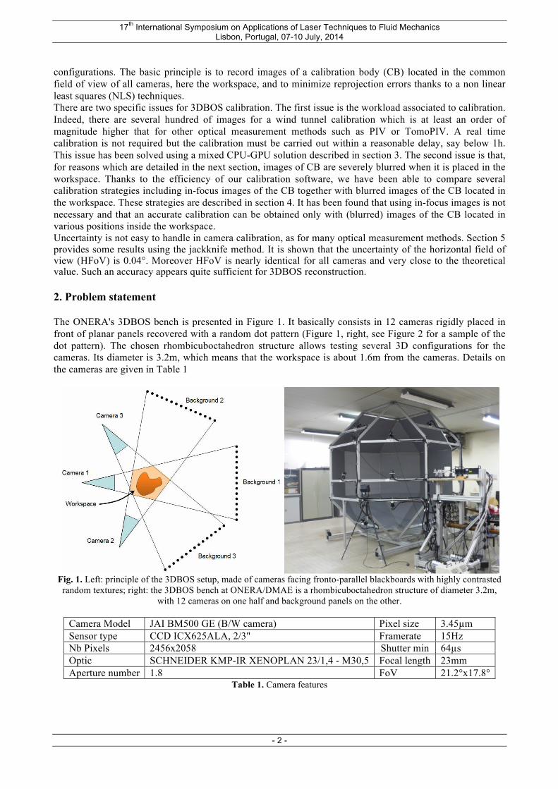
configurations. The basic principle is to record images of a calibration body (CB) located in the common field of view of all cameras, here the workspace, and to minimize reprojection errors thanks to a non linear least squares (NLS) techniques. There are two specific issues for 3DBOS calibration. The first issue is the workload associated to calibration. Indeed, there are several hundred of images for a wind tunnel calibration which is at least an order of magnitude higher that for other optical measurement methods such as PIV or TomoPIV. A real time calibration is not required but the calibration must be carried out within a reasonable delay, say below 1h. This issue has been solved using a mixed CPU-GPU solution described in section 3. The second issue is that, for reasons which are detailed in the next section, images of CB are severely blurred when it is placed in the workspace. Thanks to the efficiency of our calibration software, we have been able to compare several calibration strategies including in-focus images of the CB together with blurred images of the CB located in the workspace. These strategies are described in section 4. It has been found that using in-focus images is not necessary and that an accurate calibration can be obtained only with (blurred) images of the CB located in various positions inside the workspace. Uncertainty is not easy to handle in camera calibration, as for many optical measurement methods. Section 5 provides some results using the jackknife method. It is shown that the uncertainty of the horizontal field of view (HFoV) is 0.04°. Moreover HFoV is nearly identical for all cameras and very close to the theoretical value. Such an accuracy appears quite sufficient for 3DBOS reconstruction. 2. Problem statement The ONERA's 3DBOS bench is presented in Figure 1. It basically consists in 12 cameras rigidly placed in front of planar panels recovered with a random dot pattern (Figure 1, right, see Figure 2 for a sample of the dot pattern). The chosen rhombicuboctahedron structure allows testing several 3D configurations for the cameras. Its diameter is 3.2m, which means that the workspace is about 1.6m from the cameras. Details on the cameras are given in Table 1

Fig. 1. Left: principle of the 3DBOS setup, made of cameras facing fronto-parallel blackboards with highly contrasted random textures; right: the 3DBOS bench at ONERA/DMAE is a rhombicuboctahedron structure of diameter 3.2m,

with 12 cameras on one half and background panels on the other.

Camera Model JAI BM500 GE (B/W camera) Pixel size 3.45µm Sensor type CCD ICX625ALA, 2/3" Framerate 15Hz Nb Pixels 2456x2058 Shutter min 64µs Optic SCHNEIDER KMP-IR XENOPLAN 23/1,4 - M30,5 Focal length 23mm Aperture number 1.8 FoV 21.2°x17.8°

Table 1. Camera features


- 3 -

A well-known problem in multi-camera calibration is that it is often difficult to ensure that the calibration pattern is visible by all cameras. Many works propose non-planar calibration bodies in order to maximize simultaneous visibility, an extreme example being the point calibration proposed by Svoboda et al. (2005). In the 3DBOS configurations studied here, cameras are positioned in a half space, the other being occupied by the backgrounds. Hence a planar calibration pattern placed in the workspace is always visible by at least 3 cameras. It is sufficient to enforce consistency of the calibration over all camera parameters. However, in the BOS multi-camera setting, each camera is adjusted so that the background image is sharp, in order to maximize the performance of image correlation and obtain accurate displacement measurements. As a consequence, the workspace is out of focus as shown in Figure 2.

Fig. 2 An image with CB located in the workspace. CB is a paper sheet stuck on a Plexiglas plate using the electrostatic effect. The detail on the right shows that the background is in focus (upper part of the image)

while the workspace is not.

Indeed, it is not possible to reduce the aperture of the camera so as to have a sufficient depth of field that includes the workspace. Reducing the aperture reduces the incoming light and leads to a difficult problem of illumination, considering the large volume at hand (let us recall that the diameter of the structure in Figure 1 is 3.2m). Hence we are forced to work with large apertures and to consider a multi-camera calibration problem where the common field of view is severely blurred. Figure 3 presents blur measurements made using a knife-edge method. The estimation is done by imaging a tilted edge pattern at various distances from the camera (Fig. 3, up-left). Intensities measured along a line of this image provide a sampling of the profile of the edge. After registration, these intensities collected over several lines lead to a subpixel irregular sampling of the profile, which is fitted by an integrated Gaussian model (Fig. 3, up-right). The blur size is is then estimated by the standard deviation of the Gaussian function obtained by deriving the fitted curve (in the case of Fig. 3, upper line, this standard deviation is 5.5 pixels). The curve on the bottom part of Figure 3 presents estimated blur sizes for various positions of the edge pattern in front of one of the 12 cameras. Two regions have been explored: close to the in-focus plane, ie. around 3.2m, where the background used for BOS is positioned (red crosses), and halfway, around 1.5m, in the workspace (blue crosses). In the workspace, the blur size is quite high, between 8 and 10 pixels.


- 4 -

Fig. 3 Estimation of the blur size for one camera of the 3DBOS bench by the knife-edge method. Up-left: a blurred

image of a tilted edge. Up-right: sampling of the edge profile provided by the intensities measured on the image on the left and result of a Gaussian fit (red line). Bottom: estimated blur size (in pixels) vs. distance from the edge pattern to

the camera (in cm). The dot pattern, even blurred as in Figure 2, can still be used for calibration since the dot detector we use for regular calibrations is moderately sensitive to blurring. Anyway, blurring has certainly an effect on the accuracy of calibration: this is discussed in following sections.

3. The multi-camera calibration pipeline Camera calibration is required for nearly all of optical methods used in wind tunnel testing as PSP (Pressure Sensitive Paint, Liu and Sullivan 2005), MDM (Model Measurement Method, Le Sant et al. 2007) PIV and TomoPIV. It follows the general flowchart presented in Figure 4. The CB can be as simple as a flat dotted plate or a two levels plate as it is usual for stereoscopic PIV. With a simple flat CB, several images are taken thus leading to a calibration with a few dozen of images for the most demanding method which is TomoPIV. The computation time is then not an issue while it is one for 3DBOS because there are much more images. Trying to obtain a reasonable total computation time implies to optimize each step of the flow chart shown in Figure 4. The computation are done on a usual laptop (Intel Core i7-2630QM @ 2.00GHz) equipped with a NVIDIA GTX580M GPU board (2Gb, 384 CUDA cores).


- 5 -

Fig. 4 Flow chart of camera calibration

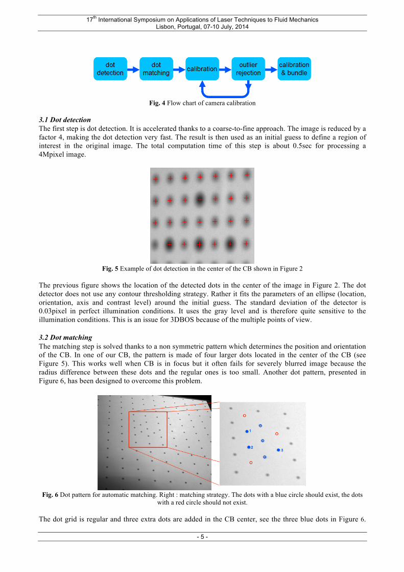
3.1 Dot detection The first step is dot detection. It is accelerated thanks to a coarse-to-fine approach. The image is reduced by a factor 4, making the dot detection very fast. The result is then used as an initial guess to define a region of interest in the original image. The total computation time of this step is about 0.5sec for processing a 4Mpixel image.

Fig. 5 Example of dot detection in the center of the CB shown in Figure 2

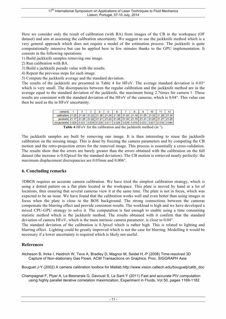
The previous figure shows the location of the detected dots in the center of the image in Figure 2. The dot detector does not use any contour thresholding strategy. Rather it fits the parameters of an ellipse (location, orientation, axis and contrast level) around the initial guess. The standard deviation of the detector is 0.03pixel in perfect illumination conditions. It uses the gray level and is therefore quite sensitive to the illumination conditions. This is an issue for 3DBOS because of the multiple points of view. 3.2 Dot matching The matching step is solved thanks to a non symmetric pattern which determines the position and orientation of the CB. In one of our CB, the pattern is made of four larger dots located in the center of the CB (see Figure 5). This works well when CB is in focus but it often fails for severely blurred image because the radius difference between these dots and the regular ones is too small. Another dot pattern, presented in Figure 6, has been designed to overcome this problem.

Fig. 6 Dot pattern for automatic matching. Right : matching strategy. The dots with a blue circle should exist, the dots

with a red circle should not exist. The dot grid is regular and three extra dots are added in the CB center, see the three blue dots in Figure 6.


- 6 -

The matching strategy is simple: select randomly three dots and assume they are the three extra dots. This creates an image metric used to check if other dots exist at the computed location (the blue ones) and if other dots does not exist (the red one). There is only one valid solution so the strategy is to check all the solutions and to select the one that passes the validation test. Thanks to parallel programming on GPU, the computation time of this test is negligible (just a few ms) compared to the reading/saving data overhead. The outputs of the dot matching step are the matched dots and an initial guess of the camera location which is assessed using the matched dots. 3.3 Calibration The calibration step takes place when the matching phase is completed. The parameters are gathered into three groups:

• The intrinsic group containing 7 parameters for each camera which describes the sensor and lens properties: the field of view (FoV), the radial distortions parameters (K1,K2), the tangential distortion parameters (P1, P2) and the location of the principal point (Co,Lo that are the coordinates of the intersection of the lens axis with the sensor);

• The extrinsic group defines the position and orientation of the camera in the world coordinate system. There are 6 parameters that are 3 angles and 3 distances.

• CB motion parameters: as the CB is moved to increase the number of images, the CB motions have to be included in the sought parameters. The world coordinate system is fixed to the first CB position called the CB reference. For the other ones, there are 6 motion parameters (3 rotations and 3 translations).

Calibration is a nonlinear least squares (NLS) problem that we solve using the Levenberg-Marquardt method (LM). The dot matching step provides a quite accurate assessment of the extrinsic group and of the CB motion parameters. The initial guess is for FoV its theoretical value (21.2°, see Table 1) and 0 for the other intrinsic parameters. Let us assume there are 10 cameras, 100 dots on the CB and 100 CB motions (thus there are 10x(100+1)=1010 images). There are 130 camera parameters and 600 CB motion parameters; the total is then 730 parameters. When the parameters are fixed, one can computes the image projection of the dots using the grid in Figure 7 where each square represents the dot projections (DP) for one camera and one CB location. There are 1000 DP for each CB location, 10 100 DP for each camera and the grand total is 101 000 DP. The computations are done in a massively parallel approach thanks to a GPU.

Fig. 7. Computing Grid.

The LM method computes the pseudo-Hessian matrix H. Each element is the sum over the whole calibration set of the cross product of the first derivatives:

j

dcm

Mm Cc Dd i

dcmji p

PpP

H∂

∂

∂

∂= ∑ ∑ ∑

= = =

,,

,1 ,1 ,1

,,, (2)

where M is the number of CB motions, C is the number of cameras, D is the number of dots on the CB, pi and pj are the parameters i and j, P is the projection function used to compute DPs. The first derivatives are computed numerically on the GPU. The implementation assesses at the same time the first derivatives for all parameters of the same type. Thus there are 7(intrinsic) + 6(extrinsic) + 6(CB motion)=19 computations. This enables to increase the GPU workload which is the best way to use its full


- 7 -

capacities. Most of the computations are done on the GPU but matrix inversion and other subtasks as updating camera parameters. The duration of the computation is about 1mn for the heavier test (about 12 cameras, 120 CB motions) which is small compare to the first steps: 10mn for dot detection and 3mn for dot matching.

3.4 Outlier rejection The next step after calibration is outlier rejection. They are usually badly illuminated dots ore damaged dots as the one shown in Figure 13 (the gray spot at the lowest position does not appear symmetric as it should be).

Fig.8 Outlier rejection

The rejection is done automatically removing dots having a projection error greater than three times the standard deviation computed on the relevant image. There are just a few outliers for a regular calibration, typically less than 0.1% of the detected dots. The calibration is again carried out after dot rejection and the process is repeated until a stable calibration is obtained. Usually only one rejection step is needed. 3.5 Bundle adjustment (BA) The last step is to calibrate also the calibration body, which is called bundle adjustment (BA). The calibration body is stiff enough but its exact shape is not known. It could be measured with a 3D measuring system but this would be expensive and it would slow down the calibration process. We have chosen to calibrate it together with camera calibration since a lot of images are available. Bundle adjustment (BA) is just a matter of adding extra parameters that are the 3D dot locations. If there are 100 dots, this adds 300 parameters. This is not too much compared to the usual ≈1000 camera and CB motion parameters. However this method increases significantly the workload since each dot location is coupled with all cameras and all CB motions. We have developed a so-called pseudo-bundle adjustment method considering BA as a sub-problem. The 3D dot locations are computed at each iteration of the LM method using the estimated camera and CB motion parameters. This computation is done on the GPU at nearly no cost and thus does not slow down the calibration. A rigorous manner would be to compute the 3D locations even when computing the first derivatives. However there are so many camera and CB motion parameters that modifying only one of them has nearly no impact on the 3D dot locations. The more there are cameras and CB motions, the more valid is the pseudo BA method. The pseudo-BA method has been validated using simulations. Typical 3DBOS calibrations without noise were simulated. The CB shape was then slightly modified which created dot projection errors. Calibration with BA was carried out and all the parameters as well as the theoretical CB shape were retrieved exactly. The whole calibration is carried out within 30mn and just a few minutes are consumed by the calibration itself. It should be noted that the convergence of the calibration is fast since a stable result is obtained after 20 iterations. This is less than with regular SPIV calibration which is likely due to the strong connection between the cameras.

4. Calibration and the effect of blur on accuracy


- 8 -

As already discussed, the calibration body must be placed in the workspace so that the cameras are calibrated in a common world coordinate system. This enables to determine the extrinsic parameters of all cameras. However, has shown in Figure 2, CB is out of focus: the images are blurred. In the following, the set of images of the CB in the workspace is called the 'OF' (Out of Focus) dataset: it has been made with 27 CB motions leading to (27+1)x12=336 images. The calibration process described in Section 3 has been run on the OF dataset: some results are presented in Table 2below.

Table 2. Calibration using the OF dataset. Up: reprojection error. Down: estimation of the HFoV for each camera (°). The calibration is carried out with and without BA. Both options provide an HFoV nearly constant over all cameras. The average value is very close to the theoretical one (21.2°, see Table 1). Nevertheless the standard deviation with BA is 0.043° is half the value obtained without BA (0.084°). The consistency between the cameras is then better with BA than without BA. This demonstrates the interest in using BA together with the reprojection error decrease. However, the reprojection errors are quite high compared to the theoretical accuracy of the dot detector (0.06pixel). The reprojection errors for a typical image are presented in Figure 14. The image on the left hand side shows the errors without BA. Their smooth variations indicate that they are dominated by a systematic error on the CB geometry, which motivates the use of BA. On the right part, with BA, the error vectors are smaller and look randomly oriented, which means they derive from dot detection errors which are related to the blur.

Fig. 9 Left: errors without BA (max arrow length=1.08pixel). Right : errors with BA (max arrow length=0.68pixel)

To gain knowledge on the impact of blur in the calibration process, we have also recorded several in focus images of the CB. This second image calibration set is called 'IF' (In Focus) set. The images are obtained with the CB placed close to the BOS background, see Figure 10.


- 9 -

Fig.10 An image of the calibration body placed close to the background (IF=in focus). The detail on the right shows

that both the background panel and the CB are in focus.

CB looks in the previous image twice smaller than in Figure 2 because it is at 3.2m from the camera instead of 1.6m. As a consequence, more CB motions are needed to ensure that the whole camera field of view is covered. We use 30 images for each camera, an example is shown in Figure 10.

Fig. 11 Dot locations obtained with 30 CB motions in the IF dataset

Note that these images allow to calibrate only the intrinsic parameters for each camera. Indeed the extrinsic parameters cannot be identified because CB is not in the common field of view. However, one can use the whole dataset for identifying the shape of the CB. Indeed, letting apart the global position of the CB, the 3D location of the dots with respect to a reference one, are observed by each camera. They are common parameters that can be estimated by a simple modification of the BA process. The results of the IF calibration are presented below. Table 3presents the reprojection error and the estimated HFoV for each camera. As expected, the reprojection error with BA is much smaller than with the blurred images of the OF dataset, with a standard deviation of 0.06pixel which is only twice the theoretical accuracy of the dot detector. The HFoV are consistent with the OF estimation, except for camera 10. This is probably due to the fact that the CB motions were not sufficient to cover the camera field of view. This is clearly a practical issue with this process: each camera field of view has to be carefully covered, which means a large number of images. In contrast, the OF estimation benefits from the fact that the CB is viewed by more than one camera, at each position in the workspace. It is more efficient in terms of CB manipulations, and it also improves the consistency of the estimation. Indeed, without camera 10 the standard deviation of IF estimation is still 0.15°, which is 3.5 times the standard deviation obtained using the OF dataset.

Table 3. Calibration using the IF dataset. Up: reprojection error. Down: estimation of the HFoV for each camera.


- 10 -

The HFoV without BA exhibits large errors (with respect to the theoretical value of 21.2°) and high standard deviation (0.92°). This demonstrate that BA is required for the IF set while it improves only moderately the calibration for the OF set. This highlights that the connection between the cameras for the OF set is a big advantage. It is also interesting to compare CB shape estimations provided by the BA using the OF or the IF dataset. Figure 11 shows the 3D shape of the calibration body using IF, with a magnification x50 of the deformation in the direction normal to the main plane. It shows a bending of about 0.15mm which is rather small compared to the size of the CB which is 400x280mm. The shape obtained with the OF dataset is globally very similar to the one shown in Figure 11.

Fig.12 The shape of the calibration body obtained with BA using the IF dataset.

The deformation in the direction normal to the main plane is magnified x50. Figure 12 compares the in-plane vectors of correction between the ideal CB (planar with perfectly regular grid) and the estimated CB with the IF (left part) and the OF (right part) dataset. At first sight, the two vector fields are similar. However corrections provided by BA on the OF datasets are more irregular. Note also that significant corrections are estimated for the four large dots at the CB center in the OF set. These irregularities are certainly due to the effect of blur on the dot localization, which is likely to be higher for larger dots. Hence, at least a part of the detection error related to blur has been transferred to the 3D dots location error by the BA. As a result, these errors do not pollute the estimation of extrinsic and intrinsic parameters, which could explain the good performance of HFoV estimation from OF dataset. A rough estimate of this part is 0.2pixel/0.035mm, which is obtained comparing the four large dots to their neighbouring dots.

Fig.13 In plane corrections provided by the BA with the IF (left) and the OF (right) datasets. The correction for the

largest arrows is 0.4mm (CB size= 400x280mm) As a conclusion, calibration with blurred images of the CB positioned in the workspace requires BA and leads to quite accurate extrinsic/intrinsic parameters. While reprojection errors are higher than usually encountered with in-focus images, it is suspected that most of these errors are related to the higher variance of dot localization and are transferred to the CB shape estimation in the BA process.

5. Uncertainty assessment


- 11 -

Here we consider only the result of calibration (with BA) from images of the CB in the workspace (OF dataset) and aim at assessing the calibration uncertainty. We suggest to use the jackknife method which is a very general approach which does not require a model of the estimation process. The jackknife is quite computationally intensive but can be applied here in few minutes thanks to the GPU implementation. It consists in the following operations: 1) Build jackknife samples removing one image. 2) Run calibration with BA. 3) Build a jackknife pseudo value with the results. 4) Repeat the previous steps for each image. 5) Compute the jackknife average and the standard deviation. The results of the jackknife are presented in Table 4 for HFoV. The average standard deviation is 0.03° which is very small. The discrepancies between the regular calibration and the jackknife method are in the average equal to the standard deviation of the jackknife, the maximum being 2.7times for camera 1. These results are consistent with the standard deviation of the HFoV of the cameras, which is 0.04°. This value can then be used as the in HFoV uncertainty.

Table 4 HFoV for the calibration and the jackknife method (in °).

The jackknife samples are built by removing one image. It is then interesting to reuse the jackknife calibration on the missing image. This is done by freezing the camera parameters and by computing the CB motion and the retro-projection errors for the removed image. This process is essentially a cross-validation. The results show that the errors are barely greater than the errors obtained with the calibration on the full dataset (the increase is 0.02pixel for the standard deviation). The CB motion is retrieved nearly perfectly: the maximum displacement discrepancies are 0.03mm and 0.006°. 6. Concluding remarks 3DBOS requires an accurate camera calibration. We have tried the simplest calibration strategy, which is using a dotted pattern on a flat plate located in the workspace. This plate is moved by hand at a lot of locations, thus ensuring that several cameras view it at the same time. The plate is not in focus, which was expected to be an issue. We have found that the calibration works well and even better than using images in focus when the plate is close to the BOS background. The strong connections between the cameras compensate the blurring effect and provide consistent results. The workload is high and we have developed a mixed CPU-GPU strategy to solve it. The computation is fast enough to enable using a time consuming statistic method which is the jackknife method. The results obtained with it confirm that the standard deviation of camera HFoV, which is the main intrinsic camera parameter, is close to 0.04°. The standard deviation of the calibration is 0.3pixel which is rather high. This is related to lighting and blurring effect. Lighting could be greatly improved which is not the case for blurring. Modelling it would be necessary if a lower uncertainty is required which is likely not useful. References Atcheson B, Ihrke I, Heidrich W, Tevs A, Bradley D, Magnor M, Seidel H.-P (2008) Time-resolved 3D

Capture of Non-stationary Gas Flows. ACM Transactions on Graphics, Proc. SIGGRAPH Asia Bouguet J-Y (2002) A camera calibration toolbox for Matlab.http://www.vision.caltech.edu/bouguetj/calib_doc Champagnat F, Plyer A, Le Besnerais G, Davoust S, Le Sant Y (2011) Fast and accurate PIV computation

using highly parallel iterative correlation maximization, Experiment in Fluids, Vol 50, pages 1169-1182


- 12 -

DLR Calibration Laboratory (DLR CalLab) (2006). http://www.dlr.de/rm/en/desktopdefault.aspx/tabid-3925/6084_read-9201/

Le Sant Y, Mignosi A, Touron G, Deléglise B (2007) Model deformation measurement (MDM) at onera 25th

AUAA Applied Aeridynamics Conference, Miami, FL. Liu T, Sullivan J.P (2005) Pressure and Temperature Sensitive Paints. Springer Raffel M, Richard H, Yu Y, Meier G (2000) Background oriented stereoscopic schlieren for full scale

helicopter vortex characterization, 9th Int. Symp. on flow visualization, Heriot-Watt Univ., Edinburgh, UK Todoroff V. et al. (2014) Reconstruction of instantaneous 3D flow density fields by a new direct regularized

3DBOS method. Int. Symp. on Applications of Laser Techniques to Fluid Mechanic, Lisbon Svoboda T,Martinec D, Pajdla, T (2005) A convenient multicamera self-calibration for virtual environments.

Presence: Teleoperators & virtual environments, 14(4), 407-422. cf. http://cmp.felk.cvut.cz/~svoboda/SelfCal/index.html

Zhang Z (2000) A Flexible New Technique for Camera Calibration. IEEE Transactions on Pattern

Analysis and Machine Intelligence, Volume 22:1330 – 1334

multi-camera calibration for 3dbos -...

Documents