Multi-armed Bandits underGeneral Depreciation and Commitment

Wesley CowanDepartment of Mathematics, Rutgers University110 Frelinghuysen Rd., Piscataway, NJ 08854

Michael N. KatehakisDepartment of Management Science and Information Systems

Rutgers Business School, Newark and New Brunswick100 Rockafeller Road, Piscataway, NJ 08854, USA

June 10, 2014

1

Abstract

Generally, the multi - armed bandit problem has been studied under the setting that at eachtime step over an infinite horizon a controller chooses to activate a single process or bandit outof a finite collection of independent processes (statistical experiments, populations, etc.) fora single period, receiving a reward that is a function of the activated process, and in doing soadvancing the chosen process. Classically, rewards are discounted by a constant factor β ∈(0,1) per round.

In this paper, we present a solution to the problem, with potentially non-Markovian, un-countable state space reward processes, under a framework in which, first, the discount factorsmay be non-uniform and vary over time, and second, the periods of activation of each banditmay be not be fixed or uniform, subject instead to a possibly stochastic duration of activationbefore a change to a different bandit is allowed. The solution is based on generalized restart-in-state indices, and it utilizes a view of the problem not as ‘decisions over state space’ but rather‘decisions over time’.

Keywords: Machine learning, Dynamic Data Driven Systems; Autonomous reasoning and learn-ing; Markovian decision processes; adaptive systems.

1 Introduction and Summary

Generally, the multi-armed bandit problem has been described in terms of sequentially allocatingeffort to one of N independent processes, or bandits, for instance sequentially assigning measure-ments to one of N possible statistical populations or measurements in clinical trials. In what follows,we discuss the problem in terms of bandit activation. In each period, a controller chooses a singlebandit to activate from the N available, basing that decision on all information available about allbandits at that time. The activated bandit yields a reward that depends on its current state, and thenmoves to a new state according to a probability law of motion that is a function of that bandit’shistory. Each bandit is taken to be independent of the others. Inactive bandits in a period yield norewards, and their states remain frozen for that period.

Central results are the existence and form of index based policies for certain models that maximizethe present value of expected rewards, cf. Gittins et al. [23], Frostig and Weiss [21], Mahajan andTeneketzis [41], Kaspi and Mandelbaum [32], Ishikida and Varaiya [31], El Karoui and Karatzas[17], Gittins [26], Gittins [25] and Gittins and Jones [24].

Important extensions of the basic problem were given by Agrawal et al. [4] that considered multipleplays and switching costs, and by Caro and Yoo [10] that considered response delays. Further, inOuyang and Teneketzis [45] conditions are given under which a myopic policy is optimal for a multi-state channel probing environment, and in Nino-Mora [42] who presents indexability conditions fordiscrete-state semi-Markov bandits.

Other interesting formulations and applications are discussed in Glazebrook et al. [27], Glazebrooket al. [28], Su et al. [51], Agmon et al. [3], Lai et al. [38], Liu et al. [40] and Aalto et al. [1],Katehakis and Rothblum [34], Weber [56], Weber and Weiss [57] and Chang and Lai [11].

Following Lai and Robbins [39], alternative treatments have involved minimizing the rate of in-crease of a regret function, cf. Katehakis and Robbins [36], Burnetas and Katehakis [8], Burnetas

2

and Katehakis [9], Ortner and Auer [44], Oksanen et al. [43]. For other related work we refer to thefollowing: Flint et al. [20], Fernandez-Gaucherand et al. [18], Govindarajulu and Katehakis [29],Honda and Takemura [30], Tekin and Liu [52], Tewari and Bartlett [53], Filippi et al. [19], Bertsekas[5], Bubeck and Cesa-Bianchi [6] and Burnetas and Katehakis [7].

Potential applications of this work in national security areas include programming of autonomoussystems, i.e., autonomous reasoning and learning, resilient autonomy, and complex adaptive sys-tems. References to such work can be found in Darema [14], for environmental issues we refer toPatra et al. [46], for monitoring input streams for errors to Chaudhari et al. [12], and many otherareas cf. Gai et al. [22] and Abraham et al. [2] and references therein.

In this paper, we consider the following formulation of the problem. In a discrete time-step model,future rewards from all processes depreciate from period to period according to a possibly stochas-tic sequence of bandit-dependent discount factors. We show that the optimal policy for the multi- armed bandit problem under this generalized depreciation model is an index policy, where theindices are propitiously generalized restart in state indices cf. Katehakis and Veinott [37] and Kate-hakis and Derman [33]; see also Sonin [48], Sonin [49] and Steinberg and Sonin [50]. Further, theoverall proof suggests a way of understanding the structure of the reward processes, relative to a‘natural’ time scale of possibly stochastic intervals of activation or ‘restart blocks’, rather than stepsof unit time.

We note that this problem can be treated to some extent in the classical semi-Markov formulationof the multi - armed bandit problem, in which the duration a reward process remains in a given statedetermines the discounting on future rewards. However, the treatment given in this paper is justifiedby the following reasons:

One, the reward processes and discount factor processes as treated here are defined in considerablegenerality, as potentially non-Markovian processes over uncountable state spaces. As a result, manyclassical solutions to this problem, cf. Denardo et al. [15], and Tsitsiklis [54], formulated with finitestate Markov chains, do not apply. The benefit of this increased generality is broader applicability,such as in the case of time-dependent reward processes, or partially observed reward processes (i.e.,POMDPs).

Two, many classical treatments of these types of problems treat them as what might be called ‘de-cisions over state space’, determining what decision to make in each potential state of the rewardprocesses. The approach taken here might well be described as ‘decisions over time’, determiningwhen to make what decision and for how long. This can be viewed as a generalization of the ap-proach taken in Kaspi and Mandelbaum [32]. To demonstrate the difference in perspectives, fromthe first, a simple reward process might be a two-state Markov chain. From the second, a simplereward process would be one characterized simply over time, such as an infinite, monotone pro-cess. This perspective leads to a reformulation of the problem, which can be solved simply via asample-pathwise optimization argument cf. proof of Theorem 3.

The rest of the paper is organized as follows. In Section 2, we formulate the generalized depreciationmodel rigorously. Section 3 is devoted to useful notions of the ‘value’ of a set or block of activationsof a bandit. In Section 4, we define the generalized restart-in-state indices and use them to developthe appropriate time scale to understand the structure of reward processes. The necessity of therestart-in-state index is established by example in Section 4.1. In Section 5, we use the generalized

3

restart-in-state indices to construct alternative ‘summary’ reward processes, which are then usedto derive the optimal policy in Section 6. Section 7 introduces a model under which activationis subject to periods of commitment, and reduces this model to the previous depreciation model.To close, section 8 discusses the meaning and implications of a key assumption that allows thetechniques presented here to work.

2 Framework: A Generalized Depreciation Model

A controller is presented with a collection of filtered probability spaces, (Ωi,F i,Pi,Fi), for 16 i6N < ∞, representing N environments in which experiments will be performed or rewards collected -the ‘bandits’. To each space, we associate a reward process X i = X i

t t>0, and a discount factorsequence β i = β i

t t>0. For t ∈ 0,1, . . ., we take X it (= X i

t (ωi)) ∈ R to represent the reward

received from bandit i on its tth activation. Additionally, however, we take all rewards collected afterthe tth activation of bandit i to be discounted, reduced by a factor of β i

t (= β it (ω

i))∈ (0,1). Followingtradition, we take both X i and β i to be Fi-adapted. We denote the reward process collection as X,and the discount factor sequence collection as B.

We state the following key assumption that insures that the bandits are mutually independent.

Assumption A: There is a larger ‘global’ probability space (Ω,G ,P) =(⊗N

i=1Ωi,⊗Ni=1F

i,⊗Ni=1Pi

),

a standard product-space construction, representing the environment of the controller - aware infor-mation from all bandits.

Expectations relative to the local space, i.e., bandit i, will be denoted Ei, while expectations relativeto the global space are simply E. Note that Assumption A ensures that X i,X j are independentrelative to P for i 6= j, so too are the β i,β j, though β i,X i need not be.

Remark 1. We adopt the following notational liberty, allowing a random variable Z defined on alocal space Ωi to also be considered as a random variable on the global space Ω, taking Z(ω) =Z(ω i), where ω = (ω1, . . . ,ωN) ∈ Ω. Via this extension, we may take expectations involving aprocess X i, or Fi-stopping times, relative to P instead of Pi, without additional notational overhead.

In what follows, we reserve the term ‘round’ to differentiate global, controller time, denoted with s,from local bandit times, denoted by t.

The following assumption formally states that in every round a reward is received from the activatedbandit, whose state may change, while unactivated bandits remain frozen and yield no rewards.

Assumption B: In each round, the controller selects a bandit i to activate, receiving its currentreward X i

t where t is the current local time for that bandit, and advancing that bandit’s local timeone step. All bandits begin at local time 0, and advance only on activation.

For each bandit i, it is convenient to define a total depreciation sequence α itt>0, such that α i

trepresents the total discounting incurred by the first t activations of bandit i. That is, we may takeα i

0 = 1, and

αit =

t−1

∏t ′=0

βit ′ . (1)

We additionally make the following assumption stated in terms of restrictions on each bandit i:

4

Assumption C:

limt→∞

αit =

∞

∏t=0

βit = 0 (Pi-a.e.), (2)

and

Ei

[∞

∑t=0

αit |X i

t |

]< ∞. (3)

The latter implies immediately that the expected total reward from any bandit is finite.

Aiming to maximize her expected total reward, in every round the controller’s decision of whichbandit to activate must balance not only which reward to collect in that round, but also the effect ofthe incurred discounting on all future rewards from all bandits. A control policy π is a stochasticprocess on (Ω,G ,P) that specifies, at each round s of global time, which bandit to activate andcollect from, e.g., π(s)(= π(s,ω)) = i, specifies to activate bandit i at global time s. We restrictourselves to the set of policies P defined to be non-anticipatory, i.e., polices for which π(s) doesnot depend on outcomes that have not yet occurred, or information not yet available.

Given a policy π , it is convenient to be able to translate between global time and local time. DefineSi

π(t) to be the round at which process i is activated for the tth time when the controller operatesaccording to policy π . This may be expressed as

Siπ(0) = infs> 0 : π(s) = i,

Siπ(t +1) = infs > Si

π(t) : π(s) = i.(4)

We may also define T iπ(s) to denote the local time of bandit i just prior to the sth round under a

policy π , i.e., T iπ(0) = 0, and for s > 0, and

T iπ(s) =

s−1

∑s′=0

1π(s′) = i. (5)

It is convenient to define the global time analog, Tπ(s) = T π(s)π (s) to denote the current local time

of the bandit activated at round s under policy π . This will allow us to define concise global timeanalogs of several processes. For instance, we define the global reward process Xπ on (Ω,G ,P) asXπ(s) = Xπ(s)

Tπ (s), giving the reward from collection X under policy π at round s.

Given a policy π ∈P , the reward collected at round s under π is discounted by a factor of

Aπ(s) =N

∏i=1

αiT i

π (s). (6)

While α it gives the depreciation on X i

t due to the activations of bandit i, given a policy π it is alsoconvenient to define the depreciation on X i

t on its collection, due to activations of any process underthat policy. This policy dependent depreciation is given by α i

π(t) = Aπ(Siπ(t)).

In what follows, we let Vπ(X,B) denote the value of a policy, the expected total reward giventhe reward-discount pair X,B under policy π ∈P . Taking G0 = ⊗N

i=1Fi(0) as the initial global

5

information available to the controller, we may express the value of a policy as

Vπ(X,B) = E

[∞

∑s=0

Aπ(s)Xπ(s)∣∣G0

], (7)

relative to global time, or relative to local time as

Vπ(X,B) =N

∑i=1

E

[∞

∑t=0

αiπ(t)X

it

∣∣G0

]. (8)

The problem the controller faces is to determine a policy π∗ ∈P that is optimal in the sense thatfor any other π ∈P ,

Vπ(X,B)6Vπ∗(X,B) (P-a.e.). (9)

In the remainder of the paper, we construct just such an optimal policy.

2.1 Global Information Versus Local Information

One of the intricacies of the results to follow is in properly distinguishing and determining whatinformation is available to the controller to act on at any given time. For each bandit i, the fil-tration Fi = F i(t)t>0 represents the progression of information available about that bandit - theσ -algebra F i(t) representing the local information available about bandit i at local time t, such asthe process history of X i. Taking X i as Fi-adapted as we do, we have σ(X i

0,Xi1, . . . ,X

it )⊂F i(t).1

At round s, the total, global information available to the controller is determined by the state of eachbandit at that round, i.e. acting under a given policy π until round s, the global information availableat round s is given by the σ -algebra

⊗Ni=1 F i(T i

π(s)). We may therefore refine the prior definitionof non-anticipatory policies to be the set of policies P such that for each s> 0, π(s) is measurablewith respect to the prior σ -algebra, i.e., determined by the information available at round s. Weakerdefinitions of non-anticipatory, such as dependence on random events, e.g., coin flips, are addressedin Section 6.

Additionally, given a policy π , it is necessary to define a set of policy-dependent filtrations in thefollowing way: let Hi

π = H iπ (t)t>0, where H i

π (t) =⊗N

j=1 F j(T jπ (Si

π(t))) represents the totalinformation available to the controller about all bandits, prior to the tth activation of bandit i underπ . It is indexed by the local time of bandit i, but at each time t gives the current state of infor-mation of each bandit. Note that, since T i

π(Siπ(t)) = t, H i

π (t) contains the information available inF i(t). This filtration is necessary for expressing local stopping times, i.e., concerning X i, from theperspective of the controller - Fi-stopping times no longer suffice, since the controller has access toinformation from all the other processes as well. Note though, Fi-stopping times may be viewedas Hi

π -stopping times, cf. Remark 1. Ultimately, the optimal policy result demonstrates that anydecision about a given bandit depends only on information from that bandit, thus rendering these

1This means the value of X it is revealed prior to its collection by the controller, determined by the information available

up to time t. A more general model might consider X it to remain uncertain just prior to its collection, that is have X i

t bemeasurable with respect to F i(t +1), but not F i(t). However, this may be reduced to the case we present here, takingthe reward process to be given by X i

t = Ei [X it |F i(t)

].

6

filtrations unnecessary in practice. However, they are a technical necessity for the proof of thatresult.

When discussing stopping times, we will utilizing the following notation: For a general filtration J(e.g., J= Fi,Hi

π ), we denote by J(t) the set of all J-stopping times strictly greater than t (Pi,P-a.e.).For a J-stopping time τ , J(τ) is similarly defined.

3 Block Values

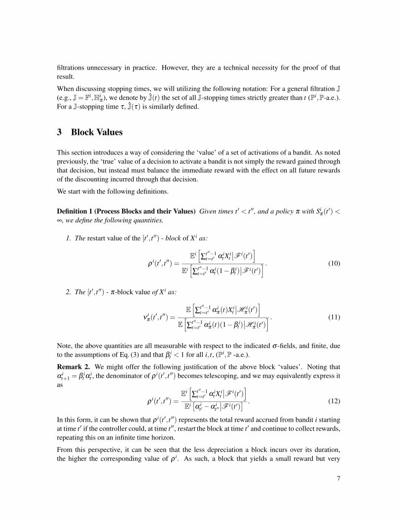
This section introduces a way of considering the ‘value’ of a set of activations of a bandit. As notedpreviously, the ‘true’ value of a decision to activate a bandit is not simply the reward gained throughthat decision, but instead must balance the immediate reward with the effect on all future rewardsof the discounting incurred through that decision.

We start with the following definitions.

Definition 1 (Process Blocks and their Values) Given times t ′ < t ′′, and a policy π with Siπ(t′) <

∞, we define the following quantities.

1. The restart value of the [t ′, t ′′) - block of X i as:

ρi(t ′, t ′′) =

Ei[∑

t ′′−1t=t ′ α i

t Xit

∣∣F i(t ′)]

Ei[∑

t ′′−1t=t ′ α i

t (1−β it )∣∣F i(t ′)

] . (10)

2. The [t ′, t ′′) - π-block value of X i as:

νiπ(t′, t ′′) =

E[∑

t ′′−1t=t ′ α i

π(t)Xit

∣∣H iπ (t′)]

E[∑

t ′′−1t=t ′ α i

π(t)(1−β it )∣∣H i

π (t ′)] . (11)

Note, the above quantities are all measurable with respect to the indicated σ -fields, and finite, dueto the assumptions of Eq. (3) and that β i

t < 1 for all i, t, (Pi,P -a.e.).

Remark 2. We might offer the following justification of the above block ‘values’. Noting thatα i

t+1 = β it α i

t , the denominator of ρ i(t ′, t ′′) becomes telescoping, and we may equivalently express itas

ρi(t ′, t ′′) =

Ei[∑

t ′′−1t=t ′ α i

t Xit

∣∣F i(t ′)]

Ei[α i

t ′−α it ′′∣∣F i(t ′)

] . (12)

In this form, it can be shown that ρ i(t ′, t ′′) represents the total reward accrued from bandit i startingat time t ′ if the controller could, at time t ′′, restart the block at time t ′ and continue to collect rewards,repeating this on an infinite time horizon.

From this perspective, it can be seen that the less depreciation a block incurs over its duration,the higher the corresponding value of ρ i. As such, a block that yields a small reward but very

7

little depreciation might in fact have a higher value than a block yielding high reward but incurringserious depreciation. This seems to capture the balance the controller must strike, between rewardand depreciation - and indeed does so, as the optimal policy will demonstrate.

Note, ν iπ as in Eq. (11) is the obvious policy-dependent generalization of ρ i in Eq. (10), rather than

ρ i as in Eq. (12). It has no immediate ‘restart’-type interpretation in this form. Taking view that theπ-block value ν i

π is the value of a block of X i when activated under a specific policy π , ρ i shouldbe viewed as the value of a block with respect to consecutive activation.

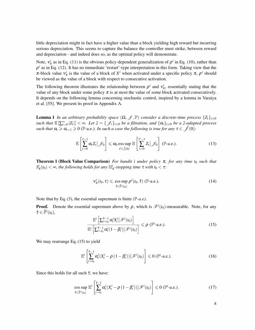
The following theorem illustrates the relationship between ρ i and ν iπ , essentially stating that the

value of any block under some policy π is at most the value of some block activated consecutively.It depends on the following lemma concerning stochastic control, inspired by a lemma in Varaiyaet al. [55]. We present its proof in Appendix A.

Lemma 1 In an arbitrary probability space (Ω,J ,P) consider a discrete-time process Ztt>0such that E [∑∞

t=0 |Zt |] < ∞. Let J = Jtt>0 be a filtration, and αtt>0 be a J-adapted processsuch that αt > αt+1 > 0 (P-a.e.). In such a case the following is true for any τ ∈ J (0):

E

[τ−1

∑t=0

αtZt∣∣J0

]6 α0 ess sup

τ ′∈J(0)E

[τ ′−1

∑t=0

Zt∣∣J0

](P-a.e.). (13)

Theorem 1 (Block Value Comparison) For bandit i under policy π , for any time t0 such thatSi

π(t0)< ∞, the following holds for any Hiπ -stopping time τ with t0 < τ:

νiπ(t0,τ)6 ess sup

τ∈Fi(t0)ρ

i(t0, τ) (P-a.e.). (14)

Note that by Eq. (3), the essential supremum is finite (P-a.e).

Proof. Denote the essential supremum above by ρ , which is F i(t0)-measurable. Note, for anyτ ∈ Fi(t0),

Ei[∑

τ−1t=t0 α i

t Xit

∣∣F i(t0)]

Ei[∑

τ−1t=t0 α i

t (1−β it )∣∣F i(t0)

] 6 ρ (Pi-a.e.). (15)

We may rearrange Eq. (15) to yield

Ei

[τ−1

∑t=t0

αit (X

it −ρ (1−β

it ))∣∣F i(t0)

]6 0 (Pi-a.e.). (16)

Since this holds for all such τ , we have:

ess supτ∈Fi(t0)

Ei

[τ−1

∑t=t0

αit (X

it −ρ (1−β

it ))∣∣F i(t0)

]6 0 (Pi-a.e.). (17)

8

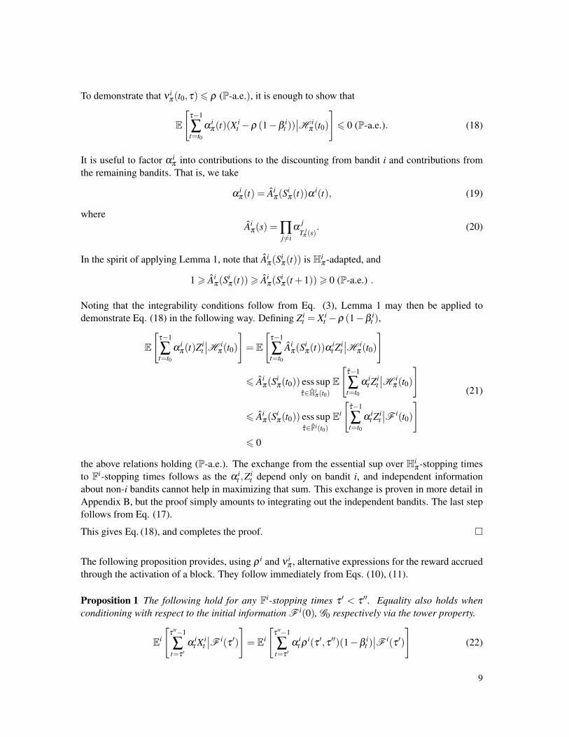
To demonstrate that ν iπ(t0,τ)6 ρ (P-a.e.), it is enough to show that

E

[τ−1

∑t=t0

αiπ(t)(X

it −ρ (1−β

it ))∣∣H i

π (t0)

]6 0 (P-a.e.). (18)

It is useful to factor α iπ into contributions to the discounting from bandit i and contributions from

the remaining bandits. That is, we take

αiπ(t) = Ai

π(Siπ(t))α

i(t), (19)

whereAi

π(s) = ∏j 6=i

αj

T jπ (s)

. (20)

In the spirit of applying Lemma 1, note that Aiπ(S

iπ(t)) is Hi

π -adapted, and

1> Aiπ(S

iπ(t))> Ai

π(Siπ(t +1))> 0 (P-a.e.) .

Noting that the integrability conditions follow from Eq. (3), Lemma 1 may then be applied todemonstrate Eq. (18) in the following way. Defining Zi

t = X it −ρ (1−β i

t ),

E

[τ−1

∑t=t0

αiπ(t)Z

it

∣∣H iπ (t0)

]= E

[τ−1

∑t=t0

Aiπ(S

iπ(t))α

it Z

it

∣∣H iπ (t0)

]

6 Aiπ(S

iπ(t0)) ess sup

τ∈Hiπ (t0)

E

[τ−1

∑t=t0

αit Z

it

∣∣H iπ (t0)

]

6 Aiπ(S

iπ(t0)) ess sup

τ∈Fi(t0)Ei

[τ−1

∑t=t0

αit Z

it

∣∣F i(t0)

]6 0

(21)

the above relations holding (P-a.e.). The exchange from the essential sup over Hiπ -stopping times

to Fi-stopping times follows as the α it ,Z

it depend only on bandit i, and independent information

about non-i bandits cannot help in maximizing that sum. This exchange is proven in more detail inAppendix B, but the proof simply amounts to integrating out the independent bandits. The last stepfollows from Eq. (17).

This gives Eq. (18), and completes the proof.

The following proposition provides, using ρ i and ν iπ , alternative expressions for the reward accrued

through the activation of a block. They follow immediately from Eqs. (10), (11).

Proposition 1 The following hold for any Fi-stopping times τ ′ < τ ′′. Equality also holds whenconditioning with respect to the initial information F i(0), G0 respectively via the tower property.

Ei

[τ ′′−1

∑t=τ ′

αit X

it

∣∣F i(τ ′)

]= Ei

[τ ′′−1

∑t=τ ′

αit ρ

i(τ ′,τ ′′)(1−βit )∣∣F i(τ ′)

](22)

9

E

[τ ′′−1

∑t=τ ′

αit X

it

∣∣H iπ (τ′)

]= E

[τ ′′−1

∑t=τ ′

αit ρ

i(τ ′,τ ′′)(1−βit )∣∣H i

π (τ′)

](23)

E

[τ ′′−1

∑t=τ ′

αiπ(t)X

it

∣∣H iπ (τ′)

]= E

[τ ′′−1

∑t=τ ′

αiπ(t)ν

iπ(τ′,τ ′′)(1−β

it )∣∣H i

π (τ′)

](24)

Remark 3. Note the relationship the above suggests between X it and ρ i(τ ′,τ ′′)(1−β i

t ), and betweenX i

t and ν iπ(τ′,τ ′′)(1−β i

t ) under π , for τ ′ 6 t < τ ′′. This will prove to be central to the final proof.

4 The Restart - in - State Index: Definition and Properties

Theorem 1 indicates the significance of the following quantity.

Definition 2 (The Restart-in-State Index) For any t < ∞, the Restart-in-State Index at t is definedto be

ρi(t) = ess sup

τ∈Fi(t)ρ

i(t,τ). (25)

This form of the index, based on the quotient in Eq. (10), was anticipated by Sonin [49], who definedit on Markov chain reward processes as a generalization of the classical Gittins dynamic allocationindex, and as an extension of the restart-in-state index of Katehakis and Veinott [37]. Note that if allthe discount factors are equal across bandits, i.e., β i

t = β for some β , for all i, and t, then this indexdiffers from the classical Gittins index by merely a factor of 1/(1−β ), and index policies based oneither index will be equivalent. However, taking β i

t in its full generality, no such relationship existsbetween the indices and therefore between policies.

The necessity of the restart-in-state index, within the discrete time model framework, is establishedby example in Section 4.1.

Noting that ρ i(t,τ) is the value of the [t,τ) - block, we may interpret ρ i(t) as the maximal blockvalue achievable from bandit i from time t. The use of the terms maximal and achievable is justifiedhere as ρ i(t) is realized (Pi-a.e.) as the value of some block starting at t. To show this requiresthe following technical lemma, which follows as a special case of classic results of Snell [47] andothers, cf. the Optional Stopping Lemma of Derman and Sacks [16] and its discussion in Katehakiset al. [35].

Lemma 2 In an arbitrary probability space, consider a discrete-time process Ztt>0 such thatE [∑∞

t=0 |Zt |]< ∞. Let J= Jtt>0 be a filtration such that the Zt are J-adapted. Then, there existsa (potentially infinite) stopping time τ∗ ∈ J(0) such that

E

[τ∗−1

∑t=0

Zt

∣∣∣J0

]= ess sup

τ∈J(0)E

[τ−1

∑t=0

Zt

∣∣∣J0

](P-a.e.). (26)

In particular, we may take

τ∗ = infn > 0 : ess sup

τ∈J(n)E

[τ−1

∑t=n

Zt∣∣Jn

]< 0. (27)

10

Note, we allow infinite stopping times, as the sum in Eq. (27) is well defined by assumption.

Utilizing this lemma, we have the following result.

Proposition 2 For any time t0 < ∞, there exists a τ ∈ Fi(t0) such that ρ i(t0) = ρ i(t0,τ) (Pi-a.e.).

Proof. We have that for all τ ∈ Fi(t0), ρ i(t0, τ)6 ρ i(t0) (Pi-a.e.), or in parallel with Eq. (16),

Ei

[τ−1

∑t=t0

αit(X i

t −ρi(t0)(1−β

it ))∣∣F i(t0)

]6 0 (Pi-a.e.). (28)

Defining

ε =− ess supτ∈Fi(t0)

Ei

[τ−1

∑t=t0

αit(X i

t −ρi(t0)(1−β

it ))∣∣F i(t0)

], (29)

we have that ε > 0 (Pi-a.e.). We may use −ε as an improved upper bound in Eq. (28). This may berearranged to yield

ρi(t0, τ)6 ρ

i(t0)−ε

Ei[∑

τ−1t=t0 α i

t (1−β it )∣∣F i(t0)

]= ρ

i(t0)−ε

Ei[α i

t0−α iτ

∣∣F i(t0)]

6 ρi(t0)− ε (Pi-a.e.).

(30)

Since the above property holds for all such τ , it extends to the essential supremum, yielding

ρi(t0)6 ρ

i(t0)− ε (Pi-a.e.), (31)

or equivalently that ε 6 0 (Pi-a.e.). In conjunction with the first observation, that ε > 0 (Pi-a.e.), wehave ε = 0 (Pi-a.e.), i.e.,

ess supτ∈Fi(t0)

Ei

[τ−1

∑t=t0

αit(X i

t −ρi(t0)(1−β

it ))∣∣F i(t0)

]= 0 (Pi-a.e.). (32)

To satisfy the hypotheses of Lemma 2, note that the integrability stems by the assumption of (3).We may apply Lemma 2 in this instance to yield a stopping time τ∗ ∈ Fi(t0) such that

Ei

[τ∗−1

∑t=t0

αit(X i

t −ρi(t0)(1−β

it ))∣∣F i(t0)

]= 0 (Pi-a.e.), (33)

or

ρi(t0) =

Ei[∑

τ∗−1t=t0 α i

t Xit

∣∣F i(t0)]

Ei[∑

τ∗−1t=t0 α i

t (1−β it )∣∣F i(t0)

] = ρi(t0,τ∗) (Pi-a.e.). (34)

11

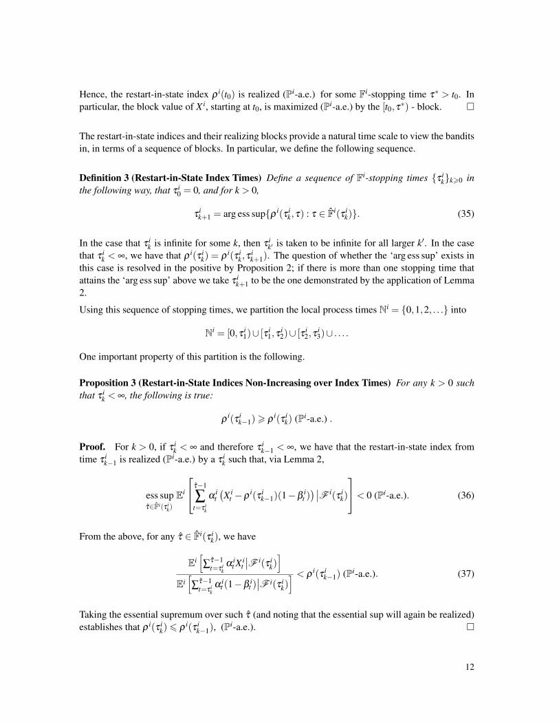
Hence, the restart-in-state index ρ i(t0) is realized (Pi-a.e.) for some Fi-stopping time τ∗ > t0. Inparticular, the block value of X i, starting at t0, is maximized (Pi-a.e.) by the [t0,τ∗) - block.

The restart-in-state indices and their realizing blocks provide a natural time scale to view the banditsin, in terms of a sequence of blocks. In particular, we define the following sequence.

Definition 3 (Restart-in-State Index Times) Define a sequence of Fi-stopping times τ ikk>0 in

the following way, that τ i0 = 0, and for k > 0,

τik+1 = arg ess supρ i(τ i

k,τ) : τ ∈ Fi(τ ik). (35)

In the case that τ ik is infinite for some k, then τ i

k′ is taken to be infinite for all larger k′. In the casethat τ i

k < ∞, we have that ρ i(τ ik) = ρ i(τ i

k,τik+1). The question of whether the ‘arg ess sup’ exists in

this case is resolved in the positive by Proposition 2; if there is more than one stopping time thatattains the ‘arg ess sup’ above we take τ i

k+1 to be the one demonstrated by the application of Lemma2.

Using this sequence of stopping times, we partition the local process times Ni = 0,1,2, . . . into

Ni = [0,τ i1)∪ [τ i

1,τi2)∪ [τ i

2,τi3)∪ . . . .

One important property of this partition is the following.

Proposition 3 (Restart-in-State Indices Non-Increasing over Index Times) For any k > 0 suchthat τ i

k < ∞, the following is true:

ρi(τ i

k−1)> ρi(τ i

k) (Pi-a.e.) .

Proof. For k > 0, if τ ik < ∞ and therefore τ i

k−1 < ∞, we have that the restart-in-state index fromtime τ i

k−1 is realized (Pi-a.e.) by a τ ik such that, via Lemma 2,

ess supτ∈Fi(τ i

k)

Ei

τ−1

∑t=τ i

k

αit(X i

t −ρi(τ i

k−1)(1−βit ))∣∣F i(τ i

k)

< 0 (Pi-a.e.). (36)

From the above, for any τ ∈ Fi(τ ik), we have

Ei[∑

τ−1t=τ i

kα i

t Xit

∣∣F i(τ ik)]

Ei[∑

τ−1t=τ i

kα i

t (1−β it )∣∣F i(τ i

k)] < ρ

i(τ ik−1) (Pi-a.e.). (37)

Taking the essential supremum over such τ (and noting that the essential sup will again be realized)establishes that ρ i(τ i

k)6 ρ i(τ ik−1), (Pi-a.e.).

12

4.1 Necessity of the restart in state indices

We construct the following toy example to demonstrates the inapplicability of the classical form ofthe dynamic allocation (Gittins) indices, within the discrete time model framework. Suppose thecontroller is given two deterministic, finite processes, X1 = 1,2 and X2 = 100; they can alsobe thought of as infinite processes with infinite trailing 0’s. Further, each activation of X1 incurs adiscount factor of a (i.e., β 1

0 = β 11 = a) and each activation of X2 incurs a discount factor of b (i.e.,

β 20 = b) with a, b ∈ (0,1).

The classic Gittins(1979) DAI dynamic allocation indices of X1 and X2 at s = 0 are: γX1 = (1+2a)/(1+a) = max1/1 ,(1+2a)/(1+a) and γX2 = 100. From this, it is clear that for any valueof a ∈ (0,1), γX1 < γX2 . Hence, the DAI based dynamic allocation policy specifies to activate X2

first, then X1 twice. This gives a value of VDAI = 100+1b+2ab. However, consider the alternativestrategy of activating X1 twice first, then activating X2. This gives a value of V ′ = 1+2a+100a2.Comparing the two, we have

V ′−VDAI

(1−b)(1−a2)=

1+2a1−a2 −

1001−b

.

It is clear from the above that for a especially large and b small, the difference in values is positive,and the policy determined by the restart dynamic allocation indices is in fact superior in value tothe policy determined by the DAI indices, i.e., the traditional DAI policy may specify a non-optimalpolicy. On the other hand, it is easy to see that the policy based on the restart in state indices ofX1 and X2 which at s = 0 are: ρX1 = (1 + 2a)/(1− a2) = max1/(1− a),(1 + 2a)/(1− a2),ρX2 = 100/(1−b) is always optimal.

5 Bandit and Policy Equivalent Reward Processes

For each bandit, we have developed a partition of local time for into blocks of activations, via therestart-in-state index stopping times. We extend on the remarks at the end of Section 3, by definingthe following alternative reward processes.

Definition 4 Given the collection of reward processes X = (X1,X2, . . . ,XN), discount factor se-quences B= (β 1,β 2, . . . ,β N), and τ i

kk>0 as by Definition 3, we define:

1. The reward-equivalent collection YX = (Y 1, ...,Y N) by

Y i(t) = ρi(τ i

k)(1−βit ), if τ

ik 6 t < τ

ik+1. (38)

2. For π ∈P , the π-equivalent collection YXπ = (Y 1

π , ...,YNπ ), by

Y iπ(t) = ν

iπ(τ

ik,τ

ik+1)(1−β

it ), if τ

ik 6 t < τ

ik+1. (39)

Like X i, the process Y i is defined on (Ωi,F i,Pi,Fi) and is Fi-adapted, as ρ i(τ ik) is defined by the

information available locally at time τ ik. However, as the ν i

π(τik,τ

ik+1) depend on the specifics of a

13

policy π , so do the Y iπ processes; the Y i

π processes are Hiπ -adapted, but not Fi-adapted. Note that,

should bandit i be activated only finitely many times under π , Y iπ will only really be defined up to

some τ ik+1 such that Si

π(τik+1) = ∞. For such undefined Y i

π(t), we take 0∗Y iπ(t) = 0.

The following are simple, but important, properties of the Y i,Y iπ processes.

Proposition 4 For each bandit i, the following hold any k > 0:

Ei

τ ik+1−1

∑t=τ i

k

αit X

it

∣∣F i(τ ik)

= Ei

τ ik+1−1

∑t=τ i

k

αitY

i(t)∣∣F i(τ i

k)

, (40)

E

τ ik+1−1

∑t=τ i

k

αit X

it

∣∣H iπ (τ

ik)

= E

τ ik+1−1

∑t=τ i

k

αitY

i(t)∣∣H i

π (τik)

, (41)

E

τ ik+1−1

∑t=τ i

k

αiπ(t)X

it

∣∣H iπ (τ

ik)

= E

τ ik+1−1

∑t=τ i

k

αiπ(t)Y

iπ(t)

∣∣H iπ (τ

ik)

. (42)

As with Proposition 1, equality also holds when conditioning with respect to F i(0),G0.

Proof. This follows as an application of Proposition 1 and the definitions of Y i, Y iπ .

The following proposition serves as a justification of the term ‘equivalent’ to describe Y i,Y iπ .

Proposition 5 For each bandit i,

Ei

[∞

∑t=0

αit X

it

∣∣F i(0)

]= Ei

[∞

∑t=0

αitY

i(t)∣∣F i(0)

], (43)

E

[∞

∑t=0

αiπ(t)X

it

∣∣G0

]= E

[∞

∑t=0

αiπ(t)Y

iπ(t)

∣∣G0

]. (44)

Proof. Each follows from the corresponding equation in Prop. 4, summing over k and takingexpectations from the initial time, via the tower property.

Theorem 2 (Comparison of the Equivalent Processes) For each i and all time t, we have:

αiπ(t)Y

iπ(t)6 α

iπ(t)Y

i(t) (P-a.e.). (45)

Proof. If the controller does not activate bandit i at least t times under π , ever (i.e., Siπ(t) = ∞),

then some bandit j 6= i must be activated infinitely many times under π . As such, α iπ(t) 6 α j

∞ = 0,by Eq. (2). Hence, α i

π(t) = 0, and the inequality holds.

14

If the controller does activate bandit i at least t times under π , then α iπ(t) is non-zero and can be

ignored on both sides of the inequality. In that case, we have for some k that τ ik 6 t < τ i

k+1, and asan application of Theorem 1,

Y iπ(t) = ν

iπ(τ

ik,τ

ik+1)(1−β

it )6 ρ

i(τ ik)(1−β

it ) = Y i(t) (P-a.e.). (46)

6 A Greedy Result and the Optimal Control Policy

The importance of the YX collection is that the optimal policy for these reward processes may bederived with relative ease. In fact, for these processes, not only may the total reward be maximizedin expectation, but a policy exists which maximizes the reward almost surely. That is, we have thefollowing theorem.

Theorem 3 (Pointwise Optimization on YX Processes) Given a reward - discount pair (X,B), letYX be the collection of reward-equivalent processes. There exists a policy π∗ ∈P such that forany other policy π ∈P , π∗ yields a greater total reward, almost surely. That is, defining Y X

π (s) =Y π(s)(Tπ(s)),

∞

∑s=0

Aπ(s)Y Xπ (s)6

∞

∑s=0

Aπ∗(s)Y Xπ∗(s) (P-a.e.). (47)

In particular, such a π∗ is given by the following rule: Activate bandit i corresponding to the largestcurrent value of ρ i(τ i

k), for a duration corresponding to the realizing [τ ik,τ

ik+1)-block, repeating this

ad infinitum.

Proof. Without loss of generality, let ρ1(0)> ρ i(0) for all i. Since the ρ i(τ ik) are decreasing with

k, we have for all i,k thatρ

1(0)> ρi(τ i

k) (P-a.e.). (48)

Let π be an arbitrary policy in P , and define S = S1π(0), the first time bandit 1 is activated under π .

Note, if bandit 1 is never activated, we take S to be infinite.

We may express the total reward under π sample path wise as

Rπ =∞

∑s=0

Aπ(s)Y Xπ (s)

=S−1

∑s=0

Aπ(s)Y Xπ (s)+Aπ(S)Y 1(0)+

∞

∑s=S+1

Aπ(s)Y Xπ (s)

(49)

From π , we construct a policy π ′ ∈P in the following way: π ′ is identical to π in that it activatesbandits in the same order, but it advances the first activation of bandit i from round s = S to round

15

s = 0. That is,

π′(s) =

1 for s = 0,π(s−1) for s = 1,2, . . .S,π(s) for s> S+1.

(50)

It is important to observe that π ′ is in P , as at every round s, the information available under π ′ isgreater than or equal to the information available under π .

Using this relation, we may express the sample path wise reward under policy π ′, relative to π , as

Rπ ′ =∞

∑s=0

Aπ ′(s)Y Xπ ′ (s)

= Y 1(0)+S

∑s=1

Aπ ′(s)Y Xπ ′ (s)+

∞

∑s=S+1

Aπ ′(s)Y Xπ ′ (s)

= Y 1(0)+S

∑s=1

β10 Aπ(s−1)Y X

π (s−1)+∞

∑s=S+1

Aπ(s)Y Xπ (s)

= Y 1(0)+β10

S−1

∑s=0

Aπ(s)Y Xπ (s)+

∞

∑s=S+1

Aπ(s)Y Xπ (s).

(51)

Comparing the two, we have

Rπ ′−Rπ =

(Y 1(0)+β

10

S−1

∑s=0

Aπ(s)Y Xπ (s)

)−

(S−1

∑s=0

Aπ(s)Y Xπ (s)+Aπ(S)Y 1(0)

)

= Y 1(0)(1−Aπ(S))− (1−β10 )

S−1

∑s=0

Aπ(s)Y Xπ (s)

= Y 1(0)(1−Aπ(S))−S−1

∑s=0

Aπ(s)(1−β10 )Y

Xπ (s).

(52)

Defining βπ(s) = βπ(s)Tπ (s)

, we have by Eq. (48) that (1−β 10 )Y

Xπ (s)6 (1−βπ(s))Y 1(0). Hence,

Rπ ′−Rπ > Y 1(0)(1−Aπ(S))−S−1

∑s=0

Aπ(s)(1−βπ(s))Y 1(0)

= Y 1(0)(1−Aπ(S))−Y 1(0)S−1

∑s=0

(Aπ(s)−Aπ(s)βπ(s))

= Y 1(0)(1−Aπ(S))−Y 1(0)S−1

∑s=0

(Aπ(s)−Aπ(s+1))

= Y 1(0)(1−Aπ(S))−Y 1(0)(1−Aπ(S))

= 0 (P-a.e.).

(53)

Immediately, for any policy π , advancing the first activation of the bandit with the largest currentρ i value almost surely increases, or does not change, the value of the policy. This argument can be

16

extended, via a forward induction type argument, to show that any finite number of these ρ-greedyadvancements almost surely improves or does not change the value of the policy. Collisions, whentwo bandits have the same current ρ-value, are left to the discretion of the controller, but may beresolved with a simple rule such as always picking the lowest numbered bandit.

It remains to compare these improved strategies to the completely ρ-greedy strategy as in the theo-rem. Let π∗ ∈P be the completely ρ-greedy strategy, described in the theorem. For a given π ∈P ,let πN ∈P be the policy that results from π after N-many ρ-greedy advancements. Notice, π∗ andπN agree for the first N rounds. Let τ i

N = T iπ∗(N). Recalling the definition of Ai

π(s), cf. Eq. (20), asthe discounting due to non-i bandits at round s, we have the following bound:

|Rπ∗−RπN |6N

∑i=1

∞

∑t=τ i

N

|α iπ∗(t)−α

iπN(t)||Y i(t)|

6N

∑i=1

∞

∑t=τ i

N

αit A

iπ∗(S

iπ∗(τ

iN))|Y i(t)|

6N

∑i=1

Aiπ∗(S

iπ∗(τ

iN))

∞

∑t=τ i

N

αit |Y i(t)|

.

(54)

Note that it follows from the definition of Y i and Eq. (3) that ∑∞t=0 α i

t |Y i(t)|< ∞ (Pi-a.e.).

For a given bandit i under π∗, two things may happen: either i is activated infinitely many times, ori is activated finitely many times.

If i is activated infinitely many times under π∗, then τ iN increases without bound with N. As such,

∑∞

t=τ iN

α it |Y i(t)| converges to 0 (P-a.e.) . As the depreciation due to the non-i bandits is at most 1,

the contribution of bandit i in the above sum converges to 0 with N.

If i is activated finitely many times under π∗, then some bandit j 6= i is activated infinitely manytimes under π∗. Thus, for some finite N, Si

π∗(τiN) = ∞, and for the infinitely activated bandit j 6= i

we have Aiπ∗(S

iπ∗(τ

iN)) 6 α j

∞ = 0 (P-a.e.), by Eqs. (2) and (20). In other words, the depreciationincurred at infinity is at most the depreciation incurred from j at infinity, which is 0. Since the totalremaining reward from bandit i is finite almost surely, the contribution of bandit i to the above sumconverges to 0 with N (P-a.e.).

The above imply the following,

limN→∞|Rπ∗−RπN |= 0 (P-a.e.). (55)

Since the value of any policy may be improved by a finite number of ρ-greedy advancements, andthe value of a policy under N ρ-greedy advancements converges to the value of the total ρ-greedypolicy π∗, it follows that for any policy π ∈P we have (P-a.e.) that Rπ 6 Rπ∗ , verifying the theo-rem.

Remark 4. An important feature of the optimal policy π∗ for the YX processes is that it preservesrestart in state index blocks. Because it is ρ-greedy, we have explicitly, for τ i

k 6 τ ik + t < τ i

k+1, that

17

π∗(Siπ∗(τ

ik)+ t) = i, (P-a.e.).

We then have the following result.

Theorem 4 (The Optimal Control Policy for Generalized Deprecation) For a collection of re-ward processes X = (X1,X2, . . . ,XN), and discount factor sequences B = (β 1,β 2, . . . ,β N), thereexists a strategy π∗ ∈P such that for all π ∈P ,

Vπ(X,B)6Vπ∗(X,B) (P-a.e.). (56)

In particular, such an optimal π∗ can be described in the following way: Successively, activate thebandit with the largest restart in state index ρ i, for the duration of the corresponding index block.

Proof. For an arbitrary policy π , and π∗ as indicated above, we establish the following relations:

Vπ(X,B) =Vπ(YXπ ,B)6Vπ(YX ,B)6Vπ∗(YX ,B) =Vπ∗(X,B) (P-a.e.), (57)

i.e., for any policy π , we have that Vπ(X,B) 6 Vπ∗(X,B) (P-a.e.) and therefore π∗ is an optimalpolicy. In the following steps we prove relations (57).

Step 1: Vπ(X,B) =Vπ(YXπ ,B), (P-a.e.).

We have, by Proposition 5,

Vπ(X,B) =N

∑i=1

E

[∞

∑t=0

αiπ(t)X

it

∣∣G0

]=

N

∑i=1

E

[∞

∑t=0

αiπ(t)Y

iπ(t)

∣∣G0

]=Vπ(YX

π ,B).

Note, because the Y iπ processes are defined in terms of π , they are not Fi-adapted, and cannot be

utilized under any other policy. However, the value Vπ(YXπ ) is well defined via the above equation.

Step 2: Vπ(YXπ ,B)6Vπ(YX ,B) (P-a.e.).

This follows simply from the almost sure comparison of Theorem 2, giving

Vπ(YXπ ,B) =

N

∑i=1

E

[∞

∑t=0

αiπ(t)Y

iπ(t)

∣∣G0

]6

N

∑i=1

E

[∞

∑t=0

αiπ(t)Y

i(t)∣∣G0

]=Vπ(YX ,B). (58)

Step 3: Vπ(YX ,B)6Vπ∗(YX ,B) (P-a.e.).

This is simply an application of Theorem 3, as Vπ(YX ,B) = E [Rπ |G0], with Rπ as in the theorem.

Step 4: Vπ∗(YX ,B) =Vπ∗(X,B) (P-a.e.).

By the factorization of α iπ(t) as in Eq. (19), and Remark 4, we may express the total reward under

π∗ relative to the [τ ik,τ

ik+1)-blocks. In this way, we may apply Proposition 4 to yield the following

equivalence,

Vπ∗(YX ,B) =N

∑i=1

∞

∑k=0

E

Aiπ(S

iπ(τ

ik))E

τ ik+1−1

∑t=τ i

k

αitY

i(t)∣∣H i

π (τik)

∣∣G0

=

N

∑i=1

∞

∑k=0

E

Aiπ(S

iπ(τ

ik))E

τ ik+1−1

∑t=τ i

k

αit X

it

∣∣H iπ (τ

ik)

∣∣G0

=Vπ∗(X,B) (P-a.e.).

18

This completes the proof.

Remark 5. The above theorem demonstrates a policy π∗ ∈P that is P-a.e. superior (or equivalent)to every other policy π ∈P . However, the set of non-anticipatory policies P was defined in a fairlyrestrictive sense in Sec. 2.1, so that the decision in any round was completely determined by theresults of the past. This might be weakened to allow for randomized policies, so that the decisionin a given round might depend on the results of independent events, e.g., coin flips. However, sucha construction simply amounts to placing a distribution on P . Since π∗ is P-a.e. superior to anyπ ∈P , π∗ would be similarly superior to any policy sampled randomly from P .

7 A Model of Commitments

One way of interpreting the discount factor β it in the previous model is as related to the duration

of the tth activation of bandit i - durations that may be non-uniform across bandits, and acrosstime. This section lays out this relationship in detail: We define a continuous time model, in whichrewards are discounted continuously at a fixed rate, and in which activation of a bandit is subject toa (potentially stochastic) period of commitment that must pass before the controller is again free toselect a bandit to activate. Such commitments might arise as the product of contractual obligations,or properties of the bandits such as operational speeds, or the controller may simply require a certaincondition be met before switching.

The key assumptions are again that the bandits are independent, and unactivated bandits remainfrozen. The controller’s goal remains the maximization her expected total reward. As such, eachdecision of which bandit to activate must balance not only the immediate reward collected, butpotential delay in collection and additional discounting of all future rewards, due to commitment.

A controller is presented with a collection of filtered probability spaces, (Ωi,F i,Pi,Fi), for 1 6i 6 N < ∞, each indexed in continuous time, and satisfying the usual conditions. To each space,we associate a continuous time reward rate process X i = X i

t t>0. For t ∈ [0,∞), we take X it (=

X it (ω

i)) ∈ R to represent the reward rate received from bandit i at time t during its activation.Rewards are discounted at a fixed rate r > 0, compounded continuously. We take X i to be Fi-adapted, and denote the collection of reward processes as X.

Additionally, to each bandit we associate a commitment process ci = cikk>0. Commitment pro-

cesses function in the following way: When bandit i is activated for the kth time, it must be continu-ously activated for a duration of ci

k(ωi) ∈ R+ before the controller is again free to activate from the

N bandits as she chooses. We will refer to cik as the duration of the kth commitment epoch of bandit

i. We denote the collection of commitment processes as C.

For each bandit, it is convenient to define a sequence Cikk>0 of process epoch times by Ci

0 = 0,and Ci

k = ∑k−1k′=0 ci

k′ . Note that Cik gives the ‘local’ time at which the kth activation epoch of bandit i

begins. In addition to the assumption that X i is Fi-adapted, we take each cik as F i(Ci

k)-measurable,i.e., the duration of a given epoch is determined by all the results prior to the start of that epoch.Note then that the Ci

k represent Fi-stopping times.

In addition to Assumptions A and B, we take the following additional restrictions on each bandit i.

19

Assumption C′.

limk→∞

Cik =

∞

∑k=0

cik = ∞ (Pi-a.e.), (59)

and

Ei[∫

∞

0e−rt |X i

t |dt]< ∞. (60)

The former restriction implies the total time of each bandit is infinite, and the latter again impliesthat the expected total reward from any one bandit is finite.

A control policy π now becomes a right-continuous stochastic process on the global space, suchthat π(s) = i means the controller is activating bandit i at global time s. Note, in continuous time,the use of ‘round’ to describe a unit of global time is no longer sensible.

Given a policy π , we may define continuous time versions of T iπ(s) and Si

π(t) as

T iπ(s) =

∫ s

01π(s′)=ids′, (61)

and, utilizing the above,Si

π(t) = infs> 0 : T iπ(s)> t. (62)

Extending the ideas of Section 2.1, we define a policy π to be non-anticipatory if for s > 0, π(s)is measurable with respect to

⊗Ni=1 F i(T i

π(s)). However, we are only interested in the set PC ofnon-anticipatory policies π that satisfy the commitment constraints, i.e., for each bandit i, for eachk > 0,

Siπ(C

ik + t) = Si

π(Cik)+ t, for 06 t < ci

k,

π(Siπ(C

ik + t)) = i, for all 06 t < ci

k.(63)

In parallel with the previous sections, we let VCπ (X,C) denote the value of a policy, the expected

total reward given the reward-commitment pair (X,C) under policy π ∈PC. We may thereforeexpress the value of a policy as

VCπ (X,C) = E

[∫∞

0e−rsXπ(s)ds

∣∣G0

], (64)

relative to global time, or relative to local time as

VCπ (X,C) =

N

∑i=1

E[∫

∞

0e−rSi

π (t)X it dt∣∣G0

]. (65)

The problem the controller faces is to determine a policy π∗ ∈PC that is optimal in the sense that,for any other π ∈PC,

VCπ (X,C)6VC

π∗(X,C) (P-a.e.). (66)

We resolve this be reducing this commitment model to the previous depreciation model. That is, wehave the following result.

20

Theorem 5 Given a collection of bandits (Ωi,F i,Pi,Fi)16i6N in continuous time, with the reward-commitment pair (X,C), there exists a collection of bandits (Ωi,F i,Pi, Fi)16i6N in discrete time,with the reward-discount pair (X, B), such that for any policy π ∈PC, there exists a policy π ∈Psuch that

VCπ (X,C) =Vπ(X, B) (P-a.e.), (67)

and vice versa, such a π ∈PC exists for any π ∈P .

Proof. The construction is fairly natural, amounting to a translation from the continuous ‘commit-ment time’ to a discrete ‘decision time’, in which one unit of time indicates a single decision by thecontroller. To the kth activation of bandit i, we associate the following quantities:

X ik := Ei

[∫ cik

0e−rtX i

Cik+tdt

∣∣F i(Cik)

],

βik := e−rci

k ,

F i(k) := F i(Cik).

(68)

These represent, respectively, the expected reward collected during the kth commitment period, thedepreciation incurred on all future rewards due to the kth commitment period, and the informationavailable about bandit i prior to the kth decision to activate it. These define, therefore, a discretetime reward process X i = X i

kk>0, a discount factor sequence β i = β ikk>0, and a discrete time

filtration Fi = F i(k)k>0 to which they are both adapted. We may then define the total depreciationsequence α i = α i

kk>0 by Eq. (1) using β i, which yields α ik = e−rCi

k . Observe then that we havethe following,

limk→∞

αik = lim

k→∞

e−rCik = 0 (Pi-a.e.), (69)

and

Ei

[∞

∑k=0

αik|X i

k|

]6 Ei

[∞

∑k=0

∫ Cik+1

Cik

e−rt |X it |dt

]

= Ei[∫

∞

0e−rt |X i

t |dt]< ∞.

(70)

This gives us an instance (X, B) of the depreciation model on the bandits (Ωi,F i,Pi, Fi)16i6N .

Taking a policy π ∈PC on (X,C), we may translate it into a discrete time policy π ∈P on (X, B)in the following way: if the hth decision made under policy π is to activate bandit i, we haveπ(h) = i. Similarly, given a π ∈P , it may be translated into a policy π ∈PC by taking π to be thecontinuous time extension of π that satisfies the commitment periods. In this way, we may go backand forth between models. Note then, we may define the a policy dependent depreciation sequenceby α i

π(k) = e−rSi

π (Cik), the total depreciation incurred on the kth commitment period by all previous

activation.

21

Hence, given π ∈PC and the corresponding π ∈P , or vice versa,

VCπ (X,C) =

N

∑i=1

E[∫

∞

0e−rSi

π (t)X it dt∣∣G0

]=

N

∑i=1

E

[∞

∑k=0

∫ Cik+1

Cik

e−rSiπ (t)X i

t dt∣∣G0

]

=N

∑i=1

E

[∞

∑k=0

∫ cik

0e−rSi

π (Cik+t)X i

Cik+tdt

∣∣G0

]

=N

∑i=1

E

[∞

∑k=0

∫ cik

0e−r(Si

π (Cik)+t)X i

Cik+tdt

∣∣G0

]

=N

∑i=1

E

[∞

∑k=0

e−rSiπ (C

ik)∫ ci

k

0e−rtX i

Cik+tdt

∣∣G0

]

=N

∑i=1

E

[∞

∑k=0

αiπ(k)X i

k

∣∣G0

]=Vπ(X, B) (P-a.e.).

(71)

This connection between the commitment model and the depreciation model can also be used toconstruct a continuous time commitment model that is equivalent of a given depreciation model,essentially by inverting the relationships in Eq. (68), for example, taking commitment durations asci

k = − ln(β ik)/r (for a context specific choice of r > 0). In this way, it can be shown that the two

models are equivalent. This construction will not be explored further here.

Theorem 5 implies that any instance of the commitment model may be solved by translating it intothe corresponding depreciation model and solving it there, via the restart-in-state index.

The model presented above was taken to be in continuous time. A discrete time model is alsopossible, in which case future rewards are discounted by some fixed factor β ∈ (0,1) per round,and each commitment duration refers to a fixed number of activations, ci

k ∈ N. Everything done inthe continuous case goes through for the discrete with X i(k) and β i

k defined by the following as anextension of Eq. (68):

X i(k) = Ei

cik−1

∑t=0

βtX i(Ci

k + t)∣∣F i(Ci

k)

,β

ik = β

cik .

(72)

8 Assumptions C and C′, and Zeno’s Hypothesis

In both of the models presented in this paper, the individual bandits were restricted in two ways, byAssumptions C and C′. First we assumed the integrability conditions of Eqs. (3), (60), effectively

22

requiring that the total expected reward from each bandit be finite. This requirement was takensimply to ensure a degree of realism in the model.

Additionally the restrictions of Eqs. (2) and (59): ∏∞t=0 β i

t = 0, ∑∞k=0 ci

k = ∞ (Pi-a.e.) ∀i, wererespectively placed on each model as a matter of both necessity and convenience. Through the re-lationships between the models defined in Eq. (68), these assumptions were shown to be equivalentin Eq. (69).

The mathematical necessity of these assumptions arose in the proof of Theorem 3 in Eq. (54), inproving that the values of finite-step ρ-greedy policy improvements converged to the value of theinfinite ρ-greedy policy. The key point was that if a bandit were only activated finitely many timesunder a policy, the remaining rewards from that bandit were discounted to 0 by the assumption ofEq. (2).

The convenience of these assumptions can be seen most directly in the continuous time commitmentmodel. If the commitment durations of a given bandit summed to some finite value, a situation mayarise in which the controller may make infinitely many decisions in finite time. For instance takingci

k = 2−k for some i, the decisions to activate each commitment period of bandit i would only take2 units of time total. The controller would then be faced with a Zeno-type problem of making the‘next’ activation decision after an infinite sequence of activation decisions. Taking the assumptionof Eq. (59) that the total commitment time must be infinite sidesteps any potential entanglements ofthis type, guaranteeing that only finitely many decisions can be made in finite time.

From this perspective, Assumptions C and C′ can be interpreted similarly for each model: eachensures that after an infinite sequence of decisions, the value of uncollected rewards is zero - eitherthrough the infinite delay of the commitment model, or the discounting to 0 of the depreciationmodel. Hence, any decision made ‘after’ an infinite sequence of decisions contributes nothing tothe total and can be ignored.

We note that in the case of a constant discount factor for all bandits and times i.e., β it = β , and for

commitment times bounded from below i.e., cik > δ for some δ > 0, the hypotheses of Assumption

C and C′ are automatically satisfied.

Appendices

A Proof of Lemma 1

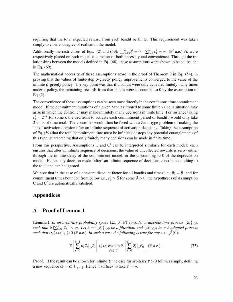
Lemma 1 In an arbitrary probability space (Ω,J ,P) consider a discrete-time process Ztt>0such that E [∑∞

t=0 |Zt |] < ∞. Let J = Jtt>0 be a filtration, and αtt>0 be a J-adapted processsuch that αt > αt+1 > 0 (P-a.e.). In such a case the following is true for any τ ∈ J (0):

E

[τ−1

∑t=0

αtZt∣∣J0

]6 α0 ess sup

τ ′∈J(0)E

[τ ′−1

∑t=0

Zt∣∣J0

](P-a.e.). (73)

Proof. If the result can be shown for infinite τ , the case for arbitrary τ > 0 follows simply, defininga new sequence αt = αt1τ>t. Hence it suffices to take τ = ∞.

23

This result follows straightforwardly in the case the Zt sequence has finitely many terms. Theresult is trivial if there is a single term. In the case of two terms,

E[α0Z0 +α1Z1

∣∣∣J0

](74)

is maximized taking α1 to be the J1-measurable random variable defined by

α1 =

α0 if E[Z1

∣∣∣J1

]> 0

0 if E[Z1

∣∣∣J1

]6 0

. (75)

In short, if the remaining contribution is positive, make α1 as large as possible (i.e., equal to α0),else make α1 as small as possible (i.e., equal to 0). Either way, this factors simply, giving in allcases,

E[α0Z0 +α1Z1

∣∣∣J0

]6 α0 ess sup

τ∈J(0),τ62E

[τ−1

∑t=0

Zt∣∣J0

](P-a.e.). (76)

We may apply this result inductively in the following way. Allowing N < ∞ terms,

E

[N−1

∑t=0

αtZt∣∣J0

]= E

[α0Z0 +E

[N−1

∑t=1

αtZt∣∣J1

]∣∣J0

]

6 E

[α0Z0 +α1 ess sup

τ∈J(1),τ6NE

[τ−1

∑t=1

Zt∣∣J1

]∣∣J0

].

(77)

Again, the optimal choice of α1 is the J1-measurable random variable given by α0 if the essentialsup is positive and 0 if it is negative. In either case, we have the following,

E

[N−1

∑t=0

αtZt∣∣J0

]6 α0 ess sup

τ∈J(0),τ6NE

[τ−1

∑t=0

Zt∣∣J0

](P-a.e.). (78)

This extends immediately to all finite, J0-measurable N. We next extend the finite result to theinfinite.

The initial assumption E [∑∞t=0 |Zt |] < ∞ implies that E [∑∞

t=0 |Zt ||J0] < ∞ (P-a.e.). Thus for anyfixed ε > 0, we may find a J0-measurable and finite N > 0 (P-a.e.) such that

E

[∞

∑t=N|Zt |∣∣J0

]6 ε (P-a.e.). (79)

24

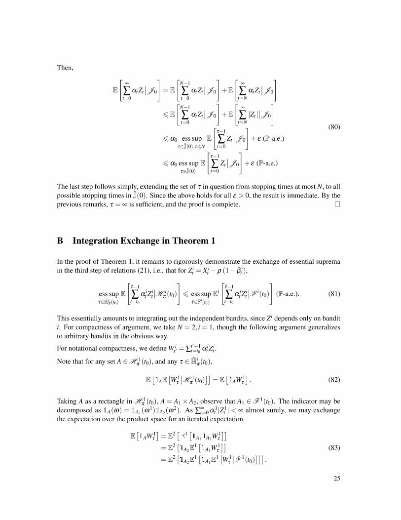
Then,

E

[∞

∑t=0

αtZt∣∣J0

]= E

[N−1

∑t=0

αtZt∣∣J0

]+E

[∞

∑t=N

αtZt∣∣J0

]

6 E

[N−1

∑t=0

αtZt∣∣J0

]+E

[∞

∑t=N|Zt |∣∣J0

]

6 α0 ess supτ∈J(0),τ6N

E

[τ−1

∑t=0

Zt∣∣J0

]+ ε (P-a.e.)

6 α0 ess supτ∈J(0)

E

[τ−1

∑t=0

Zt∣∣J0

]+ ε (P-a.e.)

(80)

The last step follows simply, extending the set of τ in question from stopping times at most N, to allpossible stopping times in J(0). Since the above holds for all ε > 0, the result is immediate. By theprevious remarks, τ = ∞ is sufficient, and the proof is complete.

B Integration Exchange in Theorem 1

In the proof of Theorem 1, it remains to rigorously demonstrate the exchange of essential supremain the third step of relations (21), i.e., that for Zi

t = X it −ρ (1−β i

t ),

ess supτ∈Hi

π (t0)E

[τ−1

∑t=t0

αit Z

it

∣∣H iπ (t0)

]6 ess sup

τ∈Fi(t0)Ei

[τ−1

∑t=t0

αit Z

it

∣∣F i(t0)

](P-a.e.). (81)

This essentially amounts to integrating out the independent bandits, since Zi depends only on banditi. For compactness of argument, we take N = 2, i = 1, though the following argument generalizesto arbitrary bandits in the obvious way.

For notational compactness, we define W it ′ = ∑

t ′−1t=t0 α i

t Zit .

Note that for any set A ∈H 1π (t0), and any τ ∈ Hi

π(t0),

E[1AE

[W 1

τ

∣∣H 1π (t0)

]]= E

[1AW 1

τ

]. (82)

Taking A as a rectangle in H 1π (t0), A = A1×A2, observe that A1 ∈F 1(t0). The indicator may be

decomposed as 1A(ω) = 1A1(ω1)1A2(ω

2). As ∑∞t=0 α1

t |Z1t | < ∞ almost surely, we may exchange

the expectation over the product space for an iterated expectation.

E[1AW 1

τ

]= E2 [

E1 [1A11A2W

1τ

]]= E2 [

1A2E1 [1A1W

1τ

]]= E2 [

1A2E1 [1A1E

1 [W 1τ

∣∣F 1(t0)]]]

.

(83)

25

Observe that, while τ (being an H1π -stopping time) may have a dependence on Ω2, inside the iterated

integral with the dependence on Ω2 fixed, it is a Fi-stopping time. Hence, we have the bound

E[1AW 1

τ

]6 E2

[1A2E

1

[1A1 ess sup

τ∈F1(t0)E1 [W 1

τ

∣∣F 1(t0)]]]

= E2

[E1

[1A11A2 ess sup

τ∈F1(t0)E1 [W 1

τ

∣∣F 1(t0)]]]

= E

[1A ess sup

τ∈F1(t0)E1 [W 1

τ

∣∣F 1(t0)]]

.

(84)

Hence, for all rectangles A ∈H 1π (t0),

E[1AE

[W 1

τ

∣∣H 1π (t0)

]]6 E

[1A ess sup

τ∈F1(t0)E1 [W 1

τ

∣∣F 1(t0)]]

. (85)

This extends via a monotone-class type argument, cf. Chung [13], to all A ∈H 1π (t0). Hence, for all

τ ∈ H1π(t0),

E[W 1

τ

∣∣H 1π (t0)

]6 ess sup

τ∈F1(t0)E1 [W 1

τ

∣∣F 1(t0)]

(P-a.e.). (86)

This establishes the result.

Acknowledgement: Research partially supported by the Rutgers Business School Research Re-sources Committee.

References

[1] Aalto, S., U. Ayesta, and R. Righter (2011), “Properties of the Gittins index with application tooptimal scheduling.” Probability in the Engineering and Informational Sciences, 25, 269–288.

[2] Abraham, I., O. Alonso, V. Kandylas, and A. Slivkins (2013), “Adaptive crowdsourcing algo-rithms for the bandit survey problem.” arXiv preprint arXiv:1302.3268.

[3] Agmon, N., S. Kraus, and G.A. Kaminka (2008), “Multi-robot perimeter patrol in adversarialsettings.” In Robotics and Automation, 2008. ICRA 2008. IEEE International Conference on,2339–2345, IEEE.

[4] Agrawal, R, M. Hegde, and D. Teneketzis (1990), “Multi-armed bandit problems with multipleplays and switching cost.” Stochastics and Stochastic Reports, 29, 437–459.

[5] Bertsekas, D.P. (2011), Dynamic programming and optimal control 3rd edition, volume II.Belmont, MA: Athena Scientific.

26

[6] Bubeck, Sebastien and Nicolo Cesa-Bianchi (2012), “Regret analysis of stochastic and non-stochastic multi-armed bandit problems.” arXiv preprint arXiv:1204.5721.

[7] Burnetas, A. N. and M. N. Katehakis (1997), “Optimal adaptive policies for Markovian deci-sion processes.” Math. Oper. Res., 22, 222–255.

[8] Burnetas, A. N. and M. N. Katehakis (2002), “Asymptotic bayes analysis for the finite horizonone armed bandit problem.” Prob. Eng. Info. Sci., to appear.

[9] Burnetas, A.N. and M.N. Katehakis (1996), “Optimal adaptive policies for sequential alloca-tion problems.” Advances in Applied Mathematics, 17, 122–142.

[10] Caro, F. and O. S. Yoo (2010), “Indexability of bandit problems with response delays.” Prob-ability in the Engineering and Informational Sciences, 24, 349–374.

[11] Chang, F. and T. L. Lai (1987), “Optimal stopping and dynamic allocation.” Adv. Appl. Prob.,19, 829–53.

[12] Chaudhari, Sachin, Jarmo Lunden, Visa Koivunen, and H Vincent Poor (2012), “Cooperativesensing with imperfect reporting channels: Hard decisions or soft decisions?” Signal Process-ing, IEEE Transactions on, 60, 18–28.

[13] Chung, K.L. (1982), Lectures from Markov processes to Brownian motion. Springer-Verlag,Berlin.

[14] Darema, F. (2013), “Infosymbiotics/DDDAS: From big data and big computing to newcapabilities-workshop keynote.” In Workshop on Dynamic Data-Driven Application SystemsICCS 2013, Barcelona, Spain. , www.dddas.org/iccs2013/talks/darema.ppsm.

[15] Denardo, E. V., E. A. Feinberg, and U. G. Rothblum (2013), “The multi-armed bandit, withconstraints.” In Cyrus Derman Memorial Volume I: Optimization under Uncertainty: Costs,Risks and Revenues (M.N. Katehakis, S.M. Ross, and J. Yang, eds.), Annals of OperationsResearch, Springer.

[16] Derman, C. and J Sacks (1960), “Replacement of periodically inspected equipment.(an opti-mal optional stopping rule).” Naval research logistics quarterly, 7, 597–607.

[17] El Karoui, N. and I. Karatzas (1993), “General gittins index processes in discrete time.” Pro-ceedings of the National Academy of Sciences, 90, 1232–1236.

[18] Fernandez-Gaucherand, E., A. Arapostathis, and S. I. Marcus (1993), “Analysis of an adaptivecontrol scheme for a partially observed controlled Markov chain.” IEEE Trans. AC, 38, 987–993.

[19] Filippi, S., O. Cappe, and A. Garivier (2010), “Optimism in reinforcement learning andkullback-leibler divergence.” In Communication, Control, and Computing (Allerton), 201048th Annual Allerton Conference on, 115–122, IEEE.

27

[20] Flint, M., E. Fernandez, and W.D. Kelton (2009), “Simulation analysis for uav search algo-rithm design using approximate dynamic programming.” Military Operations Research, 14,41–50.

[21] Frostig, E. and G. Weiss (2014), “Four proofs of Gittins’ multiarmed bandit theorem.” In CyrusDerman Memorial Volume II: Optimization under Uncertainty: Costs, Risks and Revenues(M.N. Katehakis, S.M. Ross, and J. Yang, eds.), Annals of Operations Research, Springer.

[22] Gai, Y., B. Krishnamachari, and R. Jain (2012), “Combinatorial network optimization withunknown variables: Multi-armed bandits with linear rewards and individual observations.”IEEE/ACM Transactions on Networking (TON), 20, 1466–1478.

[23] Gittins, J. C., K. D. Glazebrook, and R. R. Weber (2011), Multi-armed Bandit AllocationIndices. Wiley.

[24] Gittins, J. C. and D. M. Jones (1974), “A dynamic allocation index for the sequential designof experiments.” In Progress in Statistics (J. Gani, ed.), 241–66, North-Holland, Amsterdam,NL. Read at the 1972 European Meeting of Statisticians, Budapest.

[25] Gittins, J.C. (1979), “Bandit processes and dynamic allocation indices (with discussion).” J.Roy. Stat. Soc. Ser. B, 41, 335–340.

[26] Gittins, J.C. (1989), Multi-armed Bandit Allocation Indices. Chichester: Wiley.

[27] Glazebrook, K.D., D.J. Hodge, and C. Kirkbride (2011), “General notions of indexability forqueueing control and asset management.” The Annals of Applied Probability, 21, 876–907.

[28] Glazebrook, K.D., C. Kirkbride, H.M. Mitchell, D.P. Gaver, and P.A. Jacobs (2007), “Indexpolicies for shooting problems.” Operations research, 55, 769–781.

[29] Govindarajulu, Z. and M.N. Katehakis (1991), “Dynamic allocation in survey sampling.”American Journal of Mathematical and Management Sciences, 11, 199–199.

[30] Honda, J. and A. Takemura (2010), “An asymptotically optimal bandit algorithm for boundedsupport models.” In COLT, 67–79.

[31] Ishikida, T and P Varaiya (1994), “Multi-armed bandit problem revisited.” Journal of Opti-mization Theory and Applications, 83, 113–154.

[32] Kaspi, H. and A. Mandelbaum (1998), “Multi-armed bandits in discrete and continuous time.”The Annals of Applied Probability, 8, 1270–1290.

[33] Katehakis, M. N. and C. Derman (1986), “Computing optimal sequential allocation rules inclinical trials.” Lecture Notes-Monograph Series, 29–39.

[34] Katehakis, M. N. and U. G Rothblum (1996), “Finite state multi-armed bandit problems:Sensitive-discount, average-reward and average-overtaking optimality.” The Annals of AppliedProbability, 6, 1024–1034.

28

[35] Katehakis, M.N., I. Olkin, S.M. Ross, and J. Yang (2013), “On the life and work of CyrusDerman.” Annals of Operations Research, 1–22.

[36] Katehakis, M.N. and H. Robbins (1995), “Sequential choice from several populations.” Pro-ceedings of the National Academy of Sciences of the United States of America, 92, 8584–8585.

[37] Katehakis, M.N. and A. F. Veinott (1987), “The multi-armed bandit problem: decompositionand computation.” Mathematics of Operations Research, 12, 262–268.

[38] Lai, L., H. El Gamal, H. Jiang, and V.H. Poor (2008), “Optimal medium access protocols forcognitive radio networks.” In 6th International Symposium on Modeling and Optimization inMobile, Ad Hoc, and Wireless Networks and Workshops.

[39] Lai, T. L. and H. Robbins (1985), “Asymptotically efficient adaptive allocation rules.” Adv.Appl. Math., 6, 4–22.

[40] Liu, K., Q. Zhao, and B. Krishnamachari (2010), “Dynamic multichannel access with imper-fect channel state detection.” Signal Processing, IEEE Transactions on, 58, 2795–2808.

[41] Mahajan, A. and D. Teneketzis (2008), “Multi-armed bandit problems.” In Foundations andApplications of Sensor Management (A. O. Hero III, D. A. Castanon, D. Cochran, andK. Kastella, eds.), 121–51, Springer.

[42] Nino-Mora, J. (2006), “Restless bandit marginal productivity indices, diminishing returns, andoptimal control of make-to-order/make-to-stock M/G/1 queues.” Math. Oper. Res., 31, 50–84.

[43] Oksanen, J., V. Koivunen, and H. V. Poor (2012), “A sensing policy based on confidencebounds and a restless multi-armed bandit model.” In Signals, Systems and Computers (ASILO-MAR), 2012 Conference Record of the Forty Sixth Asilomar Conference on, 318–323, IEEE.

[44] Ortner, P. and R. Auer (2007), “Logarithmic online regret bounds for undiscounted reinforce-ment learning.” In Advances in Neural Information Processing Systems 19: Proceedings of the2006 Conference, volume 19, 49, MIT Press.

[45] Ouyang, Yi and D. Teneketzis (2013), “On the optimality of myopic sensing in multi-statechannels.” arXiv preprint arXiv:1305.6993.

[46] Patra, A. K., M. I. Bursik, J. Dehn, M. Jones, M. Pavolonis, E. B. Pitman, T. Singh, P. Singla,E. R. Stefanescu, S. Pouget, and P. Webley (2013), “Challenges in developing dddas basedmethodology for volcanic ash hazard analysis - effect of numerical weather prediction vari-ability and parameter estimation.” In Workshop on Dynamic Data-Driven Application SystemsICCS 2013, Barcelona, Spain, 1871–1880. , www.dddas.org/iccs2013/talks/patra.pdf.

[47] Snell, J. L. (1952), “Applications of martingale system theorems.” Transactions of the Ameri-can Mathematical Society, 73, pp. 293–312.

[48] Sonin, I.M. (2008), “A generalized Gittins index for a Markov chain and its recursive calcula-tion.” Statistics & Probability Letters, 78, 1526–1533.

29

[49] Sonin, I.M. (2011), “Optimal stopping of Markov chains and three abstract optimization prob-lems.” Stochastics An International Journal of Probability and Stochastic Processes, 83, 405–414.

[50] Steinberg, C. and I. Sonin (2014), “Continue, quit, restart probability model.” In Cyrus Der-man Memorial Volume II: Optimization under Uncertainty: Costs, Risks and Revenues (M.N.Katehakis, S.M. Ross, and J. Yang, eds.), Annals of Operations Research, Springer.

[51] Su, H., M. Qiu, and H. Wang (2012), “Secure wireless communication system for smart gridwith rechargeable electric vehicles.” Communications Magazine, IEEE, 50, 62–68.

[52] Tekin, C. and M. Liu (2011), “Optimal adaptive learning in uncontrolled restless bandit prob-lems.” arXiv preprint arXiv:1107.4042.

[53] Tewari, A. and P.L. Bartlett (2007), “Optimistic linear programming gives logarithmic regretfor irreducible MDPs.” In Advances in Neural Information Processing Systems, 1505–1512.

[54] Tsitsiklis, J. N. (1994), “A short proof of the Gittins index theorem.” The Annals of AppliedProbability, 194–199.

[55] Varaiya, P., J. Walrand, and C. Buyukkoc (1985), “Extensions of the multiarmed bandit prob-lem: the discounted case.” Automatic Control, IEEE Transactions on, 30, 426–439.

[56] Weber, R. R. (1992), “On the Gittins index for multiarmed bandits.” The Annals of AppliedProbability, 1024–1033.

[57] Weber, R.R. and G. Weiss (1990), “On an index policy for restless bandits.” Journal of AppliedProbability, 637–648.

30