MULTI-AREA POWER SYSTEM STATE ESTIMATION UTILIZING BOUNDARY

MEASUREMENTS AND PHASOR MEASUREMENT UNITS (PMUs)

A Thesis

by

MATTHEW A. FREEMAN

Submitted to the Office of Graduate Studies of Texas A&M University

in partial fulfillment of the requirements for the degree of

MASTER OF SCIENCE

August 2006

Major Subject: Electrical Engineering

MULTI-AREA POWER SYSTEM STATE ESTIMATION UTILIZING BOUNDARY

MEASUREMENTS AND PHASOR MEASUREMENT UNITS (PMUs)

A Thesis

by

MATTHEW A. FREEMAN

Submitted to the Office of Graduate Studies of Texas A&M University

in partial fulfillment of the requirements for the degree of

MASTER OF SCIENCE

Approved by: Chair of Committee, Ali Abur Committee Members, Garng Huang Chanan Singh Salih Yurttas Head of Department, Steven Miller

August 2006

Major Subject: Electrical Engineering

iii

ABSTRACT

Multi-Area Power System State Estimation Utilizing Boundary

Measurements and Phasor Measurement Units (PMUs). (August 2006)

Matthew A. Freeman, B.S., Texas A&M University

Chair of Advisory Committee: Dr. Ali Abur

The objective of this thesis is to prove the validity of a multi-area state estimator and

investigate the advantages it provides over a serial state estimator. This is done

utilizing the IEEE 118 Bus Test System as a sample system.

This thesis investigates the benefits that stem from utilizing a multi-area state

estimator instead of a serial state estimator. These benefits are largely in the form of

increased accuracy and decreased processing time. First, the theory behind power

system state estimation is explained for a simple serial estimator. Then the thesis

shows how conventional measurements and newer, more accurate PMU

measurements work within the framework of weighted least squares estimation.

Next, the multi-area state estimator is examined closely and the additional

measurements provided by PMUs are used to increase accuracy and computational

efficiency. Finally, the multi-area state estimator is tested for accuracy, its ability to

detect bad data, and computation time.

iv

ACKNOWLEDGMENTS

First of all, I would like to express my deepest gratitude to Dr. Abur, who has guided

me throughout my undergraduate and graduate career. He has endured countless

emails and confused looks, but never expressed anything but confidence in me and

my ability as a scholar and a person.

Secondly, I would like to thank the members of my advisory committee, Dr. Garng

Huang, Dr. Chanan Singh, and Dr. Salih Yurttas for all of their help and instruction

throughout my time at Texas A&M.

I would also like to thank the Power Engineering Research Center for sponsoring my

work which was part of this thesis.

Finally, I’d like to thank my family and friends for always being there when I needed

them, no matter what.

v

TABLE OF CONTENTS

Page ABSTRACT………………………………………………………………………... iii ACKNOWLEDGMENTS…………………………...……………………………... vi TABLE OF CONTENTS……………………………………………………………v LIST OF FIGURES……………………………………………………………….... vii LIST OF TABLES………………………………………………………………….. viii CHAPTER I INTRODUCTION………………………………………..………... 1 1.1 Modern Power Systems………………………………. 1 1.2 Multi-Area State Estimation…………………………. 2 1.3 Thesis Contribution…………………………………... 3 1.4 Organization of Thesis………………………………... 3 II SERIAL STATE ESTIMATION…………………………………… 4 2.1 Weighted Least Squares Estimation………………...... 4 2.2 Treatment of Conventional Measurements………….. 8 2.3 Treatment of Phasor Measurement Units…………… 11 2.4 Bad Data Processing…………………………………... 14 III MULTI-AREA STATE ESTIMATION……………………………. 21 3.1 Introduction…………………………………………... 21 3.2 Multi-Area State Estimation…………………………. 22 IV SIMULATION RESULTS………………………………………….. 30 4.1 118 Bus Area Geography……………………………... 30 4.2 Measurement Vector Composition…………………... 33 4.3 Accuracy Verification…………………………………35 4.4 Bad Data Detection…………………………………… 37 4.5 CPU Time Savings…………………………………….. 39

vi

Page V CONCLUSION…………………………………………………….. 42

5.1 Summary……………………………………………… 42 5.2 Future Work…………………………………………... 44 REFERENCES……………………………………………………………............... 45 VITA……………………………………………………………………………….. 48

vii

LIST OF FIGURES

FIGURE Page 1 Conventional Measurement Transmission Line Model………….. 8 2 PMU Transmission Line Model…………………………………... 12 3 Multi-Area Bus Types……………………………………………... 22 4 IEEE 118 Bus Test System………………………………………… 32 5 Voltage Magnitude Difference Comparison……………………… 35 6 Phase Angle Difference Comparison……………………………... 36

viii

LIST OF TABLES

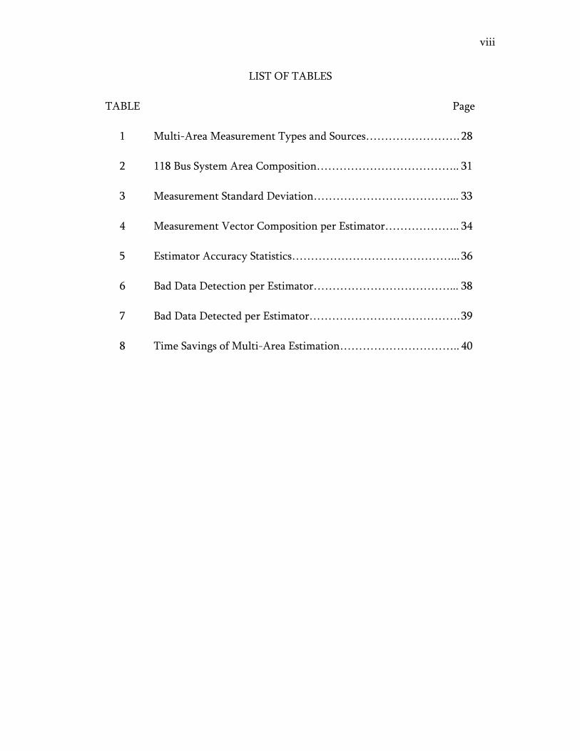
TABLE Page 1 Multi-Area Measurement Types and Sources……………………. 28

2 118 Bus System Area Composition……………………………….. 31 3 Measurement Standard Deviation………………………………... 33 4 Measurement Vector Composition per Estimator……………….. 34 5 Estimator Accuracy Statistics……………………………………... 36 6 Bad Data Detection per Estimator………………………………... 38 7 Bad Data Detected per Estimator…………………………………. 39 8 Time Savings of Multi-Area Estimation………………………….. 40

1

CHAPTER I

INTRODUCTION

1.1 Modern Power Systems

The society that we live in depends on electricity. Electricity allows for instant

communication across the globe, climatizes our buildings, and has let us extend our

life span by more than 40 years [1]. It is the job of the power system engineers to

ensure that this electricity is ready and available whenever it is required. These

engineers have many tools at their disposal, and use everything from load forecasting

to state estimation to ensure there is power at the flick of a switch.

Recently though, the power grid has become deregulated. In place of a large block of

generators, transformers, and transmission lines owned and operated by a single

company, there exists now a slapdash amalgamation of smaller companies each filling

their own niche. This segmentation of the power grid has made the power system

engineer’s job much more complex. To complete the state estimation of the power

grid, information must be gathered from many smaller, and often competing,

companies. These companies may also utilize different algorithms and standards for

their state estimators, and may feel reluctant to share this information with their

competitors. These facts coupled with the massive size of the modern power system

________________________ This thesis follows the style and format of IEEE Transactions on Power Systems.

2

has made time efficient, numerically accurate state estimation difficult.

1.2 Multi-Area State EstimationA new trend power system state estimation has emerged to combat these difficulties.

This new approach, known as parallel or multi-area state estimation, involves

breaking the problem down into two steps. The first step produces only the solution

for subsystems, or individual areas, within the power grid. Once complete, the data

from the individual areas feeds into the second step to create a single coordinated

solution for the entire power system. This multi-area approach has been addressed in

[2]-[3].

This thesis will demonstrate by example and simulation such an approach when

applied to a sample power system. The IEEE 118 Bus Test System, divided into five

different areas, shall serve as the sample system. The results produced by the multi-

area state estimator will be compared with those of a standard single level, or serial

state estimator and checked for accuracy, bad data detection, and time savings.

The particular algorithm used in this thesis was developed in [4]. In addition to

conventional measurements such as bus power injections, line power flows, bus

voltage and line current magnitudes, it also relies on the use of synchronized phasor

measurement units (PMUs). These measurements allow for both the magnitude as

well as the phase angle of bus voltages to be observed synchronized in time via the

3

Global Positioning System (GPS) technology. In this thesis, we will consider the use

of few PMUs as measurement devices in different areas in order to facilitate

synchronization of area slack bus voltage estimates.

1.3 Thesis Contribution

The contribution of this thesis will primarily be the application of a multi-area state

estimation algorithm to sample power system. The multi-area technique will be

explained and demonstrated on the IEEE 118 bus test system.

1.4 Thesis Organization

This thesis is organized into five chapters. In Chapter I, the current state of state

estimation will be presented along with its challenges and some proposed solutions.

Chapter II will deal with the nature of the state estimation problem and an algorithm

will be developed taking into account the types of measurements, conventional or

PMU, the issues involved with bad data and observability, and issues which appear

with a multi-area approach. Chapter III will go deeper into the multi area solution

and an algorithm will be developed and will address the issues raised in Chapter II.

Chapter IV will present the results of this algorithm when applied to the IEEE sample

system. Chapter V will summarize this thesis and point out work that still needs to be

done in this field.

4

CHAPTER II

SERIAL STATE ESTIMATION

2.1 Weighted Least Squares Estimation

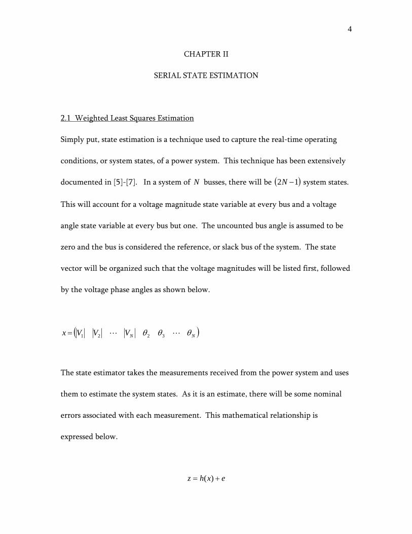
Simply put, state estimation is a technique used to capture the real-time operating

conditions, or system states, of a power system. This technique has been extensively

documented in [5]-[7]. In a system of busses, there will be ( )12 −NN system states.

This will account for a voltage magnitude state variable at every bus and a voltage

angle state variable at every bus but one. The uncounted bus angle is assumed to be

zero and the bus is considered the reference, or slack bus of the system. The state

vector will be organized such that the voltage magnitudes will be listed first, followed

by the voltage phase angles as shown below.

( )NNVVVx θθθ LL 3221=

The state estimator takes the measurements received from the power system and uses

them to estimate the system states. As it is an estimate, there will be some nominal

errors associated with each measurement. This mathematical relationship is

expressed below.

exhz += )(

5

( )( )

( ) ⎥⎥⎥⎥

⎦

⎤

⎢⎢⎢⎢

⎣

⎡

+

⎥⎥⎥⎥

⎦

⎤

⎢⎢⎢⎢

⎣

⎡

=

⎥⎥⎥⎥

⎦

⎤

⎢⎢⎢⎢

⎣

⎡

mnn

n

n

m e

ee

xxxh

xxxhxxxh

z

zz

M

L

M

L

L

M2

1

21

212

211

2

1

,,,

,,,,,,

is the measurement vector [ mT zzzz ,,, 21 L= ]

]( ) ( ) ( )[ xhxhxhh nT ,,, 21 L= is the non-linear function relating the states to

the measurements

is the measurement error vector [ ]mT eeee ,,, 21 L=

The errors are assumed to be independent and uncorrelated with a zero mean.

Furthermore, they are assumed to have a Gaussian (Normal) distribution. The

covariance matrix associated with the errors will be a diagonal matrix R with the

variance of the measurements as its entries.

{ } mieE i ,,2,10 L==

{ } jimjmieeE ji ≠=== ,,2,1,,2,10 LL

( ) { } { }222

21 ,,, m

T diagReeEeCov σσσ L==⋅=

In this thesis, weighted least squares (WLS) estimation will be applied to the above

equations in order to extract the state quantities, bus voltages and angles, from the

6

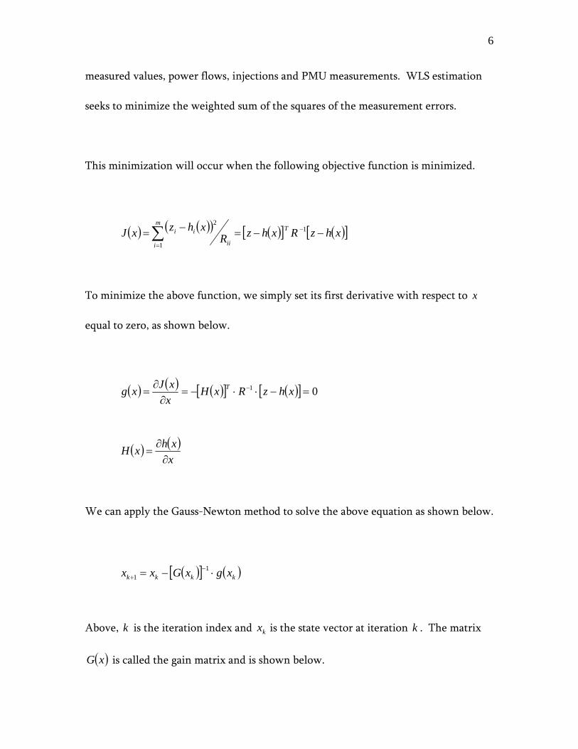
measured values, power flows, injections and PMU measurements. WLS estimation

seeks to minimize the weighted sum of the squares of the measurement errors.

This minimization will occur when the following objective function is minimized.

( ) ( )( ) ( )[ ] ( )[ ]∑=

− −−=−=m

i

T

ii

ii xhzRxhzRxhzxJ

1

12

To minimize the above function, we simply set its first derivative with respect to x

equal to zero, as shown below.

( ) ( ) ( )[ ] ( )[ ] 01 =−⋅⋅−=∂

∂= − xhzRxH

xxJxg T

( ) ( )xxhxH

∂∂

=

We can apply the Gauss-Newton method to solve the above equation as shown below.

( )[ ] ( )kkkk xgxGxx ⋅−= −+

11

Above, is the iteration index and kxk is the state vector at iteration . The matrix

is called the gain matrix and is shown below.

k

( )xG

7

( ) ( ) ( )[ ] ( )kT

kk

k xHRxHxxgxG ⋅⋅=

∂∂

= −1

( ) ( )[ ] ( )[ ]kT

kk xhzRxHxg −⋅⋅−= −1

The gain matrix is typically rather sparse and decomposed into its triangular factors.

For every iteration, forward and backward substitutions are used to solve the

following linear equations.

( )[ ] ( )[ ] ( )[ ] ( )[ ] kT

kkT

kk zRxHxhzRxHxxG Δ⋅⋅=−⋅⋅=Δ −−+

111

kkk xxx −=Δ ++ 11

These iterations will continue until one of two conditions are met. The first

condition would be the maximum number of allowable iterations is exceeded while

the second condition would be that the change in state variables has fallen within an

acceptable range.

ε<Δ kxmax

8

A popular initial condition for state estimation is the flat start. This condition sets the

voltages of all the busses equal to 1 p.u. with no phase change among the busses.

2.2 Treatment of Conventional Measurements

The five types of conventional measurements used in power system state estimation

are real and reactive line power flows, real and reactive bus power injections, and the

bus voltage magnitudes. In order to use these measurements in the state estimator,

we must first develop a mathematical model for the measurements. To do this,

consider the pi model of a transmission line which connects two busses i and , as

shown in Figure 1. The series admittance between bus i and will be defined as

j

j

ijij jbg + while the shunt admittance between any particular bus x and the ground

will be defined as . The admittance matrix Y will be composed of

entries, with the entry

sxsx jbg + ji ⋅

ijijij jBGY += .

iBus jBusijg ijb

sjsj jbg +sisi jbg +

Figure 1. Conventional Measurement Transmission Line Model

9

Developing the equations for the power injection at bus i yields:

( )∑∈

+=N

Njijijijijjii

i

BGVVP θθ sincos

( )∑∈

−=N

Njijijijijjii

i

BGVVQ θθ cossin

For a real power injection, the Jacobian matrix components are shown below.

( )∑=

−+=∂∂ N

jiiiijijijijj

i

i GVBGVVP

1

2sincos θθ

( )ijijijijij

i BGVVP θθ sincos +=

∂∂

( )∑=

−+−=∂∂ N

jiiiijijijijji

i

i BVBGVVP1

2cossin θθθ

( )ijijijijjij

i BGVVP θθθ

cossin −=∂∂

10

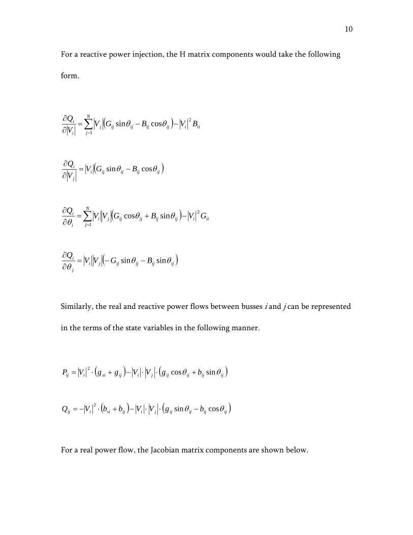
For a reactive power injection, the H matrix components would take the following

form.

( )∑=

−−=∂∂ N

jiiiijijijijj

i

i BVBGVVQ

1

2cossin θθ

( )ijijijijij

i BGVVQ θθ cossin −=

∂∂

( )∑=

−+=∂∂ N

jiiiijijijijji

i

i GVBGVVQ1

2sincos θθθ

( )ijijijijjij

i BGVVQθθ

θsinsin −−=

∂∂

Similarly, the real and reactive power flows between busses i and j can be represented

in the terms of the state variables in the following manner.

( ) ( )ijijijijjiijsiiij bgVVggVP θθ sincos2 +⋅⋅−+⋅=

( ) ( )ijijijijjiijsiiij bgVVbbVQ θθ cossin2 −⋅⋅−+⋅−=

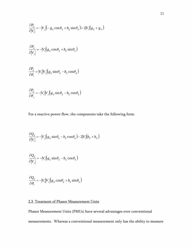
For a real power flow, the Jacobian matrix components are shown below.

11

( ) ( )siijiijijijijji

ij ggVbgVVP

+++−−=∂

∂2sincos θθ

( )ijijijijij

ij bgVVP

θθ sincos +−=∂

∂

( )ijijijijjii

ij bgVVP

θθθ

cossin −=∂

∂

( )ijijijijjij

ij bgVVP

θθθ

cossin −−=∂

∂

For a reactive power flow, the components take the following form.

( ) ( )siijiijijijijji

ij bbVbgVVQ

+−−−=∂

∂2cossin θθ

( )ijijijijij

ij bgVVQ

θθ cossin −−=∂

∂

( )ijijijijjii

ij bgVVQ

θθθ

sincos +−=∂

∂

2.3 Treatment of Phasor Measurement Units

Phasor Measurement Units (PMUs) have several advantages over conventional

measurements. Whereas a conventional measurement only has the ability to measure

12

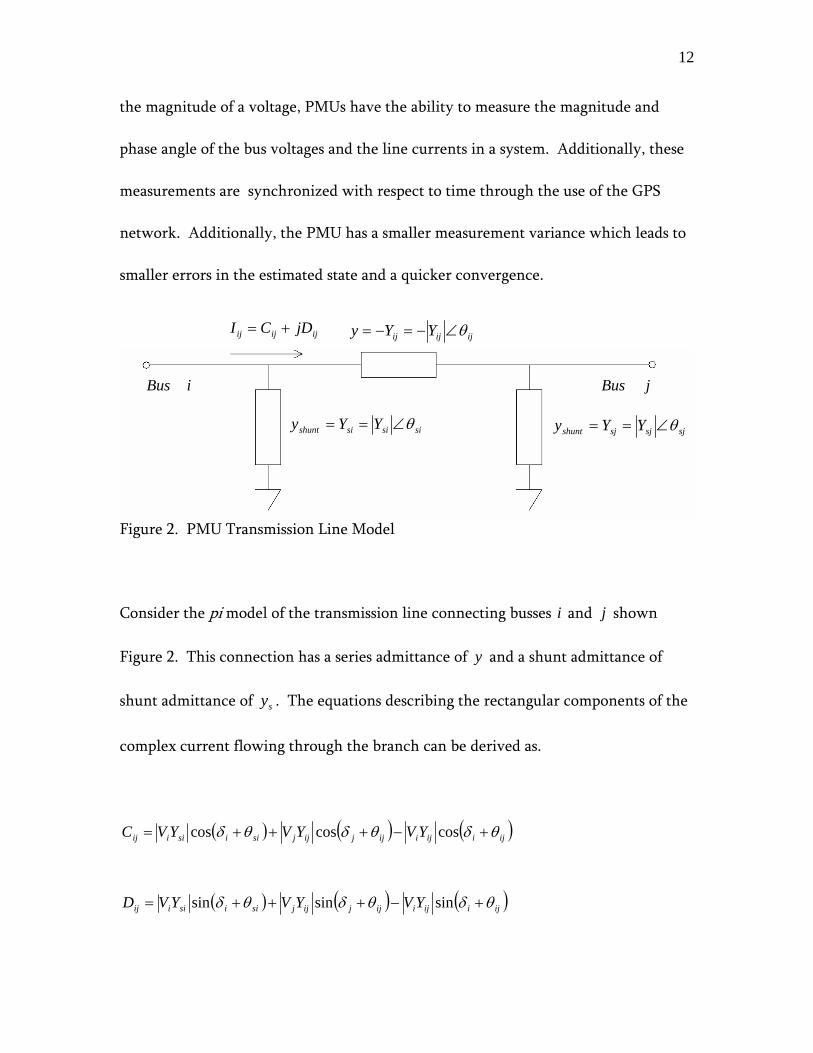
the magnitude of a voltage, PMUs have the ability to measure the magnitude and

phase angle of the bus voltages and the line currents in a system. Additionally, these

measurements are synchronized with respect to time through the use of the GPS

network. Additionally, the PMU has a smaller measurement variance which leads to

smaller errors in the estimated state and a quicker convergence.

ijijij jDCI +=

ijijij YYy θ∠−=−=

iBus jBus

sisisishunt YYy θ∠== sjsjsjshunt YYy θ∠==

Figure 2. PMU Transmission Line Model

Consider the pi model of the transmission line connecting busses i and shown

Figure 2. This connection has a series admittance of and a shunt admittance of

shunt admittance of . The equations describing the rectangular components of the

complex current flowing through the branch can be derived as.

j

y

sy

( ) ( ) ( )ijiijiijjijjsiisiiij YVYVYVC θδθδθδ +−+++= coscoscos

( ) ( ) ( )ijiijiijjijjsiisiiij YVYVYVD θδθδθδ +−+++= sinsinsin

13

When the Jacobian H matrix is formed, the following derivatives of Cij and Dij are

used.

( ) ( )ijiijsiisii

ij YYVC

θδθδ +−+=∂

∂coscos

( )ijjijj

ij YVC

θδ +=∂

∂cos

( ) ( )ijiijisiisiii

ij YVYVC

θδθδδ

+++−=∂

∂sinsin

( )ijjijjj

ij YVC

θδδ

+−=∂

∂sin

( ) ( )ijiijsiisii

ij YYVD

θδθδ +−+=∂

∂sinsin

( )ijjijj

ij YVD

θδ +=∂

∂sin

( ) ( )ijiijisiisiii

ij YVYVD

θδθδδ

+−+=∂

∂cossin

( )ijjijjj

ij YVD

θδδ

+=∂

∂cos

14

When we employ PMUs in a power system, the measurement vector is augmented.

Instead of containing only the voltage magnitude, power flows, and power injections

provided by conventional measurements, it will also include the phase shifts and the

real and reactive current flows throughout the system. The augmented measurement

vector will take on the following form.

( )TTij

Tij

TTTflo

Tflo

Tinj

Tinj DCVQPQPz δ=

2.4 Bad Data Processing

State estimators of all varieties are susceptible to the problem of bad data corruption.

This bad data can come from many sources including a malfunctioning measurement

device, a noisy communication channel, or even a failure in the communication

channel. Whatever the source of the bad data, it will serve to bias the state estimator,

causing it to return inaccurate results. One way of detecting the presence of bad data

is using the test. This test looks at the measurement vector in an effort to

determine the presence of faulty data. A second test involves the inspection of the

normalized residuals to determine specifically which measurement is malfunctioning.

2χ z

15

The test may be looked at as having three separate steps. First, the state estimator

must be run in order to obtain an estimate of the power systems state, . Once this

state estimate has been calculated, the system’s objective function must be developed.

The objective function is of the following form.

2χ

x

( ) ( )( ) ∑∑=

−

=

=⎟⎟⎠

⎞⎜⎜⎝

⎛ −=

m

iiii

m

i ii

ii eRR

xhzxJ1

21

1

2

At this point, we can assume that all the error terms, , will be random variables

which are independent and approximately normally distributed in the following

manner.

ie

( )( ) ( )iiiii RNxhze ,0~ˆ−=

Now we are able to normalize the errors and obtain a new function . ( )xu

( )ii

iii R

xhzu −=

( )xuOnce we have formulated the function , we enter the third part of the test. Now

we must compute the test statistic with ( )nm −2χ degrees of freedom, where is m

16

the total number of measurements in the system and is the number of states of the

system. The false alarm rate

n

α is then selected and a table is consulted. If the

value of the objective function

2χ

( )xJ ˆ is greater than the value, then we should

suspect to have at least one piece of bad data in our measurement set. Should the

value of the objective function be less than the value, this is a good indication that

all measurements are functioning properly.

2χ

2χ

There are two main shortcomings of this test. First of all, this is a cumulative test.

This means that some of the outlying data points may be lost in the average, making

this test less than perfect. Secondly, this test simply indicates the presence of bad data

in our measurement set. The test does not have the ability to single out the

individual pieces of offending data, but merely says that they exist.

2χ

In order to find which specific measurement is incorrect, we must rely on another

algorithm. This thesis will employ normalized residual testing in order to find the

problematic measurements. In this technique, inspection of the normalized values of

the residuals will point out which measurement is bad.

In order to use normalized residual testing, we must first define a matrix called the

hat matrix, K .

17

11 −−= RHHGK T

zΔK zΔIt is known as the hat matrix because the multiplication of and results in ,

in other words, the hat matrix simply puts a hat on zΔ K. With this matrix, we are

now able to develop the residual sensitivity matrix, , in the following manner. S

zKzzzr Δ−Δ=Δ−Δ= ˆ

( )KIzr −Δ=

( )( exHKIr +Δ−= )

( )eKIxKHxHr −+Δ−Δ=

( ) SeeKIr =−=

RSince the covariance matrix for is assumed to be known as e , the above equation

can be used to derive the covariance matrix for the residual vector as follows: r

( )iii xhzr ˆ−=

( ) TSRSrVar =

18

It can be shown that is equal to by substituting with its expanded

definition and simplifying terms. Hence:

TSRS SR S

( ) iiiii SRrVar Ω==

( )iii Nr Ω,0~

We can normalize the residuals in the same manner that we normalized the errors to

produce . ( )xu

ii

iNi

rrΩ

=

( )1,0~ Nr Ni

Now that the residual values have been normalized, they may be compared to some

statistically reasonable value set by the observer based on the desired false alarm rate.

A threshold of 3.0 is used in this thesis. Any residuals exceeding this threshold are

suspect and should be treated.

The elimination of all bad data from a measurement set may be accomplished in the

following manner. Once the normalized residuals have been calculated, the largest

19

residual will correspond to the erroneous measurement. Instead of removing this

measurement from the vector, we are able to correct it using the following algorithm.

BADi

ii

iBADi

GOODi rZZ

Ω−=

2σ

( )BADi

BADi

BADi xHZr ˆ−=

In the above equations, and correspond to the corrected and initial,

suspect value of the normalized residual for measurement i . By replacing with

, the bad data treatment algorithm is complete for the largest normalized

residual of the group. The procedure may then be repeated until all normalized

residuals fall beneath the threshold set by the user.

GOODiZ BAD

iZ

BADiZ

GOODiZ

While this is a very useful technique for the discovery and elimination of bad data, it

too has its shortfalls. This test has problems if the measurement scheme of the system

is not robust. If there is a single piece of bad data, this algorithm will be unable to

correct it if the faulty data is from a critical measurement. A critical measurement is a

measurement which must be present in the system for the system to remain

observable.

20

When there are multiple pieces of bad data, there are two issues. The first issue is

concerned with the presence of a critical pair or k-tuple. These items are similar to

critical measurements in the fact that if all the component measurements are

removed, the system will become unobservable. There is also the issue of multiple

interacting errors. Conforming interacting errors in particular pose a problem for this

algorithm since it is possible for the conforming erroneous measurements to have

smaller residuals than the measurements which are indeed free of gross errors.

This chapter has looked into the basics of weighted least squares state estimation as

applied to electrical power systems. It has addressed the treatment of both

conventional measurements and PMUs and given two tests for the detection and

treatment of bad data. The next chapter will look at the process of multi-area state

estimation.

21

CHAPTER III

MULTI-AREA STATE ESTIMATION

3.1 Introduction

As the electrical power networks of the world continue to grow ever larger, there has

been an increasing demand for a highly robust, computationally efficient state

estimation algorithm. Initially, this goal was pursued by taking advantage of the

innately sparse structure of the state estimation matrices. New algorithms were

developed to deal with large, sparse matrices and the state estimators kept pace with

the power grids for a time. Unfortunately, the gains provided by sparse matrix

manipulation were limited, and eventually the size of the power networks required a

new advance in state estimation algorithms.

This new advance came in the form of parallel processing. Instead of being limited to

a single serial processor, the parallel state estimators break the large system down into

smaller sub-systems which are solved simultaneously on multiple processors. The

state estimation results from these individual areas are then sent to a second

coordinating processor where they are combined into a single solution for the entire

system.

22

3.2 Multi-Area State Estimation

In any individual area in multi-area state estimation, there are three types of busses:

internal, boundary, and external. Bus of area is considered to be internal if all of

its neighboring busses also belong to area . Bus of area i is a boundary bus if at

least one of its neighbors belongs to an area other than i . Finally, bus will be an

external bus of area if it belongs to another area but has at least one connection to a

boundary bus in area i . Any line running between two boundary busses of different

areas, thus connecting the two areas, is known as a tie line. These four items are

illustrated in the Figure 3 with busses 21, 22, and 23 being internal, boundary, and

external busses to Area 1. There is a tie line running between busses 22 and 23 and

another between 32 and 113.

in

i n

n

i

Figure 3. Multi-Area Bus Types

Since its inception, there have been many specific algorithms developed to carry out

this parallel state estimation, some of the more successful ones have been detailed in

[8]-[13]. In most cases, the first level state estimation is identical. The large system is

23

broken down into smaller, more manageable areas and the standard state estimation

algorithm is applied, as was shown in Chapter II. There is a great deal of confusion

though about what to do from that point. Most of this confusion concerns what to do

with the boundary measurements. Some algorithms insert a non-existent bus in

between the boundary busses on tie lines [14]. Other methods based on the work in

[15] break the system down into non-overlapping systems and then apply the model

coordination method to come to a solution. More recently though, the work done in

[4] and [16] has developed the algorithm which will be used in this thesis.

In [16] the author first decomposes the system into a group of overlapping

subsystems. This is accomplished by including the boundary busses and external

busses in both areas which they are associated with. Once the first stage of state

estimation is complete, the state vectors for each area are organized in the following

manner.

[ ]TTT extii

bii xxxx int=

For each area , the components of the state vector are organized by bus type. In

the equation above, is the state vector composed of the voltage magnitude and

phase angles at the boundary busses, is the state vector composed of the voltage

ixi

Tbix

T

ixint

24

magnitude and phase angles at the internal busses, and is the state vector

composed of the voltage magnitude and phase angles at the external busses. In each

area, the phase angle of the slack bus will be removed from the appropriate vector.

Textix

Once this first stage is complete, the estimation coordination must begin. The

coordinating estimator is not only responsible for the coordinating of the individual

area results, but must also carry out bad data detection and correction for the

boundary measurements. The states used in this coordinating estimator include not

only the states computed for each individual area, but also include the synchronized

voltage phasors for the slack bus in each area. This state vector is defined in the

following manner.

[ ]TTbs uxx

T

=

[ ]Tbn

bbb TTTT

xxxx L21=

[ ]TnT uuuu L32=

The voltage angle of the slack bus in each area measured with respect to the voltage

angle of the slack bus in the first area is listed as . The global reference bus among

the individual area slack busses was chosen at random to be the slack bus in the first

iu

25

area, and could easily be any of the slack busses in the system. In this case, the

vector would start with and exclude the appropriate entry containing the slack

reference bus.

Tu

1u

At the second level of state estimation, the coordinating estimator will utilize a

measurement vector with the following composition.

[ ]TextbTsp

Tu

TT

xxzzz ˆˆ=

In the above measurement vector, is the vector of boundary measurements, is

the vector of synchronized phasor measurements, and and are the vectors of

boundary and external state variables as estimated by the individual areas. This

vector of states will then be treated as pseudo-measurements by the coordinating

estimator. This leads us to the measurement model which will be used by the second

level state estimator shown below.

TspzT

uz

TbxTextx

( ) ssss exhz +=

26

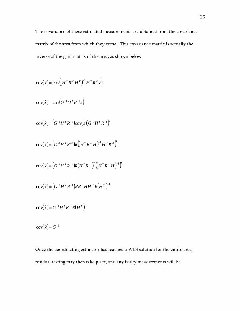
The covariance of these estimated measurements are obtained from the covariance

matrix of the area from which they come. This covariance matrix is actually the

inverse of the gain matrix of the area, as shown below.

( ) ( )( )zRHHRHx TTT 111covˆcov −−−=

( ) ( )zRHGx T 11covˆcov −−=

( ) ( ) ( )( )TTT RHGzRHGx 1111 covˆcov −−−−=

( ) ( ) ( )( )TTTT RHHRHRRHGx 11111ˆcov −−−−−=

( ) ( ) ( ) ( )( )TTTTT HRHRHRRHGx 11111ˆcov −−−−−=

( ) ( ) ( ) 11111ˆcov −−−−−= TT HRHHRRRHGx

( ) ( ) 111ˆcov −−−= TT HRRHGx

( ) 1ˆcov −=Gx

Once the coordinating estimator has reached a WLS solution for the entire area,

residual testing may then take place, and any faulty measurements will be

27

normalized. While this is an excellent procedure since it does not require the sharing

of data between the areas, it can be improved upon still.

In [4], the author points out that the above technique simply uses the PMUs to

measure the synchronized voltage angles among the areas and suggests the following.

PMUs have the ability to measure the real and reactive current phasors. In fact, a

single PMU may measure a bus voltage phasor and multiple current phasors

simultaneously. As the measurements taken from PMUs have smaller variance than

conventional measurements, the estimated state would benefit from the inclusion of

these additional PMU current measurements.

The first level of state estimation with PMUs would follow the algorithm outlined in

Chapter II. Once the states of the individual areas have been estimated though, the

second level algorithm needs to be changed in order to accommodate the additional

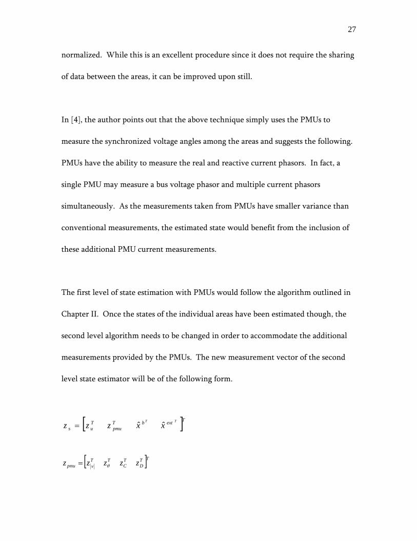
measurements provided by the PMUs. The new measurement vector of the second

level state estimator will be of the following form.

[ ]TextbTpmu

Tus

TT

xxzzz ˆˆ=

[ ]TTD

TC

TTvpmu zzzzz θ=

28

[ ]TextbTD

TC

TTv

Tus

TT

xxzzzzzz ˆˆθ=

Above, is the measurement vector from a PMU. The overall measurement

vector, , will contain twelve different types of measurements, four from

conventional measurements, four from PMU measurements, and four pseudo-

measurements from the first level of estimation. These twelve measurement types are

detailed below.

PMUz

sz

Table 1. Multi-Area Measurement Types and Sources

Source Measurement

Real power flow

Reactive power flow

Real power injection Conventional

Reactive power injection

Voltage magnitude

Voltage phase angle

Real Current PMU

Reactive Current

Boundary bus voltage magnitude

Boundary bus voltage phase angle

External bus voltage magnitude Estimated

External bus voltage phase angle

29

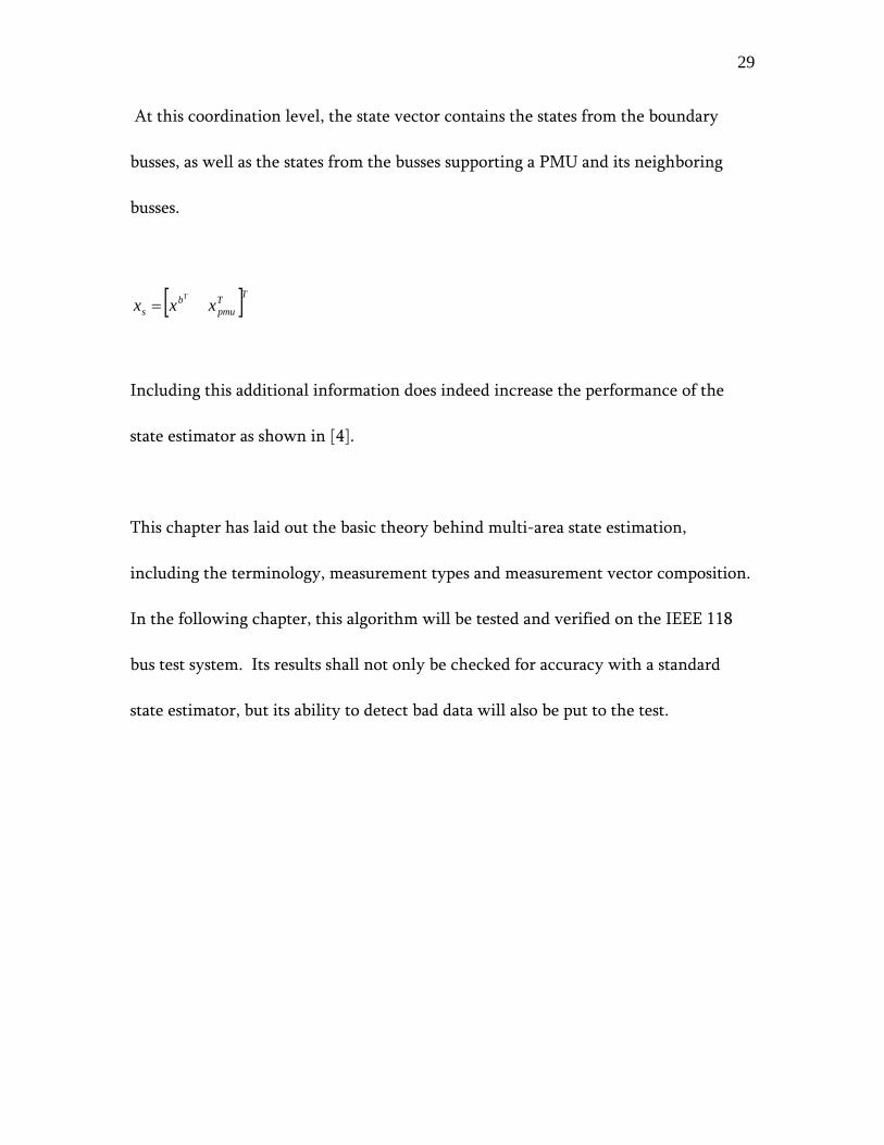
At this coordination level, the state vector contains the states from the boundary

busses, as well as the states from the busses supporting a PMU and its neighboring

busses.

[ ]TTpmu

bs xxx

T

=

Including this additional information does indeed increase the performance of the

state estimator as shown in [4].

This chapter has laid out the basic theory behind multi-area state estimation,

including the terminology, measurement types and measurement vector composition.

In the following chapter, this algorithm will be tested and verified on the IEEE 118

bus test system. Its results shall not only be checked for accuracy with a standard

state estimator, but its ability to detect bad data will also be put to the test.

30

CHAPTER IV

SIMULATION RESULTS

4.1 118 Bus Area Geography

Before the test system is fed into the estimator, it must first be broken down into

individual areas. The division of these areas do not play an important role in the

second level solution, so the formation of the areas is subject to only one stipulation,

the individual areas must be observable. If an individual area is unobservable, the

first level state estimator will be unable to converge for that area. This will lead to

missing information for the second level estimator, again causing a non-converging

error. I chose to break the system down into five areas. Table 2 details the bus

composition of each area in the IEEE 118 bus test system. Figure 4 shows the IEEE

118 Bus Test System. In the system diagram, the slack busses for each area are shown

in blue. The arrows branching off of the slack busses indicate a complex current

measurement, provided by the PMU at that bus.

31

Table 2. 118 Bus System Area Composition

Area 1 2 3 4 5

Internal Busses 20 16 22 14 4

Boundary Busses 6 11 5 11 9

External Busses 7 9 6 10 13

Total Busses 26 27 27 25 13

Slack Bus No. 3 27 103 35 47

32

Figu

re 4

. IE

EE 1

18 B

us T

est S

yste

m

33

4.2 Measurement Vector Composition In order to create the measurements used by the state estimators in this thesis, a

power flow analysis was first run on the integrated system. The resulting currents

and power flows were then perturbed by a small amount to simulate the variance

found in actual measurements. The different types of measurements were subjected

to different amounts of perturbation, as detailed in Table 3. Notice that the standard

deviation of all the PMU measurements is significantly smaller than the standard

deviation of the conventional measurements. This reflects the increased precision of

the newer PMUs over the conventional measurement devices.

Table 3. Measurement Standard Deviation

Measurement Type Standard Deviation

Conventional Power Injection 0.01

Conventional Power Flow 0.008

PMU Real Current 0.000001

PMU Reactive Current 0.000001

PMU Voltage Magnitude 0.000001

PMU Voltage Angle 0.000001

In the serial estimator and the individual area estimators, the boundary busses

received a real and reactive power injection measurement pair. All branches received

at least one real and reactive power flow measurement pair, and if the branch was

associated with a boundary bus, it received a second real and reactive power flow

34

measurement pair. Finally, the slack busses in each area received a PMU voltage

magnitude measurement.

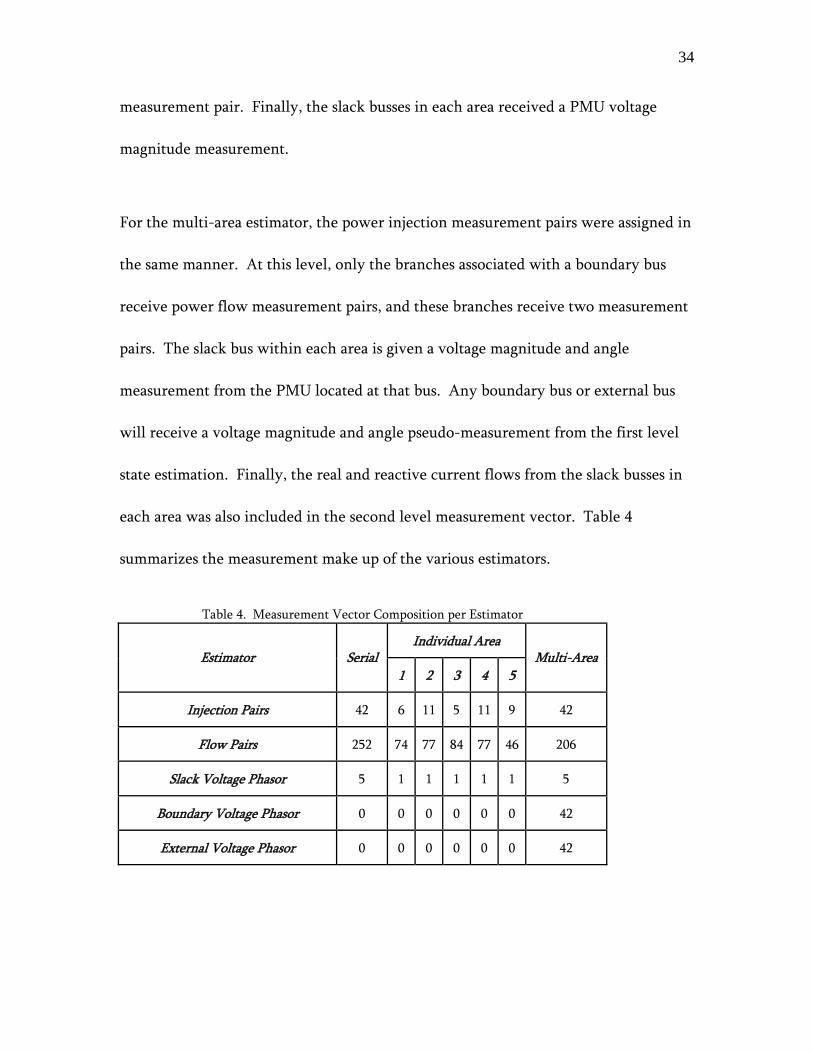
For the multi-area estimator, the power injection measurement pairs were assigned in

the same manner. At this level, only the branches associated with a boundary bus

receive power flow measurement pairs, and these branches receive two measurement

pairs. The slack bus within each area is given a voltage magnitude and angle

measurement from the PMU located at that bus. Any boundary bus or external bus

will receive a voltage magnitude and angle pseudo-measurement from the first level

state estimation. Finally, the real and reactive current flows from the slack busses in

each area was also included in the second level measurement vector. Table 4

summarizes the measurement make up of the various estimators.

Table 4. Measurement Vector Composition per Estimator

Individual Area Estimator

Serial

1 2 3 4 5Multi-Area

Injection Pairs 42 6 11 5 11 9 42

Flow Pairs 252 74 77 84 77 46 206

Slack Voltage Phasor 5 1 1 1 1 1 5

Boundary Voltage Phasor 0 0 0 0 0 0 42

External Voltage Phasor 0 0 0 0 0 0 42

35

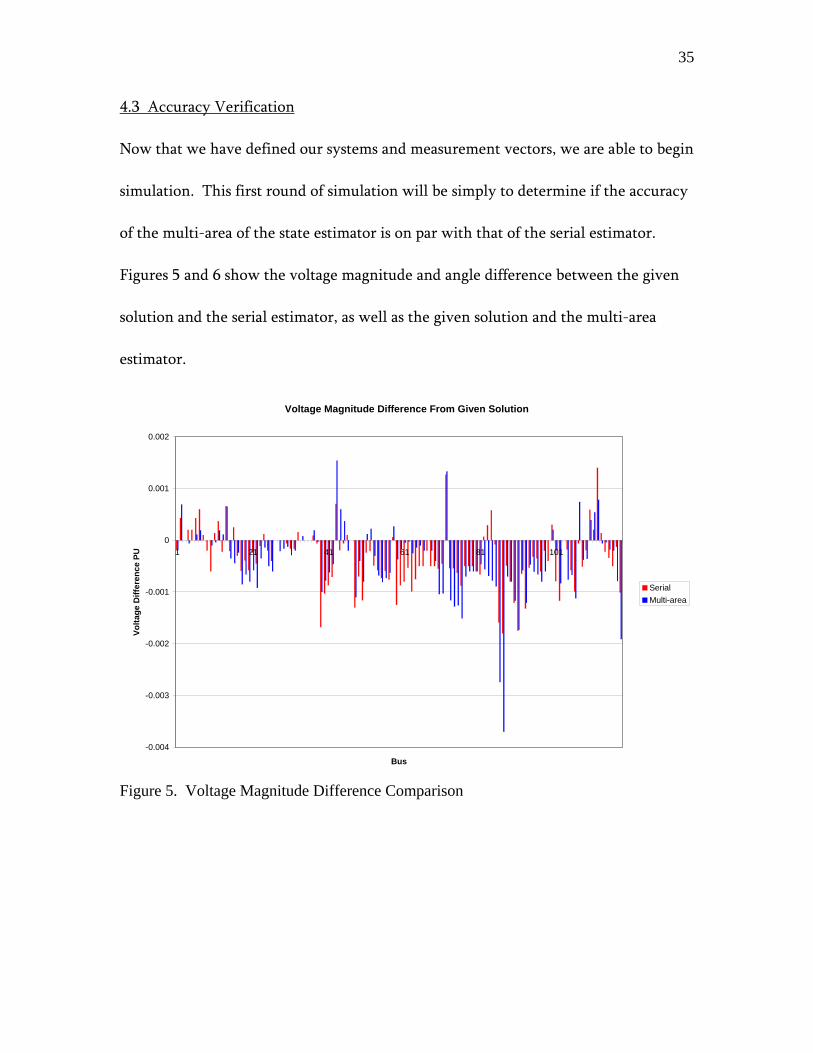
4.3 Accuracy Verification

Now that we have defined our systems and measurement vectors, we are able to begin

simulation. This first round of simulation will be simply to determine if the accuracy

of the multi-area of the state estimator is on par with that of the serial estimator.

Figures 5 and 6 show the voltage magnitude and angle difference between the given

solution and the serial estimator, as well as the given solution and the multi-area

estimator.

Voltage Magnitude Difference From Given Solution

-0.004

-0.003

-0.002

-0.001

0

0.001

0.002

1 21 41 61 81 101

Bus

Volta

ge D

iffer

ence

PU

SerialMulti-area

Figure 5. Voltage Magnitude Difference Comparison

36

Phase Angle Difference from Given Solution

-0.2

-0.15

-0.1

-0.05

0

0.05

0.1

0.15

0.2

0.25

1 21 41 61 81 101

Bus

Ang

le D

iffer

ence

(deg

rees

)

SerialMulti-area

Figure 6. Phase Angle Difference Comparison

While Figures 5 and 6 may be a little confusing, their pertinent statistics are

summarized in the Table 5 below.

Table 5. Estimator Accuracy Statistics

Estimator Serial Estimator Multi-Area Estimator

Mean Voltage Difference -0.00033 -0.00038

Mean Angle Difference (°) 0.00004 -0.00362

Voltage Difference Standard Deviation 0.00055 0.00067

Angle Difference Standard Deviation (°) 0.04909 0.04318

Max Voltage Difference 0.0018 0.0037

Max Angle Difference (°) 0.22286 0.13645

37

It can be seen that the difference between the serial estimator and the multi-state

estimator is minimal. This verifies that the multi-state estimator does function

correctly given ideal conditions. The next step is to verify the multi-state estimator’s

ability to detect bad data.

4.4 Bad Data Detection

As pointed out in Chapter II, the state estimators use a test to detect the presence

of bad data and then an investigation of the normalized residual values will point out

the specific measurement which is returning the bad data.

2χ

For the test, the objective function of the system must be compared to a threshold

value. This value is determined by setting a false alarm probability,

2χ

α and the

degrees of freedom for the system, given by ( )( )12 −− Nm , where is the total

number of measurements in the area and is the number of busses in the area.

When the value of any normalized residual exceeds 3.0, this indicates the

measurement associated with that residual is returning bad data. Table 6 lays out the

data and thresholds used for bad data detection with for the serial, individual area,

and multi-area state estimators.

m

N

38

Table 6. Bad Data Detection per Estimator

Individual Area Estimator

Multi-Area Serial

1 2 3 4 5

Measurements 593 161 177 179 177 111 680

Busses 118 26 27 27 25 13 118

Degrees of Freedom 356 108 122 124 126 84 443

False Alarm Rate 0.01 0.01 0.01 0.01 0.01 0.01 0.01

Chi-squared Value 421.00 145.10 161.25 163.55 165.84 117.06 515.17

Objective Function 348.43 93.22 105.99 112.17 126.08 57.41 481.69

Largest Normalized Residual 0.301 0.278 0.242 0.250 0.281 0.276 0.403

As can be seen above, the largest normalized residuals for each of the estimators is

well below the 3.0 threshold, indicating all the data is within reason. This fact is

further confirmed since the objective function of each of the areas is well below the

chi-squared value as determined by the degrees of freedom and the false alarm rate.

To test the multi-area estimator’s ability to detect bad data, let us force a bad power

injection measurement at Bus 19 in Area 1. By changing the computed measurement

value from -0.46304 to -1, we will be able to see if the estimators are able to first

detect and then isolate the bad data using both the and normalized residual tests. 2χ

39

Table 7 shows the results of this faulty measurement on the test statistics of the

system.

Table 7. Bad Data Detected per Estimator

Individual Area Estimator

Serial

1 2 3 4 5

Multi-Area

Chi-squared Value 421.00 145.10 161.25 163.55 165.84 117.06 515.17

Objective Function 1575.90 1233.20 126.38 109.30 98.92 48.62 1935.50

Largest Normalized Residual 3.512 3.381 0.295 0.275 0.312 0.253 3.650

It can be seen that the multi-area estimator does indeed have the ability to detect bad

data. This is evident in the fact that the objective function of the system is greater

than the chi-squared test statistic. The only measurement residual which was larger

than the allowed threshold of 3.0 was the residual which corresponded to the power

injection measurement at Bus 19.

4.5 CPU Time Savings

Now that this thesis has shown the multi-area state estimator to be accurate and

robust, we are able to examine the possible time savings which come from a parallel

processing scheme. The large scale of modern utility power systems were a driving

force behind the development of multi-area state estimators. Unfortunately, any time

savings seen on the IEEE 118 Bus Test System will be minimal at best due to its small

size, but the time savings will increase as the systems grow larger.

40

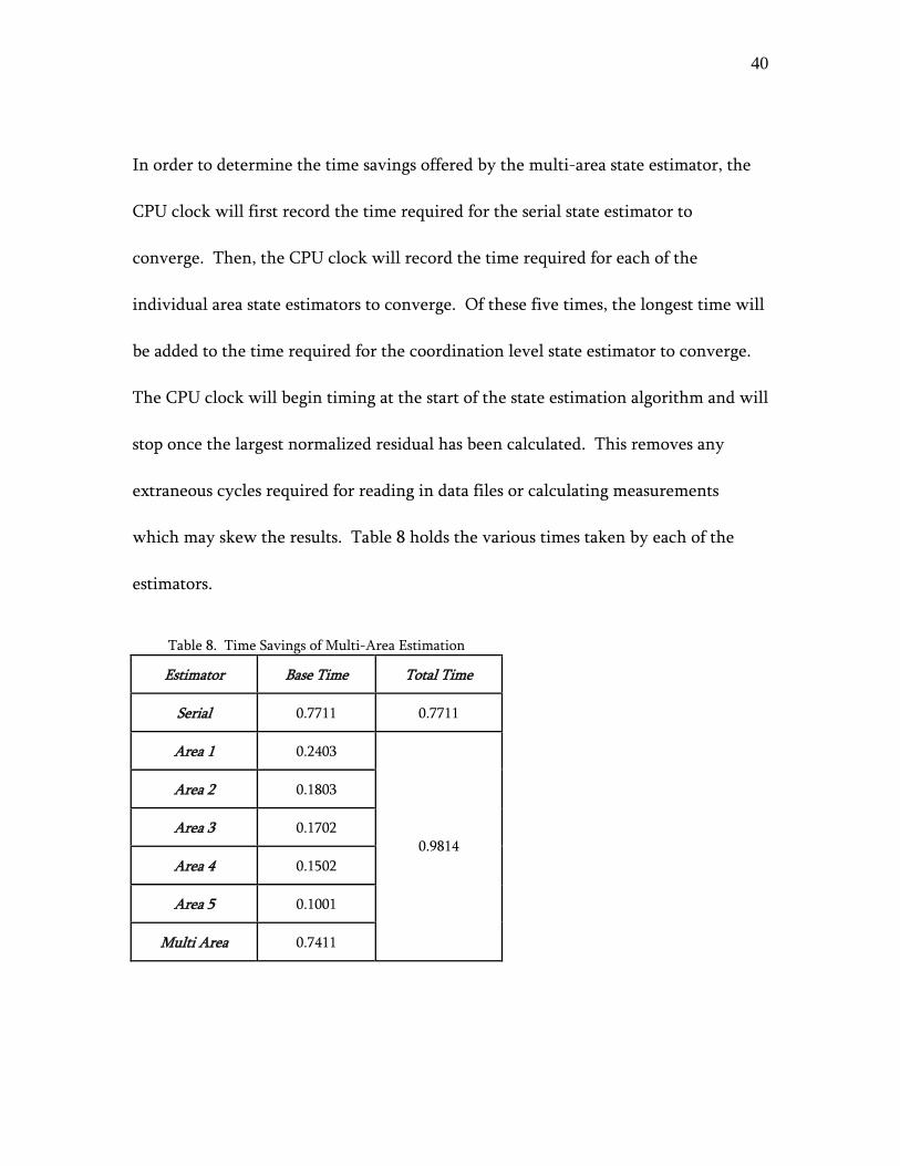
In order to determine the time savings offered by the multi-area state estimator, the

CPU clock will first record the time required for the serial state estimator to

converge. Then, the CPU clock will record the time required for each of the

individual area state estimators to converge. Of these five times, the longest time will

be added to the time required for the coordination level state estimator to converge.

The CPU clock will begin timing at the start of the state estimation algorithm and will

stop once the largest normalized residual has been calculated. This removes any

extraneous cycles required for reading in data files or calculating measurements

which may skew the results. Table 8 holds the various times taken by each of the

estimators.

Table 8. Time Savings of Multi-Area Estimation

Estimator Base Time Total Time

Serial 0.7711 0.7711

Area 1 0.2403

Area 2 0.1803

Area 3 0.1702

Area 4 0.1502

Area 5 0.1001

Multi Area 0.7411

0.9814

41

Unfortunately, on such a small scale the time savings of running a multi-area state

estimator are not apparent. When dealing with utility power systems which contain

thousands of busses and branches, one could expect a very real time savings.

This chapter has shown that the accuracy of the multi-area state estimator is on par

with that of a standard state estimator. The multi-area state estimator also is able to

use the same tests as a serial estimator to detect bad data received from its

measurements. Finally, an attempt was made to examine the time savings of multi-

area state estimation, but the scale of the system was too small for a determination to

be made.

42

CHAPTER V

CONCLUSION

5.1 Summary

Chapter II was a study in the theory of power system state estimation. The objective

of state estimation is to describe the real time operation of a power system in terms of

the systems states, bus voltage magnitude and phase angle. To do this, the state

estimator relies on various measurements taken from the power system, including

power injections, power flows, and PMU measurements. The power system

measurements were modeled as the sum of a non-linear function relating the error

measurements to the system states and a random variable representing error.

Weighted least squares estimation was then used to minimize the sum of the square of

the error. The mathematical equations related to the use of conventional and PMU

measurements in WLS estimation were derived and examined. Finally, the issue of

bad data processing was explored. There were two types of bad data treatments used

in this thesis. The chi-squared test was the first method and is only used to tell if

there is at least one bad measurement in the measurement vector. In order to

determine which specific measurement is bad, one needs to use the normalized

residual test.

43

Chapter III took the state estimation algorithm developed in Chapter II and attempted

to make it faster. To do this, the idea of a multi-area state estimator was discussed. In

a multi-area state estimator, the single large power system is broken down into

smaller areas. These individual areas each run their own state estimation algorithm

simultaneously and then pass the results to a second level coordinating estimator.

This second level estimation pieces the information from the first level to create a

single state vector for the entire system. The use of PMUs is vital at this coordination

level, and the use of their measurements was discussed.

Chapter IV was simply a verification of the validity of the multi-area state estimator

developed in Chapter III. In order to verify the accuracy of multi-area state

estimator, the IEEE 118 Bus Test System was first run through a serial state estimator.

This state vector and the state vector given as the solution were used as a baseline to

compare the performance of the multi-area state estimator. Then the IEEE 118 Bus

Test System was broken down into five areas in preparation for the multi-area state

estimator. The measurement scheme of the multi-area state estimator was once again

explained, and then the multi-area state vector was compared to the baseline. It was

shown that the performance of the multi-area state estimator was comparable to the

performance of the serial state estimator in terms of accuracy. The next test was to

see if the multi-area state estimator would be able to detect bad measurement data.

This was done by perturbing the measurement vector and in every case, the multi-

44

area state estimator detected the bad data with both the test and the normalized

residual test. Finally, the time savings stemming from the use of the multi-area state

estimator were investigated. Unfortunately, the size of the test system was such that

the gains were unobservable.

2χ

5.2 Future Work

While this thesis was successful in verifying the accuracy of the multi-area state

estimator, it was unable to see any time savings due to the implementation of said

estimator. It has been said many times throughout this thesis that the shortened

computation time was the impetus for the development of multi-area state estimation,

and as such, this deserves further study. The next logical step would be to increase

the size of the system and look for the promised reduction in computation time.

45

REFERENCES

[1] J. Oeppen, J.Vaupel, “Broken Limits to Life Expectancy,” SCIENCE, vol. 296,

pp. 1030-1031, May 2002.

[2] D.M. Falcao, F.F. Wu, L. Murphy, “Parallel and Distributed State Estimation,”

IEEE Transactions on Power Systems, vol. 10, no. 2, pp. 724-730, May 1995.

[3] J.B. Carvalho, F.M. Barbosa, “Parallel and Distributed Processing State

Estimation of Power System Energy,” 9th Mediterranean Electrotechnical

Conference, vol. 2, pp. 969-973, May 1998.

[4] Yeojun Yoon, “Study of the Utilization and Benefits of Phasor Measurement Units

for Large Scale Power System State Estimation,” MS Thesis, Texas A&M

University, Dec 2005.

[5] A. Bose, K.A. Clements, “Real-Time Modeling of Power Networks,” in Proc.

of the IEEE, vol. 75, no. 12, pp. 1607-1622, December 1987.

[6] A. Abur, A.G. Exposito, Power System State Estimation: Theory and

Implementation, New York, Marcel Dekker, 2004.

46

[7] F.C. Schweppe, J. Wildes, D.B. Rom, “Power System Static State Estimation I, II,

III,” IEEE Transactions on PAS, vol. PAS-89, no. 1, pp. 120-135, January 1970.

[8] D.P. Bertsekas, J.N. Tsitsikilis, Parallel and Distributed Computation, Upper

Saddle River, New Jersey, Prentice Hall, 1989.

[9] F.F. Wu, “Parallel Processing in Power Systems Computation,” IEEE Transactions

on Power Systems, vol. 7, no 2, pp. 629-638, August 1992.

[10] D.J. Tylavsky, A. Bose, F. Alvarado, R. Betancourt, K. Clements et al, “Parallel

Processing in Power Systems Computation,” IEEE Transactions on Power

Systems, vol. 7, no. 2, pp. 629-638, May 1992.

[11] K. Hwang, F. Briggs, Computer Architecture and Parallel Processing, New York,

McGraw-Hill, 1984.

[12] A.A. El-Keib, C.C. Carroll, H. Singh, D.J. Maratukulam, “Parallel State

Estimation in Power Systems,” Twenty-Second Southeastern Symposium on

System Theory, Cookeville, Tennessee, March 1990, pp. 255-260.

47

[13] T. Van Cutsem, M. Ribbens-Pavella, “Critical Survey of Hierarchical Methods

for State Estimation of Electric Power Systems,’ IEEE Transactions on PAS,

vol. PAS-102, no. 10, pp 3415-3424, October 1983.

[14] J.B. Carvalho, F.M. Barbosa, “A Parallel Algorithm to Power Systems State

Estimation,” 1998 International Conference on Power System Technology, vol.

2, pp. 1213-1217, August 1998.

[15] H. Kobayashi, S. Narita, M.S.A.A. Hammam, “Model Coordination Method

Applied to Power System Control and Estimation Problems,” in Proc. of the

IFAC/IFIP 4th International Conference, Santiago de Chile, 1974, pp. 291-298.

[16] L. Zhao, A. Abur, “Multi Area State Estimation Using Synchronized Phasor

Measurements,” IEEE Transactions on Power Systems, vol. 20, no. 2, pp. 611-

617, May 2005.

48

VITA

Name: Matthew Allan Freeman

Address: 560 22nd Street

Beaumont, TX 77706

Email Address: freeman.matt@gmail.com

Education: B.S., Electrical Engineering, Texas A&M University, 2004

M.S., Electrical Engineering, Texas A&M University, 2006