AachenDepartment of Computer Science

Technical Report

Solving Muller Games

via Safety Games

Daniel Neider, Roman Rabinovich, and Martin Zimmermann

ISSN 0935–3232 · Aachener Informatik-Berichte · AIB-2011-14

RWTH Aachen · Department of Computer Science · July 2011

The publications of the Department of Computer Science of RWTH AachenUniversity are in general accessible through the World Wide Web.

http://aib.informatik.rwth-aachen.de/

Solving Muller Games via Safety Games⋆

Daniel Neider1, Roman Rabinovich2, and Martin Zimmermann1

1 Lehrstuhl fur Informatik 7, RWTH Aachen University, Germany{neider,zimmermann}@automata.rwth-aachen.de

2 Mathematische Grundlagen der Informatik, RWTH Aachen University, Germanyrabinovich@logic.rwth-aachen.de

Abstract. We show how to transform a Muller game with n vertices into a safetygame with (n!)3 vertices whose solution allows to determine the winning regionsof the Muller game and a winning strategy for one player.

1 Introduction

Infinite two-player games are a powerful tool in the automated verification andsynthesis of non-terminating systems that have to interact with an antagonisticenvironment. There are also deep connections between infinite games and logicalformalisms like fixed-point logics or automata on infinite objects. In such a game,two players move a token through a finite graph, thereby constructing a playwhich is an infinite path. The winner is determined by a winning condition,which partitions the set of infinite paths in a graph into those that are winningfor Player 0 and those that are winning for Player 1. Typically, the winner of aplay is only determined after infinitely many steps.

Nevertheless, in some cases it is possible to give a criterion to define a finite-duration variant of an infinite game. Such a criterion stops a play after a finitenumber of steps and then declares a winner based on the finite play constructedthus far. It is called sound if Player 0 has a winning strategy for the infinite-duration game if and only if Player 0 has one for the finite-duration game.

It is easy to see that there is a sound criterion for positionally determinedgames: the players move the token through the arena until a vertex is visitedfor the second time. An infinite play can then be obtained by assuming that theplayers continue to play the loop that they have constructed, and the winner ofthe finite play is declared to be the winner of this infinite continuation.

For parity games (say, min-parity), Bernet, Janin, and Walukiewicz [1] gaveanother sound criterion based on the following observation: let nc be the numberof vertices with priority c. If a play visits nc + 1 vertices with odd priority cwithout visiting a smaller even priority in between, then the play has closeda loop which is losing for Player 0, assuming it is traversed from now on adinfinitum. However, no positional winning strategy can allow such a loop. Thus,Player 0 can prove that she has a winning strategy by allowing a play to visitan odd priority c at most nc times without seeing a smaller even priority inbetween. This condition can be turned into a safety game whose solution allowsto determine the winning regions of the parity game and a winning strategy forone of the players.

⋆ This work was supported by the projects Games for Analysis and Synthesis of InteractiveComputational Systems (GASICS) and Logic for Interaction (LINT) of the European ScienceFoundation.

In games that are not positionally determined, the situation gets more in-teresting since a player might have to pick different successors when a vertex isvisited several times. Therefore, the players have to play longer before the playcan be stopped and analyzed. Previous work considers Muller games which are ofthe form (A,F0,F1), where A is a finite arena and (F0,F1) is a partition of theset of loops in the arena. Player i wins a play if the set of vertices visited infinitelyoften is in Fi. Muller winning conditions are able to express all ω-regular winningconditions and subsume all other winning conditions that depend only on theinfinity set of a play (e.g., Buchi, co-Buchi, parity, Rabin, or Streett conditions).

To give a sound criterion for Muller games, McNaughton [7] defined for everyloop F ∈ F0∪F1 a scoring function ScF that keeps track of the number of timesthe set F was visited entirely (not necessarily in the same order) since the lastvisit of a vertex that is not in F . In an infinite play, the set of vertices seeninfinitely often is the unique set F such that ScF tends to infinity after beingreset to 0 only a finite number of times.

McNaughton proved the following criterion to be sound [7]: stop a play assoon as for some set F a score of |F |! + 1 is reached, and declare the winner tobe the Player i such that F ∈ Fi. However, it can take a large number of stepsfor a play to reach a score of |F |! + 1, as scores may increase slowly or be resetto 0. It can be shown that a play can be stopped by this criterion after at most∏|A|

j=1(j!+1) steps and there are examples in which it takes at least 1

2

∏|A|j=1

(j!+1)steps before the criterion declares a winner.

Also, a game reduction from Muller games to parity games provides anothersound criterion. The reduction constructs a parity game of size |A| · |A|!, andsince parity games are positionally determined, a winner can be declared after theplayers have constructed a loop in the parity game. This gives a sound criterionthat stops a play after at most |A| · |A|! + 1 steps.

Both results were improved by showing that stopping a play after a score of 3is reached for the first time is sound [2]. This criterion stops a play after at most3|A| steps, and there are examples where this number of steps is necessary. Theresult is proven by constructing a winning strategy for Player i that bounds theopponent’s scores by 2, provided the play starts in the winning region of Player i.Such a strategy ensures that Player i is the first to achieve a score of 3, as notall scores can be bounded. Thus, to determine the winner of a Muller game, itsuffices to solve a finite reachability game in a tree of height 3|A|.

However, this game only allows to determine the winner, but does not yieldwinning strategies, as each play ends after a bounded number of steps. We over-come this drawback by exploiting the existence of strategies that bound thelosing player’s scores. This implies that the winner of a Muller game can alsobe determined by solving a safety game. In this game, the scores of Player 1 arekept track of and Player 0 wins, if her opponent never reaches a score of 3. In thiswork, we analyze this safety game and show that one can turn the winning re-gion of the player that has to bound the scores of her opponent into a finite-statewinning strategy for her in the Muller game.

The size of the resulting safety game (and, thus, also the size of the finite-state winning strategy) is at most (|A|!)3. This is only polynomially larger thanthe parity game of size |A| · |A|! constructed in the game reduction mentioned

4

above. Although our safety game is polynomially larger than the parity game, itis simpler and faster to solve than the latter.

The scores induce a partial order on the positions of the safety game. We alsoprove that it suffices to consider the maximal elements of this order to define afinite-state winning strategy for the player that tries to bound the scores of heropponent. This antichain approach is subject to further research that shouldestimate how much smaller this finite-state winning strategy can be.

We want to stress that our construction is not a proper game reduction,which would provide winning strategies no matter which player wins. Here, weonly obtain a winning strategy for the player trying to avoid a score of 3. If theopponent is able to reach a score of 3, then the play stops immediately. Thus, notevery play in the Muller game has a corresponding play in the safety game, asit is required in a game reduction. In fact, a game reduction from Muller gamesto safety or reachability games is impossible, as it would induce a continuousfunction mapping the winning plays of the Muller game to the winning playsof a safety or reachability game. Such a mapping cannot exist, since the set ofwinning plays of a Muller game is on a higher level of the Borel hierarchy thanthe set of winning plays of a safety or reachability game.

The remainder of this report is structured as follows: in Section 2 we introduceour notation, and in Section 3 we define the scoring functions for Muller games.Then, in Section 4 we show how to solve a Muller game (i.e., how to determinethe winning regions and compute a winning strategy) by solving a safety game. Inthis context, we present an alternative way to compute a winning strategy basedon antichains in Section 4.1 and discuss how to reduce the number of memorystates needed to define a winning strategy in Section 4.2. Finally, Section 5contains a brief conclusion.

2 Definitions

The power set of a set S is denoted by 2S and N denotes the non-negativeintegers. The prefix relation on words is denoted by ⊑. Given a word w = xy,define wy−1 = x. For a non-empty word w = w1 · · ·wn, we define Last(w) = wn.

An arena A = (V, V0, V1, E) consists of a finite, directed graph (V,E) withoutterminal vertices and a partition {V0, V1} of V denoting the positions of Player 0(drawn as circles or rectangles with rounded corners) and Player 1 (drawn assquares or rectangles). We require every vertex to have an outgoing edge to avoidthe nuisance of dealing with finite plays. The size |A| of A is the cardinality of V .A loop C ⊆ V in A is a strongly connected subset of V , i.e., for every v, v′ ∈ Cthere is a path from v to v′ that only visits vertices in C.

A safety game G = (A, F ) consists of an arena A and a set F ⊆ V . A Mullergame G = (A,F0,F1) consists of an arena A and a partition {F0,F1} of the setof loops in A.

A play in A starting in v ∈ V is an infinite sequence ρ = ρ0ρ1ρ2 . . . such thatρ0 = v and (ρn, ρn+1) ∈ E for all n ∈ N. The occurrence set Occ(ρ) and infinityset Inf(ρ) of ρ are given by Occ(ρ) = {v ∈ V | ∃n ∈ N such that ρn = v} andInf(ρ) = {v ∈ V | ∃ωn ∈ N such that ρn = v}. We also use the occurrence set ofa finite play w, which is defined straightforwardly. The infinity set of a play isalways a loop in the arena.

5

A play ρ is winning for Player 0 in a safety game if Occ(ρ) ⊆ F , and it iswinning for Player 0 in a Muller game if Inf(ρ) ∈ F0. A play in any game iswinning for Player 1 if it is not winning for Player 0, i.e., ρ leaves F in case of asafety game or Inf(ρ) ∈ F1 in case of a Muller game.

A strategy for Player i is a mapping σ : V ∗Vi → V such that (v, σ(wv)) ∈ Efor all wv ∈ V ∗Vi. We say that σ is positional if σ(wv) = σ(v) for every wv ∈V ∗Vi. A play ρ0ρ1ρ2 . . . is consistent with σ if ρn+1 = σ(ρ0 · · · ρn) for every nwith ρn ∈ Vi. A strategy σ for Player i is a winning strategy from a set ofvertices W ⊆ V if every play that starts in v ∈ W and is consistent with σ iswon by Player i. The winning region Wi(G) of Player i in a game G contains allvertices of the game’s arena from which Player i has a winning strategy. A gameis determined if {W0(G),W1(G)} forms a partition of V .

A memory structure M = (M, Init,Upd,Nxt) for Player i in (V, V0, V1, E)consists of a finite set of memory states M , a memory initialization functionInit : V → M , a memory update function Upd: M × V → M , and a next-move function Nxt: Vi × M → V , which has to satisfy (v,Nxt(v,m)) ∈ E forevery v and every m. Upd can be extended to finite plays by defining Upd∗(v) =Init(v) and Upd∗(wv) = Upd(Upd∗(w), v). The memory structure induces astrategy σM for Player i via σM(wv) = Nxt(v,Upd∗(wv)). The size of M (and,slightly abusive, of σM) is |M |. We say that a strategy is finite-state if it can beimplemented using a memory structure.

An arena A and a memory structure M = (M, Init,Upd) without next-movefunction induce the expanded arena A×M = (V ×M,V0×M,V1×M,E′) where((s,m), (s′,m′)) ∈ E′ if and only if (s, s′) ∈ E and Upd(m, s′) = m′. For everyplay ρ = ρ0ρ1ρ2 . . . inA define the extended play ρ′ = (ρ0,m0)(ρ1,m1)(ρ2,m2) . . .in A×M by m0 = Init(ρ0) and mn+1 = Upd(mn, ρn+1).

A game G with arena A is reducible to a game G′ with arena A′ via M =(M, Init,Upd), written G ≤M G′, if A′ = A×M and every play ρ in G is won bythe player who wins the extended play ρ′ in G′.

Lemma 1. Let M = (M, Init,Upd). If G ≤M G′ and Player i has a positionalwinning strategy σ for G′, then she also has a finite-state winning strategy inducedby a memory structure (M, Init,Upd,Nxt) for G, where Nxt is a suitable next-move function induced by σ.

The set winM ⊆ V ω of winning plays of a Muller game is in general on a higherlevel of the Borel hierarchy than the set winS ⊆ V ′ω of winning plays of a safetygame. Hence, in general, there exists no continuous (in the Cantor topology)function f : V ω → V ′ω such that ρ ∈ winM if and only if f(ρ) ∈ winS (e.g.,see [5]). Since the mapping from a play in A to a play in A×M is continuous,one obtains the following impossibility result.

Remark 1. In general, Muller games can not be reduced to safety games.

Let A = (V, V0, V1, E) be an arena. The attractor for Player i of a set F ⊆ V

in A is AttrAi (F ) =⋃|V |

n=0An where A0 = F and

An+1 = An ∪{v ∈ Vi | ∃v′ ∈ An such that (v, v′) ∈ E}

∪ {v ∈ V1−i | ∀v′ ∈ V with (v, v′) ∈ E : v′ ∈ An} .

6

A set X ⊆ V is a trap for Player i if all outgoing edges of the vertices in Vi ∩Xlead to X and at least one successor of every vertex in V1−i ∩ X is in X, i.e.,Player 1− i has a positional strategy to keep a play in X once it has entered thetrap. The following statement summarizes well-known facts about safety games.

Lemma 2. Let A be an arena with vertex set V and F ⊆ V .

1. Player i has a positional strategy to bring the play from every v ∈ AttrAi (F )into F .

2. The set V \ AttrAi (F ) is a trap for Player i in A.

A strategy as in the first statement is called attractor strategy. The previouslemma directly implies that W1(G) = AttrA1 (V \ F ) and W0(G) = V \ W1(G)are the winning regions in the safety game G = (A, F ). Thus, safety games aredetermined with positional strategies.

Theorem 1 ([4]). Muller games are determined with finite-state strategies ofsize |A| · |A|!.

3 Scoring Functions for Muller Games

We begin with some definitions and facts about scoring functions for Mullergames. A more detailed treatment can be found in [2, 7].

Let V be a set of vertices. For every F ⊆ V we define ScF : V + → N by

ScF (w) = max{k ∈ N |∃x1, . . . , xk ∈ V + such that

Occ(xi) = F for all i and x1 · · · xk is a suffix of w} .

The score of F of a play w measures how often F has been visited completelysince the last visit of a vertex that is not in F or since the beginning of w. Notethat if w is a play with ScF (w) ≥ 2, then F is a loop of the arena.

Next, we define the accumulator of a set F , which measures the progress madetowards the next score increase. For every F ⊆ V , we define AccF : V + → 2F

by AccF (w) = Occ(x), where x is the longest suffix of w such that ScF (w) =ScF (wy

−1) for every suffix y of x, and Occ(x) ⊆ F . Intuitively, AccF (w) containsthe vertices of F seen since the last increase or the last reset of the score of F ,depending on which occurred later. Hence, the accumulator of a set F is alwaysa strict subset of F .

Let us remark that the scores and accumulators of a play can be defined (andcomputed) inductively as well.

Remark 2 (cf. [7]). Let w ∈ V +, v ∈ V , and ∅ 6= F ⊆ V .

1. We have Sc{v}(v) = 1 and Acc{v}(v) = ∅, and for every F 6= {v}: ScF (v) = 0and AccF (v) = F ∩ {v}.

2. Let v /∈ F . Then we have ScF (wv) = 0 and AccF (wv) = ∅.3. Let v ∈ F . If AccF (w) = F \ {v}, then we have ScF (wv) = ScF (w) + 1 and

AccF (wv) = ∅.4. Let v ∈ F . If AccF (w) 6= F \ {v}, then we have ScF (wv) = ScF (w) and

AccF (wv) = AccF (w) ∪ {v}.

7

Finally, for every F ⊆ 2V , we define MaxScF : V + ∪ V ω → N ∪ {∞} by

MaxScF (ρ) = maxF∈F

maxw⊑ρ

ScF (w) .

Example 1. Consider the Muller game G = (A,F0,F1) where A is depicted inFigure 1, F0 = {{0}, {2}, {0, 1, 2}} and F1 = {{0, 1}, {1, 2}}. By alternatinglymoving from 1 to 0 and to 2, Player 0 wins from every vertex, i.e., we haveW0(G) = {0, 1, 2}.

10 2

Fig. 1. The arena A.

To illustrate the definitions, consider the play w = 12210122 and the setF = {1, 2}. We have that ScF (w) = 1, because 122 is the longest suffix of w thatis contained in F , and the entire set {1, 2} is seen once during this suffix. Wehave AccF (w) = {2}, because only vertex 2 has been seen since the score of Fincreased to 1. On the other hand, we have MaxSc{F}(w) = 2 because the prefixw′ = 1221 of w has ScF (w

′) = 2. By visiting the vertex 0 the score of F is resetto 0, e.g., we have ScF (12210) = 0.

In an infinite play ρ, Inf(ρ) is the unique set F such that ScF tends to infinitywhile being reset to 0 only finitely often. This implies that every play ρ of a Mullergame satisfying MaxScF1−i

(ρ) < ∞ is winning for Player i.We continue by giving a score-based preorder and an induced score-based

equivalence relation on finite plays in a Muller game.

Definition 1. Let F ⊆ 2V and w,w′ ∈ V +.

1. w is F-smaller than w′, denoted by w ≤F w′, if Last(w) = Last(w′) and forall F ∈ F we have– ScF (w) < ScF (w

′), or– ScF (w) = ScF (w

′) and AccF (w) ⊆ AccF (w′).

2. w and w′ are F-equivalent, denoted by w =F w′, if w ≤F w′ and w′ ≤F w.

Note that the condition w =F w′ is equivalent to Last(w) = Last(w′) and forevery F ∈ F the equalities ScF (w) = ScF (w

′) and AccF (w) = AccF (w′) hold.

Thus, =F is an equivalence relation.We conclude this section by showing that ≤F (and therefore also =F ) is

preserved under concatenation, i.e., =F is a congruence.

Lemma 3. If w ≤F w′, then wu ≤F w′u for all u ∈ V ∗.

Proof. It suffices to show w ≤F w′ implies wv ≤F w′v for all v ∈ V . So, letF ∈ F : if v /∈ F , then we have ScF (wv) = ScF (w

′v) = 0 and AccF (wv) =AccF (w

′v) = ∅.Now, suppose we have v ∈ F . First, consider the case ScF (w) < ScF (w

′):then, either the score of F does not increase in wv and we have

ScF (wv) = ScF (w) < ScF (w′) ≤ ScF (w

′v)

8

or the score increases in wv and we have

ScF (wv) = ScF (w) + 1 ≤ ScF (w′) ≤ ScF (w

′v)

and AccF (wv) = ∅, due to the score increase. This proves our claim.Now, consider the case ScF (w) = ScF (w

′) and AccF (w) ⊆ AccF (w′). If

AccF (w) = F \ {v}, then also AccF (w′) = F \ {v}, as the accumulator for

F can never be F . In this situation, we have

ScF (wv) = ScF (w) + 1 = ScF (w′) + 1 = ScF (w

′v)

and AccF (wv) = AccF (w′v) = ∅. Otherwise, we have

ScF (wv) = ScF (w) = ScF (w′) ≤ ScF (w

′v) .

If ScF (w′) < ScF (w

′v), then we are done. So, consider the case ScF (w′) =

ScF (w′v): we have AccF (wv) = AccF (w) ∪ {v} ⊆ AccF (w

′) ∪ {v} = AccF (w′v),

due to AccF (w) ⊆ AccF (w′). ⊓⊔

Corollary 1. If w =F w′, then wu =F w′u for all u ∈ V ∗.

4 Solving Muller Games by Solving Safety Games

In this section, we show how to solve a Muller game by solving a safety game.Our approach is based on the following theorem, which shows the existence ofwinning strategies for Muller games that bound the opponent’s scores by 2.

Theorem 2 ([2]). In every Muller game G = (A,F0,F1), Player i has a win-ning strategy σ from Wi(G) such that MaxScF1−i

(ρ) ≤ 2 for every play ρ that isconsistent with σ and begins in Wi(G).

Going back to the Muller game G of Example 1, it is clear that Player 0 hasno winning strategy from the vertex 1 ∈ W0(G) that bounds Player 1’s scoresby 1, since the prefix 1001 or the prefix 1221 is consistent with every strategyfor Player 0 from vertex 1. Hence, the bound 2 above is optimal.

A simple consequence of Theorem 2 is that a vertex v is in Player 0’s winningregion of the Muller game G if and only if she can prevent her opponent from everreaching a score of 3 for a set in F1. This is a safety condition which only talksabout small scores of one player. To determine the winner of G, we construct anarena which keeps track of the scores of Player 1 up to threshold 3. The winningcondition F of the safety game requires Player 0 to prevent a score of 3 for heropponent.

Theorem 3 (Main theorem). Let G be a Muller game with vertex set V . Onecan effectively construct a safety game GS with vertex set V S and a mappingf : V → V S with the following properties:

1. For every v ∈ V : v ∈ Wi(G) if and only if f(v) ∈ Wi(GS).2. Player 0 has a finite-state winning strategy from W0(G) with memory states

W0(GS).3. |V S| ≤ (|V |!)3.

9

Note that the first statement speaks about both players while the second one onlyspeaks about Player 0. This is due to the fact that the safety game keeps trackof Player 1’s scores only, which allows Player 0 to prove that she can preventhim from reaching a score of 3. But as soon as a score of 3 is reached, the playis stopped. To obtain a winning strategy for Player 1, one has to swap the rolesof the players and construct a safety game which keeps track of the scores ofPlayer 0. Alternatively, one could construct an arena which keeps track of thescores of both players. But then, one has to define two safety games in this arena:one in which Player 0 has to avoid a score of 3 for Player 1 and vice versa. Thisarena is larger (but still smaller than (|V |!)3) than the ones in which only thescores of one player are tracked. Due to Remark 1, it is impossible to reduce aMuller game to a single safety game and thereby obtain a winning strategy forboth players.

We begin the proof of Theorem 3 by defining the safety game GS . Then, weprove two lemmata that imply the three statements above. Let G = (A,F0,F1)with A = (V, V0, V1, E). We define

Plays≤2 = {w | w finite play of G and MaxScF1(w) ≤ 2}

to be the set of finite plays of the Muller game in which the scores of Player 1are at most 2 and we define

Plays=3 = {w0 · · ·wnwn+1 | w0 · · ·wnwn+1 finite play of G,

MaxScF1(w0 · · ·wn) ≤ 2, and MaxScF1

(w0 · · ·wnwn+1) = 3 }

to be the set of finite plays in which Player 1 just reached a score of 3. Further-more, let Plays≤3 = Plays≤2 ∪Plays=3.

The arena of the safety game we are about to define is the unraveling of A(modulo =F1

) up to the positions where Player 1 reaches a score of 3 for the firsttime (if he does at all).

We define GS = ((V S , V S0 , V S

1 , ES), F ) where

– V S = Plays≤3 /=F1,

– V S0 = {[w]=F1

| [w] ∈ V S and Last(w) ∈ V0},

– V S1 = {[w]=F1

| [w] ∈ V S and Last(w) ∈ V1},

– ([w]=F1, [wv]=F1

) ∈ ES for all w ∈ Plays≤2 and all v with (Last(w), v) ∈ E 3,– F = Plays≤2 /=F1

.

The definitions of V S0 and V S

1 are independent of representatives, as w =F1w′

implies Last(w) = Last(w′), and we have V S = V S0 ∪ V S

1 due to V = V0 ∪ V1.Furthermore, every equivalence class in Plays≤2 /=F1

is also an equivalence classin Plays≤3 /=F1

, i.e., F is well-defined.

Remark 3. If ([w]=F1, [w′]=F1

) ∈ ES , then (Last(w),Last(w′)) ∈ E.

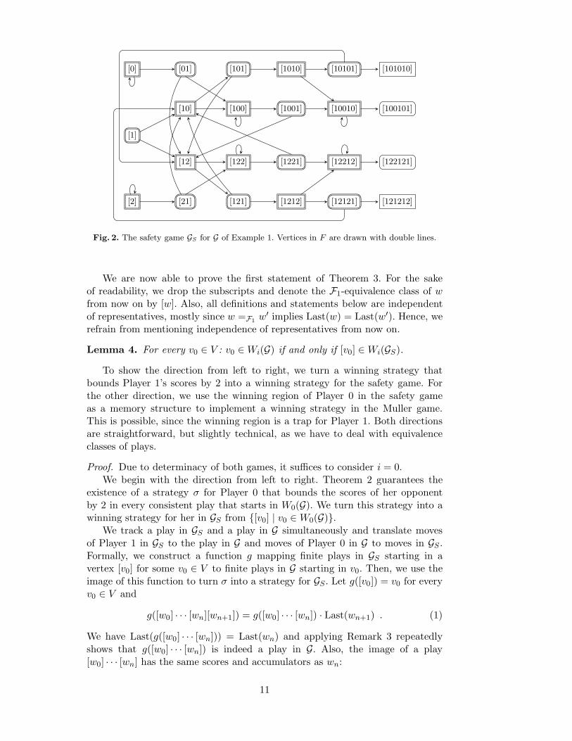
Example 2. The safety game GS for the Muller game G of Example 1 is depictedin Figure 2. One can verify easily that the vertices [v] for v ∈ V are in the winningregion of Player 0.

3 Hence, every vertex in Plays=3

is terminal, contrary to our requirements on an arena. How-ever, every play visiting these vertices is losing for Player 0 no matter how it is continued.To simplify the following proofs, we refrain from defining outgoing edges for these vertices.

10

[1]

[0]

[2]

[01]

[10]

[12]

[21]

[101]

[100]

[122]

[121]

[1010]

[1001]

[1221]

[1212]

[10101]

[10010]

[12212]

[12121]

[101010]

[100101]

[122121]

[121212]

Fig. 2. The safety game GS for G of Example 1. Vertices in F are drawn with double lines.

We are now able to prove the first statement of Theorem 3. For the sakeof readability, we drop the subscripts and denote the F1-equivalence class of wfrom now on by [w]. Also, all definitions and statements below are independentof representatives, mostly since w =F1

w′ implies Last(w) = Last(w′). Hence, werefrain from mentioning independence of representatives from now on.

Lemma 4. For every v0 ∈ V : v0 ∈ Wi(G) if and only if [v0] ∈ Wi(GS).

To show the direction from left to right, we turn a winning strategy thatbounds Player 1’s scores by 2 into a winning strategy for the safety game. Forthe other direction, we use the winning region of Player 0 in the safety gameas a memory structure to implement a winning strategy in the Muller game.This is possible, since the winning region is a trap for Player 1. Both directionsare straightforward, but slightly technical, as we have to deal with equivalenceclasses of plays.

Proof. Due to determinacy of both games, it suffices to consider i = 0.We begin with the direction from left to right. Theorem 2 guarantees the

existence of a strategy σ for Player 0 that bounds the scores of her opponentby 2 in every consistent play that starts in W0(G). We turn this strategy into awinning strategy for her in GS from {[v0] | v0 ∈ W0(G)}.

We track a play in GS and a play in G simultaneously and translate movesof Player 1 in GS to the play in G and moves of Player 0 in G to moves in GS .Formally, we construct a function g mapping finite plays in GS starting in avertex [v0] for some v0 ∈ V to finite plays in G starting in v0. Then, we use theimage of this function to turn σ into a strategy for GS. Let g([v0]) = v0 for everyv0 ∈ V and

g([w0] · · · [wn][wn+1]) = g([w0] · · · [wn]) · Last(wn+1) . (1)

We have Last(g([w0] · · · [wn])) = Last(wn) and applying Remark 3 repeatedlyshows that g([w0] · · · [wn]) is indeed a play in G. Also, the image of a play[w0] · · · [wn] has the same scores and accumulators as wn:

11

Lemma 5. g([w0] · · · [wn]) ∈ [wn].

Proof. By induction over [w0] · · · [wn]. The induction start is immediate due tog([v0]) = v0 ∈ [v0]. So, consider a play [w0] · · · [wn][wn+1]. Since there is an edgefrom [wn] to [wn+1], we have wn ·Last(wn+1) ∈ [wn+1]. By induction hypothesis,we have g([w0] · · · [wn]) =F1

wn and applying Corollary 1, we obtain

g([w0] · · · [wn][wn+1])

=g([w0] · · · [wn]) · Last(wn+1) =F1wn · Last(wn+1) =F1

wn+1 ,

i.e., g([w0] · · · [wn][wn+1]) ∈ [wn+1]. ⊓⊔

Now, we define the strategy σS for Player 0 from {[v0] | v0 ∈ W0(G)} in GS by

σS([w0] · · · [wn]) = [wn · σ(g([w0] · · · [wn]))] ,

i.e., σS translates the play in GS into a play in G and then uses the successor vprescribed by σ to determine the next equivalence class to move to by append-ing v to the current class. We show next that this is always a legal move, providedthe play up to the current position is consistent with σS .

We show inductively that if [w0] · · · [wn] starting in some vertex [v0] for somev0 ∈ V is consistent with σS , then g([w0] · · · [wn]) is consistent with σ andσS([w0] · · · [wn]) describes a legal move in GS. This also implies that σS is awinning strategy from {[v0] | v0 ∈ W0(G)}: assume a play [w0] · · · [wn] starting in[v0] ∈ {[v0] | v0 ∈ W0(G)} consistent with σS leaves F by reaching Plays=3. Thisimplies MaxScF1

(g([w0] · · · [wn])) = 3 since we have g([w0] · · · [wn]) ∈ [wn]. Thus,g([w0] · · · [wn]) starting in v0 ∈ W0(G), being consistent with σ, and reaching ascore of 3 contradicts the fact that σ prevents Player 1 from ever reaching a scoreof 3. Hence, σS is a winning strategy for Player 0 in GS from {[v0] | v0 ∈ W0(G)}.

Since the first statement is clear for the induction start, we only discuss thesecond one in detail: if [v0] ∈ V S

0 , then also v0 ∈ V0 and we have

σS([v0]) = [v0 · σ(g([v0]))] = [v0 · σ(v0)] .

Thus, (v0, σ(v0)) ∈ E and since [v0], [v0 · σ(v0)] ∈ Plays≤2, we conclude also([v0], [v0 · σ(v0)]) ∈ ES , i.e., σS indeed prescribes a legal move.

For the induction step, consider a play [w0] · · · [wn−1][wn] that is consistentwith σS and remember that we have

Last(g([w0] · · · [wn−1])) = Last(wn−1) . (2)

By induction hypothesis, we can assume that g([w0] · · · [wn−1]) is consistentwith σ, hence, it only remains to consider the transition from Last(wn−1) toLast(wn).

If [wn−1] ∈ V S0 , then also Last(g([w0] · · · [wn−1])) ∈ V0 due to (2), and we

have[wn] = σS([w0] · · · [wn−1]) = [wn−1 · σ(g([w0] · · · [wn−1]))] .

Thus, we have Last(wn) = σ(g([w0] · · · [wn−1])). Applying this, the inductionhypothesis, and (1) shows that

g([w0] · · · [wn−1][wn]) = g([w0] · · · [wn−1]) · Last(wn)

12

is indeed consistent with σ.

Now, consider the second statement. By definition, we have

σS([w0] · · · [wn]) = [wn · σ(g([w0] · · · [wn]))] ,

which implies that there is an edge between Last(wn) = Last(g([w0] · · · [wn]))and σ(g([w0] · · · [wn])). Furthermore, g([w0] · · · [wn]) is consistent with σ by in-duction hypothesis, and hence g([w0] · · · [wn]) ·σ(g([w0] · · · [wn])) as well. Since σbounds the scores of Player 1 by 2, both of these finite plays are in Plays≤2

and therefore we can conclude that there is an edge in GS between [wn] and[wn · Last(g([w0] · · · [wn]))], which shows that σS indeed prescribes a legal move.

On the other hand, if [wn−1] ∈ V S1 , then Last(g([w0] · · · [wn−1])) ∈ V1 due

to (2), and we have ([wn−1], [wn]) ∈ ES . Hence, (Last(wn−1),Last(wn)) ∈ E dueto Remark 3. Since Last(g([w0] · · · [wn−1])) = Last(wn−1) ∈ V1 and

g([w0] · · · [wn−1][wn]) = g([w0] · · · [wn−1]) · Last(wn) ,

g([w0] · · · [wn−1][wn]) is indeed consistent with σ.

For the other direction of Lemma 4, we show that W0(GS) can be turnedinto a memory structure for Player 0 in the Muller game that induces a winningstrategy.

Example 3. Consider the winning region W0(G) in the safety game GS of Exam-ple 2 as depicted in Figure 3 (for the sake of readability, we omit two verticesthat are not reachable from a vertex [v] for some v ∈ V ). We obtain a finite-statewinning strategy by using the equivalence class [w] as memory state for a finiteplay w. Since the safety game is the unraveling of the original arena and itswinning region is a trap for Player 1, Player 0 can always prolong a play in theMuller game such that the finite play prefixes w satisfy [w] ∈ W0(GS) no matterwhich successors Player 1 picks. This strategy also bounds the scores of Player 1by two. Hence, it is winning for Player 0.

[1]

[0]

[2]

[01]

[10]

[12]

[21]

[101]

[100]

[122]

[121]

[1001]

[1221]

Fig. 3. The winning region W0(GS) of the safety game GS of Example 2.

13

To simplify the proof, we add one more memory state ⊥, denoting that ascore of 3 was reached. As long as Player 0 sticks to the induced strategy, thismemory state will not be reached. Hence, ⊥ can be eliminated and its incomingtransitions can be redefined arbitrarily.

Define M = (M, Init,Upd,Nxt) by M = W0(GS) ∪ {⊥},

Init(v) =

{

[v] if [v] ∈ W0(G),

⊥ otherwise,

and

Upd([w], v) =

{

[wv] if [wv] ∈ W0(GS),

⊥ otherwise.

Then, for every w ∈ V + with Upd∗(w) 6= ⊥ we have Upd∗(w) = [w]. Further-more, since M is the winning region of a safety game, every [w] ∈ M ∩ V S

0 hasa successor [wv′] for some v′ ∈ V which is in W0(GS) as well. Remark 3 yields(Last(w), v′) ∈ E. Using this, we define the next-move function by

Nxt(v, [w]) =

{

v′ if Last(w) = v and [wv′] as above,

v′′ otherwise, where v′′ is some vertex with (v, v′′) ∈ E,

and Nxt(v,⊥) = v′′ for some v′′ with (v, v′′) ∈ E. The second case in the definitionabove is just to match the formal definition of a next-move function. It will neverbe invoked due to Upd∗(w) = [w] or Upd∗(w) = ⊥.

Let W = {v | [v] ∈ W0(GS)}. It remains to show that σM is a winningstrategy for Player 0 from W . A simple induction shows that every play w thatstarts in W and is consistent with σM satisfies Upd∗(w) 6= ⊥, since the next-move function always prescribes a successor such that the memory is updated toa state in W0(GS). Similarly, Player 1 can only pick successors in G such that thememory is updated to a state in W0(GS), since the winning region of the safetygame (which is the unraveling of the original game modulo =F1

) is a trap forhim. Since we have Upd∗(w) = [w] ∈ Plays≤2 for every play that starts in Wand is consistent with σ, the scores of Player 1 are bounded by 2. Hence, σM isindeed a winning strategy for Player 0 from W . ⊓⊔

The second direction of the proof above also proves the second statement ofTheorem 3.

Corollary 2. Player 0 has a finite-state winning strategy for W0(G) with mem-ory states W0(GS).

To finish the proof of Theorem 3, we determine the size of GS to provethe third statement. To this end, we use the concept of a latest appearancerecord (LAR) [4, 6]. Note that we do not need a hit position for our purposes.

A word ℓ ∈ V + is an LAR if every vertex v ∈ V appears at most once in ℓ.Next, we map each w ∈ V + to a unique LAR, denoted by LAR(w), as follows:LAR(v) = v for every v ∈ V and

LAR(wv) =

{

LAR(w)v if v /∈ Occ(w),

p1p2v if LAR(w) = p1vp2.

14

A simple induction shows that LAR(w) is indeed an LAR, which also ensuresthat the decomposition of w in the second case of the inductive definition isunique. We continue by showing that the LAR of a play w determines all but|Occ(w)| many of w’s scores and accumulators.

Lemma 6. Let w ∈ V + and LAR(w) = vkvk−1 · · · v1.

1. w can be decomposed into xkvkxk−1vk−1 · · · v2x1v1 for some xi ∈ V ∗ withOcc(xi) ⊆ {v1, . . . , vi} for every i.

2. ScF (w) > 0 if and only if F = {v1, . . . , vi} for some i.

3. If ScF (w) = 0, then AccF (w) = {v1, . . . , vi} for the maximal i such that{v1, . . . , vi} ⊆ F .

4. Let ScF (w) > 0 and F = {v1, · · · , vi}. Then, AccF (w) ∈ {∅} ∪ {{v1, . . . , vj} |j < i}.

Proof. 1.) By induction over |w|. If |w| = 1, then the claim follows immediatelyfrom w = LAR(w). Now, let |wv| > 1. If v /∈ Occ(w), then LAR(wv) = LAR(w)vand the claim follows by induction hypothesis.

Now, suppose LAR(w) = p1vp2 with p1 = vk · · · vi+1 and p2 = vi−1 · · · v1,and hence vi = v. By induction hypothesis, there exists a decomposition w =xkvkxk−1vk−1 · · · v2x1v1 for some xi ∈ V ∗ such that Occ(xi) ⊆ {v1, . . . , vi} forevery i. Furthermore, we have LAR(wv) = p1p2v = v′k · · · v

′1 where v′1 = vi,

v′j = vj−1 for every j in the range 1 < j ≤ i, and v′j = vi for every j in the rangei < j ≤ k. Now, define x′1 = ε, x′j = xj−1 for every j in the range 1 < j < i,x′i = xivixi−1, and x′j = xj for every j in the range i < j ≤ k. It is easy to verify,that the decomposition wv = x′kv

′kx

′k−1

v′k−1· · · v′2x

′1v

′1 has the desired properties.

2.) We have ScF (w) > 0 if and only if there exists a suffix x of w withOcc(x) = F . Due to the decomposition characterization, having a suffix x withOcc(x) = F is equivalent to F = {v1, . . . , vi} for some i.

3.) By definition, we have AccF (w) = Occ(x) where x is the longest suffix ofw such that the score of F does not change throughout x and Occ(x) ⊆ F . Con-sider the decomposition characterization of w as above. We have {v1, . . . , vi} ⊆AccF (w), since xivi · · · v1v1 is a suffix of w satisfying Occ(x) ⊆ F . Furthermore,since vi+1 /∈ F by the maximality of i, this is the longest such suffix and we haveindeed AccF (w) = {v1, . . . , vi}.

4.) The lastest increase of ScF (w) occurs after (or at) the last visit of vi,since Occ(vixi−1 · · · x1v1) = F . Hence, AccF (w) is the occurrence set of a suffixof xi−1 · · · x1v1 and the decomposition characterization yields the result. ⊓⊔

The previous characterization allows us to bound the size of GS .

Lemma 7. We have |V S | ≤(∑n

k=1

(

nk

)

· k! · 2k · k!)

+ 1 ≤ (n!)3, where n = |V |.

Proof. We can merge all vertices in V \ F to a single vertex while retaining theequivalence v ∈ Wi(G) ⇔ [v] ∈ Wi(GS) (since f(v) ∈ F for every v ∈ V ) andwithout changing the winning region of Player 0 (since W0(GS) ⊆ F ).

Hence, it remains to bound the number of equivalence classes in Plays≤2 /=F1.

Lemma 6 shows that a finite play w ∈ V + has |LAR(w)| many sets with non-zeroscore. Furthermore, the accumulator of the sets with score zero is determined byLAR(w). Now, consider a play w ∈ Plays≤2 and a set F ∈ F1 with non-zero score.

15

We have ScF (w) ∈ {1, 2} and there are exactly |F | possible values for AccF (w)due to Lemma 6.4, which bounds the number of occurrence sets of suffixes of w.Finally, two finite plays having the same LAR also have the same last vertex.

Hence, the number of equivalence classes is bounded by the number of LARs,which is at most

∑nk=1

(

nk

)

·k!, times the number of possible score and accumulatorcombinations for an LAR of length k, which is at most 2k · k!. ⊓⊔

We conclude this section by mentioning that if one is not interested in computingthe complete winning regions of the Muller game, but only wants to determinewhich player has a winning strategy from a given vertex v, then it suffices toconstruct only the part of GS that is reachable from [v].

Also note that while a player in general can not prevent her opponent fromreaching a score of 2, there are arenas in which she can do so. By first con-structing the safety game G′

S up to threshold 2, which is smaller than the onefor threshold 3, one can possibly determine a subset of Player 0’s winning re-gion faster and obtain a (potentially) smaller finite-state winning strategy forthis subset: we have W0(G

′S) ⊆ W0(GS). However, if Player 0 cannot prevent her

opponent from reaching a score of 2 when starting in v, then this does not implythat Player 1 wins the Muller game from v as well. In this case, one has to solvethe safety game with threshold 3 to determine the winner of the Muller gamefrom this vertex.

4.1 Antichain-based Winning Strategies for Muller Games

Using an antichain construction one can construct a smaller finite-state winningstrategy for Player 0: instead of considering all equivalence classes in the winningregion of Player 0, we only consider the maximal ones with respect to ≤F1

whichare reachable via a fixed positional winning strategy for her in the safety game.To this end, we lift ≤F1

to equivalence classes by defining [w] ≤F1[w′] if and

only if w ≤F1w′.

Let σ be a positional winning strategy for Player 0 in GS and let R be theset of vertices in V S which are reachable from {[v] | [v] ∈ W0(GS)} by playsconsistent with σ. Every [w] ∈ R ∩ V S

0 has exactly one successor in R (which isof the form [wv] for some v ∈ V ) and dually, every successor of [w] ∈ R ∩ V S

1

(which are exactly the classes [wv] for v ∈ V ) is in R.

Now, let Rmax be the ≤F1-maximal elements of R. Applying the facts about

successors of vertices in R stated above, we obtain the following remark.

Remark 4. Let Rmax be defined as above.

1. For every [w] ∈ Rmax ∩ V S0 , there is a v ∈ V with (Last(w), v) ∈ E and there

is a [w′] ∈ Rmax such that [wv] ≤ [w′].

2. For every [w] ∈ Rmax ∩ V S1 and each of its successors [wv], there is a [w′] ∈

Rmax such that [wv] ≤F1[w′].

Thus, instead of updating the memory from [w] to [wv] when processing a ver-tex v, we can directly update it to a maximal element that is F1-larger than [wv].Intuitively, instead of keeping track of the exact scores, we store a maximal ele-ment that over-approximates the exact values.

16

We define M = (M, Init,Upd,Nxt) by M = Rmax ∪ {⊥} 4,

Init(v) =

{

[w] if [v] ∈ W0(GS) and [v] ≤F1[w] ∈ Rmax

⊥ else,

and

Upd([w], v) =

{

[w′] if there is some [w′] ∈ Rmax such that [wv] ≤F1[w′],

⊥ otherwise.

Then, for every w ∈ V + with Upd∗(w) 6= ⊥ we have [w] ≤F1Upd∗(w), which

implies Last(w) = Last(w′), where [w′] = Upd∗(w).Using Remark 4.1, we define the next-move function by

Nxt(v, [w]) =

v′ if Last(w) = v, (v, v′) ∈ E, and

[wv′] ≤F1[w′] for some [w′] ∈ Rmax,

v′′ else, where v′′ is some vertex with (v, v′′) ∈ E,

and Nxt(v,⊥) = v′′ for some v′′ with (v, v′′) ∈ E. Again, the second case in thedefinition above is just to match the formal definition of a next-move function.It will never be invoked due to [w] ≤F1

Upd∗(w) or Upd∗(w) = ⊥.Analogously to the construction in the previous section, it remains to show

that σM is a winning strategy for Player 0 from W = {v | [v] ∈ W0(GS)}. Aninductive application of Remark 4 shows that every play w that starts in W andis consistent with σM satisfies Upd∗(w) 6= ⊥. This bounds the scores of Player 1by 2, as we have [w] ≤F1

Upd∗(w) ∈ Rmax ⊆ Plays≤2 for every such play. Hence,σM is indeed a winning strategy for Player 0 from W .

4.2 Reducing the Number of Memory States

In the proof of Theorem 3 we used the whole winning region W0(GS) of the safetygame as memory structure for a winning strategy of the Muller game. However,when defining the next-move function, we may have to choose between severalvertices v′ with v′ ∈ W0(GS). Depending on this choice, parts of the memorystructure may never be reached (as long as Player 0 sticks to the strategy) and,therefore, can be omitted. Hence, it is possible to reduce the number of memorystates necessary to realize a winning strategy by defining the next-move functionwisely. The same idea applies to antichain-based winning strategies where thefixed strategy σ for the safety game GS determines the size of the set R ofreachable vertices and, hence, of the number of maximal elements.

Unfortunately, it is not clear how to efficiently find a small solution, i.e., aNxt function or strategy σ that induces a small (or even minimal) reachable partof GS . One straightforward heuristic is to compute a “closed” initial part of thesafety game by starting in some initial vertex and considering all successors ofPlayer 1 vertices but only one successor of Player 0 vertices. The choice of thesuccessor in a Player 0 vertex can be made using some order on the successors,or by simply picking an arbitrary one. Another way is to use the automatalearning-based approach described in [8].

4 Again, we use the memory state ⊥ to simplify our proof. It is not reachable via plays thatare consistent with the implemented strategy and can therefore be eliminated.

17

5 Conclusion

We have presented a new algorithm to determine the winning regions of a Mullergame and to determine a winning strategy for one of the players by solvinga safety game. The safety game is polynomially larger than the parity gameobtained in a reduction, but it is faster to solve than the latter.

The scores induce a hierarchy of all finite-state winning strategies, since eachone of them prevents the opponent from reaching a score that is larger than acertain threshold. We suggest to use the highest score the opponent can achieveagainst a given strategy as quality measure for the strategy. In ongoing researchwe investigate whether one can minimize the size of a finite-state strategy andthe scores it allows simultaneously.

Furthermore, it is easy to see that the solution of the safety game actuallyyields a non-deterministic strategy which only disallows those moves that wouldallow the opponent to reach a score of 3 (e.g., see the vertices [1], [01], and [21]in Figure 3). In this sense, our work extends the results of Bernet, Janin, andWalukiewicz [1] on permissive strategies for parity games to Muller games. Inupcoming work, we show that for every fixed k there is a unique most generalnon-deterministic winning strategy that subsumes all strategies preventing theopponent from reaching a score of k.

Acknowledgments We want to thank Wladimir Fridman for many helpfuldiscussions.

References

1. Julien Bernet, David Janin, and Igor Walukiewicz. Permissive strategies: from parity gamesto safety games. ITA, 36(3):261–275, 2002.

2. John Fearnley and Martin Zimmermann. Playing Muller games in a hurry. Int. J. Found.Comput. Sci. To appear. Journal version of [3].

3. John Fearnley and Martin Zimmermann. Playing Muller games in a hurry. In Angelo Mon-tanari, Margherita Napoli, and Mimmo Parente, editors, GANDALF, volume 25 of EPTCS,pages 146–161, 2010. Conference version of [2].

4. Yuri Gurevich and Leo Harrington. Trees, automata, and games. In STOC, pages 60–65.ACM, 1982.

5. Alexander Kechris. Classical Descriptive Set Theory, volume 156 of Graduate Texts in Math-ematics. Springer, 1995.

6. Robert McNaughton. Infinite games played on finite graphs. Ann. Pure Appl. Logic,65(2):149–184, 1993.

7. Robert McNaughton. Playing infinite games in finite time. In Arto Salomaa, Derick Wood,and Sheng Yu, editors, A Half-Century of Automata Theory, pages 73–91. World Scientific,2000.

8. Daniel Neider. Small strategies for safety games. In Proceedings of the Ninth InternationalSymposium on Automated Technology for Verification and Analysis (ATVA 2011), LNCS.Springer, to appear.

18

Aachener Informatik-Berichte

This list contains all technical reports published during the past three years.

A complete list of reports dating back to 1987 is available from

http://aib.informatik.rwth-aachen.de/. To obtain copies consult the above

URL or send your request to: Informatik-Bibliothek, RWTH Aachen, Ahorn-

str. 55, 52056 Aachen, Email: biblio@informatik.rwth-aachen.de

2008-01 ∗ Fachgruppe Informatik: Jahresbericht 2007

2008-02 Henrik Bohnenkamp, Marielle Stoelinga: Quantitative Testing

2008-03 Carsten Fuhs, Jurgen Giesl, Aart Middeldorp, Peter Schneider-Kamp,

Rene Thiemann, Harald Zankl: Maximal Termination

2008-04 Uwe Naumann, Jan Riehme: Sensitivity Analysis in Sisyphe with the

AD-Enabled NAGWare Fortran Compiler

2008-05 Frank G. Radmacher: An Automata Theoretic Approach to the Theory

of Rational Tree Relations

2008-06 Uwe Naumann, Laurent Hascoet, Chris Hill, Paul Hovland, Jan Riehme,

Jean Utke: A Framework for Proving Correctness of Adjoint Message

Passing Programs

2008-07 Alexander Nyßen, Horst Lichter: The MeDUSA Reference Manual, Sec-

ond Edition

2008-08 George B. Mertzios, Stavros D. Nikolopoulos: The λ-cluster Problem on

Parameterized Interval Graphs

2008-09 George B. Mertzios, Walter Unger: An optimal algorithm for the k-fixed-

endpoint path cover on proper interval graphs

2008-10 George B. Mertzios, Walter Unger: Preemptive Scheduling of Equal-

Length Jobs in Polynomial Time

2008-11 George B. Mertzios: Fast Convergence of Routing Games with Splittable

Flows

2008-12 Joost-Pieter Katoen, Daniel Klink, Martin Leucker, Verena Wolf: Ab-

straction for stochastic systems by Erlang’s method of stages

2008-13 Beatriz Alarcon, Fabian Emmes, Carsten Fuhs, Jurgen Giesl, Raul

Gutierrez, Salvador Lucas, Peter Schneider-Kamp, Rene Thiemann: Im-

proving Context-Sensitive Dependency Pairs

2008-14 Bastian Schlich: Model Checking of Software for Microcontrollers

2008-15 Joachim Kneis, Alexander Langer, Peter Rossmanith: A New Algorithm

for Finding Trees with Many Leaves

2008-16 Hendrik vom Lehn, Elias Weingartner and Klaus Wehrle: Comparing

recent network simulators: A performance evaluation study

2008-17 Peter Schneider-Kamp: Static Termination Analysis for Prolog using

Term Rewriting and SAT Solving

2008-18 Falk Salewski: Empirical Evaluations of Safety-Critical Embedded Sys-

tems

2008-19 Dirk Wilking: Empirical Studies for the Application of Agile Methods to

Embedded Systems

2009-02 Taolue Chen, Tingting Han, Joost-Pieter Katoen, Alexandru Mereacre:

Quantitative Model Checking of Continuous-Time Markov Chains

Against Timed Automata Specifications

19

2009-03 Alexander Nyßen: Model-Based Construction of Embedded

Real-Time Software - A Methodology for Small Devices

2009-04 Daniel Klunder: Entwurf eingebetteter Software mit abstrakten Zus-

tandsmaschinen und Business Object Notation

2009-05 George B. Mertzios, Ignasi Sau, Shmuel Zaks: A New Intersection Model

and Improved Algorithms for Tolerance Graphs

2009-06 George B. Mertzios, Ignasi Sau, Shmuel Zaks: The Recognition of Tol-

erance and Bounded Tolerance Graphs is NP-complete

2009-07 Joachim Kneis, Alexander Langer, Peter Rossmanith: Derandomizing

Non-uniform Color-Coding I

2009-08 Joachim Kneis, Alexander Langer: Satellites and Mirrors for Solving In-

dependent Set on Sparse Graphs

2009-09 Michael Nett: Implementation of an Automated Proof for an Algorithm

Solving the Maximum Independent Set Problem

2009-10 Felix Reidl, Fernando Sanchez Villaamil: Automatic Verification of the

Correctness of the Upper Bound of a Maximum Independent Set Algo-

rithm

2009-11 Kyriaki Ioannidou, George B. Mertzios, Stavros D. Nikolopoulos: The

Longest Path Problem is Polynomial on Interval Graphs

2009-12 Martin Neuhaußer, Lijun Zhang: Time-Bounded Reachability in

Continuous-Time Markov Decision Processes

2009-13 Martin Zimmermann: Time-optimal Winning Strategies for Poset Games

2009-14 Ralf Huuck, Gerwin Klein, Bastian Schlich (eds.): Doctoral Symposium

on Systems Software Verification (DS SSV’09)

2009-15 Joost-Pieter Katoen, Daniel Klink, Martin Neuhaußer: Compositional

Abstraction for Stochastic Systems

2009-16 George B. Mertzios, Derek G. Corneil: Vertex Splitting and the Recog-

nition of Trapezoid Graphs

2009-17 Carsten Kern: Learning Communicating and Nondeterministic Au-

tomata

2009-18 Paul Hansch, Michaela Slaats, Wolfgang Thomas: Parametrized Regular

Infinite Games and Higher-Order Pushdown Strategies

2010-02 Daniel Neider, Christof Loding: Learning Visibly One-Counter Au-

tomata in Polynomial Time

2010-03 Holger Krahn: MontiCore: Agile Entwicklung von domanenspezifischen

Sprachen im Software-Engineering

2010-04 Rene Worzberger: Management dynamischer Geschaftsprozesse auf Ba-

sis statischer Prozessmanagementsysteme

2010-05 Daniel Retkowitz: Softwareunterstutzung fur adaptive eHome-Systeme

2010-06 Taolue Chen, Tingting Han, Joost-Pieter Katoen, Alexandru Mereacre:

Computing maximum reachability probabilities in Markovian timed au-

tomata

2010-07 George B. Mertzios: A New Intersection Model for Multitolerance

Graphs, Hierarchy, and Efficient Algorithms

2010-08 Carsten Otto, Marc Brockschmidt, Christian von Essen, Jurgen Giesl:

Automated Termination Analysis of Java Bytecode by Term Rewriting

2010-09 George B. Mertzios, Shmuel Zaks: The Structure of the Intersection of

Tolerance and Cocomparability Graphs

20

2010-10 Peter Schneider-Kamp, Jurgen Giesl, Thomas Stroder, Alexander Sere-

brenik, Rene Thiemann: Automated Termination Analysis for Logic Pro-

grams with Cut

2010-11 Martin Zimmermann: Parametric LTL Games

2010-12 Thomas Stroder, Peter Schneider-Kamp, Jurgen Giesl: Dependency

Triples for Improving Termination Analysis of Logic Programs with Cut

2010-13 Ashraf Armoush: Design Patterns for Safety-Critical Embedded Systems

2010-14 Michael Codish, Carsten Fuhs, Jurgen Giesl, Peter Schneider-Kamp:

Lazy Abstraction for Size-Change Termination

2010-15 Marc Brockschmidt, Carsten Otto, Christian von Essen, Jurgen Giesl:

Termination Graphs for Java Bytecode

2010-16 Christian Berger: Automating Acceptance Tests for Sensor- and

Actuator-based Systems on the Example of Autonomous Vehicles

2010-17 Hans Gronniger: Systemmodell-basierte Definition objektbasierter Mod-

ellierungssprachen mit semantischen Variationspunkten

2010-18 Ibrahim Armac: Personalisierte eHomes: Mobilitat, Privatsphare und

Sicherheit

2010-19 Felix Reidl: Experimental Evaluation of an Independent Set Algorithm

2010-20 Wladimir Fridman, Christof Loding, Martin Zimmermann: Degrees of

Lookahead in Context-free Infinite Games

2011-02 Marc Brockschmidt, Carsten Otto, Jurgen Giesl: Modular Termination

Proofs of Recursive Java Bytecode Programs by Term Rewriting

2011-03 Lars Noschinski, Fabian Emmes, Jurgen Giesl: A Dependency Pair

Framework for Innermost Complexity Analysis of Term Rewrite Systems

2011-04 Christina Jansen, Jonathan Heinen, Joost-Pieter Katoen, Thomas Noll:

A Local Greibach Normal Form for Hyperedge Replacement Grammars

2011-11 Nils Jansen, Erika Abraham, Jens Katelaan, Ralf Wimmer, Joost-Pieter

Katoen, Bernd Becker: Hierarchical Counterexamples for Discrete-Time

Markov Chains

∗ These reports are only available as a printed version.

Please contact biblio@informatik.rwth-aachen.de to obtain copies.

21