Much Ado about Nothing, Almost: Factor Income Distribution in China

Chong-En Bai

Zhenjie Qian

Tsinghua University

Trend since 19784

9.8

13

7.3

41

2.8

5

51

.01

36

.11

12

.87

51

.15

36

.72

12

.13

52

.68

35

.41

11

.9

53

.57

34

.81

11

.63

53

.54

34

.87

11

.59

54

.45

33

.59

11

.96

52

.93

5.0

51

2.0

5

52

.82

34

.67

12

.51

52

.11

35

.39

12

.5

51

.72

35

.22

13

.06

51

.51

35

.21

3.2

9

53

.42

33

.52

13

.06

51

.17

35

.26

13

.57

50

.13

6.5

31

3.3

7

49

.49

36

.46

14

.05

50

.35

35

.83

13

.83

51

.44

35

.61

2.9

6

51

.21

36

.05

12

.74

51

.03

35

.93

13

.04

50

.83

35

.93

13

.24

49

.97

36

.61

3.4

3

48

.71

37

.23

14

.07

48

.23

37

.85

13

.92

47

.75

38

.44

13

.8

46

.16

39

.93

13

.91

41

.55

44

.35

14

.1

41

.44

4.4

81

4.1

2

40

.61

45

.23

14

.16

02

04

06

08

01

00

19

78

19

79

19

80

19

81

19

82

19

83

19

84

19

85

19

86

19

87

19

88

19

89

19

90

19

91

19

92

19

93

19

94

19

95

19

96

19

97

19

98

19

99

20

00

20

01

20

02

20

03

20

04

20

05

20

06

Compensation of employee

Capital income (=operating income + depreciation)

Net taxes on production

Observations

• Capital share increased from 37.34 in 1978 to 45.23 in year 2006.

• Labor share declined from 49.8 in 1978 to 40.61 in 2006.

• Share of taxes on production increased from 12.85 in 1978 to 14.16 in 2006.

• There is an abrupt change between 2003-2004: capital share increased from 39.93 to 44.35, and labor share declined from 46.16 to 41.55.

Trend since 1978 （ net of production taxes)

57.

154

2.8

5

58

.55

41

.45

58.

214

1.7

9

59.

84

0.2

60.

613

9.3

9

60

.56

39

.44

61.

853

8.1

5

60.

153

9.8

5

60.

373

9.6

3

59.

564

0.4

4

59.

494

0.5

1

59.

414

0.5

9

61.

443

8.5

6

59.

214

0.7

9

57.

834

2.1

7

57.

584

2.4

2

58.

424

1.5

8

59.

14

0.9

58.

694

1.3

1

58.

684

1.3

2

58.

584

1.4

2

57.

724

2.2

8

56.

684

3.3

2

56.

034

3.9

7

55

.44

4.6

53.

624

6.3

8

48.

375

1.6

3

48.

215

1.7

9

47

.31

52

.69

02

04

06

08

01

00

19

78

19

79

19

80

19

81

19

82

19

83

19

84

19

85

19

86

19

87

19

88

19

89

19

90

19

91

19

92

19

93

19

94

19

95

19

96

19

97

19

98

19

99

20

00

20

01

20

02

20

03

20

04

20

05

20

06

Compensation of employee

Capital income (=operating income + depreciation)

Questions

• What is behind the recent changes in factor income distribution in China?

• What explains the abrupt changes between 2003 and 2004?

Why Do We Care?

• Factor income distribution may affect size income distribution. – What Is China Doing to Its Workers? (by Arvind S

ubramanian, Peterson Institute, in Business Standard, New Delhi, February 8, 2008):

• This might well be the mother of all redistributions. • Is the dramatic decline in labor's share of the economic

pie ominous?• Will the decline in labor's share of the economic pie be r

eversed through political change? That may be China's big question.

Why Do We Care?

• Factor income distribution may affect size income distribution. – A workers' manifesto for China (Economics focus,

Economist, Oct 11th 2007): “Many countries have seen a fall in the share of labour income in recent years, but nowhere has the drop been as huge as in China. This partly reflects China's large pool of surplus labour, which has depressed wages relative to the economy's large productivity gains.”

Why Do We Care?

• Factor income distribution may affect size income distribution. – Many economists in China have also talked about

the rapid decline in labor share and proposed policies in response to the decline.

– The government has adopted or is considering adopting policies to deal with the issue.

Why Do We Care?• Return to capital

– Investment rate has been increasing. (figure)– Capital output ratio has also been increasing. (figure)– How has the rate of return to capital changed? The answer depends on

capital share. • Kaldor’s stylized facts about the growth of advanced industrial

economy: – Fact one: Real output per capita grows at more or less constant rate ove

r fairly long periods of time– Fact two: The stock of real capital, crudely measured, grows at a more

or less constant rate exceeding the rate of growth of labor input– Fact three: The rates of growth of real output and the stock of capital g

oods tends to be about the same, so that the ratio of capital to output shows no systematic trend

– Fact four: The rate of profit on capital has a horizontal trend– Fact three and four imply that factor income share in output should be

constant

Preview of ResultsSources of the decrease in labor share

Total decrease in labor share from 1995-2004, N1 -10.73 100%

Change in statistical method -6.22 58%

Structural transformation -3.36 31%

Decrease in labor share in industry -1.65 15%

Restructuring of SOEs -0.99

Increase in monopoly power -0.49

Remainder -0.16

Remainder 0.5 -5%

N1: Aggregate Labor share start to decline in 1995

Preview of Results

• The elasticity of substitution between capital and labor in industry sector is not significantly different than 1.

• The change in the relative price of capital and labor is not a significant factor behind the change in labor share in industry sector.

Outline

• What Explains the Abrupt Changes between 2003 and 2004?

• Structural Transformation

• Change of Labor Share in Industry

What Explains the Abrupt Changes between 2003 and 2004?

• Before 2004, all the income of the self-employed was counted as labor income.

• Since 2004, income of the owners of the “individual businesses”, a major form of self-employment other than rural households, has been ascribed as capital income.

• In 2004 census, it’s stipulated that the operating surplus of state-owned and collective-owned farms should be counted as labor compensation and almost half of the provinces follow this method in year 2004, which explains why there is an abrupt increase in the labor share in primary industry.

What Explains the Abrupt Changes between 2003 and 2004?

• Adjustments made using the 2004 census data: – In table 1-26 of China Economic Census Yearbook (NBS, 2007), there

are items such as operating revenue, operating expenditure including employee compensation and payable taxes, book value of fixed assets for individual businesses by industry, which can be employed to calculate value-added, operating surplus for individual businesses by industry according to the method given in DNA (2007).

• Depreciation = book value of fixed assets × 5%• Operating surplus = operating revenue-operating expenditure-depreciation• Net production taxes and labor compensation reported in NBS (2007)• Value added = Depreciation + Operating surplus + Net production taxes +

Employee compensation– We subtract calculated operating surplus of individual businesses from

the reported total operating surplus by industry and add it to employee compensation. With this adjustment, we recalculate labor share.

What Explains the Abrupt Changes between 2003 and 2004?

– We also adjust for the inconsistency between national and provincial data on individual businesses, by assuming that labor productivity of individual businesses at the provincial level is the same as that at the national level.

– As we do not have enough information to judge how much operating surplus of state-owned and collective-owned farms are counted as labor compensation in 2004, we could not make adjustment to eliminate the effect of the associated change. We recalculate aggregate labor share in 2004 using the actual labor share in primary industry in year 2003.

What Explains the Abrupt Changes between 2003 and 2004?

• Adjustments results:

Notes: N1: labor share calculated using reported data; N2: labor share adjusted using Census data; N3: labor share adjusted using Census data and provincial employment numbers in individual businesses; N4: labor share in primary industry in year 2004 is replaced by that in year 2003

• Conclusion– The jump in reported labor share between 2003 and 2004 is

the result of the change in the way we tally the income of the self-employed.

Year Aggregate Primary Industry Construction Tertiary

2003 0.536 0.861 0.444 0.681 0.490

rep_2004,N1 0.484 0.922 0.382 0.598 0.410

ad1_2004,N2 0.643 0.922 0.472 0.659 0.705

ad2_2004,N3 0.555 0.922 0.422 0.625 0.541

ad3_2004,N4 0.546 0.861 0.422 0.625 0.541

Structural Transformation

Year Aggregate Primary Industry Construction Tertiary

1995 0.591 0.883 0.490 0.694 0.486

1996 0.587 0.888 0.486 0.691 0.483

1997 0.587 0.888 0.492 0.694 0.490

1998 0.586 0.889 0.493 0.711 0.492

1999 0.577 0.887 0.488 0.693 0.494

2000 0.567 0.879 0.470 0.706 0.501

2001 0.560 0.876 0.468 0.698 0.498

2002 0.554 0.871 0.462 0.680 0.502

2003 0.536 0.861 0.444 0.681 0.490

2004 0.484 0.922 0.382 0.598 0.410

Labor share by industry

• Observation: – Labor share of the primary sector is much higher than other

industries.– Labor share of the primary sector is overestimated since all

the income of rural households engaged in primary industry production is counted as labor income

Structural Transformation

Year Primary Industry Construction Tertiary

1995 0.230 0.362 0.058 0.350

1996 0.225 0.360 0.057 0.358

1997 0.212 0.362 0.058 0.369

1998 0.201 0.356 0.061 0.381

1999 0.186 0.355 0.062 0.397

2000 0.170 0.362 0.060 0.408

2001 0.162 0.358 0.060 0.421

2002 0.151 0.359 0.060 0.430

2003 0.139 0.375 0.062 0.424

2004 0.142 0.385 0.062 0.410

Structure of the economy

• Observation– The structural transformation resulted in the decline of the primary

sector and rise of the tertiary sector. – As labor share in the primary industry is much higher than that of the

tertiary industry, labor share declined with the structural transformation.

– As labor share in the primary industry is overestimated, the effect of structural transformation would not have been as large if we obtain true estimate of labor share in primary industry

Structural Transformation

• If there’s no structural transformation between 1995 and 2004, then the labor share in 2004 would have been 57%, rather than 53.6%

• Structural transformation can explain 31 percentage points in the change of labor share.

Change in Industry

• Change in labor share in industry explains 15 percentage points in the change in aggregate labor share.

• What has happened?

Change in Industry: Theory

• Utility function

• Production function

• Firm objective: SOEs are interested in the size (output and/or employment) of the firm as well as profits.

• labor share: formula for labor share

• The elasticity of substitution between capital and labor is important.

( ) (1 )( )

i

i i i

i iijt i it ijt i it ijtY a A K a B L

max (1 , 0 1jt jt jt jt jt jtp Y

( )1

(1t jt t jt

Ljtjt jt jt jt

w L A Ka

p Y Y

1

i

i i

iJ

it ijtjU Y

Change in Industry: Predictions

• Ownership effect: labor share is higher when the firm has a stronger size preference.

• Monopoly power: labor share is lower when the firm has stronger monopoly power

• The change in the relative price between capital and labor is reflected in capital-output ratio in efficient term.

• Elasticity of substitution between factors determines the relationship between labor share and capital-output ratio

Change in Industry: Data

• Description of the data– Annual survey of industrial firms conducted by the National Bureau of

Statistics of China from 1998 to 2005. Industrial survey covers all SOEs and non state-owned enterprises with annual sales over 5 million Yuan.

– Capital share: ratio of operating profit and accounting depreciation to value added at factor cost

– Three proxies for monopoly power: price markup; HHI; CR10– Two groups of proxies for ownership: equity shares (req_x); control rig

hts (D_x)– Capital-output ratio: ratio of fixed assets at book value to value added

at factor cost– Capital augmenting technical parameter: controlled by year dummies– Other factors are controlled by industry dummies

Change in Industry: Methodology

• Description of the methodology– System GMM estimation estimates level and difference eq

uations simultaneously, each using lags of difference term and level term of endogenous variables as GMM instruments. This deals with the problem of the endogeneity of capital-output ratio.

– System GMM estimation estimate level equation so that explicit fixed effect such as region dummies and industry dummies can be estimated.

– System GMM estimation uses both between group and within group information when estimating level and difference equation and hence obtain precise estimation for the difference of capital share between enterprises with different ownership structure.

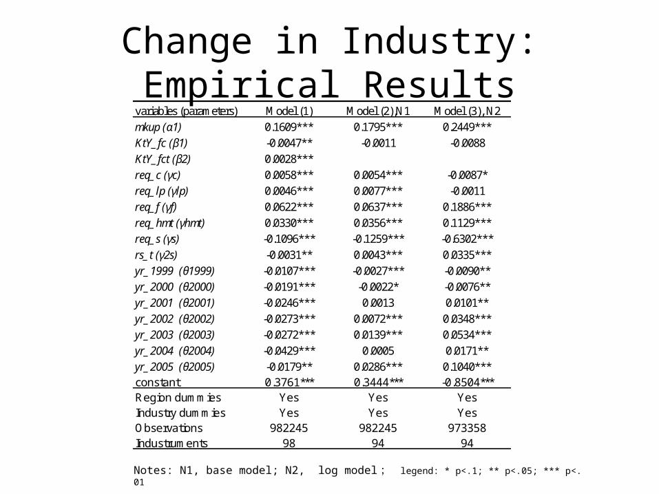
Change in Industry: Empirical Results

Notes: N1, base model; N2, log model ； legend: * p<.1; ** p<.05; *** p<.01

variables (parameters) Model (1) Model (2),N1 Model (3), N2

mkup (α1) 0.1609*** 0.1795*** 0.2449***

KtY_fc (β1) -0.0047** -0.0011 -0.0088

KtY_fct (β2) 0.0028***

req_c (γc) 0.0058*** 0.0054*** -0.0087*

req_lp (γlp) 0.0046*** 0.0077*** -0.0011

req_f (γf) 0.0622*** 0.0637*** 0.1886***

req_hmt (γhmt) 0.0330*** 0.0356*** 0.1129***

req_s (γs) -0.1096*** -0.1259*** -0.6302***

rs_t (γ2s) -0.0031** 0.0043*** 0.0335***

yr_1999 (θ1999) -0.0107*** -0.0027*** -0.0090**

yr_2000 (θ2000) -0.0191*** -0.0022* -0.0076**

yr_2001 (θ2001) -0.0246*** 0.0013 0.0101**

yr_2002 (θ2002) -0.0273*** 0.0072*** 0.0348***

yr_2003 (θ2003) -0.0272*** 0.0139*** 0.0534***

yr_2004 (θ2004) -0.0429*** 0.0005 0.0171**

yr_2005 (θ2005) -0.0179** 0.0286*** 0.1040***constant 0.3761*** 0.3444*** -0.8504***Region dummies Yes Yes YesIndustry dummies Yes Yes YesObservations 982245 982245 973358Industruments 98 94 94

Change in Industry: Robust ChecksBase model Selection of Explained variable

ktsh CR10 HHI D_x

CR10 0.0160***

HHI 0.0465***

mkup 0.1795*** 0.1370*** 0.1675***

KtY -0.0011 0.0006 -0.0012 -0.0012 -0.0039*

req_c 0.0054*** 0.0011 0.0060*** 0.0060***

req_lp 0.0077*** 0.0026** 0.0094*** 0.0094***

req_f 0.0637*** -0.0036 0.0698*** 0.0699***

req_hmt 0.0356*** -0.0303*** 0.0385*** 0.0385***

req_s -0.1259*** -0.1200*** -0.1205*** -0.1205***

rs_t 0.0043*** 0.0039*** 0.0042*** 0.0042***

D_c 0.0075***

D_lp 0.0174***

D_f 0.0687***

D_hmt 0.0323***

D_s -0.1236***

D_s99 0.0018

D_s00 0.0076***

D_s01 0.0130***

D_s02 0.0160***

D_s03 0.0237***

D_s04 0.0334***

D_s05 0.0210***

_cons 0.3444*** 0.3958*** 0.3995*** 0.3489***

variablesSelection of Explanatory Variable

legend: * p<.1; ** p<.05; *** p<.01

Change in Industry: Robust Checks5% sample dropped 10% sample dropped 1998-2003 sample Manufacturing incumbents, N1 incumbents, N2 never restructured

mkup 0.1795*** 0.2788*** 0.2522*** 0.1486*** 0.1688*** 0.1475*** 0.1039*** 0.2365***

KtY -0.0011 0.0001 0.0001 -0.0088** 0.0000433 -0.0034 -0.0071*** -0.0004

req_c 0.0054*** 0.0046*** 0.0042*** 0.0091*** 0.0047*** 0.0044*** 0.0101*** 0.0031***

req_lp 0.0077*** 0.0059*** 0.0059*** 0.0110*** 0.0067*** 0.0060*** 0.0058*** 0.0109***

req_f 0.0637*** 0.0540*** 0.0493*** 0.0844*** 0.0639*** 0.0694*** 0.0862*** 0.0538***

req_hmt 0.0356*** 0.0300*** 0.0273*** 0.0436*** 0.0366*** 0.0374*** 0.0463*** 0.0298***

req_s -0.1259*** -0.1200*** -0.1080*** -0.1001*** -0.1303*** -0.1192*** -0.1006*** -0.1626***

rs_t 0.0043*** 0.0043*** 0.0040*** 0.0041*** 0.0070*** 0.0037*** 0.0020*** 0.0021***

yr_1999 -0.0027*** -0.0024*** -0.0024*** -0.0012 -0.0032*** -0.0035*** -0.0017

yr_2000 -0.0022* -0.0014 -0.0011 -0.0002 -0.0029** -0.0051*** -0.0029** -0.0011

yr_2001 0.0013 0.0036*** 0.0044*** 0.0028** 0.0003 0.0001 -0.0003 0.0008

yr_2002 0.0072*** 0.0100*** 0.0111*** 0.0083*** 0.0065*** 0.0070*** 0.0046*** 0.0075***

yr_2003 0.0139*** 0.0174*** 0.0190*** 0.0145*** 0.0127*** 0.0135*** 0.0099*** 0.0129***

yr_2004 0.0005 0.0055*** 0.0072*** -0.0025 0.0012 -0.0051** -0.0025

yr_2005 0.0286*** 0.0352*** 0.0382*** 0.0261*** 0.0251*** 0.0114*** 0.0255***

_cons 0.3444*** 0.3112*** 0.3207*** 0.3383*** 0.4766*** 0.3497*** 0.3508*** 0.3406***

region dummies Yes Yes Yes Yes Yes Yes Yes Yes

industry dummy Yes Yes Yes Yes Yes Yes Yes Yes

observations 982245 933144 884030 605064 898498 536331 432750 845341

Instruments 94 94 94 83 85 93 94 94

Selection of sampleBase modelvariables

Notes: N1, observations in sample no less than 3 years; N2: observations in sample since 1998; legend: * p<.1; ** p<.05; *** p<.01

Change in Industry: Decomposition

actual

ksh ksh ΔE_mkup ΔE_KtY ΔE_own ΔE_region ΔE_industry ΔE_year

1999-1998 0.0380 0.0176 0.0058 0.0001 0.0116 0.0000 0.0008 -0.0007

2000-1998 0.0752 0.0619 0.0319 0.0004 0.0256 -0.0026 0.0024 0.0042

2001-1998 0.0833 0.0672 0.0255 -0.0013 0.0313 -0.0025 0.0057 0.0085

2002-1998 0.0736 0.0549 0.0161 -0.0010 0.0325 0.0008 0.0020 0.0044

2003-1998 0.0976 0.0646 0.0193 -0.0003 0.0390 0.0013 -0.0008 0.0061

2004-1998 0.0973 0.0588 0.0171 0.0015 0.0402 0.0025 -0.0008 -0.0017

2005-1998 0.1155 0.0935 0.0212 0.0048 0.0467 0.0056 -0.0042 0.0193

PredictedPeriod

－ 81% of actual increase in capital share can be predicted by the model ；－ 1/2 of the predicted capital increase is contributed by ownership restructure－ 1/4 of the predicted capital increase is contributed by monopoly power change－ contribution of the restructure across region and industries is trivial ；

International Comparison• The potential problems with international comparison

– Data compatibility: the tally of income of the self-employed differs across countries– Gollin (2002) estimated labor share by country assuming income of self-employment as c

apital income, comparable to that adopted by the NBS

AUT

BLR

BEL

BOL

BRA

BDI

COG

ECU

FIN FRA

HUN

IND

ITAICT

JAM

JAP

KOR

LVA

MLT

MRT

NLD

NOR

PHLPRTRUN

SWEUKRGBR

USA

VNM

CHN1995

CHN2004

Sources: Gollin (2002) and Author’s calculation

.1.2

.3.4

.5.6

Cap

ital s

hare

acr

oss

coun

trie

s

1/64 1/32 1/16 1/8 1/4 1/2 1

PWTÈ˾ùGDP (U.S.=1)

Rate of Return to Capital: Revised.1

8.2

.22

.24

.26

.28

1980 1985 1990 1995 2000 2005year

unadjustedadjusted

Preview of ResultsSources of the decrease in labor share

Total decrease in labor share from 1995-2004, N1 -10.73 100%

Change in statistical method -6.22 58%

Structural transformation -3.36 31%

Decrease in labor share in industry -1.65 15%

Restructuring of SOEs -0.99

Increase in monopoly power -0.49

Remainder -0.16

Remainder 0.5 -5%

N1: Aggregate Labor share start to decline in 1995

Conclusion

• The elasticity of substitution between capital and labor is not significantly different than 1.

• The change in the relative price of capital and labor is not a significant factor behind the change in labor share.

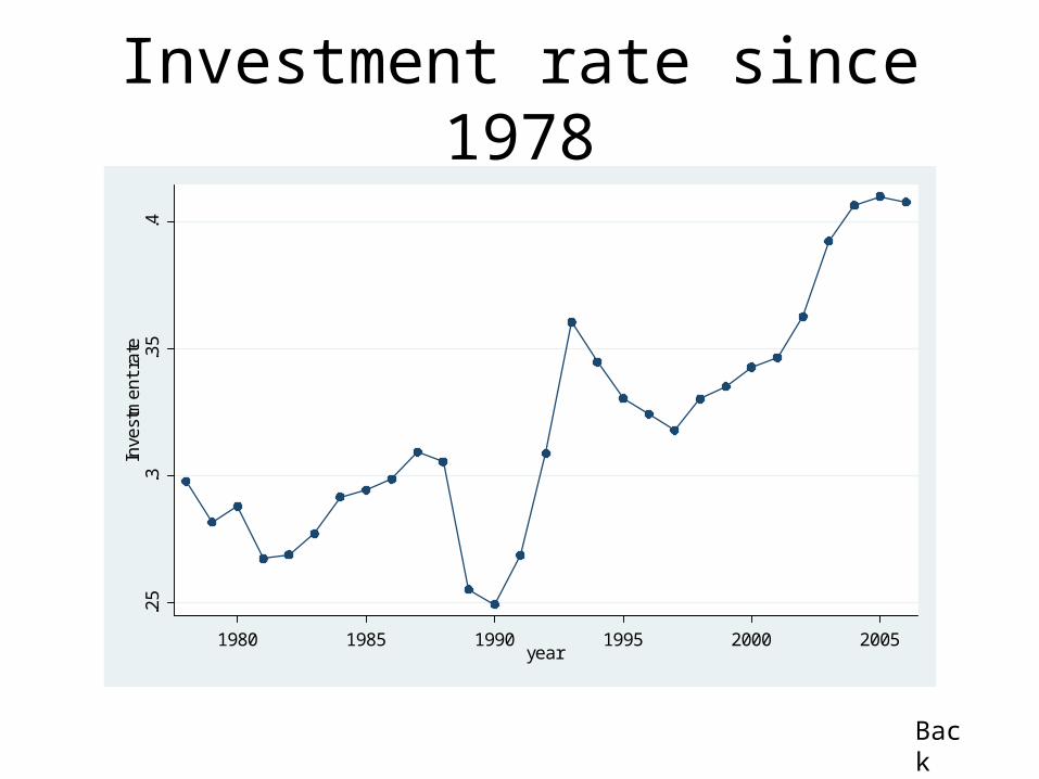
Investment rate since 1978.2

5.3

.35

.4In

vest

men

t rat

e

1980 1985 1990 1995 2000 2005year

Back

Capital-output ratio since 19781.

21.

31.

41.

51.

61.

7C

apita

l-Out

put R

atio

1980 1985 1990 1995 2000 2005year

Back

Structural Transformation

lsh lshc hlsh hlshc hlsh hlshc hlsh hlshc hlsh hlshc

1995 0.591 0.591 0.571 0.571 0.550 0.550 0.490 0.490 0.443 0.443

1996 0.587 0.589 0.567 0.568 0.547 0.548 0.487 0.487 0.448 0.447

1997 0.587 0.594 0.568 0.574 0.549 0.553 0.493 0.492 0.456 0.452

1998 0.586 0.596 0.568 0.576 0.550 0.556 0.496 0.494 0.463 0.456

1999 0.577 0.594 0.561 0.573 0.544 0.553 0.495 0.492 0.461 0.451

2000 0.567 0.589 0.552 0.569 0.537 0.548 0.492 0.488 0.454 0.437

2001 0.560 0.586 0.546 0.566 0.532 0.545 0.490 0.485 0.451 0.431

2002 0.554 0.583 0.541 0.563 0.528 0.543 0.488 0.483 0.448 0.422

2003 0.536 0.570 0.524 0.550 0.512 0.530 0.476 0.471 0.432 0.397

2003-1995 -0.055 -0.021 -0.046 -0.021 -0.038 -0.020 -0.013 -0.019 -0.010 -0.045

yearActual

Hypothetical labor share

10% 20% 50% Chow (1993)

Back