MSU CSE 803

CV: methods of 3D sensing

Structured light;Shape-from-shading;Photometric stereo;Depth-from-focus;

Structure from motion.

MSU CSE 803

Alternate projection models

orthographic weak perspective simpler mathematical models approximations often very good in

center of the FOV can use as a first approximation

and then switch to full perspective

MSU CSE 803

Perspective vs orthographic projection

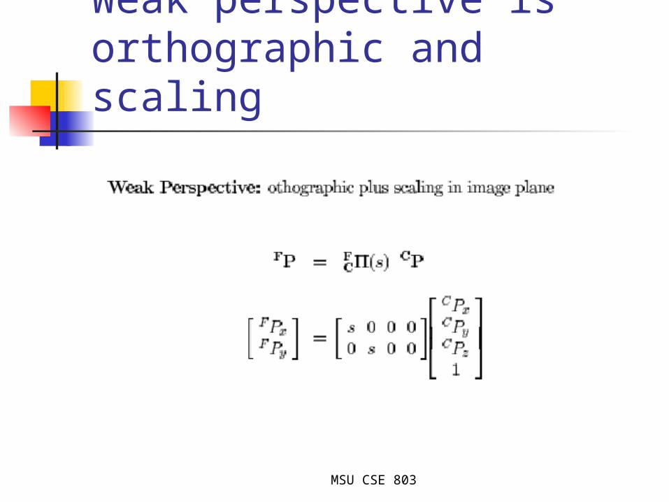
Orthographic is often used in design and blueprints. True (scaled) dimensions can be taken from the image

MSU CSE 803

Orthographic projection

MSU CSE 803

Weak perspective is orthographic and scaling

MSU CSE 803

Study of approximation

MSU CSE 803

P3P problem: solve for pose of object relative to camera using 3 corresponding points (Pi, Qi)

3 points in 3D

3 corresponding 2D image points

MSU CSE 803

What is the “pose” of an object?

“pose” means “position and orientation” work in 3D camera frame defined by a

known camera with known parameters common problem: given the image of a

known model of an object, compute the pose of that object in the camera frame

needed for object recognition by alignment and for robot manipulation

MSU CSE 803

Recognition by alignment Have CAD

model of objects Detect image

features of objects

Compute object pose from 3D-2D point matches

MSU CSE 803

P3P solution approach

MSU CSE 803

General PnP problem “perspective n-point problem” Given: n 3D points from some model Given: n 2D image points known to

correspond to the 3D model points Given: perspective transformation with

known camera parameters (not pose) Solve for the location of all n model

points in terms of camera coordinates, or the relative rotation and translation of the object model

MSU CSE 803

Formal definition of PnP problem

Solutions exist for P3P: in most cases there are 2 solutions; in a rare case there are 4 solutions (see Fischler and Bolles 1981 paper). An interative solution, good for continuous tracking is given below.

A simpler solution using weak perspective has been provided by Huttenlocher and Ullman (1988)

MSU CSE 803

Deriving 3 quadratic equations in 3 unknowns

We know qi; by solving for the 3 ai we will known where each Pi is located

We know the interpoint distances from the model

qi are unit vectors

MSU CSE 803

Iteratively solving 3 equations in 3 unknowns

Want these all to be 0

MSU CSE 803

Approximate via Taylor series

Start with some guessed a1, a2, a3 and move along gradient toward 0,0,0

MSU CSE 803

Solution using Newton’s Method

MSU CSE 803

Our functions have simple partial derivatives

MSU CSE 803

Iteration can be very fast

MSU CSE 803

Notes on this P3P method the equations actually have 8 solutions: 4 are behind the camera (-ai = ai’); 4 are possible, but rare; 2 are common – how to get both solutions? method used by Ohmura et al (1988) to track a

human face at workstation using points outside the eyes and one under the nose

any 3 model points can align with any 3 image points – can match a ship to the image of a face

MSU CSE 803

Using weak perspective algorithm by Huttenlocher and Ullman

is in closed form – no iterations it produces 2 solutions these solutions can be used as

starting points for the iterative perspective method

additional point correspondences can be used to choose correct starting point

MSU CSE 803

Shape from shading methods

Computing surface normals of diffuse objects from the

intensity of surface pixels

MSU CSE 803

Surface normals in C orthographic projection

Radiometry

What determines the brightness of an image pixel?

Light sourceproperties

Surface shape

Surface reflectanceproperties

Optics

Sensor characteristics

Slide by L. Fei-Fei

Exposure

MSU CSE 803

Information used by such algorithms Typically use weak perspective

projection model Brightest surface elt points to light Normal determined to be

perpendicular at object limb Use differential equations to

propagate z from boundary using surface normal.

Smooth using neighbor information.

MSU CSE 803

Results from Tsai-Shah Alg.

Left: from compturer generated image of a vase; right: from a bust of Mozart

MSU CSE 803

Constraint on surface normals

There is a “cone of constraint” for a normal N relative to the light source.

MSU CSE 803

How to use the constraints?

MSU CSE 803

Photometric stereo: calibrate by lighting a sphere, get tables

Estimate the 3D shape from shading information

Can you tell the shape of an object from these photos ?

29

MSU CSE 803

Photometric stereo: 3 lights

MSU CSE 803

Photometric stereo: online

MSU CSE 803

Comments Photometric stereo is a brilliant idea Rajarshi Ray got it to work well even on

specular objects, such as metal parts Requires careful set up and calibration Not a replacement for structured light,

which has better precision and flexibility as evidenced by many applications.

Face Reconstruction in the Wild

MSU CSE 803

Ira Kemelmacher-Shlizerman and Steven M. Seitz. "Face Reconstruction in the Wild." International Conference on Computer Vision (ICCV), Nov 2011.

MSU CSE 803

Depth from focus

Humans and machine vision devices can use focus in a single image to estimate

depth

MSU CSE 803

Use model of thins lens

World point P is “in focus” at image point p ’

MSU CSE 803

Automatic focus technique

Consumer camera autofocus – many methods

One method requires user to frame object in a small window (face?)

Focus is changed automatically until the contrast is the best

Search over focal length until small window has the sharpest features (most energy)

MSU CSE 803

Depth map from focus: concept

for an entire range of focal lengths fi set focal plane at fi and take image for all pixels (x,y) in the image, compute contrast[ fi, x, y]

set Depth[x,y] = max contrast[fi, x, y]

MSU CSE 803

A look at blur vs focal length

Can define resolution limit in line pairs per inch; can define

depth-of-field of sensing

MSU CSE 803

Points P create a blurred image on non optimal image planes

Image plane

Point P is in focus on plane S, but out of focus on planes S’ and S”

MSU CSE 803

How many line pairs can be resolved?

imagine a target that is just a set of parallel black lines on white paper

if lines are far apart relative to the blur radius b, then their image will be a set of lines

if the lines are close relative to blur radius b, then a gray image without clear lines will be observed

MSU CSE 803

Thin lens equation relates object depth to image plane via f

For world point P in focus, then the thin lens equation is:

1/f = 1/u + 1/v

MSU CSE 803

Derivation of thin lens equation from geometry

MSU CSE 803

To compute depth-of-field

the blur changes for different locations via simple geometry

move image forward – get blur move image backward – get blur move image plane to extremes

within limiting blur b and compute depth of field

MSU CSE 803

extreme locations of v set the extremes of u

a is aperture.

By similar triangles

b/a = (v’-v)/v

so

v ’/v = (a+b)/a

MSU CSE 803

Compute near extreme of u

Apply thin lens equation with v’

Note that if b=0, we obtain Un = U

MSU CSE 803

Compute far extreme of u

DEF: The depth of field is the difference between the far and near object planes (Ur – Un) for the given imaging parameters and blur b.

Smaller focal lengths f yield larger DOF.

MSU CSE 803

Example computation

assume f = 50 mm, u = 1000 mm, b = 0.025mm, a = 5 mm Un = 1000 (5 + 0.025) / (5 + 25/50) = 1000 (5.025)/5.5 = 914 Ur = 1000 (5 – 0.025) / (5 – 25/50) = 1000 (4.975)/4.5 = 1106

MSU CSE 803

Example computation

assume f = 25 mm, u = 1000 mm, b = 0.025mm, a = 5 mm Un = 1000 (5 + 0.025) / (5 + 25/25) = 1000 (5.025)/6.0 = 838 Ur = 1000 (5 – 0.025) / (5 – 25/25) = 1000 (4.975)/4.5 = 1244A smaller f gives larger DOF

MSU CSE 803

Large a needed to pinpoint u

changing the aperture to 10 mm Un = 955mm Ur = 1050mm changing the aperture to 20 mm Un = 977mm Ur = 1024mm(See work of Murali Subbarao)

Aperture and DOF

MSU CSE 803

http://www.exposureguide.com/focusing-basics.htm

MSU CSE 803

Structure from Motion

A moving camera/computer computes the 3D structure of the scene and its own motion

MSU CSE 803

Sensing 3D scene structure via a moving camera

We now have two views over time/space compared to stereo which has multiple views at the same time.

MSU CSE 803

Assumptions for now

The scene is rigid. The scene may move or the

camera may move giving a sequence of 2 or more 2D images

Corresponding 2D image points (Pi, Pj) are available across the images

MSU CSE 803

What can be computed

The 3D coordinates of the scene points

The motion of the camera Camera sees many frames of 2D points

Rigid scene with many 3D interest points

From Jabara, Azarbayejani, Pentland

MSU CSE 803

From 2D point correspondences, compute 3D points WP and TR

Factorization method to SfM

[Tomasi & Kanade, IJCV 92]

Structure from Motion 57

Structure [from] Motion Given a set of feature tracks,

estimate the 3D structure and 3D (camera) motion.

Assumption: orthographic projection

Tracks: (ufp,vfp), f: frame, p: point Subtract out mean 2D position… ufp = if

T sp if: rotation, sp: position

vfp = jfT sp

Structure from Motion 58

Measurement equations

Measurement equations ufp = if

T sp if: rotation, sp: position

vfp = jfT sp

Stack them up… W = R S R = (i1,…,iF, j1,…,jF)T

S = (s1,…,sP)

Structure from Motion 59

Factorization

W = R2F3 S3P

SVD W = U Λ V Λ must be rank 3 W’ = (U Λ 1/2)(Λ1/2 V) = U’ V’ Make R orthogonal R = QU’ , S = Q-1V’ if

TQTQif = 1 …

MSU CSE 803

applications

We can compute a 3D model of a landmark from a video

We can create 3D television! We can compute the trajectory of

the sensor relative to the 3D object points

MSU CSE 803

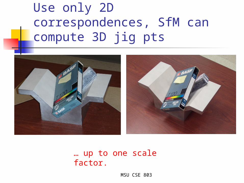
Use only 2D correspondences, SfM can compute 3D jig pts

… up to one scale factor.

MSU CSE 803

http://www1.cs.columbia.edu/~jebara/htmlpapers/SFM/sfm.html

Jabara, Azarbayejani, Pentland

a) Two video frames with corresponding 2D interest points. 3D points can be computed from SfM method.

b) Some edges detected from 2D gradients.

c) Texture mapping from 2D frames onto 3D polyhedral model.

d) 3D model can be viewed arbitrarily!

MSU CSE 803

Virtual museums; 3D TV? Much work, and software, from about 10

years ago. 3D models, including shape and texture

can be made of famous places (Notre Dame, Taj Mahal, Titanic, etc.) and made available to those who cannot travel to see the real landmark.

Theoretically, only quality video is required.

Usually, some handwork is needed.

MSU CSE 803

Shape from Motion methods Typically require careful mathematics EX: from 5 matched points, get 10

equations to estimate 10 unknowns; also a more popular 8 pt linear method

Effects of noise imply many matches needed, still can have large errors

Methods can run in real time Rich literature still evolving http://www.maths.lth.se/matematiklth

/personal/calle/

MSU CSE 803

Special mathematics

Epipolar geometry is modeled Fundamental matrix: computed

from a pair of cameras and point matches

Essential matrix: specialization of fundamental matrix when calibration is available