msc. thesis by - publications listpublicationslist.org/data/ajtp/ref-9/full-paper.pdfthe impact of...
TRANSCRIPT

THE IMPACT OF HUMAN CAPITAL DEVELOPMENT ON
ECONOMIC GROWTH IN ETHIOPIA: EVIDENCE FROM ARDL
APPROACH TO CO-INTEGRATION.
Msc. Thesis
By:
Kidanemariam Gidey Gebrehiwot
June, 2013
Addis Ababa

THE IMPACT OF HUMAN CAPITAL DEVELOPMENT ON
ECONOMIC GROWTH IN ETHIOPIA: EVIDENCE FROM ARDL
APPROACH TO CO-INTEGRATION .
A Thesis Submitted to the Department of Development Economics, Institute of Public
Management and Development Studies (IPMDS), School of Graduate studies,
ETHIOPIAN CIVIL SERVICE UNIVERSITY.
In partial Fulfillment of the Requirements for the Degree of
MASTERS OF SCIENCE IN DEVELOPMENT ECONOMICS
BY
Kidanemariam Gidey Gebrehiwot
June, 2013
Addis Ababa

i
DECLARATION
First, I declare that this thesis is the result of my own work and that all sources or materials
used for this thesis have been duly acknowledged. This thesis has been submitted in partial
fulfillment of the requirements for M.Sc. degree in Development Economics at Ethiopian
Civil Service University and is deposited at the University’s library to be made available to
borrow under the rules of the library. I solemnly declare that this thesis is not submitted to any
other institutions anywhere for the award of any academic degree, diploma, or certificate.
Brief quotations from this thesis are allowable without special permission, provided that
accurate acknowledgement of source is made. Requests for permission for extended quotation
from or reproduction of this manuscript in whole or in part may be granted by the head of the
major department or the Dean of the School of Graduate Studies when in his or her judgment
the proposed use of the material is in the interests of scholarship. In all other instances,
however, permission must be obtained from the author.
Name:__________________
Signature: __________________
Place: ______________________
Date of Submission: June ____, 2013

ii
APPROVAL OF BOARD EXAMINERS
SCHOOL OF GRADUATE STUDIES
ETHIOPIAN CIVIL SERVICE UNIVERSITY
As members of the Examining Board of the Final M. Sc. Thesis Open Defense, we certify that
we have read and evaluated the Thesis prepared by Kidanemariam Gidey Gebrehiwot
entitled The Impact of Human capital Development on Economic Growth and
recommend that the Thesis is accepted as fulfilling the thesis requirement for the degree of
Master of Science in Development Economics.
_________________ _________________ _________________
Name of Chairman Signature Date
________________ _________________ _________________
Name of Major Advisor Signature Date
_________________ _________________ _________________
Name of External Examiner Signature Date
_________________ _________________ _________________
Name of Internal Examiner Signature Date
Final approval and acceptance of the thesis is contingent upon the submission of the final
copy of the thesis to the Council of Graduate Studies (CGS) through the Departmental
Graduate Committee (DGC) of the candidate’s major department.
I hereby certify that I have read this thesis prepared under my direction and recommend that it
be accepted as fulfilling the thesis requirement.
_________________ _________________ _________________
Name of Thesis Advisor Signature Date

iii
BIOGRAPHY
Kidanemariam Gidey Gebrehiwot was born in “Tanbuklo” village near Adigrat city, in Tigray
National Regional State, in the Northern part of Ethiopia on October, 1980. He attended his
elementary and junior education in Abyot-Chora Elementary and junior School at
Shashemene city in Oromiya National Regional State. He attended his high school education
in two schools namely, Shashemene high school and Shire-Endasilasie high school. After
completion of his high school education, he joined Mekelle University and got his B.A.
Degree in Economics in 2006. After that he was employed in Bureau of Finance and
Economic Development (BoFED) of the Tigray National Regional State and served for about
five years as a macroeconomic policy analyst. Then, he joined the Ethiopian Civil Service
University in October, 2011 to follow his postgraduate studies for the M.Sc. in Development
Economics.

iv
ACKNOWLEDGEMENT
This thesis would not have been possible without the support of many people. First and
foremost, I would like to thank to my Advisor, Ato Nahu Asteraye for his valuable guidance,
constructive comments and encouragement which was very important input to conduct this
study. I am also very thankful to my brother Kahsay Tsegay , my brother Kiflemariam Gidey,
my friend Alemaw Berhe and my friend Hintsa Tsigab who has been a source of courage ,
inspiration , and financial & material support in the course of my thesis writing and the whole
learning process. It is with immense gratitude that I acknowledge the reference material
support of Prof. Yilma Gebremariam.
I am also very grateful to my beloved Wife Asmeret Gebreyesus for her practical &
psychological support. As she carried double responsibility in our house and business,
especially in nurturing our lovely daughter (Nardos Kidanemariam), her contribution to the
completion of my paper and the success of my learning process was very fundamental. In
addition, I would also like to acknowledge with much appreciation the crucial role of the
ECSU university leaders & employees; my class mates and other ECSU university students
who surprisingly simplified my mobility problem. A special thank goes to Ato Yemane Yosef
( NBE Vice Governor, Corporate Service), Ato Demirew Getachew (Head, EEA secretariat),
W/rt Eyerusalem (EEA librarian) and my class mates who helped me in data collection.
Furthermore, many thanks go to the head of my department, Ato Gashaw Tsegaye (Head of
the Department of Development Economics), Ato Sherif Muzeyin (Head of the ECSU
Training, Hospitality and Accommodation Support Process), Mahilet Fiseha (Secretary of the
Department of Development Economics), and Baye Sisay (Binding and Sorting Messenger of
the Department of Development Economics) for their responsible administrative support. Last
but not least, I would like to thank to Ato Hailay Tsigab and Ato Tadele Tafese for their
editorial support. Finally, I am also grateful to all who helped me morally and materially on
course of my study.

v
TABLE OF CONTENTS
PAGE
DECLARATION………………………………………..……………....................... i
APPROVAL OF BOARD EXAMINERS…………………………….......................
ii
BIOGRAPHY…………………………………………..………………………….…
iii
ACKNOWLEDGEMENT………………………………………………………...…
iv
LIST OF TABLES………………………………………..……………………….…
viii
LIST OF FIGURES……………………………………………………………..…...
ix
LIST OF APPENDICES……………………………………..……………………....
ix
LIST OF ACRONYMS………………………………………..……………….….…
x-xi
ABSTRACT.................................................................................................................
xii
CHAPTER ONE……………………………………………………………….....…
1
INTRODUCTION……………………………………………….……….…..……..
1
1.1 Background of the Study………………………………………………...….
1-3
1.2 Statement of the Problem……………………………………………...……
3-5
1.3 Research Objectives…………………………………………………..….… 5
1.4 Research Questions…………………………………………………...……. 5
1.5 Significance of the Study………………………………………………..…. 5
1.6 Scope and Limitation of the Study…………………………………………
6
1.7 Organization of the Study………………………………………………..…
6
CHAPTER TWO…….……………………………………………………………..
7
LITERATURE REVIEW………………………………………………………..…
7

vi
TABLE OF CONTENTS(Continued)
2.1 Theoretical Literature Review…………………………………………….… 7
2.1.1 Human capital and neoclassical growth theories………………...…
7-8
2.1.2 Human capital and endogenous growth theories……………….….
8-9
2.1.3 Investment in education and returns to education …………..…….
9-11
2.1.4 Health and human capital……………..…………………………...
11
2.1.5 Rationale for public intervention in education and health………....
12
2.1.6 Measuring human capital ……………………..……………….......
12-14
2.2 Empirical Literature Review…………………………………………….…
15-17
CHAPTER THREE………………………………………………….………..……
18
OVERVIEW OF ECONOMIC GROWTH, EDUCATION AND HEALTH
SECTORS IN ETHIOPIA……………………….………………..………..………
18
3.1 Public Spending on Education and/or Health in Ethiopia…………….…....
18-20
3.2 Life Expectancy and Death rate………………………………………..…...
20
3.3 Enrolment rate and Educational Attainment…………………………….....
21-22
3.4 Trends of Real GDP and Per Capita Income Growth in Ethiopia……….....
23-24
CHAPTER FOUR……………………………………..……………………….…...
25
MODEL SPECIFICATION AND METHODOLOGY…………………….….....
25
4.1 Theoretical Framework and Model Specification………………….…...….
25-29
4.2 Data Sources and Measurement of Variables………………………........…
29-33
4.3 Methodology of the study……………………………………….…….…....
34
4.3.1 Stationarity and non-stationarity of time series data………………
34

vii
TABLE OF CONTENTS (Continued)
4.3.2 Unit root testing……………………….…………………….…….. 34-37
4.3.3 Co-integration Analysis and Vector Error Correction Model……..
37-44
CHAPTER FIVE……………………………………………………………..…......
45
RESULTS AND DISCUSSION……………………………………...………...…..
45
5.1 Augmented Dicky-Fuller Unit Root Test…………………………...…..….
45-46
5.2 Long run ARDL Bounds Tests for Co- integration…………………….…...
46-47
5.3 Long-Run Model Estimation………………………………………….....…
47-49
5.3.1 Long-run diagnostic tests………………………………...………..
49-51
5.4 Short Run Error Correction Estimates………………………………...…....
51-53
5.4.1 Short-run diagnostic tests…………………………...……………..
53
5.5 The Pairwise Granger Causality Results………………………….…….......
53-54
CHAPTER SIX…………………………………………………………….………..
55
CONCLUDING REMARKS AND POLICY IMPLICATION……………..…...
55
6.1 Conclusion…………...……………………………………………………...
55-56
6.2 Policy Implication…………………………………………………………...
56-57
REFERENCE
Annex

viii
LIST OF TABLES
PAGE
Table 1. Percentage of economically active population (age 15-64) by educational
attainment……………………………………………………...….........…
22
Table 2. Summary of data source by variable…………………………………..…..
30
Table 3. ADF unit root test results……………………………………...…….….…
45
Table 4. Pesaran et al.(2001) and Narayan (2005) critical value…………...…....…
46
Table 5. Bounds test for co- integration Analysis………………….…........……......
47
Table 6. Estimated long run coefficients using the Autoregressive Distributed Lag
Approach : ARDL(1,0,2,2,2,2,1) selected based on Akaike Information
Criterion………………………………………………………………...…
47
Table 7. Long-run diagnostic tests………………………………….……................
49
Table 8. Error correction representation for the selected Autoregressive
Distributed Lag Model: ARDL (1,0,2,2,2,2,1) selected based on
Akaike Information Criterion……...............................................................
52
Table 9. Short-run diagnostic tests…………………………….………..…..............
53
Table 10. Granger causality test………………...……………………..………….....
54

ix
LIST OF FIGURES
LIST OF TABLES IN THE APPENDIX
Table-A. Autoregressive Distributed Lag estimates (Dynamic estimation results):
ARDL(1,0,2, 2,2,2,1) selected based on Akaike information Criterion
Table-B. Estimated model for Wald test (Bound test)
PAGE
Figure 1. Trends in the share of public spending on education and/or Health
to GDP and total government expenditure in Ethiopia….........................…
19
Figure 2. Trends of life expectancy and death rate…………………………….....…
20
Figure 3. Trends of gross enrolment rate in Ethiopia………………………….........
21
Figure 4. Trends of real GDP and per capita income growth in Ethiopia…….....…
23
Figure 5. Plot of cumulative sum of recursive residuals…………………...…....…
50
Figure 6. Plot of cumulative sum of squares of recursive residuals……...….......…
50

x
LIST OF ACRONYMS
AIC……………………
Akaike Information Criterion
AR (1)………………… Autoregressive Order One
ARDL………………… Autoregressive Distributed Lag
ADF………………...… Augmented Dicky Fuller
CGE…………………... Computable General Equilibrium
CSLS………………….. Centre for the Study of Living Standards
CUSUM………………. Cumulative Sum of Recursive Residuals
CUSUMSQ…………… Cumulative Sum of Squares of Recursive Residuals
DF………………...…... Dicky Fuller
DW……………………. Durbin Watson
ECT…………………... Error Correction Term
EEA/EEPRI………….. Ethiopian Economic Association/Ethiopian Economic Policy
Research Institute
EEA/EEPRI………….. Ethiopian Economic association
FDRE……………….… Federal Democratic Republic of Ethiopia
GDP………………...… Gross Domestic Product
HSDP……………….… Health Sector Development Plans
ILO…………………… International Labor Organization
MOE………………….. Ministry of Education
MOH………………….. Ministry of Health
MOFED………………. Ministry of Finance and Economic Development
NBE………………...… National Bank of Ethiopia
NGO………………...… Non-Governmental Organizations
ODA…………………... Official Development Assistance

xi
LIST OF ACRONYMS (Continued)
OECD………………… Organization for Economic Co-operation and Development
OLS…………………… Ordinary Least Square
UNCTAD…………...… United Nations Conference on Trade and Development
UNESCO……………... United Nations Educational, Scientific and Cultural Organization
USD…………………… United States Dollar
UNDP…………………. United Nations Development Programme
VECM………………... Vector Error Correction Model
WB……………………. World Bank
WDE………………….. World Data on Education

xii
ABSTRACT
The main objective of the study was to investigate the long run and short run impact of human capital
on economic growth in Ethiopia (using real GDP per capita, as a proxy for economic growth) over the
period 1974/75-2010/2011. The ARDL Approach to Co-integration and Error Correction Model are
applied in order to investigate the long-run and short run impact of Human capital on Economic
growth. The finding of the Bounds test shows that there is a stable long run relationship between real
GDP per capita, education human capital, health human capital, labor force, gross capital formation,
government expenditure and official development assistance. The estimated long run model revels that
human capital in the form of health (proxied by the ratio of public expenditure on health to real GDP)
is the main contributor to real GDP per capita rise followed by education human capital (proxied by
secondary school enrolment). Such findings are consistent with the endogenous growth theories which
argue that an improvement in human capital (skilled and healthy workers) improves productivity. In
the short run, the coefficient of error correction term is -0.7366 suggesting about 73.66 percent
annual adjustment towards long run equilibrium. This is another proof for the existence of a stable
long run relationship among the variables. The estimated coefficients of the short-run model indicate
that education is the main contributor to real GDP per capita change followed by gross capital
formation (one period lagged value) and government expenditure (one period lagged value). But,
unlike its long run significant impact, health has no significant short run impact on the economy. Even
its one period lag has a significant negative impact on the economy.
The above results have an important policy implication. The findings of this paper imply that
economic performance can be improved significantly when the ratio of public expenditure on health
services to GDP increases and when secondary school enrolment improves. Such improvements have
a large impact on human productivity which leads to improved national output per capita. Hence
policy makers and / or the government should strive to create institutional capacity that increase
school enrolment and improved basic health service by strengthening the infrastructure of educational
and health institutions that produce quality manpower. In addition to its effort, the government should
continue its leadership role in creating enabling environment that encourage better investment in
human capital (education and health) by the private sector.
Key words : Ethiopia, Economic Growth, Human capital, Education, Health, ARDL method of Co-
integration, ECM model.

1
CHAPTER ONE
INTRODUCTION
1.1 Background of the Study
With its large reserves of human and natural resources, Ethiopia should have been a
prosperous economy with low poverty level, improved infrastructure services, better
education and health status. However, it is one of the poorest countries in the world
manifested by low per capita income and low human development index. According to Word
Bank (2011) data, the real per capita income level of the country was 141.86 USD in
1981.This figure has decreased with some fluctuations for the next 11 years and reached to
115.8 USD in 1991. After the overthrow of the military regime, real per capita income level
showed a continuous improvement for the next 5 years and reached to 125.58 USD in
1996/97. But, in the next 6 years generally declined (with some ups and downs) to 124.30
USD in 2003 .Starting from 2004, it has increased continuously and reached to 231 USD in
2011. On the other hand, in 2000, human development index of the country was 0.274. This
figure has slightly increased to 0.363 in 2011 (UNDP, 2011).
Modern theory of economic growth argues that human capital, especially education and health
has the principal role on achieving economic growth and development (Gyimah-Brempong
and Wilson, 2005). In line with this, Ethiopia has made some movements to create skilled and
competent citizens through designing different education and health policies and
implementing them.
Before 1925, in Ethiopia, education was limited to religious institutions. After that,
recognizing the importance of education, the imperial regime has tried to design a plan that
expands secular education in the country (Oumer, 2007). During the military regime,
educational program was formulated with the slogan of education for production, education
for scientific realization, and education for political consciousness (Woubet, 2006). But,
limited provision, inequitable distribution, inefficiency, irrelevance and poor quality were
fundamental problems of education prior to 1991(MOE, 2008). In 1974/75 the ratio of
expenditure on education to total GDP was 1.58 percent and declined for the next seven years.

2
After 1981/82, it has showed a slight increment and reached to 1.92 in 1989/90
(EEA/EEPRI, 2010 and MoE ,2011).
In addition to the education sector, at the beginning of the military regime, a new health
policy which emphasizes on disease prevention and control and rural health services was
designed. Further, the government formulated a ten-year health perspective plan as part of the
ten-year economic development plan launched in 1984. The goal of this plan was providing
basic health services to the majority of the population (Mongabay, 2010).To achieve this goal,
health stations, health centers, rural hospitals, regional hospitals, and central referral hospitals
were supposed to provide proper health care to the society. However, by the late 1980s, these
facilities were available to only a small fraction of the country's population (Ibid).
After the overthrow of the military regime, in 1994 education Sector Strategy was designed
by the current government (WDE, 2010). The main focuses of the strategy was: changing
curriculum; expanding primary, secondary and tertiary level education; improving the quality
of education ; making education more relevant to the demands of the community;
restructuring the organization and administration of the education system (Ibid). According to
EEA/EEPRI, (2010) and MoE (2011) data, the ratio of educational expenditure to total GDP
was around 1.64% in 1991/92 .This has generally increased for the next twenty years and
reached to 4.57 % in 2010/11.
As one part of its socioeconomic measures, FDRE government has also developed national
health policy and comprehensive Health Sector Development Plans (HSDPs) in 1996/97.
Democratization and decentralization of the health care system; developing preventive and
curative components of health care; creating accessible health care service for all parts of the
population; and encouraging private and NGO participation in the health sector were the main
goals of the policy). During the past fifteen years, the government has made an inspiring
skeleton for improving the health of the people (MOH, 2010). Expenditure on health as a
percentage of GDP was 3.89% in 1995 and after ten years it reached to 4.89% with some
slight fluctuations in the middle (UNESCO ,2010) .But, the desired outcome is not achieved
yet, though some major efforts are done (MOH , 2010).

3
As we have seen above, though the degree of emphasis and success may vary from one
regime to another, an effort has been made to increase the productivity of the citizens and the
total income of the country.
1.2 Statement of the Problem.
Human capital refers to the “knowledge, skills, competence and attributes embodied in
individuals that facilitate the creation of personal, social and economic well-being” (OECD,
2001:17). Recent growth literature has given more emphasis to the consequence of human
capital in economic growth and development .Generally; economic growth and development
theorists argued that human capital has a substantial effect on economic growth and
development (Kefela and Ren, 2007). For instance, According to Harbison (1971) wealth of a
nation is critically determined by its level of human capital. For him , differences in the level
of socio-economic development across nations is determined not so much by natural
resources and the stock of physical capital but by the quality and quantity of human resources.
Similarly, Lucas (1988); Romer (1990); Mankiw, Romer, and Weil (1992 and Bergheim
(2005) argued that human capital is crucial so as to increase the productivity of labor and
physical capital. In addition, ILO report (2003) as cited by Patron (2006: 3) states that, “the
knowledge and skills endowment of a country’s labor force, rather than its physical capital,
determines its economic and social progress, and its ability to compete in the world
economy”. In other words, human capital is the main source of knowledge and a guide for the
implementation of this knowledge in the production process.
Even though there is an argument on the importance of human capital for economic growth of
any country, it is still controversial that what factors should be considered as human capital
and how to measure it. In most of the studies education or health related indicators are
employed as a proxy for human capital (Qadri and Waheed, 2011).
Like other countries, Ethiopia has devoted much resource and efforts to the ed ucation and
health sectors anticipating productivity improvement of the citizens and thereby economic
growth. These resources are cost to the society not only because they are economic resources
but also because they have alternative uses. Therefore, inves tigating the relationship between

4
human capital (resources devoted to this sector) and economic growth may be a big concern
to policy makers and even to the society.
Some researchers have tried to investigate the relationship between human capital
development and economic growth in Ethiopia. For instance, using school enrollment as a
proxy for human capital, Seid (2000) found an insignificant impact of human capital on
output level. Similarly Wubet (2006) has got the same result that proves the non existence of
any relationship between the two macroeconomic variables. But, their approach of measuring
human capital ignores the health aspect of human capital development, while both education
and health are important component of human capital.
On the other hand, using public spending on education and health sector as a proxy for
investment in human capital development, Teshome (2006) found a positive impact of
human capital development on economic growth in Ethiopia. This finding is reinforced by
Tofik (2012) who found a positive and significant relationship between capital spending on
human capital and economic growth. But both of them didn’t show the separate impact of the
health and education sector on economic growth. In addition Tofik failed to incorporate the
recurrent human capital expenditure account of the government. Since both education and
health are important elements of human capital, using both indicators is relatively better
measure of human capital than using education or health indicators a lone. Therefore, the
author of this paper has used both the education and health indicators so as to empirically
analyze the effects of human capital development on economic growth by taking secondary
school enrolment rate as a proxy for human capital in the education area and the ratio of
public expenditure on health to GDP as a proxy for human capital in the health area.
All of the above researchers who tried to identify the relationship between human capital and
economic growth in Ethiopia have used the same technique of analysis (Johnson’s Co-
integration technique). Even though the Johnson’s Co-integration technique is one of the
widely used methods of time series analysis, its outcome could not be reliable for small
sample size (Pesaran and Shin, 1997; Narayan, 2005; Udoh and Ogbuag, 2012). Relatively,
the Autoregressive distributed lag method of co- integration has more advantage over the
Johnsons method (Pesaran and Shin, 1997; Pesaran and Shin, 1999; Pesaran, Shin, and Smith,

5
2001; Harris and Sollis, 2003; Narayan, 2005; Chaudhry & Chaudhry, 2006; Ang ,2007 and
Rahimi and Shahabadi , 2011). Hence this paper has used this approach to provide valid
empirical evidence on the effects of human capital development on economic growth.
1.3 Research Objectives
The main objective of the study is to analyze the impact of human capital development on
economic growth in Ethiopia over the period 1974/75-2010/11. The study will try to address
the following specific objectives:
To empirically evaluate the impact of human capital development on economic
growth in Ethiopia, both in the short-run and in the long-run.
To analyzes the causal relationship between human capital development and
economic growth in Ethiopia.
To derive policy implications from the empirical analysis.
1.4 Research Questions
Does human capital development have a significant long-run and short-run impact
on economic growth in Ethiopia?
Is there a causal relationship between human capital development and economic
growth in Ethiopia?
1.5 Significance of the Study
This study is expected to generate the following benefits:
It will improve the practical knowledge and skill of the researcher of this study by
making familiar with factual evidence on the macroeconomic problems.
It will produce general information on the relationship between human capital
development and economic growth.
It will serve as a spring board for further studies on human capital development and
economic growth.
It will generate evidences for policy implications that aim to analyze the interaction of
human capital development and economic growth.

6
1.6 Scope and Limitation of the Study
The study has used 37 years annual data covering from the period 1974/75 to 2010/11.The
study excludes comparative analysis with other countries. In order to empirically analyze the
long run and short run relationship between human capital development and economic growth
(real GDP per capita), only secondary school enrolment is used as a proxy for the education
human capital. On the other hand, the ratio of total government expenditure on health to GDP
is used as a proxy for health human capital indicator. In this research, though learning on the
job (experience) could have an impact on human capital development, only formal education
is used as a proxy for human capital formation in the education area. On the other hand, the
research didn’t include the impact of private expenditures on health. But, s ince most of the
basic health service is provided by the government, government expenditure on health can
explain the health human capital created in Ethiopia. Further, though only two variables (labor
force and official development assistance) are taken from international organizations
(UNCTAD and WB), such mixed sources of data may have little impact on the quality of the
results.
1.7 Organization of the Study
The paper has six chapters .The first chapter deals with the introduction part of the paper.
Chapter two reviews the theoretical and empirical literature regarding human capital and
economic growth. The third chapter presents the overview of economic growth, education and
health sectors in Ethiopia. Chapter four addresses the model specification and methodology
aspect of the paper. The fifth chapter concentrates on the results and discussion part of the
paper. And finally, the conclusion and recommendation part is presented in the sixth chapter.

7
CHAPTER TWO
LITERATURE REVIEW
2.1 Theoretical Literature Review
Before the modern human capital theories come to literature, a given economy is mostly
believed to depend only on physical capital (land, machinery and equipment) and raw Labor.
Investment in capital equipment was largely assumed the dominant factor of output. For
instance, the classical theorists give much focuses on the exploitation of labor by capital
(Marimuthu, Arokiasamy and Ismail, 2009).However, after 1950s some modern economists
come and formally treat education and health as the key factors in improving human capital
and thereby increasing economic progress ( Kern, 2009 ).
2.1.1 Human capital and neoclassical growth theories
Schultz (1961) and Becker (1962) are among the first human capital theorists. According to
them, education augments individual’s skill and thus his or her human capital. A higher skill
level in the workforce increases the production capacity. On the other hand, Schultz (1975) as
cited by Xiao (2001) suggests that education enables individual workers to adjust themselves
in accordance with changing economic conditions by understanding any shocks, analyzing
information, and reallocating resources. On the other hand, Spence (1973) perceived
education as a market signal for the potential productivity of workers. It also serves as a
screening tool to select potential workers that can be trained for specific jobs more quickly
and at a lower cost than their counterparts. But their argument was not practically
incorporated in to economic growth theories until the standard neoclassical growth model was
revised by Mankiw, Romer, and Weil in the year 1992. These scholars have used a Cobb-
Douglas production function to reexamine the Solow growth model.
Generally, neoclassical growth theory argues that long-term economic growth is determined
solely by the accumulation of factor inputs such as physical capital and labor. Studies reveal a
significant contribution from technical progress, which is defined as an exogenous factor.
Solow (1957) and Cass (1965) are among those who first demonstrated this. They propose the

8
convergence theory of growth which treats technology as the sole long run determinant of
growth.
Generally, they said that, in the long run, sustained positive growth rate of output per capita is
only apparent if there is continues advances in technological knowledge in the form of new
goods, new markets, or new processes. If there is no technological progress, then the effects
of diminishing returns would eventually cause economic growth to cease. When we continue
to provide people with more and more of the same capital goods without inventing new uses
for the capital, then the extra capital goods become redundant and therefore the marginal
product of capital will become negligible. This idea is captured formally by assuming the
marginal product of capital to be strictly decreasing in the stock of capital (Aghion and
Howitt, 1998). In other words, assuming diminishing returns to scale, they said that as capital
per worker increases, growth of the economy slows down until it reaches the steady state and
the lower the initial level of income per capita the higher is the predicted growth rate (Weil,
2009). But the model cannot explain the existence of continuous economic progress like the
case of East Asian developing economies (Zarra-Nazhad & Hosainpour, 2011).
2.1.2. Human capital and endogenous growth theories
In order to address the limitations of the neoclassical theory and answer the long-run
determinants of economic growth, in the mid 1980s, endogenous growth models were
developed. Lucas (1988) and Romer (1990), who are the famous proponents of this theory,
include deliberately created technological changes as an explanatory variable in their growth
model. For endogenous growth theorists, it is not only technology which determines the
growth of a given nation, but there are other factors (such as human capital) that are not
captured by the neoclassical growth model.
Lucas (1988) considers human capital as a separate input in the production function formed
predominantly by workers through education or on-the-job training. In the Lucas (1988)
model, the rate at which human capital is being accumulated was seen as the cr itical
determinant of productivity growth.

9
On the other hand Romer (1990) treats human capital as a factor affecting innovation that
have a positive impact on the long-run rate of productivity growth, instead of treating human
capital as a direct input to the production of goods. That means, for Romer endogenous
growth is caused by accumulating technology /knowledge while for Lucas it is the non-
decreasing marginal returns of human capital that creates endogenous growth.
Generally, they conclude that just having a large population is not sufficient to generate
growth, rather stock of human capital and research and development are sources of economic
growth. According to these models, the law of diminishing returns to scale may not be true
since the returns on physical and human capital goods do not necessarily diminish through
time. If the owner of the capital employs a skilled and healthy worker, the productivity of the
capital and the technology will improve. Another justification to the possibility of increasing
returns to scale is the spillover of knowledge across producers and external benefits from
improvements in human capital (Wilson and Briscoe, 2004).
Similarly, in order to re-examines the Solow growth model and to explain the cross country
per capita income variation, Mankiw, Romer, and Weil (1992) has formulated an augmented
Solow model, in which human capital enters as a factor of production with those of physical
capital and raw labor. They conclude that differences in human capital, saving and population
growth determines cross-country differences in income per capita. That means accumulation
of physical capital and population growth has greater impacts on income per capita when
human capital is taken into account in the model. According to the above researchers,
excluding it from the model may result in biased results.
2.1.3. Investment in education and rate of returns to education
The time and money spent in formal schooling, on-the job-training and off-the-job training
are the main investments in education. These investments involve direct tuition expenditures,
foregone earnings during schooling, and reduced wages during training that are incurred in
order to gain a return on this investment in the future. Becker (1993) in his book entitled
“Human Capital: A Theoretical and Empirical Analysis with special reference to education”
argues that there are different kinds of investments in human capital that include schooling,
expenditures on medical care, on job training and others. In other words, investment in human

10
capital refers to activities that influence future real income through the embedding of
resources in people. So, to him investment on education and training is the most important
issue to create human capital. Giving more emphasis to education, he justified that education
and training raise the productivity of workers by providing useful knowledge and skills.
Generally, the costs of education and the employment opportunities after education are the
two key determinants of the private returns to education (Rephann, 2002, cited in
Fleischhauer, 2007). As with investments in physical capital, a human capital investment is
only undertaken if the expected return from the investment (which is equal to the net internal
rate of return) is greater than the market rate of interest. That means, schooling is an
investment that is undertaken expecting future income for individuals who receive it.The
return to education comes through the channel of increased earnings for the worker and higher
productivity for the firm as well as increased employment probabilities (Ibid).
According to Mincer (1981, 1989, 1996) wages /return of a worker are determined by the size
of his/her human capital stock. As a result wage disparity among workers is mainly due to the
variation in the sizes of human capital stocks not due to the raw labor. The returns to
education are not solely private. There may be spillovers from education to other individuals,
in which case the social benefits would be higher than the sum of private returns to educated
individuals. McMahon (1998, 2010) has classified the returns to education as monetary and
non-monetary as well as private and social. Wages are the direct private and monetary returns
from education. The effects of education on GDP growth and on the earnings of others (by
making them more productive) are also other forms of monetary social benefits /returns.
Beyond the monetary benefits, education may have non monetary benefits to individuals as
well as to the society as a whole. (Ibid, 2010). Health effects, more efficient household
management, lifelong adaptation and continued learning at home (use of new technologies as
Internet, radio and television, educational reading etc.), non monetary job satisfaction, are
some of the non-monetary private returns. The gains from living in an educated society (better
citizenship, democracy stability, poverty reduction and lower crime rates) and community
services from education (dissemination of knowledge through articles, books, media and also
informally) are some of the examples of on-monetary social benefits. In addition, it may
facilitate the development of democratic institutions, human rights, political stability, lower

11
state welfare costs, lower public incarceration costs, contributions to social capital, to the
generation of new ideas, etc (Ibid).Therefore taking only the private returns may
underestimate the full return of society.
2.1.4 Health and human capital
Education is only one aspect of human capital development. Health status may also affect the
human capital level of individuals and thereby the growth of a given country. Health capital
can affect economic growth through the channels of productive efficiency, life expectancy,
learning capacity, creativity, etc (Howitt, 2005). Healthier workers will become strong,
energetic, creative, attentive so forth that makes them more effective in the production process
with any given combination of skills, physical capital and technological knowledge. That
means, better health enhances the effective and sustained use of the knowledge and skills that
individuals acquire through education.
As with investment in education and training, the quantity and quality of the human-capital
stock can be increased through investment in the prevention and treatment of illness (Gardner
and Gardner, 2001). Due to this some scholars includes stock of health on their model and
argued that health determines the total working hour that an individual wants to spent to
generate income (Basov, 2002).
Barro (2013) argues that better health can reduce the depreciation of education capital, and
thus increases the favorable effect of education on growth. He has developed a model that
includes the effect of health on productivity and concludes that:
“For a given quantities of labor hour, physical capital, workers schooling and experience,
an improvement in health raises a workers’ productivity. In addition to this direct effect,
an improvement in health lowers rate of mortality and disease and thereby decreases
the effective rate of depreciation on human capital”(Baroo,2013:351).

12
2.1.5 Rationale for public intervention in education and health
Education policy can affect educational outcome through educational quantity or through the
impact on educational quality. Educational quantity is usually expressed in enrolment levels
or average years of schooling or literacy rate. Educational quality has been traditionally
measured by input measures such as teacher-student ratios, and total public expenditures on
education. A more recent strategy, however, is to evaluate educational quality in terms of
output indicators measuring the performance of students and graduates through test scores in
areas like maths, reading and science are often used. (Patron, 2006).
The most important motivation for public intervention in education and health are the
presence of market failures, and equity considerations (Ibid).The idea of education and
education externalities or market failures occurs when the benefits of individually acquired
education and health may not be restricted to the individual, but might spill over to others as
well, accruing at higher levels of aggregation (e.g. the public). For instance, among education
externalities are crime reduction and better health outcomes better household management
and improvements in GDP or productivity (Moretti, 2006 and Hanushek and Wobmann,
2007).These spillovers, if not internalized by public intervention, may drive a block between
the social and private rate of return to education. This implies that social returns to education
may exceed private returns if we take into account these non-pecuniary spillovers.
2.1.6 Measuring human capital
There are many arguments on how to measure human capital. Le, Gibson, and Oxley (2003)
identifies three major approaches to measure human capital: the Outcome-based approach, the
income-based approach, and the cost-based approach.
Some researchers use only educational indicators (outcome-based approach), such as school
enrollment rate, educational attainment or the rate of literacy, to measure a country's human
capital. For instance, Mankiw, Romer and Weil (1992), Barro and Lee (2000), and DePleijt
(2011) have used average level of schooling (or educational attainment) as a proxy for human
capital. But using these measures as a proxy for human capital have some limitations First, it
undermines the quality of schooling which may be affected by educational infrastructures,

13
access to educational services. Second, it assumes productivity among workers varies with
levels of education and it is proportional to their years of schooling (Mulligan and Sala-I-
Martin, 2000). That means, a worker with ten years of schooling is assumed to have ten times
as much human capital as a worker with one year of schooling (Jones and Fender, 2011).
However, individual’s effectiveness can be recognized after participating in production
activities (Dae-Bong, 2009). Similarly, Levine and Renelt (1992) have measured human
capital based on school enrollment rates. The assumption behind using such measure is that
enrolment rates measure the current investment in human capita l that will be reflected in the
stock of human capital sometime in the future. However, there is a long time lag between
investment in education and additions to the human capital stock; hence, current enrolment
rates may not indicate the schooling level of the current labor force but of the future labor
force (Le, Gibson, and Oxley, 2003). In addition, the education level of current students may
not be fully added to the future productive human capital stock because graduates may not
join to the labor force. But with its limitations, enrolment rates can be acceptable proxies for
human capital in some countries (Judson, 2002; as cited by Jones and Fender (2010).
Income-based approach is another alternative which values human capital stock using the
earnings of the individual obtained from a labor market. Mulligan & Sala- i-Martin (2000)
argued that the aggregate stock of human capital is the sum of individual incomes. The
income-based approach has been the most popular approach in recent applications. It is
recently employed to measure human capital in China, the United States, the United
Kingdom, Australia, New Zealand, Sweden and Norway (Christian, 2011). But wages
differences which vary for many reasons may not truly reflect differences in productivity. In
addition, data on earnings are not widely available, especially in developing countries where
the wage rate is often not observable (Le, Gibson, and Oxley, 2003).
Cost-based (conventional) approach is one alternative measure of the stock of human capital.
It is an indirect measure of human capital which relies on summing costs invested for human
capital creation (Dae-Bong, 2009). Kendrick (1976), Eisner (1988), Oluwatobi & Ogunrinola
(2011) and Umaru (2011) are among the influential examples of systematica lly measuring the
stock of human capital using the cost of educating and training people. A number of OECD
countries have implemented this cost-based approach to the measurement of education

14
services. Schreyer (2008) and Diewert (2008) has argued that the cost-based approach is the
second best alternative way of valuing output while the best option would be to use final
demand prices to value output. However it is not far from some limitations. For instance
Appleton and Teal (1998) and Dae-Bong (2009) criticized that it is a measure that identifies
inputs rather than outputs of human capital. That means it is difficult to precisely classify
boundary between investment and consumption in the perspective of costs for the human
capital. In addition, there is a long time lag between investment in education and additions to
the human capital stock; hence, current investment may not indicate the current level of
human capital. The investments on education may not also be effectively used to cre ate
productive human capital stock because investment may partially be wasted through
corruption, grade repetition and dropouts.
The stock of health capital can be measured in terms of outcome indicators or input
indicators. Though it is difficult to apply it, the best way of outcome indicators is measuring
through self- reported health status of the population (CSLS, 2001). Average life expectancy at
birth of the population, infant mortality rate, morbidity rate, the risk of financial insecurity
from illness etc are also some of the second alternative measures health outcome indicator
(CSLS, 2001 and Howitt, 2005 ). The use of life expectancy as a proxy variable of health,
however, does not consider all the dimensions of health. Out of the many dimensions of
health (mortality, morbidity, disability and discomfort), life expectancy takes into account
only mortality (Evans, Barer, M. and T. Marmor, 1994). Moreover, life expectancy reveals
only the lifetime of the stock of human capital implying nothing will be changed with time in
the labor force or population. Hence, since the outcome indicators can be affected by the
inputs devoted in the health area. Therefore, we can measure it through the input indicators
such as total resources devoted by government and/or individuals to the health system,
resources devoted to the advancement of medical knowledge, and resources devoted to
infrastructure affecting public health etc (CSLS, 2001).

15
2.2 Empirical Literature Review
Despite their conclusions are controversial, different scholars have tried to analyze the
relationship between human capital and economic growth. Mankiw, Romer, and Weil (1992),
on their cross-country regression analysis, have showed that human capital as one of the
reasons for income variation across countries. That means they found a positive and
significant correlation between human capital and per capita income growth. Barro (1991)
also found the same result on 98 countries during the period from 1960 to 1985. In their OLS
based human capital augmented Cob-Douglass Production function analysis, enrollment rates
to primary and secondary school are taken as a proxy of the human capital.
Again, Barro (1996; 2013) have measured human capital using average years of schooling in
primary and secondary school .He found positive and significant relationship between per
capita income growth and human capital from 1960 to 1990. Based on his simple panel
regression analysis, Barro reported that the process of catching up was firmly linked to human
capital formation: only those poor countries with high levels of human capital formation
relative to their real GDP tended to catch up with the richer countries. Benhabib and Spiegel
(2002) also find an indirect positive and significant correlation between the two
macroeconomic variables. According to their finding, countries with a larger human capital
stock show faster technological catch-up. Similarly, Bassanini and Scarpetta (2001)
investigate the relationship between human capital accumulation and economic growth for
OECD countries between 1971 and 1998. They said that one extra year of schooling increases
the long-run average per capita output level by about 6%.
Barro and Sala-i-Martin (1995; 2004) also tried to prove the effect of primary, secondary, and
tertiary school attainment (by sex) on economic growth. They got an insignificant effect of
primary education of males and females on economic growth. But they found significant
relationship for males’ secondary and tertiary education. They also analyzed the role of
educational attainment on the convergence theory. Their result proves that countries with
relatively low initial GDP grow faster when they have higher levels of human capital in the
form of educational attainment .Baldwin and Borrelli (2008) also wrote an article that show
16
relationship between higher education and economic growth in US and conclude that
expenditure on higher education has a positive relation with per capita income growth.
Health capital is an asset that enables us to fully develop our capacity. The life of human
being is incomplete if there is health problem (physical and /or mental). Theoretically, a
healthy person can not only work more effectively and efficiently but also devote more time
to productive activities. However, there is little empirical literature on the effects of health
capital on growth as compared to the other macroeconomic studies .Some scholars like, Barro
(1966; 2013) has formulated a model that includes physical capital inputs, level of education,
health capital, and the quantity of hours worked. The model assumes that “people are born
with initial endowments of health which depreciate with age and grow with investment in
health”. Based on his analysis, he concluded that an increase in health indicators raises the
incentives to invest in education and a raise in health capital lowers the rate of depreciation of
health. Taking life expectancy as an indicator of health, Bloom Canning, and Sevilla (2004)
also found a strong positive and statistically significant effect on output. They suggest that
each extra year of life expectancy raises the productivity of workers and leads to an increase
of 4% in output.
Gyimah- Brempong and Wilson (2005) and Odior (2011) also argued that education captures
just one aspect of human capital. It could not account the differences in school quality and
health aspect of human capital. For instance, based on microeconomic evidences, Strauss and
Thomas (1998) argue that health explains the variations in wages at least as much as
education. Gyimah-Brempong and Wilson (2005) find that health capital indicators positively
influence aggregate output. They find that about 22 to 30 percent of the growth rate is
attributed to health capital, and improvements in health conditions equivalent to one more
year of life expectancy are associated with higher GDP growth of up to 4 percentage points
per year. Barro and Sala- i-Martin (1995; 2004), have also included life expectancy and infant
mortality in their growth regressions as a proxy of tangible human capital and concluded that
life expectancy has a strong positive relation with growth.
Using other indicators of human capital, some researchers have analyzed the relationship
between the two macroeconomic variables. For instance, using the dynamic panel estimator

17
method, Gyimah- Brempong and Wilson (2005) showed a positive and robust link between
investment in health & education and economic growth in Africa and the rest of the world for
the period 1960-2000. Odior (2011), also made a research in Nigeria to provide an empirical
evidence on whether government expenditure on health can lead to economic growth or not.
He used an integrated sequential dynamic computable general equilibrium (CGE) model and
found a significant relationship between economic growth and government expenditure on
health sector. In addition, taking government recurrent and capital expenditures on education
and health, Oluwatobi & Ogunrinola (2011) and Umaru (2011) have made an econometric
analysis in Nigeria , over the period 1970-2008 and 1977- 2007 respectively, to analyze the
relationship between government spending on education and health and economic growth.
They followed the Johnson cointegration technique and got a positive relationship between
government recurrent expenditure on human capital development and real output, while
capital expenditure is negatively related to the level of real output. Kefela and Rena (2007)
who made their study on North East African States also showed that 40 percent to 60 percent
of growth rates in per capita GDP were resulted from investment in human capital.
When we come to the Ethiopian case, Woubet (2006) has made co-integration analysis to
investigate the impact of human capital on total level of output using the Barro and lee
method of human capital measurement over the period 1971-2005. He got an insignificant
relationship between the two macroeconomic variables. But this finding ignores health which
is one component of human capital development. For instance, the returns to health in rural
Ethiopian agriculture are more than double of the returns to inputs like fertilizer (Kefela and
Rena, 2007).On the other hand, using public spending on education and health sector as a
proxy for investment in human capital development, Teshome (2006) found a positive impact
of human capital development on economic growth in Ethiopia over the period 1960/61-
2003/04. This finding is reinforced by Tofik (2012) who found a positive and significant
relationship between capital spending on human capital and economic growth from year 1975
to year 2010. But both of them didn’t show the separate impact of the health and education
sector’s spending on economic growth. In addition Tofik fails to incorporate the recurrent
expenditure account of the government.

18
CHAPTER THREE
OVERVIEW OF ECONOMIC GROWTH, EDUCATION AND HEALTH
SECTORS IN ETHIOPIA.
3.1 Public Spending on Education and/or Health in Ethiopia.
It is appropriate to analyze the trends of Education and Health expenditures in real terms than
nominal terms. But to convert the nominal public expenditures in to real terms, there is no
reliable price index which can serve as deflator. Thus, the share of public expenditure on
education and health to GDP is used as one indicator to see the trends in the improvement of
the education and health sector.
As shown in Figure 1, the share of total expenditure on education to GDP slightly increase
from average of 1.33 percent in years 1974/75-1979/80 to average of 1.78 in years 1980/81-
1985/86 . During 1986/87-1990/91, the share has also increased to an average value of 1.9
percent. However, during the entire military period, there were forward and backward
movements in the yearly values of the educational indicator. After 1990/91, total expenditure
on education as a percentage of GDP has increased continuously (except for the year 1999/00)
and almost tripled within twelve years (from 1991/92 to 2002/2003). As it is depicted in
Figure 1, between the year 1991/92 and 1997/98, the average share of total expenditure on
education to GDP was 2.26 percent .Then, it has increased from an average of 3.71 percent in
years 1998/99-2004/05 to an average of 4.44 percent in year 2005/06-2010/11.
On the other hand, the average value of expenditure on health as a percentage of GDP was 0.5
percent between 1974/75-1979/80. In the next six years, it has increased and recorded an
average value of 0.63 percent. Between 1986/87-1990/91, health expenditure as a percentage
of GDP has showed almost a constant trend recording an average value of 0.65 percent.

19
Figure 1 Trends in the share of public spending on education and/or health to GDP and total
government expenditure in Ethiopia (1974/75-2010/11).
Source: Own calculat ion based on MoFED and EEA data.
After the overthrow of the military regime, the share of health expenditure to GDP has
increase with some oscillations. Between the year 1991/92 and 1997/98, its average share was
0.9 percent. After that, it has recorded an average of 1.17 percent in years 1998/99-2004/05
and average of 1.23 percent in year 2005/06-2010/11. Since total expenditure on education is
much more than that of health expenditure, the sum of expenditure on education and health as
a percentage of GDP has showed the same trend as the share of expenditure on education to
GDP. From the above graph, we can also see that during the period 1974/75 to 1977/78,
Education expenditure as a share of total government expenditure has sharply declined from
15.4 percent to 8.78 percent. Then it starts to oscillate around an average value of 9.5 percent
up to the year 1990/91.After that, it has generally showed a continuous increment up to
2010/2011 (except for the year 1999/00). On the other hand, the average value of expenditure
on health as a percentage of total government expenditure was 4.24 percent between 1974/75-
1979/80. In the next six years, it has decreased and recorded an average value of 3.45 percent.
Between 1986/87-1990/91, health expenditure as a percentage of total government
0.00
5.00
10.00
15.00
20.00
25.00
30.00
35.00
19
74
/75
19
77
/78
19
80
/81
19
83
/84
19
86
/87
19
89
/90
19
92
/93
19
95
/96
19
98
/99
20
01
/02
20
04
/05
20
07
/08
20
10
/11
Education expenditure as % of GDP
Health expenditure as % of GDP
Education and health expenditure as % of GDP
Education expenditure as % of Total Government expenditure
Health expenditure as % of Total Government expenditure
Education and health expenditure as % of Total Government expenditure
Sh
are
in
%

20
expenditure has further declined to an average value of 3.20 percent. After the overthrow of
the military regime, the share of health expenditure to total government expenditure has
increased with some oscillations. Between the year 1991/92 and 1997/98, its average share
was 5.17 percent. After that, it has decreased to an average value of 4.77 percent in years
1998/99-2004/05 and then increased to an average of 6.4 percent in year 2005/06-2010/11.
3.2. Life Expectancy and Death Rate
As it is shown in Figure 2, during the period 1974/75 to 1984/85, life expectancy was almost
constant showing a little bit fluctuations around an average value of 44.2 years. Then after,
this figure has continuously increase and reached to 59.3 years in 2010/11. Between 1974/75
and 1990/91 , Ethiopia’s life expectancy at birth has increased by almost 3 years while it has
increased by 11.4 years from the year 1991/92 to 2010/ 2011. Similarly, From 1974/75 to
1984/85, crude death rate was almost constant around an average value of 20. In the next 26
years this value has continuously declined and reached to 9.39 in 2010/11. Between 1974/75
and 1990/91, number of deaths per 1,000 midyear population has decreased by 2 while it has
declined by 8 from the year 1991/92 to 2010/ 2011.
Figure 2 Trends of life expectancy and death rate (1974/75-2010/11)
Source: Own calculat ion based on Index Mundi1 data.
1 http://www.indexmundi.com/facts/ethiopia/life -expectancy-at-birth ( o r /death-rate)
0
10
20
30
40
50
60
70
19
74
/75
19
76
/77
19
78
/79
19
80
/81
19
82
/83
19
84
/85
19
86
/87
19
88
/89
19
90
/91
19
92
/93
19
94
/95
19
96
/97
19
98
/99
20
00
/01
20
02
/03
20
04
/05
20
06
/07
20
08
/09
20
10
/11
Life expectancy
Death rate (crude)
Yea
r /
nu
mb
er o
f
dea
th p
er 1
00 p
eop
le

21
3.3.Enrolment Rate and Educational Attainment
During the first nine years of the military regime (1974/75-1982/83) gross enrolment in the
primary school has generally increased continuously from 18.89 percent in 1974/75 to 42.55
percent in 1982/83. But it has declined for the next three years. This could be mainly due to
the severe droughts encountered during 1983/84 and 1984/85. After that the primary school
enrollment rate has recovered in the year 1986/87 and 1987/88, but the recovery was short-
lived as the country plunged into political turmoil that eventually terminated in the overthrow
of the military regime in 1990/91. After the overthrow of the military regime, the primary
school enrollment rates were deteriorated for two consecutive years more than the rates they
were in 1988/89–1990/91.After 1993/94; it has showed a continuous improvement for the
next eighteen years and reached 105 percent in 2010/11.
Figure 3 Trends of gross enrolment rate in Ethiopia (1975-2011).
Source: World Bank (2012) database2.
Note that: There is no data from the year 1974/75-1983/84 for secondary school gross enrolment rate and from
the year 1974/75-1979/80 for the tertiary school gross enrolment rate.
2 http://data.worldbank.org/data-catalog/ed-stats
0
20
40
60
80
100
120
19
74
/75
19
76
/77
19
78
/79
19
80
/81
19
82
/83
19
84
/85
19
86
/87
19
88
/89
19
90
/91
19
92
/93
19
94
/95
19
96
/97
19
98
/99
20
00
/01
20
02
/03
20
04
/05
20
06
/07
20
08
/09
20
10
/11
Primary school Gross enrolment rate
Scondary school Gross enrolment rate
Tertiary school Gross enrolment rate
Rate
in %

22
During 1984/85-1988/89, secondary school gross enrollment rate increased from 4.88 percent
to 15.06 percent. However it has generally decreased during the transitional government
periods (1991/92-1994/95). As Figure 3 clearly demonstrates, after 1994/95 it has increased
continuously for the next sixteen years and reached to 37.6 percent in 2010/11. Gross
enrollment rate in the tertiary level is very poor in Ethiopia as compared to the primary and
secondary level .It was below one percent until the year 1998/99. Starting from 1999/00, it
has showed above one percent rate and reached 7.6 percent in 2010/11.
Table 1. Percentage of economically active population (age 15-64) by educational attainment
Year Primary level
( in %)
Secondary level
( in %)
Tertiary level
( in %)
1975 4.27 1.92 0.13
1980 5.73 3.10 0.21
1985 7.18 4.64 0.32
1990 9.11 6.78 0.47
1995 11.03 8.96 0.66
2000 12.79 9.89 0.99
2005 13.28 12.36 1.26
2010 13.88 14.99 1.54
Source: World Bank (2010) database3.
According to world Bank(2010) data, only 4.27 percent, 1.92 percent ,and 0.13 percent of the
economically active population was attained primary level , secondary level and tertiary level
of education respectively in1975. After forty year, the percentage of persons who reached the
primary level, secondary level and tertiary level of education have increased to 13.88 percent,
14.99 percent and 1.54 percent respectively. This indicates us; still the majority of Ethiopia’s
economically active population did not attain even the primary level education. Especially the
proportion of economically active population who attained Tertiary level has remained below
one percent until the year 2000. (For detail information, see Table 1 above).
3 http://data.worldbank.org/data-catalog/ed-stats

23
3.4.Trends of Real GDP and Per Capita Income Growth in Ethiopia
The average rate of growth in real gross domestic product for the period 1975/76-1979/80 was
2.21 percent per annum .In contrast, the per capita GDP has decelerated by an average growth
rate of -0.54 percent. The shocks induced due to the emerging new policy and the war with
Somalia during the period 1974/75–77/78 could mainly explain the poor growth performance.
In the next five years real GDP has decelerated at an average growth rate of 2.05 percent.
Similarly, the growth rate of real GDP per capita was -10.16 percent. These negative growth
rates could be due to the severe drought in 1983/84 and 1984/85 periods. In the last six year
periods of the military regime (1985/86-1990/91) the growth rate of the Real GDP and Real
GDP per capita has increased to 4.9 percent and 2.42 percent respectively. This increment
could be due to the double digit growth rates in 1985/86 and 1986/87, mainly showing the
recovery from the small base.
Figure 4.Trends of real GDP and GDP per capita growth in Ethiopia.
Source: Own calculat ion based on National Bank of Ethiopia data (2011/12).
Therefore it is interesting to note that growth trends are extremely irregular. Agricultural
sector performance which in turn is related to the vagaries of nature could be one of the
-30
-25
-20
-15
-10
-5
0
5
10
15
20
25
19
74
/75
19
76
/77
19
78
/79
19
80
/81
19
82
/83
19
84
/85
19
86
/87
19
88
/89
19
90
/91
19
92
/93
19
94
/95
19
96
/97
19
98
/99
20
00
/01
20
02
/03
20
04
/05
20
06
/07
20
08
/09
20
10
/11
Real GDP Growth Rate (In %)
Real GDP per Capita Growth Rate (In %)
Gro
wth
in %

24
reasons associated with such irregularities. In addition, repeated war and instabilities in the
country is the other factor that is responsible for such lopsided economic trend.
After the collapse of the military rule in 1991, the transitional government of Ethiopia took
over the economy. In the period 1991/92-1995/96 the overall GDP growth rate averaged 4.49
percent per annum, while the per capita GDP growth rate was 5.1. In the next five years
(1996/97-2000/01), though there was a drought in 1997/98, it has recorded an average growth
rate of 4.13 percent. During this period, the per capita GDP growth was low (1.7 percent)
relative to the previous five years average. During the period 2001/02 -2002/03, the average
growth rate of real GDP has decreased with a negative growth rate of -2.16 percent in 2002/03
(drought period). After 2003, Ethiopia has witnessed the most rapid growth in its history. As
Figure 4 indicates such double digit growth has lasted for eight years. Even excluding the
highest growth rate of 13.57% in 2004 that has certain recovery pattern from the drought of
2002/03, the average annual growth rate of 2004/05-2010/11 is still as high as 11.04 percent.

25
CHAPTER FOUR
MODEL SPECIFICATION AND METHODOLOGY
4.1. Theoretical Framework and Model Specification
Different scholars have designed different conceptual frameworks that incorporate human
capital as one of the determinant factor of economic growth. Among those scholars, Mankiw,
Romer and Weil (1992) and Weil (2009) has accommodated human capital as an independent
factor of production in their empirical analysis. Griffin and Knight (1990) as cited by
Appleton and Teal (1998) has also used health and education as determinants of GDP per
capita assuming education, good health and longevity are essentially valuable output
determinants. These researchers have employed the human capital augmented Solow growth
model (Cobb- Douglas production function) as their framework, specifying output/output per
worker as dependent variable while labor, physical capital and human capital are dependent
variables.
Bernanke and Gurkanak (2001) also applied Cobb- Douglas production function so as to
analyze the relationship between human capital and economic growth. Duma (2007) who
studied the sources of growth in Sri Lanka has used a human capital augmented Cobb-
Douglas production function in the study, taking output growth as a dependent variable while
growth in labor, growth in physical capital and growth in human capital were taken as
explanatory variable. Madsen, Saxena , and Ang (2008) who studied the relationship between
human capital and economic growth of India have also used the human capital augmented
production function and employed the co-integration method was adopted for their estimation.
The general form of the human capital augmented Cobb-Douglas production is shown below:
…………………………………………..…(1)
By transforming the equation in to log- linear form:
………………..….(2)

26
Where,
is output level; is Elasticity of Physical capital with respect to output
is level of physical capital is Elasticity of Human capital with respect to output
is level of Human Capital is an error term
is the level labor force,
is level of Productivity/technology
The above model can be transformed in to empirically estimable form as follows:
According to Mankiw, Romer and Weil (1992) , Labor and technology are assumed to grow
at the rates n and g and the number effective units of labor (ALt) grows at the rate n + g.
=
=
Assuming constant shares of output denoted by and are devoted to gross investment in
physical capital and human capital respectively we can write:
=
=
Where and are investments in physical capital and human capital respectively.
Letting = as the stock of physical capital per effective unit of labor, = as the stock
of human capital per effective unit of labor, = as the level of output per effective unit o f
labor, is the growth rate of labor, is the rate of technological change and is the common

27
(time- invariant) depreciation rate, we can derive the time path (differentiation with respect to
time) of and as follows (Mankiw, Romer and Weil, 1992).
= = -
= = -
Under the assumption that i.e. decreasing returns to scale), this system of
equations can be solved to obtain steady-state values of and defined by:
In natural logarithm form:
= ln + ln - ln (
In natural logarithm form:
= ln + ln - ln (
Substituting these two equations into the original production function (equation 1) and taking
logs yields the expression for the steady-state output ( :
= + - ln ( +

28
Since is not observable, it will be captured by the error term (Mankiw, Romer and Weil,
1992). Similarly, is not observable and its parameter cannot be distinguished from the
constant term empirically (Bassanini and Scarpetta, 2001). Hence, the estimated basic
empirical growth equation could be expressed as follows:
= + ln ( + (3)
Therefore, based on this theoretical framework developed by Mankiw, Romer and Weil
(1992), the following empirically estimable log- linear type of model (with some modification
to accommodate other additional variables) is specified.
…..(4)
Where:
LnGDPPCt = Natural logarithm of real GDP per capita at time t.
LnLABt = Natural logarithm of labor force growth rate at time t.
LnGCFt = Natural logarithm of gross capital formation at time t.
LnEHC t = Natural logarithm of education human capital at time t.
LnHHC t = Natural logarithm of health human capital at time t.
LnGOEXt = Natural logarithm of total government expenditure at time t
LnODAt = Natural logarithm of official development assistance at time t.
are dummy variables for policy change and recurrent drought
Generally, the empirical analyses related to human capital and economic growth mostly rely
on measures of formal education as a proxy for human capital formation by ignoring the
contribution of health on human capital development, while both education and health are
important for human capital development (Gundlach, 1996; Karagiannis & Benos (2009)).
To avoid such limitations, many researchers have used both of the education and health
measures as a proxy for human capital. For instance, Karagiannis & Benos (2009) have used
enrolment rates, student/teacher ratios for the educational indicators and number of medical

29
doctors and hospital beds for the health indicators. On the other hand, Qadri and Waheed
2011) have used education indicator (enrolment rates) and health indicator (share of total
government expenditure on health to GDP). Barro (2003) has also measured human capital
using education (educational attainment) and health (life expectancy). Including both the
education and health indicators are relatively better measure of human capital than using
education or health indicators alone. Because it expresses the notion that both education and
health are an important elements of human capital.
With regard to this paper, both the education and health indicators separately are used so as to
empirically analyze the effects of human capital development on economic growth. The
secondary school enrolment rate level is used as a proxy for human capital in the education
area. On the other hand, the share of total government expenditure on health to GDP is used
as a proxy for health human capital in the health area. The availability of data in Ethiopia and
other international databases related to education and health indicators of Ethiopia are also
more suitable to use such techniques of measurement than the other alternative measures
discussed above.
4.2. Data Sources and Measurement of Variables
The study has used 37 year annual data from 1974/75-2010/11. Most of the data is collected
from Ministry of Finance and Economic Development (MOFED), Ethiopian Economic
Association (EEA) and National Bank of Ethiopia (NBE). Some of the data is also collected
from international organizations (such as, UNCTAD and World Bank CD–ROM). The
detailed sources of data for each variable are described in table 2.

30
Table 2. Summary of data source by variable
Type of variable Unit/Proxy Source
Real GDP per capita Real Gross Domestic product per capita NBE
Physical Capital stock Ratio of real Gross Capital Formation to real
GDP. MoFED
Labor force Labor force growth rate UNCTAD
Education Human capital Secondary school enrollment MoE and EEA
Health Human capital Ratio of government expenditure on health
(recurrent and capital) to GDP.
MOFED and
EEA
Total government
expenditure
Ratio of total government expenditure
(recurrent and capital) to GDP
NBE and
MoFED
Official development
assistance
Ratio of Official development assistance to
GDP. World Bank
Note: All of the variables are included in the model in real terms
The descriptions and measurements of the dependent and the explanatory variables that are
included in the model of this paper are explained as follows:
i. Real GDP Per Capita (GDPPCt)
Like the studies made by Mankiw , Romer and Weil (1992), Barro and Lee (1993), Benhabib
and Spiegel (1994) and Barro and Sala- i-Martin (1995; 2004), Real GDP per capita that
indicate the total amount of the market value of all domestically produced final goods and
services divided by total population is taken as a proxy for economic growth (dependent
variable).
ii. Share of Real Gross Capital Formation to GDP (GCFt)
It is a proxy for physical capital stock in the economy and it is derived by dividing the gross
fixed capital formation adjusted through GDP deflator to real GDP. Barro and Sala-I-Martin
(1995; 2004) shows that the sign expected from the coefficient GCF is positive, because the

31
accumulation of the capital is supposed to favor the growth of the real GDP by fostering
further production of new goods and services.
iii. Labor
Theoretically, labor force is a major element for sustainable rate of economic expansion. It
could be the engine of growth for labor intensive economies like Ethiopia. But if it couldn’t
be used efficiently and if it is less productive, it may be a burden for the economy because of
high rate of unemployment. It is incorporated in the model in its growth rate.
iv. Human Capital Development
Human capital is a factor influencing labour productivity because it facilitates the absorption
of new technology, increases the rate of innovativeness and promotes efficient management
(Adamu, 2003; as cited in Sankay, Ismail, and Shaari, 2010). Consequently, for high labor
productivity, investment in human capital is termed as endogenous factor that enhance
accumulation of physical capital through knowledge, skills, attitudes and health status of the
people who participate in the economic process. Therefore, this variab le is included in the
model to represent the “knowledge, skills, competence and attributes embodied in individuals
that facilitate the creation of personal, social and economic well-being. It is represented by the
share of public health expenditure (recurrent and capital) to GDP and secondary school
enrolment. Therefore, higher level of human capital development in the form of education and
health are expected to have a positive impact on economic growth.
v. Ratio of Government Expenditure to Real GDP
This variable refers to the ratio of the sum of recurrent and capital budget of the Ethiopian
government to real GDP. To avoid double counting government expenditure on human capital
is deducted from total government expenditure .Similarly, since ODA is included in the model
as one explanatory variable; government expenditure is taken only the expenditures from
domestic sources (excluding the external assistance and loan). It is entered in to the model as
a share of GDP. Since, budgetary expansion would boost the economy and would cause an

32
increase in the real GDP growth rate, the sign expected from the coefficient of public
spending is positive
vi. Ratio of Official Development Assistance to Real GDP
The view on the relationship between official development assistance aid and economic
growth can be classified in to three. The first view is that aid has a positive contribution to the
socio-economic status of the recipient country. The second argument rests on the idea that aid
might lead to poor or negative productivity by discouraging alternative development policies
and institutions (Rajan and Subramanian, 2005; Ekanayake and Chatrna ,2008). The other
argument is that the marginal contribution of aid depends on the institutional environment
(policy) of the recipient country. If there is good economic policy environment, it is crucial
for the efficient allocation of aid to investment which has a positive impact on the economy.
However, it will have little or no impact on economic growth if there is institutional
destruction and capacity constraints (Hansen and Tarp, 2000).Therefore, since Ethiopia is
among the main aid recipient countries in Africa; it is entered in to the model as one control
variable.
vii. Dummy Variable
Changes in economic policies can influence the performance of the economy through
investment on human capital and infrastructure, improvement in political and legal
institutions and so on (Easterly, 1993). On the other hand, recurrent drought and bad weather
condition have a negative impact on the economy, especially in developing countries that are
predominantly dependent on agriculture. Therefore, policy change dummy (D1) and recurrent
drought dummy (D2) are added in to the model. The dummy for changes in economic policies
take zero for the period 1974/75-1991/92 and one otherwise. Similarly, the drought dummy
takes zero, if there was relatively good weather condition and one if there was drought. The
drought periods are determined based on the findings of (Webb, Braun, and Yisehac, 1992;
Viste, Korecha, and Sorteberg , 2012 ).

33
All of the variables discussed above are given in logarithm form (except the policy change
and drought dummy). The log-linear form of specification enables the researcher to interpret
the coefficient of the dependent variables directly as elasticity with respect to the independent
variables (Sarmad, 1988). In addition it is also useful for accommodating the
hetreoskedasticity problem (Goldstein and Khan, 1976).

34
4.3. Methodology of the Study
4.3.1. Stationarity and non-stationarity of time series data.
The concept of "stationarity" is related to the properties of stochastic processes 4. Time series
data is assumed to be stationary if the mean, variance and covariance of the series are
independent of time. In other words, there exists stationary process if it generates constant
mean and variance. (Banerjee ,et.al, 2003). On the other hand, non-stationarity in a time series
occurs when there is no constant mean, no constant variance, or both of these properties. In
this case it is not possible to use simple OLS to estimate long-run linear relationships between
variables .If we do so , it would lead to spurious regression /non-sense economic analysis
where R-squared is approximating unity, t and F-statistics look significant and valid. Hence,
we will be obliged to falsely concluding that there is a relationship between two unrelated
non-stationary series. This kind of problem (unit root problem) can be solved by differencing
the data set (Gujarati, 2004). If the variable is stationary without differencing, then it is
integrated of order zero, I(0). A variable is said to be integrated of order one, or I(1), if it is
stationary after differencing once, or of order two, I(2) if differenced twice. In order to
determine the degree of stationarity, a unit root testing will be carried through the Augmented
Dicky-Fuller (ADF) test.
4.3.2. Unit root testing
Let us now discuss how to test the existence of unit roots in a time series data. Augmented
Dicky-Fuller (ADF) test is one of the widely used approaches of unit root testing. The
simplest starting point for testing stationarity is an autoregressive model o f order one, AR(1)
and the DF test can be estimated in three different forms of AR(1) model as specified below
(Gujrati, 2004 ).
Yt is a random walk: Yt = δYt−1 + ut .........................(5)
Yt is a random walk with drift: Yt = β1 + δYt−1 + ut………. ...(6)
Yt is a random walk with drift and trend: Yt = β1 + β2t + δYt−1 + ut… ..(7)
4 Stochastic Process: A sequence of random variables indexed by time.

35
where t is the time or trend variable and ut is a white noise error term5.
For simplicity, let us consider equation (5), a random walk autoregressive model:
A convenient technique for carrying out the unit root test is to subtract Yt−1 from both sides of
equation (5) and to define Ф = δ-1.
Subtracting Yt-1 from both sides of equation (4) gives:
Yt - Yt−1 = δYt−1 - Yt−1 + ut ........................................................................(8)
∆Yt = ( δ-1) Yt−1 + ut
∆Yt = Ф Yt−1 + ut………………………………………….…....……..(9)
Where Ф = ( δ-1) , ∆ is the first difference operator and ut ~IN[0, σ2]
The fundamental idea behind the Dickey-Fuller (DF) unit root test for stationarity is to
simply regress ∆Yt on one period lagged value of Yt and find out if the estimated Ф is
statistically equal to zero or not.
Then, the null hypothesis Ho: Ф = 0 against the alternative hypothesis Ha: Ф < 0 will be
tested.
If Ф = 0 or (δ =1), equation (9) will become a random walk without drift model, that is, a
non-stationary process. When this happens, we face what is known as the unit root problem.
On the other hand, If Ф < 0 or (δ < 1), then the series Yt is stationary. (Yule, 1989) as cited
by Ssekuma, 2012).
The decision to reject or not to reject the null hypothesis is based on the Dickey-Fuller (DF)
critical values of the τ (tau) statistic and the test procedure for unit roots is shown as follows:
Set the null and alternative hypothesis as:
5 White noise error term is a process of random variables that are serially uncorrelated, have zero
mean, and a constant variance

36
Ho: Ф = 0
Ha: Ф < 0
Calculate the test statistic using
where is the standard error of
Compare the calculated test statistic in equation with the critical value from Dickey-Fuller
table to reject or to accept the null hypothesis.
In order to calculate the critical values of the τ (tau) statistic, Dicky-Fuller assumes that the
error terms (ut) are not correlated (Enders, 1996). But the error term in the Dickey-Fuller test
usually has autocorrelation, which needs to be removed if the result is to be valid. In addition,
the critical values of τ (tau) statistics do not follow the normal distribution function and in
general, the critical value is considerably larger than its counterpart of t- distribution.
Therefore, using such critical values can lead to over-rejection of the null hypotheses when it
is true (Ibid). Hence, Dickey and Fuller have developed a test known as the Augmented
Dickey-Fuller (ADF) test to solve this kind of difficulty (Green, 2004). In the ADF test, the
lags of the first difference dependent variable is added in the regression equation until the
autocorrelation problem will be resolved .The regression equation is presented in the
following form:
Since a random walk process may have no drift, or it may have drift or it may have both
deterministic and stochastic trend, let us include an intercept β1 as well as a time trend t in the
model.

37
where β2 the coefficient on a time trend series; Ф is the coefficient of Yt−1 ; p is the lag order
of the autoregressive process, ∆Yt = Yt - Yt−1 ; Yt−1 is lagged values of order one of Y t ;
∆Yt−i are changes in lagged values; and ut is the white noise.
The parameter of interest in the ADF model is Ф and the null and alternative hypothesis that
will be tested are as follows:
Ho: Ф = 0
Ha : Ф < 0
The ADF test procedure for unit roots is similar to statistical tests for hypothesis and it can be
tested on three possible models as specified in equations (5), (6) and (7). But, the critical
values of the tau test to test the hypothesis that Ф = 0, are different for each of the three
specifications. (Gujrati , 2004). Hence, due to the above advantages over DF test, the
researcher has used the ADF test of stationarity. In addition, the lag- length of the ARDL
model is determined by Akaike Information Criterion (AIC).
4.3.3. Cointegration analysis and vector error correction model.
If a group of time series variables are individually integrated of the same order and if at least
one linear combination of these variables is stationary, then the variables are said to be co-
integrated (Harris, 1999 and Enders, 2004). This means there could be a long-run equilibrium
relationship between these variables. Testing for cointegration implies testing for the
existence of such a long-run relationship between economic variables. This test could be done
through the Engle-Granger procedure, the Johansen's co- integration procedure,
Autoregressive Distributed Lag (ARDL) method of cointegration etc.
Engle-Granger Approach is one of the widely used tests of Co integration. It is a residual
based test of cointegration. In order to apply the Engle-Granger procedure, first, all the
variables must be integrated of the same order. Once the variables are found to have the same
order of integration, the next step is estimating the cointegrating parameter through OLS and
test for cointegration (Yaffee, 1999). To do this, we have to calculate residuals from the
estimated equation and test its stationarity, usually by ADF test (Ssekuma, 2012). If the
residuals are stationary, it implies that the variables are cointegrated. (Enders,1996).

38
The second stage involves forming the error correction model, where the error correction term
is the residual from the cointegrating relationship, lagged once. This term tells us the speed of
adjustment to the long run equilibrium (Ibid). However, using Engle-Granger method has
some weaknesses. For instance, if we have more than two variables, there may be more than
one cointegrating vectors. But it can find out only one co- integrating vector. Second, a
cointegration test may depend on the direction of the variable put in the left s ide of the
cointegration. That means, the method does not allow the variables in the right hand side to be
potentially endogenous. (Enders,1996). In addition, since Engle-Granger's method is a two-
step estimation procedure, any error introduced in the first step may carry over into the second
step, making the results unreliable (Ibid).
Johansen maximum Likelihood (1988) cointegration method is one of the techinique that
solves the above shortcomings of Engle-Granger procedure (Ibid). Basically, it can estimate
more than one cointegration relationship, if the data set contains two or more time series. It
relies heavily on the relationship between the rank of a matrix and its characteristic roots.
(Ssekuma , 2011).
However, since Johansen cointegration techniques require that all the variables in the system
to have equal order of integration, i.e the application of the Johansen technique will fail when
the underlying regressors have different order of integration , especially when some of the
variables are I(0) (Pesaran, Shin, and Smith, 2001). That means the trace and maximum
eigenvalue tests may lead to erroneous co-integrating relations with other variables in the
model when I(0) variables are present in the system (Harris, 1999).
Fortunately, to overcome this problem, Pesaran and Shin (1997, 1999, 2001) have developed
a new Autoregressive Distributed Lag (ARDL) model which have more advantages than
the Johnson cointegration approach .First , the ARDL approach can be applied irrespective of
whether the regressors are I(1) and I(0). Second, while the Johansen cointegration techniques
require large data samples for validity, the ARDL procedure provides statistically significant
result in small samples (Pesaran and Shin, 1997; Pesaran and Shin, 1999; Narayan, P., 2005;
Udoh and Ogbuag , 2012). That means, it avoids the problem of biasness that arise from small
sample size (Chaudhry & Chaudhry, 2006).Third, the ARDL procedure provides unbiased

39
and valid estimates of the long run model even when some of the regressors are endogenous
(Harris and Sollis, 2003, Pesaran and Shin, 1999, Ang,J.,2009). Further, in using the ARDL
Approach, a dummy variable can be included in the co- integration test process, which is not
permitted in Johansen’s method (Rahimi and Shahabadi, 2011). Therefore, due to the above
mentioned advantages, the researcher has used the ARDL method of co- integration to
investigate the impact of human capital development on economic growth.
The ARDL approach involves two steps for estimating the long-run relationship (Pesaran,
Shin, and Smith, 2001). The first step is to examine the existence of long-run relationship
among all variables in an equation and the second step is to estimate the long-run and short-
run coefficients of the model. We run the second step only if we find a co- integration
relationship in the first step.
The generalized ARDL (p,q) model can be shown as follows(Green,2003):
.…(12)
Where , , and are intercept ,time trend and dummy variable and white noise
error term respectively and and are stationary variables.
The above model is said “autoregressive” since it includes p lags of dependent variable .At
the same time it is also a “distributed lag” model because it includes q lags of explanatory
variable .
After testing the existence of a long run relationship between the variables through the Bound
Testing, a vector Error Correction model (VECM) will be formed.
For simplicity let us assume ARDL (1,1).Then equation (12) will become:
(13)
Subtracting from both sides of the equation gives us:

40
………………………...... (14)
By letting , we will get the following equation:
……………………...………....... (15)
, Thus
Substituting in to equation (15), we can write as:
……………………….....(16)
Let = .This gives:
………………………..….......(17)
Multiplying the term by will give us:
…………………….…...… (18)
Thus, the error correction model can be written as:
………………..……..……….. (19)
Where, and
Therefore we can write the error correction model in the following form:
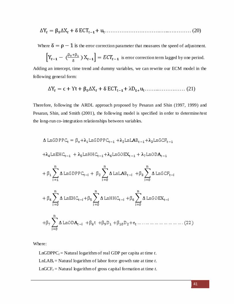
41
………………………….…...………… (20)
Where is the error correction parameter that measures the speed of adjustment.
is error correction term lagged by one period.
Adding an intercept, time trend and dummy variables, we can rewrite our ECM model in the
following general form:
……..…………… (21)
Therefore, following the ARDL approach proposed by Pesaran and Shin (1997, 1999) and
Pesaran, Shin, and Smith (2001), the following model is specified in order to determine/test
the long-run co- integration relationships between variables.
Where:
LnGDPPCt = Natural logarithm of real GDP per capita at time t.
LnLABt = Natural logarithm of labor force growth rate at time t.
LnGCFt = Natural logarithm of gross capital formation at time t.

42
LnEHC t = Natural logarithm of education human capital at time t.
LnHHC t = Natural logarithm of health human capital at time t.
LnGOEXt = Natural logarithm of total government expenditure at time t
LnODAt = Natural logarithm of official development assistance at time t.
are dummy variables for policy change and recurrent drought
, , , , , are coefficients that measure long run relationships.
, , , , , are coefficients that measure short run relationships.
is an error term and denotes lag length of the auto regressive process.
is the time trend of the model.
To test whether there is a long run equilibrium relationship between the variables; bounds test
for co- integration is carried out as proposed by Pesaran and Shin (1999) and Pesaran, Shin,
and Smith (2001). The hypotheses are shown below:
Ho: = means there is no long run
relationship among the variables.
Ha: means there is a long run
relationship among the variables.
The non-standard F-statistics is used to test the above hypothesis. The critical values of the F-
statistics for this test are available in Pesaran, Shin, and Smith (2001). On the other hand,
Narayan (2005) also estimated his own critical values by arguing that the critical values
provided by Pesaran, Shin, and Smith (2001) are appropriate for relatively large sample sizes.
He said that using such critical values for small sample size may produce misleading results.
As a result, Narayan (2005) has generated a new set of critical values for small sample sizes
ranging from 30 to 80 observations based on similar technique, GAUSS code6 , which was
employed by Pesaran, Shin, and Smith (2001). They provide two sets of critical values
namely the upper bound values and the lower bound values. If the computed F-statistics is
6 GAUSS code is a programming language designed for matrix-based operations and manipulat ions, suitable for
high level statistical and econometric computation.

43
higher than the appropriate upper bound of the critical value, the null hypothesis of no co-
integration will be rejected. If it is below the appropriate lower bound, the null hypothesis
cannot be rejected, and if it lies within the lower and upper bounds, the result would be
inconclusive. In this paper, the computed F-statistics is compared with both critical values
provided by Pesaran, Shin, and Smith (2001) and Narayan (2005.
After confirming the existence of long-run relationship among the variables, the following
stable long-run model is estimated:
The next step is to estimate the vector error correction model that indicates the short run
dynamic parameters (adjustment parameters that measure the speed of correction to long-run
equilibrium after a short-run disturbance). The standard ECM is estimated as follows:
……………………………………….……..…...(24)

44
Where:
, , , , , = coefficients that represents the short run dynamics of
the model .
= error correction term lagged by one period.
= vector of white noise error terms and denotes the optimal lag length of each
variable in the auto regressive process.
are dummy variables for policy change and recurrent drought
error correction parameter that measure the speed of adjustment towards the long run
equilibrium.
The error correction term term (ECT) is derived from the corresponding long run model
whose coefficients are obtained by normalizing the equation. After estimating the long run
and short run model, misspecification test, normality test, serial correlation test,
heteroscedasticity test and cumulative sum of recursive residuals (CUSUM) and the
cumulative sum of squares of recursive residuals (CUSUMSQ) test for stability of the model
is undertaken to check the robustness of the model. In order to estimate the models specified
in equation (22), (23) and (24) above and to perform the pre estimation and post estimation
diagnostic tests, Microfit4.1 and Eviews6 statistical packages are used.

45
CHAPTER FIVE
RESULTS AND DISCUSSION
5.1 Augmented Dicky-Fuller Unit Root Test
In order to determine the degree of stationarity, a unit root testing is carried out through the
standard Augmented Dicky-Fuller (ADF) test. This test was undertaken to check the order of
integration of the variables. The test was done for two alternative specifications. First it is
tested with constant but no trend, and then it is tested with constant and trend (See Table.3).
Table 3: ADF unit root test results
Source: Author’s Calculations.
Note: The rejection of the null hypothesis is based on MacKinnon (1996) critical values. Akaike informat ion
criterion (AIC) is used to determine the lag length while testing the stationarity of all variables. The ***, ** and
* sign indicates the rejection of the null hypothesis of non-stationary at 1%, 5% and 10% significant level
respectively
The results from this test show that six of the variables are non-stationary in their levels (for
both type of specifications) while the null of non-stationarity is not rejected for one variable
(health human capital- with intercept and trend) at 5 % level of significance .On the other
hand, in their first differences, all of the variables are stationary. These results indicate that,
with intercept and trend, six of the variables are I (1) and one of them is I (0). Such results of
Variables
(At level and 1st difference)
t-stat
( with intercept but no rend)
t-stat
(with intercept and trend )
LnLAB -2.3066 -1.9913
Δ LnLAB -5.7451*** -5.8121***
LnGCF -1.5491 -3.4126*
Δ LnGCF -4.3045*** -4.2318**
LnEHC -0.2712 -1.9382
Δ LnEHC -4.0889*** -3.9826**
LnHHC -1.1560 -4.2745***
Δ LnHHC -5.5383*** -5.4463***
LnGOEX -2.6037 -2.4077
Δ LnGOEX -4.6049*** -4.6030***
LnODA -1.3859 -2.0645
Δ LnODA -6.3378*** -6.3233***
LnGDPPC 0.3360 -0.5261
ΔLnGDPPC -4.5721*** -5.4292***

46
stationarity test would not allow us to apply the Johansen approach of co- integration. This is
one of the main justifications for using the ARDL approach (bounds test approach of
cointegration) developed by Pesaran, Shin, and Smith (2001).
5.2 Long run ARDL Bounds Tests For Co-integration
The first task in the bounds test approach of co- integration is estimating the ARDL model
specified in equation (22) using the appropriate lag- length selection criterion. In this paper
Akaike Information Criterion (AIC) was taken as a guide and a maximum lag order of 2 was
chosen for the conditional ARDL model. Then F-test through the Wald-test (bound test) is
performed to check the joint significance of the coefficients specified in equation (22). The
Wald test is conducted by imposing restrictions on the estimated long-run coefficients of real
GDP per capita, labor force growth, gross capital formation, education human capital, health
human capital, government expenditure and official development assistance. The computed
F-statistic value is compared with the lower bound and upper bound critical values tabulated
in Table CI (III) case IV of Pesaran, Shin, and Smith (2001) and Appendix-X case V of
Narayan (2005).
Table 4. Pesaran et al. (2001) and Narayan (2005) lower and upper bound critical value
Description
At 1% level At 5 % level
Lower
bound , I(0)
Upper
bound I(1)
Lower
bound I(0)
Upper
bound I(1)
Pesaran (2001) critical values for K=6 3.60 4.90 2.87 4.00
Narayan (2005) critical values for K=6 4.53 6.26 3.33 4.70
Source: Pesaran, Shin, and Smith (2001) and Narayan (2005) tables.
As it is depicted in Table-5 below, with an intercept and trend, the calculated F statistics 9.536
is higher than the Pesaran, Shin, and Smith (2001) and Narayan (2005) upper bound critical
values at 1% level of significance. This implies that the null hypothesis of
(there is no long-run relationship) against its alternative
(there is long-run relationship) is rejected based on the
Pesaran, Shin, and Smith (2001) and Narayan (2005) critical values at 1% level of
significance.

47
Table 5. Bounds test for co-integration analysis
Source: Author’s Calculations.
5.3 . Long-run Model Estimation.
This result indicates us the existence of a long-run relationship among real GDP per capita,
labor force, gross capital formation, education human capital, health human capital,
government expenditure and official development assistance. After confirming the existence
of long-run co- integration relationship among the variables, the estimated long-run
relationship between the variables are estimated and the estimated coefficients after
normalizing on real GDP per capita (GDPPC) are reported in Table 6.
Table 6. Estimated long run coefficients using the Autoregressive Distributed Lag
Approach :ARDL (1,0,2,2,2,2,1) selected based on Akaike Information Criterion
Dependent variable is LnGDPPC
Regressor Coefficients S.E T-Ratio Prob
LnLAB 0.09724 0.11326 0.8586 0.404
LnGCF -0.74489 0.37269 -1.9987 0.064
LnEHC 0.50965 0.14294 3.5656 0.003***
LnHHC 0.59292 0.21315 2.7817 0.014**
LnGOEX -0.45653 0.18191 -2.5096 0.024**
LnODA -0.17643 0.06854 -2.5740 0.021**
Policy change dummy(D1) 0.00804 0.10184 0.0790 0.938
Drought dummy (D2) -0.16527 0.04093 -4.0377 0.001***
Constant 4.22870 1.80160 2.3472 0.033**
Trend -0.01307 0.01871 -0.6987 0.495
Source: Author’s Calcu lations.
Note: The ***, ** and * sign indicates the significance of the coefficients at 1%, 5% and 10% significant level
respectively.
Description Value
Number of observation 37
Optimal Lag length of the model 2
Calculated F-statistic 9.536
R-Squared 0.98729 S.D. of Dependent Variable 0.23960
R-Bar-Squared 0.97118 Residual Sum of Squares 0.02482
S.E. of Regression 0.04068 Equation Log-likelihood 77.2398
F-stat. 61.305[0.000] Akaike Info. Criterion 57.2398
DW-statistics 2.1965 Schwarz Bayesian Criterion 41.6863
Mean of Dep. Variable 7.0529

48
As it is shown in Table-6, the estimated coefficients of labor force, health human capital and
education human capital, policy change dummy and drought dummy have the hypothesized
signs while gross capital formation, government expenditure and official development
assistance have unexpected signs. In addition, the estimated coefficients of education human
capital, health human capital, government expenditure, official development assistance, and
drought dummy are statistically significant while labor force, gross capital formation, and
policy dummy are not statistically significant.
Since I have specified my growth model in a log- linear form, the coefficient of the dependent
variable can be interpreted as elasticity with respect to real GDP per capita. The coefficient of
health is 0.5929. This indicates that, in the long run, holding other things constant, a one
percent change in health (proxied by the ratio of public health expenditure to GDP) brought
0.5929 percent change in real GDP. Next to health, education has significant long run impact
on the Ethiopian economy .A one percent increase in secondary school enrolment has resulted
in 0.5096 percent change in real GDP per capita. The findings of this research concerning the
long run positive impact of the education and health human capital are consistent with the
endogenous growth theories (mainly advocated and/or developed by Lucas (1988) , Romer
(1990), Mankiw, Romer and Weil (1992)) which argue that improvement in human capital
(skilled and healthy workers) leads to productivity improvement that enhances output. With
respect to the researches made in Ethiopia, the finding of this research is also similar to
Teshome (2006) and Tofik (2012).
On the other hand, government expenditure and official development assistance and drought
have a significant negative impact to the Ethiopian economy. The significant negative impact
of government expenditure on the Ethiopian economy is consistent with the findings of Tofik
(2012) and Teshome (2006) entailing the dominance of the unproductive and inefficient
government spending that could not add any value to the economy (like wages and salaries,
rent, debt servicing and transfer payments). The finding of this research in relation to ODA is
also similar to the findings of Rajan and Subramanian (2005), Ekanayake and Chatrna (2008),
Mallik (2008), and Tasew (2011). Labor force growth has no any significant impact on real
GDP per capita. This may be due to the combined effect of high population growth and low
productivity of the labor force. Further, the unexpected sign of gross capital formation is

49
similar to the findings of Martha (2008) and Tadesse (2011). The unexpected sign of the
coefficient of GCF contradicts with economic growth theories. In my opinion, it may be data
and/or valuation problem, but it is difficult to justify the exact reason behind such unexpected
result using this research. Hence, further detailed research should be done to identify the
reason behind such result (unexpected sign of GCF).
5.3.1 Long-run diagnostic tests
To check the verifiability of the estimated long run model, some diagnostic test is undertaken.
The results reported in Table-7 indicate that there is no error autocorrelation and
heteroskedasticity, and the errors are normally distributed. In addition the Ramsey functional
form test confirms that the model is specified well .Hence, the relationship between the
variables is verifiable or valid.
Table 7. Long-run diagnostic tests
Test Statistics LM Version F Version
Serial Correlation test CHSQ(1)= 0.58187[0.446]** F(1, 14) = 0.23668[0.634]**
Functional Form test CHSQ(1)= 1.06340[0.302]** F(1, 14) = 0.43869[0.519]**
Normality test CHSQ(2)= 0.79174[0.673]** Not applicable Heteroscedasticity test CHSQ(1)= 0.00974[0.921]** F(1, 33) = 0.00919[0.924]**
Source: Author’s Calcu lations.
Note: The sign ** indicates the significance of the coefficients at 5% level of significance. The test for serial
correlation is the LM test for autocorrelation, the test for functional form is Ramsey’s RESET test, the test for
normality is based on a test of skewness and kurtosis of residuals, the test for heteroskedasticity is based on the
regression of squared residuals on squared fitted values .
In addition to the above diagnostic tests, the stability of long run estimates has been tested by
applying the cumulative sum of recursive residuals (CUSUM) and the cumulative sum of
squares of recursive residuals (CUSUMSQ) test. Such tests are recommended by Pesaran and
Shin (1999, 2001).
Since the test statistics of this stability tests can be graphed, we can identify not only their
significance but also at what point of time a possible instability (structural break) occurred. If
the plot of CUSUM and CUSUMSQ statistic moves between the cr itical bounds (at 5%
significance level), then the estimated coefficients are said to be stable.

50
Fig 5. Plot of cumulative sum of recursive residuals
Source: Author Calculat ions.
Note: The straight lines represent critical bounds at 5% significance level
Fig 6. Plot of cumulative sum of squares of recursive residuals
Source: Author Calculat ions.
Note: The straight lines represent critical bounds at 5% significance level
-0.5
0.0
0.5
1.0
1.5
1977 1979 1981 1983 1985 1987 1989 1991 1993 1995 1997 1999 2001 2003 2005 2007 2009 2011
-5
-10
-15
0
5
10
15
1977 1979 1981 1983 1985 1987 1989 1991 1993 1995 1997 1999 2001 2003 2005 2007 2009 2011

51
The results of both CUSUM and CUSUMSQ test are reported in Figures 5 and 6 . As can be
seen from the first figure, the plot of CUSUM test did not cross the critical limits. Similarly,
the CUSUMSQ test shows that the graphs do not cross the lower and upper critical limits. So,
we can conclude that long and short runs estimates are stable and there is no any structural
break. Hence the results of the estimated model are reliable and efficient.
5.4 . Short run Error Correction Estimates
After the acceptance of long-run coefficients of the growth equation, the short-run ECM
model is estimated. The coefficient of determination (R-squared) is high explaining that about
90.235 % of variation in the real GDP is attributed to variations in the explanatory variables in
the model. In addition, the DW statistic does not suggest autocorrelation and the F-statistic is
quite robust.
The equilibrium error correction coefficient, estimated -0.7366 is highly significant, has the
correct sign, and imply a very high speed of adjustment to equilibrium after a shock.
Approximately 73.66 percent of the disequilibrium from the previous year’s shock converges
back to the long-run equilibrium in the current year. Such highly significant Error correction
term is another proof for the existence of a stable long run relationship among the variables
(Banerjee, et al., 2003).
The estimated short-run model reveals that education is the main contributor to real GDP per
capita change followed by gross capital formation (one period lagged value) and government
expenditure (one period lagged value). When enrolment increases by one percent, real GDP
per capita increases by 0.76867 percent while the same percentage change in its one period
lagged value resulted in about 0.7150 percent rise in real GDP per capita. But, unlike its long
run significant impact, health has no significant short run impact on the economy. Even its
one period lagged value has a significant negative impact on the economy. This could be due
to the reason that health expenditure may have big impact on the people who have no positive
impact on the economy. Due to this, it may increase the dependency ratio that dilutes
resources of the economy that would have been invested in creating new assets and values.
The other possible reason could be high rate of unemployment. That means, even though

52
health status of the labor force increases in the short run, until it is employed it will dilute
resources that would have been allocated for new investment.
Table 8. Error correction representation for the selected Autoregressive Distributed
Lag model : ARDL (1,0,2,2,2,2,1) selected based on Akaike Information Criterion
Source: Author’s Calcu lations.
Contrary to its insignificant long run impact, one period lag of gross capital formation has a
positive contribution to economic growth at 5 percent level. Similarly, a one period lagged
value of government expenditure has a positive impact on real GDP per capita. In addition,
Dependent variable is ΔLnGDPPC
Regressor Coefficients S.E T-Ratio Prob
ΔLnLAB 0.07163 0.09103 0.7869 0.441
ΔLnGCF 0.11542 0.07965 1.4492 0.163
ΔLnGCF(-1) 0.31605 0.10660 2.9648 0.008***
ΔLnEHC 0.76867 0.21877 3.5136 0.002***
ΔLnEHC(-1) 0.71501 0.22209 3.2194 0.004***
ΔLnHHC -0.06594 0.07250 -0.9095 0.374
ΔLnHHC(-1) -0.18325 0.08123 -2.2560 0.035**
ΔLnGOEX -0.10862 0.13065 -0.8314 0.416
ΔLnGOEX(-1) 0.25814 0.10822 2.3854 0.027**
ΔLnODA -0.03819 0.05875 -0.6501 0.523
Policy change Dummy(D1) 0.00593 0.07500 0.0790 0.938
Drought Dummy(D2) -0.12174 0.02871 -4.2405 0.000***
Constant 3.11490 1.58110 1.9701 0.063*
Trend -0.00963 0.01465 -0.6573 0.518
ECM(-1) -0.73660 0.19218 -3.8329 0.001*** Where , ECM = RGDP-0.097240*LAB+ 0.74489*PCAP-0.50965*EHC-0.59292*HHC +0.45653*GOEX
+0.17643*ODA -0.0080438* D1 + 0 .16527* D2 -4.2287* constant + 0.013072*Trend
R-Squared 0.90235 S.D. of Dependent Variable 0.08646
R-Bar-Squared 0.77867 Residual Sum of Squares 0.02482
S.E. of Regression 0.04068 Equation Log-likelihood 77.2398
F-stat. 9.9013[0.000] Akaike Info. Criterion 57.2398
DW-statistics 2.19650 Schwarz Bayesian Criterion 41.6863
Mean of Dep. Variable 0.01314

53
unlike its negative long run effect, official development assistance has no significant effect on
the economy in the short run.
5.4.1 Short-run diagnostic tests
To check the verifiability of the estimated short run model, some diagnostic test is
undertaken. The results reported in Table-9 indicate that there is no error autocorrelation and
heteroskedasticity, and the errors are normally distributed. In addition the Ramsey functional
form test confirms that the model is specified well .Hence, the relationship between the
variables is verifiable or valid.
Table 9.Short run diagnostic test
Test Statistics LM Version F Version
Serial Correlation test CHSQ(1)= 0.07801[0.780]** F(1, 19) = 0.04244[0.839]**
Functional Form test CHSQ(1)= 1.17343[0.279]** F(1, 19) = 0.64780[0.431]**
Normality test CHSQ(2)= 0.72033[0.688]** Not applicable
Heteroscedasticity test CHSQ(1)= 16.55290[0.281]** F(1, 33) = 1.28188[0.299]**
Source: Author’s Calcu lations.
Note: The sign ** indicates the significance of each diagnostic tests at 5% level of significance. The test for
serial correlation is the LM test for autocorrelation, the test for functional form is Ramsey’s RESET test, the test
for normality is based on Jarque-bera test, and the test for heteroskedasticity is based on Breusch-Pagan-Godfrey
test.
5.5 The Pair wise Granger Causality Results
A granger causality test is made to identify the direction of causality between the dependent
variable, education and health. The result is reported in Table-10 below. The result revealed
that, at lag length of one, there is significant causality between real GDP per capita, education
human capital (proxied by secondary school enrolment) and health human capital (proxied by
the ratio of public health expenditure to real GDP).

54
Table 10. Pair wise granger causality test
Null Hypothesis
Lag length 1 Lag length 2
F-stat Prob. F-stat Prob.
EHC does not Granger Cause GDPPC 5.89901 0.0208** 2.22794 0.1253
GDPPC does not Granger Cause EHC 12.9837 0.0010*** 1.64900 0.2092
HHC does not Granger Cause GDPPC 3.91545 0.0056*** 1.97634 0.1562
GDPPC does not Granger Cause HHC 0.54944 0.4638 2.42323 0.1058
Source: Author’s Calcu lations.
Note: The signs *** and ** indicate the significance of the coefficients at 1% and 5% level of significance
respectively.
There is a Uni-directional causal relationship from health to real GDP per capita while a Bi-
directional relationship is identified between real GDP per capita and education. The
bidirectional relationship between real GDP per capita and education implies that education
(secondary school enrolment) is not only a cause for real GDP per capita change but it is also
an effect. On the other hand, when the lag length of the ARDL model increases to two, there
is no any significant causality between real GDP per capita, education human capital and
health human capital.
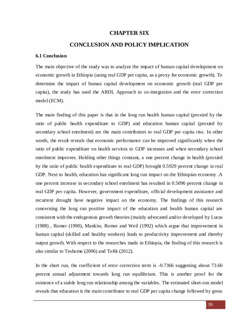
55
CHAPTER SIX
CONCLUSION AND POLICY IMPLICATION
6.1 Conclusion
The main objective of the study was to analyze the impact of human capital development on
economic growth in Ethiopia (using real GDP per capita, as a proxy for economic growth). To
determine the impact of human capital development on economic growth (real GDP per
capita), the study has used the ARDL Approach to co-integration and the error correction
model (ECM).
The main finding of this paper is that in the long run health human capital (proxied by the
ratio of public health expenditure to GDP) and education human capital (proxied by
secondary school enrolment) are the main contributors to real GDP per capita rise. In other
words, the result reveals that economic performance can be improved significantly when the
ratio of public expenditure on health services to GDP increases and when secondary school
enrolment improves. Holding other things constant, a one percent change in health (proxied
by the ratio of public health expenditure to real GDP) brought 0.5929 percent change in real
GDP. Next to health, education has significant long run impact on the Ethiopian economy .A
one percent increase in secondary school enrolment has resulted in 0.5096 percent change in
real GDP per capita. However, government expenditure, official development assistance and
recurrent drought have negative impact on the economy. The findings of this research
concerning the long run positive impact of the education and health human capital are
consistent with the endogenous growth theories (mainly advocated and/or developed by Lucas
(1988) , Romer (1990), Mankiw, Romer and Weil (1992) which argue that improvement in
human capital (skilled and healthy workers) leads to productivity improvement and thereby
output growth. With respect to the researches made in Ethiopia, the finding of this research is
also similar to Teshome (2006) and Tofik (2012).
In the short run, the coefficient of error correction term is -0.7366 suggesting about 73.66
percent annual adjustment towards long run equilibrium. This is another proof for the
existence of a stable long run relationship among the variables. The estimated short-run model
reveals that education is the main contributor to real GDP per capita change followed by gross

56
capital formation (one period lagged value) and government expenditure (one period lagged
value). When enrolment increases by one percent, real GDP per capita increases by 0.7686
percent while the same percentage change in one period lagged value of it resulted in about
0.7150 percent rise in real GDP per capita. But, unlike its long run significant impact, health
has no significant short run impact on the economy. Even its one period lag has a significant
and negative impact on the economy. This could be due to the reason that health expenditure
may have big impact on the people who have no positive impact on the economy. As a result,
dependency ratio may increase that dilute resources of the economy that would have been
invested in creating new assets and values.
A causality test result indicates that there is a Uni-directional causal relationship from health
to real GDP per capita while a Bi-directional relationship is identified between real GDP per
capita and education. On the other hand, when the lag length of the VAR increases to two,
there is no any significant causality between real GDP per capita, education human capital
and health human capital.
6.2 Policy Implication
The results of this study have important policy implications. In order to improve economic
growth, public expenditure needs to be better prioritized towards basic health service
provision. In addition, to achieve economic growth, more resources should be devoted to
educate the citizens of the country. Such measures have a large impact on human productivity
which leads to improved national output per capita. In other words, as more people become
educated and healthy, they will increase their productivity in the long run. Although not
investigated in this paper, one of the ways through which education and health affects
economic wellbeing is its externalities effect. That means, education and health may have
indirect benefits (positive spillovers) that enhance productivity in the long run.
Hence policy makers and / or the government should strive to create institutional capacity that
increase school enrolment and improve basic health service. That means, the policy makers
and the government should center on securing more resources and structures that are essential
and appropriate for better school enrolment and improved basic health service provision. Such
measures should focus not only on creating new institutional capacity, but also on
57
strengthening and changing the existing institutional setups of the education and health
sectors of Ethiopia that produce quality manpower. In addition, the government should also
continue its leadership role in creating enabling environment that encourage better investment
in education and health by the private sector. Because, healthier participation of the private
sector in the education and health sectors can speed up the creation of human capital in
Ethiopia.

REFERENCE
Adams, S. (2009). Can Foreign Direct Investment Helps to Promote Growth in Africa? African Journal of Business Management, 3 (5):78-183.
Aghion, P. and P. Howitt (2009). The Economics of Growth. Cambridge, Massachusetts: The
MIT Press.
Ang, J.B. (2007). Financial Deepening and Economic Growth in Malaysia. Asian Business and
Economics Research Unit Discussion Paper No 42. Caulfield, Australia: Department of Economics, Faculty of Business & Economics, Monash University,
Appleton, S. and F. Teal (1998).Human Capital and Economic Development. A Background Paper Prepared for the African Development Report.
Baldwin, N. and S. Borrell (2008). Education and Economic Growth in the United States: Cross-
National Applications for an Intra-national Path Analysis. Policy Science, 41: 183-204.
Barro, R.J (1991). Economic Growth in a Cross Section of Countries. Quarterly Journal of
Economics, 106(2): 407-443. Barro, R. (1996). Health and Economic Growth. Mimeo, Cambridge: Harvard University.
Barro, R. (2013).Health and Economic Growth. Analysis of Economics and Finance, 14(2): 329-
366. Barro, R.J, (2003).Determinants of Economic Growth in a Panel of Countries. Analysis of
Economics and Finance, 4:231–274.
Barro, R.J and J. Lee (2000).International Data on Educational Attainment: Updates and Implications . NBER Working Paper No 7911. Cambridge, Massachusetts.
Barro, R.J, and J. Lee (2010) .A new Data Set of Educational Attainment in the World, 1950-2010: NBER Working Paper No 15902. Cambridge, Massachusetts.
Barro, R.J and X. Sala-i-Martin (1995). Economic Growth. New York: McGraw-Hill.
Barro, R.J. and X. Sala- i-Martin (2004). Economic Growth. 2nd Edition, Cambridge, Massachusetts, London, England: The MIT Press.
Banerjee, A., Dolado, J., Galbraith, J., and D. Hendry (2003).Co-integration, Error Correction,
and the Econometric Analysis of Non-stationary Data: Advanced Text in Econometrics.
New York: Oxford university press.
Bassanini, A. and S. Scarpetta (2001). Does Human Capital matter for growth in OECD Countries? Evidence from pooled mean-group estimates. OECD Economics Department Working papers No 282: OECD Publishing.

Basov, S. (2002). Heterogeneous Human Capital: Life Cycle Investment in Health and Education. University of Melbourne, Victoria, Australia.
Becker, G. (1962). Investment in Human Capital: A Theoretical Analysis. Journal of Political
Economy ,70(5): 9-49. Becker, G. S (1993). Human Capital: A Theoretical and Empirical Analysis with Special
Reference to Education. 3rd edition, Chicago and London: University of Chicago Press.
Benhabib, J. and M. Spiegel (2002).Human Capital and Technology Diffusion: FRBSF Working Paper No 2003-02. New York University and Federal Reserve Bank of San Francisco
Bergheim, S. (2005). Human Capital is The Key to Growth: Success stories and policies for 2020. Deutsche Bank AG, Dutch Bank Research, Frankfurt am Main, Germany.
Bernanke, B. and R. Gurkanak (2001). Is Growth Exogenous? Taking Mankiw, Romer, and Weil Seriously. National Bureau of Economic Research working paper series No 8365.
Massachusetts, Cambridge.
Bloom, D., Canning, D.and J. Sevilla (2004). The Effect of Health on Economic Growth: A Production Function Approach, World Development, 32(1):1-13.
Cass, D (1965). Optimum Growth in an Aggregative Model of Capital Accumulation. The Review of Economic Studies, 32(3):233-240.
Chaudhry, M. and M. Choudhary (2006).Why the State Bank of Pakistan should not Adopt
Inflation Targeting. SBP-Research Bulletin, 2(1):196-2009.
Christian, M. (2011). Human Capital Accounting in the United States: Context, Measurement,
and Application , Wisconsin Center for Education Research ,Madison, USA. CSLS (2001). The Development of Indicators for Human Capital Sustainability: Centre for the
Study of Living Standards. Paper prepared for the CSLS session at the annual meeting of the Canadian Economics Association, McGill University, Montreal, Canada.
Dae-Bong, K.(2009). Human capital and its Measurement: The 3rd OECD World Forum on
Statistics, Knowledge and Policy” Charting Progress, Building Visions, Improving Life.
Busan, Korea.
De Pleijt, A.M (2011). The Role of Human Capital in the Process of Economic Development: The Case of England. Center for Global Economic History Working Paper Series No 21: Center for Global Economic History.
Diewert, E. (2008). The Measurement of Nonmarket Sector Outputs and Inputs Using Cost
Weights. Discussion Paper No 08-03, Department of Economics, University of British, Columbia, Vancouver, B.C. Canada.

Dorwick, S. (2003). Ideas and Education: Level or Growth Effects? NBER Working Paper No 9709, Massachusetts ,Cambridge.
Duma, N. (2007). Sri Lanka’s Sources of growth. IMF working paper No. 07/225.
Easterly, W, (1993). How Much Do Distortions Affect Growth? Journal of Monetary
Economics, 32(2):187–212.
EEA/EEPRI (2010). Ethiopian economic association database, EEA, Addis Ababa.
Eisner, R. (1988). Extended accounts for national income and product. Journal of Economic Literature , 26 (4): 1611-1684.
Ekanayake, E.M and D. Chatrna (2008). The Effect of Foreign Aid on Economic Growth in Developing Countries. Journal of International Business and Cultural Studies:1-13
Enders ,W.(1996). Applied Econometric Time Series. Lowa State University: John Wiley & Sons
INC.
Evans, R., Barer, M. and T. Marmor (1994). Why Are Some People Healthy and Others Not?
The Determinants of Health of Populations, New York, Aldine de Gruyter : 378. Fleischhauer, K. (2007). A Review of Human Capital Theory: Microeconomics. Discussion
Paper No 2007-01: Department of Economics, University of St. Gallen, Bodanstrasse.
Gardner, H and D. Gardner (2001). Health as Human Capital: Theory and Implications .A New Management Paradigm, HCMS Group .Available at: < http://www.hcmsgroup.com/wp- content/uploads/2012/05/WP01-HHC> (accessed on December 22, 2012).
Goldsteine, M., and M. Khan (1976). Large versus Small Price Changes and the Demand for
Imports. International Monetary Fund, 23(1): 200-225. Green, H.M (2004).Econometric Analysis. New York University: Prentice hall, upper Saddle
River, New Jersey.
Gu, W. and A. Wong (2010). Investment in Human Capital and the Output of the Education Sector in Canada: Paper Prepared for the 31st General Conference of the International Association for Research in Income and Wealth Economic Analysis, St.Gallen,
Switzerland..
Gujarati. (2004). Basic econometrics. McGraw-Hill Companies, 4th edition. Gundlach, E. (1996). Human capital and economic development: A Macroeconomic Assessment.
Kieler Arbeitspapiere Working paper No 778. ECONSTOR, The Open Access Publication Server of the ZBW – Leibniz Information Centre for Economics.

Gyimah-Brempong, K. and M. Wilson (2005). Human Capital and Economic Growth. Is Africa Different? Journal of African Development, 7(1): 73-109.
Hansen, H. and F. Tarp (2000). Aid and Growth Regressions, CREDIT Research Paper No 00/7.
University of Nottingham, UK: Centre for Research in Economic Development and International Trade,
Hanushek, E and L. Wobmann (2007).The Role of Education Quality in Economic Growth. World Bank Policy Research Working Paper 4122.
Harbison, F.H (1971). Human Resources as the Wealth of Nations. Proceedings of the American
Philosophical Society, 115(6):426-431.
Harris, R.(1999).Using Co-integration Analysis in Econometric Modeling. London, Prentice hall.
Harris, R. and R. Sollis (2003). Applied Time Series Modeling and Forecasting. Durham
University, West Essex, England : John Wiley & Sons Ltd .
Howitt, P. (2005). Health, Human capital and Economic growth: A Schumpeterian perspective.
Paper Prepared for the Pan American Health Organization, Washington, DC. ILO. (2003).Learning and Training for Work in the Knowledge Society: The constituents’ views.
International Labour Office Report IV, Geneva, Switzerland, ISBN 92-2-112877-6, ISSN 0074-6681.
Jones, R. and V. Fender (2011). Human Capital Estimates of 2010. Office for National Statistics, UK
Karagiannis, S. and K. Benos (2009). The Role of Human Capital in Economic Growth: Evidence from Greek Regions. Centre for Planning and Economic Research No 105,
Athens, Greece.
Kefela, G. and R. Rena (2007). Human Capital Investment Is a Continuous Proposition: A Study of North East African States. Indus Journal of Management & Social Sciences, 2(1):54-70.
Kendrick, J.W (1976). The Formation and Stocks of Total Capital. National Bureau of Economic Research No 100. New York and London: NBER Inc.
Kern, A.F.(2009). Human Capital Development Theory: Implications for Education: Comparison of Influential Twenty-First Century Economists Samuel Bowles and Gary S. Becker:
Available at: < http://www.personal.psu.edu/afk119/blogs/career_tech_ed/2009/12/human- capital-development > (accessed on December 1,2012).
Le, T., Gibson,J., and L. Oxley, (2003). Cost and income based measures of human capital:
Journal of Economic Surveys, 17(3): 271–307.

Levine, R. and D. Renelt (1992). A Sensitivity Analysis of Cross-country Growth Regressions. The American Economic Review, 82(4): 942-963.
Lucas, R.(1988). On the Mechanics of Economic Development.Journal of Monetary Economics,
22(1988):3- 42. Madsen, B. Saxena ,S. and B. Ang (2008). The Indian Growth Miracle and Endogenous Growth.
Discussion paper No17/08. Department of Economics, Monash University of Business and Economics.
Mallik, G.(2008). Foreign Aid and Economic Growth: A Co- integration Analysis of the Six
Poorest African Countries. Economic Analysis & Policy, 38(2): 2.251-260
Mankiw, G., Romer, D. and N. Weil (1992). A Contribution to the Empirics of Economic
Growth. Quarterly Journal of Economics, 107 (2): 407-437.
Marimuthu, M., Arokiasamy, L. and M. Ismail (2009). Human Capital Development and Its Impact on firm’s Performance: Evidence from Developmental Economics. The Journal of
International Social Research, 2(80): 266-272. Martha, H.(2008). Productivity and Human Capital: The case of Ethiopia. Unpublished Masters
Thesis. Oslo University, Oslo, Norway.
McMahon, W. (1998). Education and Growth in East Asia. Economics of Education Review, 17(2) : 159-172
McMahon, W.(2010).The Private and Social Benefits of Higher Education : The Evidence ,Their Value, and Policy Implications, University of Illinois at Urbana-Champaign: TIAA- REF
Institute. Mincer, J.(1981).Human Capital and Economic Growth. National Bureau of Economic Research,
Working Paper No 803 , Massachusetts avenue, Cambridge.
Mincer, J.(1989). Human capital responses to technological change in the labor market, Proceedings of a Conference on Economic Growth at Suny, Buffalo, New York.
Mincer, J. (1996). Economic Development, Growth of Human Capital, and the Dynamics of the Wage Structure. Journal of Economic Growth ,1(1): 29-48
MoE. (2008). National Report of the Federal Democratic Republic of Ethiopia: Development of
Education and Inclusive Education. Ministry of Education, Addis Ababa, Ethiopia.
MoE. (2010). Health Sector Development Programme IV: Final draft. Ministry of Education,
Addis Ababa, Ethiopia. Mongabay. (2010). Ethiopia-Eduction , Available at : < http://www.mongabay.com/history/
ethiopia/ethiopia-health_and_welfare.html> (accessed on November 22, 2012).
Moretti, E. (2006).Private and Social Returns to Education. Rivista Dipolitica Economica, Maggio-GIugno.
Mulligan, C. and X. Sala-I-Martin (2000). Measuring Aggregate Human Capital. Journal of
Economic Growth, 5(3): 215-252. Narayan, P. (2005). The Saving and Investment Nexus for China: Evidence from Co-integration
Tests .Applied Economics, 37: 1979-1990.
Odior, E.S (2011). Government Expenditure on Health, Economic Growth and Long Waves in A CGE Micro-Simulation Analysis: The Case of Nigeria. European Journal of Economics Finance and Administrative Sciences, 3(2011):101-113.
Oluwatobi, S. & I. Ogunrinola (2011).Government Expenditure on Human Capital Development:
Implications for Economic Growth in Nigeria. Journal of Sustainable Development, 4(3):72-80.
Oumer, J.( 2007). The Challenges of Free Primary Education in Ethiopia. International Institute for Educational Planning (IIEP), Paris, France.
Qadri, F. and A. Waheed (2011). Human Capital and Economic Growth: Time Series Evidence
from Pakistan. Pakistan Business Review ,1: 815-833.
Patron, R. ( 2006). Trade, Education and Skills: A Theoretical Survey. Documento No 10/06.
dECON, Universidad de la República, Uruguay. Pesaran, H. and Y. Shin (1997).An Autoregressive Distributed Lag Modeling Approach to Co-
integration Analysis, Cambridge, England.
Pesaran, H. and Y. Shin (1999).An Autoregressive Distributed Lag Modeling Approach to Co-integration Analysis, Cambridge, England.
Pesaran, H., Shin,Y.,and R. Smith (2001). Bounds Testing Approaches to the Analysis of Level Relationships. Journal of Applied Econometrics, 16(3):1924-1996.
Rahimi, M. and A. Shahabadi (2011). Trade Liberalization and Economic Growth in Iranian
Economy, Bu-Ali Sina University, Hamedan, Iran. Available at: < http://ssrn.com/abstract
> (accessed on February 25 ,2013)
Rajan, R. and A. Subramanian (2005). Aid and Growth: What Does the Cross-Country Evidence Really Show? International Monetary Fund Working Paper No 05/127.
Romer, P.(1990). Endogenous Technical Change. The Journal of Political Economy, 98(5): S71-S102.
Sankay, O. Ismail, R. and A. Shaari (2010). The Impact of Human Capital Development on the
Economic Growth of Nigeria. Prosiding Perkem V, ISSN: 2231-962X: 63-72.

Sarmad, K.(1988). The Functional Form of the Aggregate Import Demand Equation: Evidence
from Developing Countries. The Pakistan Development Review, 27(3): 309-315.
Seid , N. (2000). The Determinants of Economic Growth in Ethiopia, Msc. Unpublished Thesis, School of Graduate Studies, A.A.U, Ethiopia.
Schultz, T.W (1961). Investment in Human Capital. American Economic Review, 51(1): 1-17.
Schreyer, P. (2010). Towards Measuring the Volume Output of Education and Health Services: A hand book OECD Statistics Working Papers No 2010/02, OECD Publishing, Available at: < http://dx.doi.org/10.1787/5kmd34g1zk9x-en > (Accessed on March 11, 2013)
Solow, R.M (1956). A contribution to the Theory of Economic Growth. Quarterly Journal of
Economics, 70(1): 65-94. Spence, M.(1973). Job market signaling. Quarterly Journal of Economics, 87(3) :355-375.
Ssekuma, R.(2012). A study of Co- integration Models with Applications, University of South
Africa. Strauss, J. and D. Thomas (1998). Health, Nutrition, and Economic Development. Journal of
Economic Literature, 36(2) : 766-817.
Tadese,D.B.(2011). Sources of Economic Growth in Ethiopia.A Time Series Empirical Analysis. Unpublished Master’s Thesis, Department of Economics, University of Oslo, Oslo.
Tasew, T. (2011). Foreign Aid and Economic Growth in Ethiopia: A Co-integration Analysis. The Economic Research Guardian, 1(2):88-108.
Teshome, K. (2006). The impact of government spending on economic growth: the case of
Ethiopia: unpublished thesis, Addis Ababa University, Addis Ababa, Ethiopia.
Tofik, S. (2012). Official Development Assistance (ODA), Public Spending and Economic
Growth in Ethiopia. Journal of Economics and International Finance, 4(8):173-191. Udoh, E. and U. Ogbuag (2012). Financial Sector Development and Industrial Production in
Nigeria (1970-2009): An ARDL Co-integration Approach .Journal of Applied Finance & Banking, 2 (4): 49-68.
UNDP. (2011). Human Development Report: Sustainability and Equity: A Better Future for All.
The United Nations Development Programme, UN Plaza, New York, USA.
UNESCO. (2010). UNESCO Institute for Statistics Data base , Available at www.uis.unesco.org
(accessed on November 22).

Umaru, A. (2011). Human Capital: Education and Health in Economic Growth and Development of the Nigerian. British Journal of Economics, Finance and Management Sciences, 2(1):
22-36.
Viste, E., Korecha, D., and A. Sorteberg (2012). Recent Drought and Precipitation Tendencies in Ethiopia. Theor Appl Climatol, 112: 535–551.
WDE. (2010). World Data on Education.7th Edition, UNESCO-IBE.
Webb, P., Braun, J. and Y. Yisehac (1992).Famine in Ethiopia: Policy Implications of Coping
Failure at National and Household level .Research Report number 92: International Food Policy Research Institute, Washington DC.
Weil, N. (2009). Economic growth. 2nd edition, Prentice Hall publishing, New Jersey, USA.
Wilson, R. and G. Briscoe (2004).The Impact of Human Capital on Economic growth: A review on the Impact of Education and Training: Third Report on Vocational Training Research in Europe: Office for Official Publications of the European Communities, Luxembourg.
World Bank. (2011). World Bank National Accounts Data and OECD National Accounts data
Files, Available at: < http://data.worldbank.org/indicator/NY.GDP (accessed on Jan ,2013). Woubet, K. (2006). Human Capital and Economic Growth in Ethiopia: Unpublished Master’s
Thesis, Addis Ababa University, Addis Ababa, Ethiopia, pp.22.
Xiao, J. (2001). Determinants of Salary Growth in Shenzhen, China: An analysis of Formal Education, On-the-Job Training, and Adult Education with a Three- level Model. The China Review, 1(1): 73–110.
Yaffee, R. (1999). Introduction to Time Series Analysis and Forecasting: With Applications of
SAS and SPSS. New York : Academic press.
Zarra-Nazhad, M. and F. Hosainpour (2011). Review of Growth Models in Less Developed
Countries. The International Journal of Applied Economics and Finance, 5(1): 1-17.

ANNEX
R-Squared 0.98729 S.D. of Dependent Variable 0.23960
R-Bar-Squared 0.97118 Residual Sum of Squares 0.02482
S.E. of Regression 0.04068 Equation Log-likelihood 77.2398
F-stat. 61.3046[.000] Akaike Info. Criterion 57.2398
DW-statistics 2.1965 Schwarz Bayesian Criterion 41.6863
Mean of Dep. Variable 7.0529
Diagnostic tests
Test Statistics LM Version F Version
Serial Correlation test CHSQ(1)= 0.58187[0.446]** F(1, 14) = 0.23668[0.634]**
Functional Form test CHSQ(1)= 1.06340[0.302]** F(1, 14) = 0.43869[0.519]**
Normality test CHSQ(2)= 0.79174[0.673]** Not applicable Heteroscedasticity test CHSQ(1)= 0.00974[0.921]** F(1, 33) = 0.00919[0.924]**
Source: Author’s Calcu lations.
Table-A. Autoregressive Distributed Lag estimates (Dynamic estimation Results)
ARDL(1,0,2, 2,2,2,1) selected based on Akaike information Criterion
Dependent variable is LnGDPPC
Regressor Coefficient Standard Error T-Ratio Prob
LnGDPPC(-1) 0.2634 0.1922 1.3706 0.191
LnLAB 0.0716 0.0910 0.7869 0.444
LnGCF 0.1154 0.0797 1.4492 0.168
LnGCF(-1) -0.3481 0.1221 -2.8501 0.012**
LnGCF (-2) -0.3161 0.1066 -2.9648 0.010***
LnEHC 0.7687 0.2188 3.5136 0.003***
LnEHC(-1) 0.3218 0.2214 1.4534 0.167
LnEHC(-2) -0.7150 0.2221 -3.2194 0.006***
LnHHC -0.0659 0.0720 -0.9095 0.377
LnHHC(-1) 0.3194 0.1120 2.9878 0.011**
LnHHC(-2) 0.1833 0.0812 2.2560 0.039**
LnGOEX -0.1086 0.1307 -0.8314 0.419
LnGOEX(-1) 0.0305 0.1177 0.2591 0.799
LnGOEX(-2) -0.2581 0.1082 -2.3854 0.031**
LnODA -0.0382 0.0586 -0.6501 0.525
LnODA(-1) -0.0918 0.0673 -1.3636 0.193
Policy change dummy(D1) 0.0059 0.0750 0.0790 0.938
Drought dummy (D2) -0.1217 0.0287 -4.2405 0.001***
Conctant -3.1149 1.5811 1.9701 0.068*
Trend -0.0096 0.0147 -0.6573 0.521

Table-B. Estimated model for Wald test (Bound test)
Dependent Variable: Δ (GDPPC)
Method: Least Squares, Included observations: 34 after adjustments
Variables Coefficient Std. Error t-Statistic Prob.
GDPPC(-1) -1.104085 0.228872 -4.824025 0.0170 GCF(-1) -2.160438 0.560328 -3.855665 0.0308
LAB(-1) 0.057786 0.128485 0.449748 0.6834 HHC(-1) 0.939590 0.302394 3.107171 0.0530 EHC(-1) 1.094549 0.220404 4.966099 0.0157
ODA(-1) 0.043176 0.083182 0.519051 0.6396 GOEX(-1) 0.214299 0.287374 0.745713 0.5100
Δ(PCAP) 0.201688 0.074389 2.711273 0.0731 Δ (LAB) 0.322890 0.120570 2.678029 0.0752 Δ (EHC) 1.554877 0.248026 6.268996 0.0082
Δ (HHC) -0.011941 0.060132 -0.198583 0.8553 Δ (ODA) -0.097219 0.056548 -1.719236 0.1841
Δ (GOEX) 0.545869 0.179531 3.040525 0.0558 Δ (GDPPC(-1)) -0.586560 0.246184 -2.382608 0.0974
Δ (GCF(-1)) 1.607739 0.424163 3.790379 0.0322
Δ (LAB(-1)) 0.253491 0.074404 3.406950 0.0422 Δ (HHC(-1)) -0.505216 0.168145 -3.004638 0.0575
Δ (EHC(-1)) 1.145734 0.269748 4.247425 0.0239 Δ (ODA(-1)) -0.391221 0.113192 -3.456257 0.0408
Δ (GOEX(-1)) 0.325803 0.135489 2.404651 0.0955
Δ (GDPPC(-2)) -0.239669 0.162575 -1.474205 0.2369 Δ (GCF(-2)) 0.287883 0.146950 1.959056 0.1450
Δ (LAB(-2)) 0.179930 0.069755 2.579451 0.0818
Δ (HHC(-2)) -0.149354 0.081369 -1.835517 0.1638 Δ (EHC(-2)) 0.759719 0.232133 3.272775 0.0467
Δ (ODA(-2)) -0.148140 0.079559 -1.862026 0.1595 Δ (GOEX(-2)) 0.208115 0.111335 1.869277 0.1584
Constant -0.488530 1.941708 -0.251598 0.8176
D1 0.137103 0.079049 1.734402 0.1813 D2 -0.195315 0.033199 -5.883104 0.0098
Trend -0.046724 0.020873 -2.238541 0.1111
R-squared 0.993925 Mean dependent var 0.014118 Adjusted R-quared 0.933178 S.D. dependent var 0.087564 S.E. of regression 0.022635 Akaike info criterion -5.342851
Sum squared resid 0.001537 Schwarz criterion -3.951169 Log likelihood 121.8285 Hannan-Quinn criter. -4.868247
F-statistic 16.36174 Durbin-Watson stat 2.612301 Prob(F-statistic) 0.020152 Source: Author’s Calcu lations .