msc patran - reference manual - fem_modeling
DESCRIPTION
MSC PATRAN - Reference Manual - fem_modelingTRANSCRIPT

C O N T E N T SMSC.Patran Reference Manual Part 3: Finite Element Modeling
CloseOptionsMSC.Patran Reference ManualContents iii Options
MSC.Patran Reference Manual, Part 3: Finite Element Modeling
1Introduction to Finite Element Modeling
■ General Definitions, 2
■ How to Access Finite Element Modeling, 5
■ Building a Finite Element Model for Analysis, 6
■ Helpful Hints, 7
■ Features in MSC.Patran for Creating the Finite Element Model, 8
2The Create Action (Mesh)
■ Introduction, 12❑ Element Topology, 13❑ Meshing Curves, 14❑ Meshing Surfaces with IsoMesh or Paver, 15❑ Meshing Solids, 17❑ Mesh Seeding, 19❑ Surface Mesh Control, 20❑ Remeshing and Reseeding, 21
■ Mesh Seed and Mesh Forms, 29❑ Creating a Mesh Seed, 30
- Uniform Mesh Seed, 30- One Way Bias Mesh Seed, 31- Two Way Bias Mesh Seed, 32- Curvature Based Mesh Seed, 33- Tabular Mesh Seed, 34- PCL Function Mesh Seed, 36
■ Creating a Mesh, 38❑ IsoMesh Curve, 38❑ IsoMesh 2 Curves, 39❑ IsoMesh Surface, 40
- Paver Parameters, 41❑ Solid, 42
- IsoMesh, 42- TetMesh, 45- Node Coordinate Frames, 48
■ Mesh Control, 49❑ Auto Hard Points Form, 50

C O N T E N T SMSC.Patran Reference Manual Part 3: Finite Element Modeling
CloseOptionsMSC.Patran Reference ManualContents iv Options
3The Create Action (FEM Entities)
■ Introduction, 54
■ Creating Nodes, 54
■ Creating Elements, 55
■ Creating MPCs, 56❑ Create MPC Form (for all MPC Types Except Cyclic Symmetry and Sliding
Surface), 60- Define Terms Form, 61
❑ Create MPC Cyclic Symmetry Form, 62❑ Create MPC Sliding Surface Form, 63
■ Creating Superelements, 65❑ Select Boundary Nodes, 66
■ Creating DOF List, 67❑ Define Terms, 68
4The Transform Action
■ Overview of Finite Element Modeling Transform Actions, 70
■ Transforming Nodes, 71❑ Create Nodes by Translating Nodes, 71❑ Create Nodes by Rotating Nodes, 72❑ Create Nodes by Mirroring Nodes, 74
■ Transforming Elements, 76❑ Create Elements by Translating Elements, 76❑ Create Elements by Rotating Elements, 77❑ Create Elements by Mirroring Elements, 78
5The Sweep Action ■ Introduction, 80
■ Sweep Forms, 81❑ The Arc Method, 82❑ The Extrude Method, 83❑ The Glide Method, 84
- Glide Control, 85❑ The Glide-Guide Method, 86
- Glide-Guide Control, 88❑ The Normal Method, 89❑ The Radial Cylindrical Method, 90❑ The Radial Spherical Method, 91
C O N T E N T SMSC.Patran Reference Manual Part 3: Finite Element Modeling
CloseOptionsMSC.Patran Reference ManualContents v Options
❑ The Spherical Theta Method, 92❑ The Vector Field Method, 94❑ The Loft Method, 96
- FEM Data, 97- Mesh Control Data, 98
6The Renumber Action
■ Introduction, 102
■ Renumber Forms, 103❑ Renumber Nodes, 104❑ Renumber Elements, 105
7The Associate Action
■ Introduction, 108
■ Associate Forms, 109❑ The Point Method, 110❑ The Curve Method, 111❑ The Surface Method, 112❑ The Solid Method, 113❑ The Node Forms, 114
8The Disassociate Action
■ Introduction, 116
■ Disassociate Forms, 117❑ Elements, 118❑ Node, 119
9The Equivalence Action
■ Introduction to Equivalencing, 122
■ Equivalence Forms, 124❑ Equivalence - All, 125❑ Equivalence - Group, 126❑ Equivalence - List, 127

C O N T E N T SMSC.Patran Reference Manual Part 3: Finite Element Modeling
CloseOptionsMSC.Patran Reference ManualContents vi Options
10The Optimize Action
■ Introduction to Optimization, 130
■ Optimizing Nodes and Elements, 132
■ Selecting an Optimization Method, 133
11The Verify Action ■ Introduction to Verification, 136
■ Verify Forms, 137❑ Verify - Element (Boundaries), 140❑ Verify - Element (Duplicates), 141❑ Verify - Element (Normals), 142❑ Verify - Element (Connectivity), 143❑ Verify - Element (Geometry Fit), 144❑ Verify - Element (Jacobian Ratio), 145❑ Verify - Element (Jacobian Zero), 146❑ Verify - Element (IDs), 147❑ Verify - Tria (All), 148❑ Verify - Tria (All) Spreadsheet, 149❑ Verify - Tria (Aspect), 150❑ Verify - Tria (Skew), 151❑ Verify - Quad (All), 152❑ Verify - Quad (All) Spreadsheet, 153❑ Verify - Quad (Aspect), 154❑ Verify - Quad (Warp), 155❑ Verify - Quad (Skew), 156❑ Verify - Quad (Taper), 157❑ Verify - Tet (All), 158❑ Verify - Tet (All) Spreadsheet, 159❑ Verify - Tet (Aspect), 160❑ Verify - Tet (Edge Angle), 161❑ Verify - Tet (Face Skew), 162❑ Verify - Tet (Collapse), 163❑ Verify - Wedge (All), 164❑ Verify - Wedge (All) Spreadsheet, 165❑ Verify - Wedge (Aspect), 166❑ Verify - Wedge (Edge Angle), 167❑ Verify - Wedge (Face Skew), 168❑ Verify - Wedge (Face Warp), 169❑ Verify - Wedge (Twist), 170❑ Verify - Wedge (Face Taper), 171❑ Verify - Hex (All), 172❑ Verify - Hex (All) Spreadsheet, 173

C O N T E N T SMSC.Patran Reference Manual Part 3: Finite Element Modeling
CloseOptionsMSC.Patran Reference ManualContents vii Options
❑ Verify - Hex (Aspect), 174❑ Verify - Hex (Edge Angle), 175❑ Verify - Hex (Face Skew), 176❑ Verify - Hex (Face Warp), 177❑ Verify - Hex (Twist), 178❑ Verify - Hex (Face Taper), 179❑ Verify - Node (IDs), 180❑ Verify - Midnode (Normal Offset), 181❑ Verify - Midnode (Tangent Offset), 182❑ Superelement, 183
■ Theory, 184❑ Skew, 184❑ Aspect Ratio, 187❑ Warp, 191❑ Taper, 192❑ Edge Angle, 193❑ Collapse, 195❑ Twist, 196
12The Show Action ■ Show Forms, 200
❑ Show - Node Location, 201❑ Show - Node Distance, 202❑ Show - Element Attributes, 203
- Write to Report, 204❑ Show - Element Coordinate System, 205❑ Show - Mesh Seed Attributes, 206❑ Show - Mesh Control Attributes, 207❑ Show - MPC, 208
- Show - MPC Terms, 209
13The Modify Action ■ Introduction to Modification, 212
■ Modify Forms, 213❑ Modifying Mesh, 214
- Smoothing Parameters, 215❑ Mesh Improvement Form, 217
- General Parameters, 218- Process Control, 219- Collapse Ratio, 220- Jacobian Minimum, 221
❑ Modifying Mesh Seed, 222

C O N T E N T SMSC.Patran Reference Manual Part 3: Finite Element Modeling
CloseOptionsMSC.Patran Reference ManualContents viii Options
❑ Sew Form, 223❑ Modifying Elements, 225
- Edit Method, 225- Reverse Method, 226- Separate Method, 227
❑ Modifying Bars, 228❑ Modifying Trias, 229
- Splitting a Tria into Two Trias, 229- Splitting a Tria into Three Trias, Four Trias, or Three Quads, 230- Splitting a Tria into a Tria and a Quad, 231- Splitting Tet Elements, 232
❑ Modifying Quads, 233- Splitting a Quad into Two Quads, 233- Splitting a Quad into Three Quads, 234- Splitting a Quad into Four Quads or Four Trias or NxM Quads, 235- Splitting a Quad into Two Trias, 236- Splitting a Quad into Three Trias, 237
❑ Modifying Nodes, 238- Move Method, 238- Offset Method, 239- Edit Method, 240- Project Method, 241
❑ Modifying MPCs, 242- Modify Terms, 243
14The Delete Action ■ Delete Action, 246
■ Delete Forms, 247❑ Delete - Any, 248❑ Delete - Mesh Seed, 249❑ Delete - Mesh (Surface), 250❑ Delete - Mesh (Curve), 251❑ Delete - Mesh (Solid), 252❑ Delete - Mesh Control, 253❑ Delete - Node, 254❑ Delete - Element, 255❑ Delete - MPC, 256❑ Delete - Superelement, 257❑ Delete - DOF List, 258

C O N T E N T SMSC.Patran Reference Manual Part 3: Finite Element Modeling
CloseOptionsMSC.Patran Reference ManualContents ix Options
15The MSC.Patran Element Library
■ Introduction, 260
■ Beam Element Topology, 262
■ Tria Element Topology, 264
■ Quad Element Topology, 271
■ Tetrahedral Element Topology, 277
■ Wedge Element Topology, 290
■ Hex Element Topology, 307
■ MSC.Patran’s Element Library, 320
INDEX ■ MSC.Patran Reference Manual, 335Part 3: Finite Element Modeling

C O N T E N T SMSC.Patran Reference Manual Part 3: Finite Element Modeling
CloseOptionsMSC.Patran Reference ManualContents x Options

CloseOptionsPART 3: Finite Element ModelingIntroduction to Finite Element Modeling § 1 Options
MSC.Patran Reference Manual, Part 3: Finite Element Modeling
CHAPTER
1 Introduction to Finite Element Modeling
■ General Definitions
■ How to Access Finite Element Modeling
■ Building a Finite Element Model for Analysis
■ Helpful Hints
■ Features in MSC.Patran for Creating the Finite Element Model

CloseOptionsPART 3: Finite Element ModelingIntroduction to Finite Element Modeling §1.1 2 Options
1.1 General Definitions
analysis coordinate frame
A local coordinate system associated to a node and used for defining constraints and calculating results at that node.
attributes ID, topology, parent geometry, number of nodes, applied loads and bcs, material, results.
connectivity The order of nodes in which the element is connected. Improper connectivity can cause improperly aligned normals and negative volume solid elements.
constraint A constraint in the solution domain of the model.
cyclic symmetry A model that has identical features repeated about an axis. Some analysis codes such as MSC.Nastran explicitly allow the identification of such features so that only one is modeled.
degree-of-freedom DOF, the variable being solved for in an analysis, usually a displacement or rotation for structural and temperature for thermal at a point.
dependent DOF In an MPC, the degree-of-freedom that is condensed out of the analysis before solving the system of equations.
equivalencing Combining nodes which are coincident (within a distance of tolerance) with one another.
explicit An MPC that is not interpreted by the analysis code but used directly as an equation in the solution.
finite element 1. A general technique for constructing approximate solutions to boundary value problems and which is particularly suited to the digital computer.
2. The MSC.Patran database entities point element, bar, tria, quad, tet, wedge and hex.
finite element model A geometry model that has been descritized into finite elements, material properties, loads and boundary conditions, and environment definitions which represent the problem to be solved.
free edges Element edges shared by only one element.
free faces Element faces shared by only one element.
implicit An MPC that is first interpreted into one or more explicit MPCs prior to solution.
independent DOF In an MPC, the degree-of-freedom that remains during the solution phase.
IsoMesh Mapped meshing capability on curves, three- and four-sided biparametric surfaces and triparametric solids available from the Create, Mesh panel form.

CloseOptionsPART 3: Finite Element ModelingIntroduction to Finite Element Modeling §1.1 3 Options
Jacobian Ratio The ratio of the maximum determinant of the Jacobian to the minimum determinant of the Jacobian is calculated for each element in the current group in the active viewport. This element shape test can be used to identify elements with interior corner angles far from 90 degrees or high order elements with misplaced midside nodes. A ratio close or equal to 1.0 is desired.
Jacobian Zero The determinant of the Jacobian (J) is calculated at all integration points for each element in the current group in the active viewport. The minimum value for each element is determined. This element shape test can be used to identify incorrectly shaped elements. A well-formed element will have J positive at each Gauss point and not greatly different from the value of J at other Gauss points. J approaches zero as an element vertex angle approaches 180 degrees.
library Definition of all element topologies.
MPC Multi-Point Constraint. Used to apply more sophisticated constraints on the FEM model such as sliding boundary conditions.
non-uniform seed Uneven placement of node locations along a curve used to control node creation during meshing.
normals Direction perpendicular to the surface of an element. Positive direction determined by the cross-product of the local parametric directions in the surface. The normal is used to determine proper orientation of directional loads.
optimization Renumbering nodes or elements to reduce the time of the analysis. Applies only to wavefront or bandwidth solvers.
parameters Controls for mesh smoothing algorithm. Determines how fast and how smooth the resulting mesh is produced.
paths The path created by the interconnection of regular shaped geometry by keeping one or two constant parametric values.
Paver General meshing of n-sided surfaces with any number of holes accessed from the Create/Mesh/Surface panel form.
reference coordinate frame
A local coordinate frame associated to a node and used to output the location of the node in the Show, Node, Attribute panel. Also used in node editing to define the location of a node.
renumber Change the IDs without changing attributes or associations.
seeding Controlling the mesh density by defining the number of element edges along a geometry curve prior to meshing.
shape The basic shape of a finite element (i.e., tria or hex).
sliding surface Two surfaces which are in contact and are allowed to move tangentially to one another.
sub MPC A convenient way to group related implicit MPCs under one MPC description.
term A term in an MPC equation which references a node ID, a degree-of-freedom and a coefficient (real value).

CloseOptionsPART 3: Finite Element ModelingIntroduction to Finite Element Modeling §1.1 4 Options
Tetmesh General meshing of n-faced solids accessed from the Create/Mesh/Solid panel form.
topology The shape, node, edge, and face numbering which is invariant for a finite element.
transitions The result of meshing geometry with two opposing edges which have different mesh seeds. Produces an irregular mesh.
types For an implicit MPC, the method used to interpret for analysis.
uniform seed Even placement of nodes along a curve.
verification Check the model for validity and correctness.

CloseOptionsPART 3: Finite Element ModelingIntroduction to Finite Element Modeling §1.2 5 Options
1.2 How to Access Finite Element Modeling
The Finite Elements Application. All of MSC.Patran’s finite element modeling capabilities are available by selecting the Finite Element button on the main form. Finite Element (FE) Meshing, Node and Element Editing, Nodal Equivalencing, ID Optimization, Model Verification, FE Show, Modify and Delete, and ID Renumber, are all accessible from the Finite Elements form.
At the top of the form are a set of pull-down menus named Action and Object, followed by either Type, Method or Test. These menus are hierarchical. For example, to verify a particular finite element, the Verify action must be selected first. Once the type of Action, Object and Method has been selected, MSC.Patran will store the setting. When the user returns to the Finite Elements form, the previously defined Action, Object and Method will be displayed. Therefore, MSC.Patran will minimize the number steps if the same series of operations are performed.
The Action menu is organized so the following menu items are listed in the same order as a typical modeling session.
1. Create
2. Transform
3. Sweep
4. Renumber
5. Associate
6. Equivalence
7. Optimize
8. Verify
9. Show
10. Modify
11. Delete

CloseOptionsPART 3: Finite Element ModelingIntroduction to Finite Element Modeling §1.3 6 Options
1.3 Building a Finite Element Model for AnalysisMSC.Patran provides numerous ways to create a finite element model. Before proceeding, it is important to determine the analysis requirements of the model. These requirements determine how to build the model in MSC.Patran. Consider the following:
Table 1-1 lists a portion of what a Finite Element Analyst must consider before building a model.The listed items above will affect how the FEM model will be created. The following two references will provide additional information on designing a finite element model.
• NAFEMS. A Finite Element Primer. Dept. of Trade and Industry, National Engineering Laboratory, Glasgow,UK,1986.
• Schaeffer, Harry G, MSC⁄NASTRAN Primer. Schaeffer Analysis Inc., 1979.
In addition, courses are offered at MSC.Software Corporation’s MSC Institute, and at most major universities which explore the fundamentals of the Finite Element Method.
Table 1-1 Considerations in Preparing for Finite Element Analysis
Desired Response Parameters
Displacements, Stresses, Buckling, Combinations, Dynamic, Temperature, Magnetic Flux, Acoustical, Time Dependent, etc.
Scope of Model Component or system (Engine mount vs. Whole Aircraft).
Accuracy First “rough” pass or within a certain percent.
Simplifying Assumptions
Beam, shell, symmetry, linear, constant, etc.
Available Data Geometry, Loads, Material model, Constraints, Physical Properties, etc.
Available Computational Resources
CPU performance, available memory, available disk space, etc.
Desired Analysis
Type
Linear static, nonlinear, transient deformations, etc.
Schedule How much time do you have to complete the analysis?
Expertise Have you performed this type of analysis before?
Integration CAD geometry, coupled analysis, test data, etc.

CloseOptionsPART 3: Finite Element ModelingIntroduction to Finite Element Modeling §1.4 7 Options
1.4 Helpful HintsIf you are ready to proceed in MSC.Patran but are unsure how to begin, start by making a simple model. The model should contain only a few finite elements, some unit loads and simple physical properties. Run a linear static or modal analysis. By reducing the amount of model data, it makes it much easier to interpret the results and determine if you are on the right track.
Apply as many simplifying assumptions as possible. For example, run a 1D problem before a 2 D, and a 2D before a 3D. For structural analysis, many times the problem can be reduced to a single beam which can then be compared to a hand calculation.
Then apply what you learned from earlier models to more refined models. Determine if you are converging on an answer. The results will be invaluable for providing insight into the problem, and comparing and verifying the final results.
Determine if the results you produce make sense. For example, does the applied unit load equal to the reaction load? Or if you scale the loads, do the results scale?
Try to bracket the result by applying extreme loads, properties, etc. Extreme loads may uncover flaws in the model.

CloseOptionsPART 3: Finite Element ModelingIntroduction to Finite Element Modeling §1.5 8 Options
1.5 Features in MSC.Patran for Creating the Finite Element ModelTable 1-2 lists the four methods available in MSC.Patran to create finite elements.
Isomesh. The IsoMesh method is the most versatile for creating a finite element mesh. It is accessed by selecting:
Action: Create
Object: Mesh
IsoMesh will mesh any untrimmed, three- or four-sided set of biparametric (green) surfaces with quadrilateral or triangular elements; or any triparametric (blue) solids with hedahedral, wedge or tetrahedral elements.
Mesh density is controlled by the “Global Edge Length” parameter on the mesh form. Greater control can be applied by specifying a mesh seed which can be accessed by selecting:
Action: Create
Object: Mesh Seed
Mesh seeds are applied to curves or edges of surfaces or solids. There are options to specify a uniform or nonuniform mesh seed along the curve or edge.
Paver. Paver is used for any trimmed (red) surface with any number of holes. Paver is accessed in the same way as IsoMesh except the selected Object must be Surface. Mesh densities can be defined in the same way as IsoMesh. The mesh seed methods are fully integrated and may be used interchangeably for IsoMesh and Paver. The resulting mesh will always match at common geometric boundaries.
TetMesh. TetMesh is used for any solid, and is especially useful for unparametrized or b-rep (white) solids. TetMesh is accessed the same way as IsoMesh, except the selected Object must be Solid. Mesh densities can be defined in the same way as IsoMesh. The mesh seed methods are fully integrated and may be used interchangeably for IsoMesh and TetMesh. The resulting mesh will always match at common geometric boundaries.
Table 1-2 Methods for Creating Finite Elements in MSC.Patran
IsoMesh Traditional mapped mesh on regularly shaped geometry. Supports all elements in MSC.Patran.
Paver Surface mesher. Can mesh 3D surfaces with an arbitrary number of edges and with any number of holes. Generates only area, or 2D elements.
Editing Creates individual elements from previously defined nodes. Supports the entire MSC.Patran element library. Automatically generates midedge, midface and midbody nodes.
TetMesh Arbitrary solid mesher generates tetrahedral elements within MSC.Patran solids defined by an arbitrary number of faces or volumes formed by collection of triangular element shells. This method is based on MSC plastering technology.

CloseOptionsPART 3: Finite Element ModelingIntroduction to Finite Element Modeling §1.5 9 Options
MPC Create. Multi-point constraints (MPCs) provide additional modeling capabilities and include a large library of MPC types which are supported by various analysis codes. Perfectly rigid beams, slide lines, cyclic symmetry and element transitioning are a few of the supported MPC types available in MSC.Patran.
Transform. Translate, rotate, or mirror nodes and elements.
Sweep. Create a solid mesh by either extruding or arcing shell elements or the face of solid elements.
Renumber. The Finite Element application’s Renumber option is provided to allow direct control of node and element numbering. Grouping of nodes and elements by a number range is possible through Renumber.
Associate. Create database associations between finite elements (and their nodes) and the underlying coincident geometry. This is useful when geometry and finite element models are imported from an outside source and, therefore, no associations are present.
Equivalencing. Meshing creates coincident nodes at boundaries of adjacent curves, surfaces, and ⁄or solids. Equivalencing is an automated means to eliminate duplicate nodes.
Optimize. To use your computer effectively, it is important to number either the nodes or the elements in the proper manner. This allows you to take advantage of the computer’s CPU and disk space for the analysis. Consult your analysis code’s documentation to find out how the model should be optimized before performing MSC.Patran’s Analysis Optimization.
Verification. Sometimes it is difficult to determine if the model is valid, such as, are the elements connected together properly? are they inverted or reversed? etc. This is true--even for models which contain just a few finite elements. A number of options are available in MSC.Patran for verifying a Finite Element model. Large models can be checked quickly for invalid elements, poorly shaped elements and proper element and node numbering. Quad element verification includes automatic replacement of poorly shaped quads with improved elements.
Show. The Finite Element application’s Show action can provide detailed information on your model’s nodes, elements, and MPCs.
Modify. Modifying node, element, and MPC attributes, such as element connectivity, is possible by selecting the Modify action. Element reversal is also available under the Modify action menu.
Delete. Deleting nodes, elements, mesh seeds, meshes and MPCs are available under the Finite Element application’s Delete menu. You can also delete associated stored groups that are empty when deleting entities that are contained in the group.

CloseOptionsPART 3: Finite Element ModelingIntroduction to Finite Element Modeling §1.5 10 Options

CloseOptionsPART 3: Finite Element ModelingThe Create Action (Mesh) § 11 Options
MSC.Patran Reference Manual, Part 3: Finite Element Modeling
CHAPTER
2 The Create Action (Mesh)
■ Introduction
■ Mesh Seed and Mesh Forms
■ Creating a Mesh
■ Mesh Control

CloseOptionsPART 3: Finite Element ModelingThe Create Action (Mesh) §2.1 12 Options
2.1 IntroductionMesh creation is the process of creating finite elements from curves, surfaces, or solids. MSC.Patran provides the following automated meshers: IsoMesh, Paver, and TetMesh.
IsoMesh operates on parametric curves, biparametric (green) surfaces, and triparametric (blue) solids. It can produce any element topology in the MSC.Patran finite element library.
Paver can be used on any type of surface, including n-sided trimmed (red) surfaces. Paver produces either quad or tria elements.
IsoMesh, Paver, and TetMesh provide flexible mesh transitioning through user-specified mesh seeds. They also ensure that newly meshed regions will match any existing mesh on adjoining congruent regions.
TetMesh generates a mesh of tetrahedral elements for any triparametric (blue) solid or B-rep (white) solid.

CloseOptionsPART 3: Finite Element ModelingThe Create Action (Mesh) §2.1 13 Options
Element TopologyMSC.Patran users can choose from an extensive library of finite element types and topologies. The finite element names are denoted by a shape name and its number of associated nodes, such as Bar2, Quad4, Hex20. See The MSC.Patran Element Library (Ch. 15) for a complete list.
MSC.Patran supports seven different element shapes, as follows:
• point
• bar
• tria
• quad
• tet
• wedge
• hex
For defining a specific element, first choose analysis under the preference menu, and select the type of analysis code. Then select Finite Elements on the main menu, and when the Finite Elements form appears, define the element type and topology.
When building a MSC.Patran model for an external analysis code, it is highly recommended that you review the Application Preference Guide to determine valid element topologies for the analysis code before meshing.

CloseOptionsPART 3: Finite Element ModelingThe Create Action (Mesh) §2.1 14 Options
Meshing CurvesMeshes composed of one-dimensional bar elements are based on the IsoMesh method and may be applied to curves, the edges of surfaces, or the edges of solids. For more information on IsoMesh, see Meshing Surfaces with IsoMesh or Paver (p. 15).
Bar or beam element orientations defined by the bar’s XY plane, are specified through the assignment of an element property. For more information on defining bar orientations, see Element Properties Application (Ch. 3) in the MSC.Patran Reference Manual, Part 5: Functional Assignments.
IsoMesh 2 Curves. This method will create an IsoMesh between two curve lists. The mesh will be placed at the location defined by ruling between the two input curves. The number of elements will be determined by global edge length or a specified number across and along. For more information on IsoMesh, see Meshing Surfaces with IsoMesh or Paver (p. 15).
CloseOptionsPART 3: Finite Element ModelingThe Create Action (Mesh) §2.1 15 Options
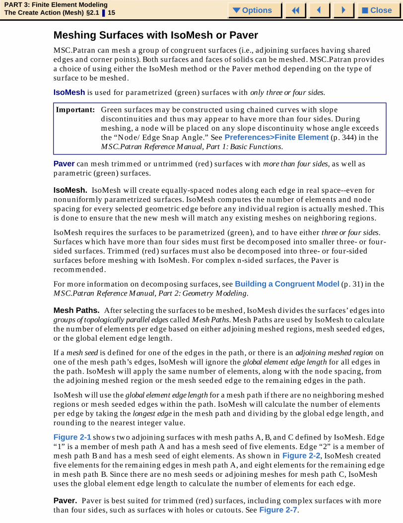
Meshing Surfaces with IsoMesh or PaverMSC.Patran can mesh a group of congruent surfaces (i.e., adjoining surfaces having shared edges and corner points). Both surfaces and faces of solids can be meshed. MSC.Patran provides a choice of using either the IsoMesh method or the Paver method depending on the type of surface to be meshed.
IsoMesh is used for parametrized (green) surfaces with only three or four sides.
Paver can mesh trimmed or untrimmed (red) surfaces with more than four sides, as well as parametric (green) surfaces.
IsoMesh. IsoMesh will create equally-spaced nodes along each edge in real space--even for nonuniformly parametrized surfaces. IsoMesh computes the number of elements and node spacing for every selected geometric edge before any individual region is actually meshed. This is done to ensure that the new mesh will match any existing meshes on neighboring regions.
IsoMesh requires the surfaces to be parametrized (green), and to have either three or four sides. Surfaces which have more than four sides must first be decomposed into smaller three- or four-sided surfaces. Trimmed (red) surfaces must also be decomposed into three- or four-sided surfaces before meshing with IsoMesh. For complex n-sided surfaces, the Paver is recommended.
For more information on decomposing surfaces, see Building a Congruent Model (p. 31) in the MSC.Patran Reference Manual, Part 2: Geometry Modeling.
Mesh Paths. After selecting the surfaces to be meshed, IsoMesh divides the surfaces’ edges into groups of topologically parallel edges called Mesh Paths. Mesh Paths are used by IsoMesh to calculate the number of elements per edge based on either adjoining meshed regions, mesh seeded edges, or the global element edge length.
If a mesh seed is defined for one of the edges in the path, or there is an adjoining meshed region on one of the mesh path’s edges, IsoMesh will ignore the global element edge length for all edges in the path. IsoMesh will apply the same number of elements, along with the node spacing, from the adjoining meshed region or the mesh seeded edge to the remaining edges in the path.
IsoMesh will use the global element edge length for a mesh path if there are no neighboring meshed regions or mesh seeded edges within the path. IsoMesh will calculate the number of elements per edge by taking the longest edge in the mesh path and dividing by the global edge length, and rounding to the nearest integer value.
Figure 2-1 shows two adjoining surfaces with mesh paths A, B, and C defined by IsoMesh. Edge “1” is a member of mesh path A and has a mesh seed of five elements. Edge “2” is a member of mesh path B and has a mesh seed of eight elements. As shown in Figure 2-2, IsoMesh created five elements for the remaining edges in mesh path A, and eight elements for the remaining edge in mesh path B. Since there are no mesh seeds or adjoining meshes for mesh path C, IsoMesh uses the global element edge length to calculate the number of elements for each edge.
Paver. Paver is best suited for trimmed (red) surfaces, including complex surfaces with more than four sides, such as surfaces with holes or cutouts. See Figure 2-7.
Important: Green surfaces may be constructed using chained curves with slope discontinuities and thus may appear to have more than four sides. During meshing, a node will be placed on any slope discontinuity whose angle exceeds the “Node/Edge Snap Angle.” See Preferences>Finite Element (p. 344) in the MSC.Patran Reference Manual, Part 1: Basic Functions.

CloseOptionsPART 3: Finite Element ModelingThe Create Action (Mesh) §2.1 16 Options
Paver is also good for surfaces requiring “steep” mesh transitions, such as going from four to 20 elements across a surface. Similar to IsoMesh, the paver calculates the node locations in real space, but it does not require the surfaces to be parametrized.
Important: For an all quadrilateral element mesh, the Paver requires the total number of elements around the perimeter of each surface to be an even number. It will automatically adjust the number of elements on a free edge to ensure this condition is met.

CloseOptionsPART 3: Finite Element ModelingThe Create Action (Mesh) §2.1 17 Options
Meshing SolidsMSC.Patran meshes solids with the IsoMesh or TetMesh.
IsoMesh can mesh any group of congruent triparametric (blue) solids (i.e., adjoining solids having shared edges and corner points). Triparametric solids with the topological shape of a brick or a wedge can be meshed with either hex or wedge elements. Any other form of triparametric solid can only be meshed with tet elements. Solids that have more than six faces must first be modified and decomposed before meshing.
TetMesh can be used to mesh all (blue or white) solids in MSC.Patran.
Mesh Paths. Since IsoMesh is used to mesh solids, similar to meshing surfaces, Mesh Paths are used to determine the number of elements per solid edge. For more detailed information on Mesh Paths, see Meshing Surfaces with IsoMesh or Paver (p. 15).
If there is a preexisting mesh adjoining one of the edges or a defined mesh seed on one of the edges in a mesh path, MSC.Patran will apply the same number of elements to the remaining edges in the path. If there are no adjoining meshes or mesh seeds defined within a path, the global element edge length will be used to determine the number of elements.
Figure 2-3 shows two adjoining congruent solids with mesh Paths A, B, C, and D defined. Edge “1” of path A has a mesh seed of five elements. Edge “2” of path B has a mesh seed of fourteen elements. And Edge “3” of path C has a nonuniform mesh seed of six elements. See Mesh Seeding (p. 19) for more information.
Figure 2-4 shows the solid mesh. Since Mesh Path A has a seed of five elements, all edges in the path are also meshed with five elements. The same applies for Mesh Paths B and C, where the seeded edge in each path determines the number of elements and node spacing. Since Mesh Path D did not have a mesh seed, or a preexisting adjoining mesh, the global element edge length was used to define the number of elements.
TetMesh. TetMesh will attempt to mesh any solid with very little input from the user as to what size of elements should be created. Generally, this is not what is needed for an actual engineering analysis. The following tips will assist the user both in terms of getting a good quality mesh suitable for the analysis phase and also tend to improve the success of TetMesh. If TetMesh fails to complete the mesh and the user has only specified a Global Length on the form, success might still be obtained by following some of the suggestions below.
Try to mesh the surfaces of a solid with the Paver using tria elements. If the Paver cannot mesh the solid faces, it is unlikely that TetMesh will be able to mesh the solid. By paving the solid faces first, much better control of the final mesh can be obtained. The mesh can be refined locally as needed. The surface meshing may also expose any problems with the geometry that make it difficult or impossible to mesh. Then these problems can be corrected before undertaking the time and expense to attempt to TetMesh the solid.
If higher order elements are required from a surface mesh of triangular elements, the triangular elements must also be of the corresponding order so that the mid edge nodes would be snapped properly.
Tria meshes on the solid faces can be left on the faces and stored in the database. This allows them to be used in the future as controls for the tet mesh in the solid at a later time.
After the tria mesh is created on the solid faces, it should be inspected for poor quality tria elements. These poor quality elements typically occur because Paver meshed a small feature in the geometry that was left over from the construction of the geometry, but is not important to

CloseOptionsPART 3: Finite Element ModelingThe Create Action (Mesh) §2.1 18 Options
the analysis. If these features are removed prior to meshing or if the tria mesh is cleaned up prior to tet meshing, better success rates and better tet meshes will usually follow. Look for high aspect ratios in the tria elements and look for tria elements with very small area.
The following paragraph applies only to the State Machine Algorithm.
Once the solid faces have a tria mesh, TetMesh will match the tet element faces to the existing tria elements. Just select the solid as input to TetMesh. This is not the same as selecting the tria shell as input. By selecting the solid, the resulting tet mesh will be associated with the solid and the element mid-edge nodes on the boundary will follow the curvature of the geometry. Note that the tria mesh on the solid faces do not need to be higher order elements in order for a higher order tet mesh to snap its mid-edge nodes to the geometry.

CloseOptionsPART 3: Finite Element ModelingThe Create Action (Mesh) §2.1 19 Options
Mesh Seeding
Mesh Transitions. A mesh transition occurs when the number of elements differs across two opposing edges of a surface or solid face. Mesh transitions are created either by mesh seeding the two opposing edges with a different number of elements, or by existing meshes on opposite sides of the surface or solid face, whose number of elements differ.
If IsoMesh is used for the transition mesh, MSC.Patran uses smoothing parameters to create the mesh. For most transition meshes, it is unnecessary to redefine the parameter values. See IsoMesh Parameters Subordinate Form (p. 43).
Seeding Surface Transitions. MSC.Patran can mesh a set of surfaces for any combination of mesh seeds. A mesh transition can occur in both directions of a surface.
Seeding Solid Transitions. Transition meshes for solids can only occur in two of three directions of the solids. That is, the transition can be defined on one side of a set of solids, and carried through the solids’ third direction. If a transition is required in all three directions, the user must break one of the solids into two, and perform the transition in two steps, one in each sub-solid. If a set of solids are seeded so that a transition will take place in all three directions, MSC.Patran will issue an error and not mesh the given set of solids.
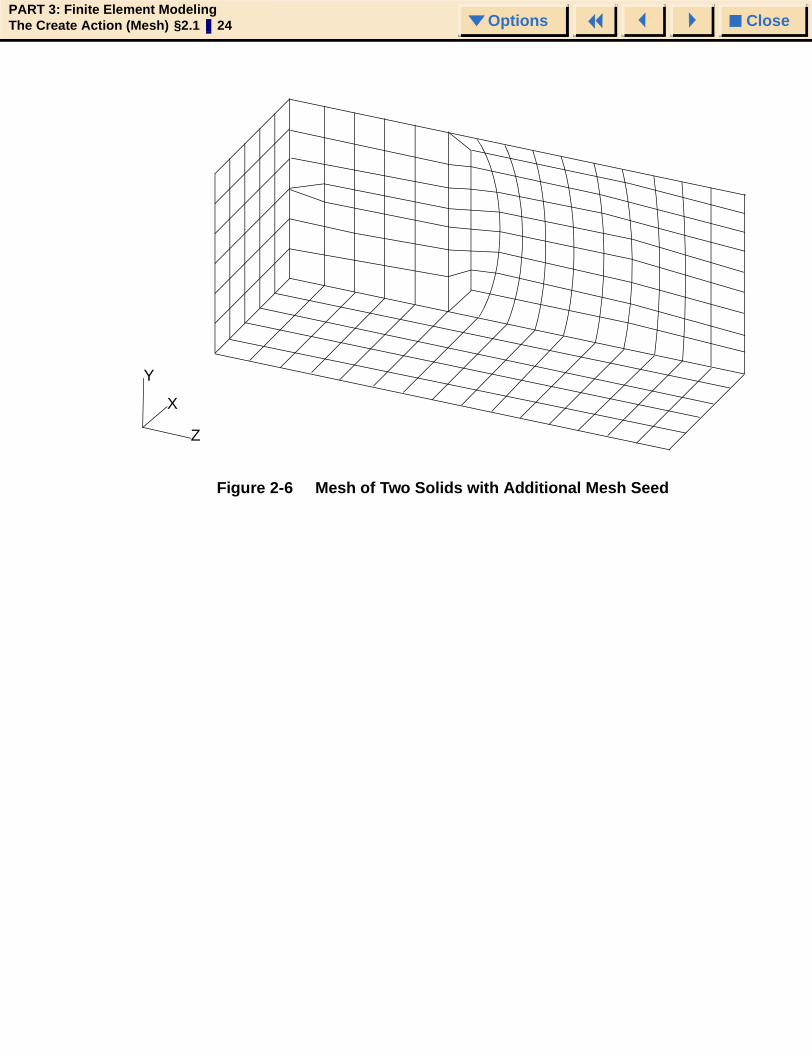
If more than one mesh seed is defined within a single mesh path (a mesh path is a group of topologically parallel edges for a given set of solids), it must belong to the same solid face. Otherwise, MSC.Patran will issue an error and not mesh the specified set of solids (see Figure 2-5 and Figure 2-6). If this occurs, additional mesh seeds will be required in the mesh path to further define the transition. For more information on mesh paths, see Mesh Solid (p. 42).
Avoiding Triangular Elements. MSC.Patran will try to avoid inserting triangle elements in a quadrilateral surface mesh, or wedge elements in a hexagonal solid mesh.
However, if the total number of elements around the perimeter of a surface, or a solid face is an odd number, the IsoMesh method will produce one triangular or one row of wedge element per surface or solid. Remember IsoMesh is the default meshing method for solids, as well as for curves.
If the total number of elements around the surface’s or solid’s perimeter is even, IsoMesh will mesh the surface or solid with Quad or Hex elements only. If the surface or solid is triangular or wedge shaped, and the mesh pattern chosen on the IsoMesh Parameters Subordinate Form (p. 43) form is the triangular pattern, triangle or wedge elements will be created regardless of the number of elements.
Figure 2-8 through Figure 2-13 show examples of avoiding triangular elements with IsoMesh.
When Quad elements are the desired element type, MSC.Patran’s Paver requires the number of elements around the perimeter of the surface to be even. If the number is odd, an error will be issued and Paver will ask the user if he wishes to use tri elements for this surface. If Quad elements are desired, the user must readjust the mesh seeds to an even number before meshing the surface again.

CloseOptionsPART 3: Finite Element ModelingThe Create Action (Mesh) §2.1 20 Options
Surface Mesh ControlUsers can specify surface mesh control on selected surfaces to be used when meshing using any of the auto meshers. This option allows users to create meshes with transition without having to do so one surface at a time. This option is particularly useful when used with the solid tet mesher to create mesh densities that are different on the edge and on the solid surface.

CloseOptionsPART 3: Finite Element ModelingThe Create Action (Mesh) §2.1 21 Options
Remeshing and ReseedingAn existing mesh or mesh seed does not need to be deleted before remeshing or reseeding. MSC.Patran will ask for permission to delete the existing mesh or mesh seed before creating a new one.
However, mesh seeds cannot be applied to edges with an existing mesh, unless the mesh seed will exactly match the number of elements and node spacing of the existing mesh. Users must first delete the existing mesh, before applying a new mesh seed to the edge.
Figure 2-1 IsoMesh Mesh Paths A, B, C
X
Y
Z
B
AA
B
A
C
C
Edge 2
Edge 1

CloseOptionsPART 3: Finite Element ModelingThe Create Action (Mesh) §2.1 22 Options
Figure 2-2 Meshed Surfaces Using IsoMesh
Figure 2-3 Mesh Seeding for Two Solids
X
Y
Z
A A A
C
C
B
B
X
Y
Z
C
D
A
DA
C
C
D
A
C
D
B
B
B
AB
D
A
D
A
Edge “2”
Edge “3”
Edge “1”

CloseOptionsPART 3: Finite Element ModelingThe Create Action (Mesh) §2.1 23 Options
Figure 2-4 Mesh of Two Solids With Seeding Defined
Figure 2-5 Incomplete Mesh Seed Definition for Two Solids
C
D
A
D
A
C
C
D
A
B
B
B
D
A
X
Y
Z
Mesh Seeds onTwo differentSolid Faces
CloseOptionsPART 3: Finite Element ModelingThe Create Action (Mesh) §2.1 24 Options
Figure 2-6 Mesh of Two Solids with Additional Mesh Seed
X
Y
Z

CloseOptionsPART 3: Finite Element ModelingThe Create Action (Mesh) §2.1 25 Options
Figure 2-7 Surface Mesh Produced by Paver
X
Y
Z

CloseOptionsPART 3: Finite Element ModelingThe Create Action (Mesh) §2.1 26 Options
Figure 2-8 Odd Number of Elements Around Surface Perimeter
Figure 2-9 Even Number of Elements Around Surface Perimeter
X
Y
Z
X
Y
Z

CloseOptionsPART 3: Finite Element ModelingThe Create Action (Mesh) §2.1 27 Options
Figure 2-10 Odd Mesh Seed
Figure 2-11 Even Mesh Seed
X
Y
Z
X
Y
Z

CloseOptionsPART 3: Finite Element ModelingThe Create Action (Mesh) §2.1 28 Options
Figure 2-12 Mesh Seeding Triangular Surfaces (1 Tria Produced)
Figure 2-13 Mesh Seeding Triangular Surfaces to Produce only Quad Elements
X
Y
Z
Mesh Seeded Elements is ODD.
X
Y
Z
IsoMesh will adjust # elements around perimeter to be even.

CloseOptionsPART 3: Finite Element ModelingThe Create Action (Mesh) §2.2 29 Options
2.2 Mesh Seed and Mesh Forms
Creating a Mesh Seed
❏ Uniform Mesh Seed
❏ One Way Bias Mesh Seed
❏ Two Way Bias Mesh Seed
❏ Curvature Based Mesh Seed
❏ Tabular Mesh Seed
❏ PCL Function Mesh Seed
Creating a Mesh
❏ IsoMesh Curve
❏ IsoMesh 2 Curves
❏ IsoMesh Surface
❏ Solid

CloseOptionsPART 3: Finite Element ModelingThe Create Action (Mesh) §2.2 30 Options
Creating a Mesh SeedThere are many types of mesh seeds: uniform, one way bias, two way bias, curvature based, and tabular.
Uniform Mesh Seed
Create mesh seed definition for a given curve, or an edge of a surface or solid, with a uniform element edge length specified either by a total number of elements or by a general element edge length. The mesh seed will be represented by small yellow circles and displayed only when the Finite Element form is set to creating a Mesh, or creating or deleting a Mesh Seed.
Define node spacing for mesh seed, by either pressing “Number of Elements” or “Element Length (L).” If “Number of Elements” is pressed, the user must then enter an integer value for the desired number of elements. If “Element Length” is pressed, then the user must enter an element edge length (MSC.Patran will calculate the resulting number of elements needed -rounded off to the nearest integer value.
If Auto Execute is selected, MSC.Patran will automatically create a mesh seed definition after each edge is selected. By default Auto Execute is OFF.
Specify list of curves by either cursor selecting existing curves or surface or solid edges, or specifying curve IDs or surface or solid edge IDs. (Example: Curve 10, Surface 12.1, Solid 22.5.2.)
MSC.Patran will plot all defined mesh seeds associated with the visible geometry.
Finite Elements
Action: Create
Object: Mesh Seed
Type: Uniform
Display Existing Seeds
Element Edge Length Data
Number of Elements
Element Length (L)
Number = 2
Auto Execute
Curve List
-Apply -
Type:
L
◆
◆◆
For more information see One Way Bias Mesh Seed (p. 31), Two Way Bias Mesh Seed (p. 32), Curvature Based Mesh Seed (p. 33), Tabular Mesh Seed (p. 34) or PCL Function Mesh Seed (p. 36).

CloseOptionsPART 3: Finite Element ModelingThe Create Action (Mesh) §2.2 31 Options
One Way Bias Mesh Seed
Create mesh seed definition for a given curve, or an edge of a surface or solid, with an increasing or decreasing element edge length, specified either by a total number of elements with a length ratio, or by actual edge lengths. The mesh seed will be represented by small yellow circles and is displayed only when the Finite Element form is set to creating a Mesh, or creating or deleting a Mesh Seed.
Define node spacing for mesh seed, by either pressing “Num Elems and L2⁄L1” or “L1 and L2”.
If “Num Elems and L2 ⁄L1” is pressed, the user must enter an integer value for the desired number of elements and an edge length ratio as indicated by the diagram. If “L1 and L2” is pressed, the user must enter edge lengths for the first and last elements.
MSC.Patran will calculate the nonuniform mesh seed node spacing through a geometric progression based on the given L2 ⁄L1 ratio. The positive edge direction for L1 and L2 as indicated by the arrow in the diagram is displayed in the current viewport.
If Auto Execute is selected, MSC.Patran will automatically create a mesh seed definition after each edge is selected. By default Auto Execute is OFF.
Specifies a list of edges by either cursor selecting existing curves or surface or solid edges, or specifying curve IDs or surface or solid edge IDs. (Example: Curve 10, Surface 12.1, Solid 22.5.2.)
MSC.Patran will plot all defined mesh seeds associated with the visible geometry.
Finite Elements
Action: Create
Object: Mesh Seed
Type: One Way Bias
Display Existing Seeds
Element Edge Length Data
Num Elems and L2/L1
L1 and L2
Number = 2
Auto Execute
Curve List
-Apply -
Type:
◆
◆◆
L2/L1 = 1.5
LL1 L2
CloseOptionsPART 3: Finite Element ModelingThe Create Action (Mesh) §2.2 32 Options
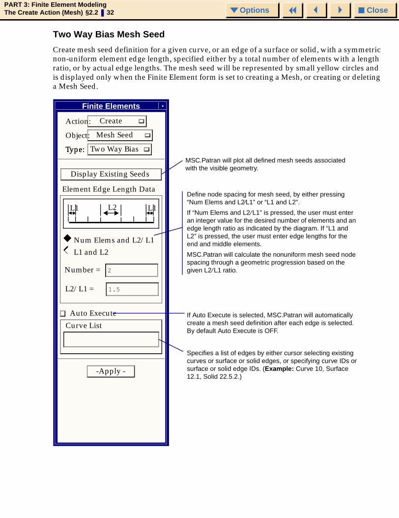
Two Way Bias Mesh Seed
Create mesh seed definition for a given curve, or an edge of a surface or solid, with a symmetric non-uniform element edge length, specified either by a total number of elements with a length ratio, or by actual edge lengths. The mesh seed will be represented by small yellow circles and is displayed only when the Finite Element form is set to creating a Mesh, or creating or deleting a Mesh Seed.
Define node spacing for mesh seed, by either pressing “Num Elems and L2⁄L1” or “L1 and L2”.
If “Num Elems and L2 ⁄L1” is pressed, the user must enter an integer value for the desired number of elements and an edge length ratio as indicated by the diagram. If “L1 and L2” is pressed, the user must enter edge lengths for the end and middle elements.
MSC.Patran will calculate the nonuniform mesh seed node spacing through a geometric progression based on the given L2 ⁄L1 ratio.
If Auto Execute is selected, MSC.Patran will automatically create a mesh seed definition after each edge is selected. By default Auto Execute is OFF.
Specifies a list of edges by either cursor selecting existing curves or surface or solid edges, or specifying curve IDs or surface or solid edge IDs. (Example: Curve 10, Surface 12.1, Solid 22.5.2.)
MSC.Patran will plot all defined mesh seeds associated with the visible geometry.
Finite Elements
Action: Create
Object: Mesh Seed
Type: Two Way Bias
Display Existing Seeds
Element Edge Length Data
Num Elems and L2/L1
L1 and L2
Number = 2
Auto Execute
Curve List
-Apply -
Type:
◆
◆◆
L2/L1 = 1.5
L2L1 L1
CloseOptionsPART 3: Finite Element ModelingThe Create Action (Mesh) §2.2 33 Options
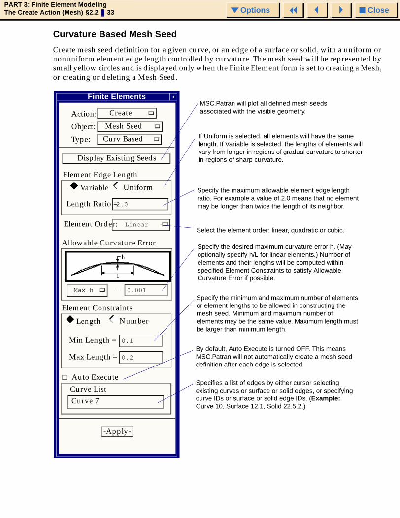
Curvature Based Mesh Seed
Create mesh seed definition for a given curve, or an edge of a surface or solid, with a uniform or nonuniform element edge length controlled by curvature. The mesh seed will be represented by small yellow circles and is displayed only when the Finite Element form is set to creating a Mesh, or creating or deleting a Mesh Seed.
MSC.Patran will plot all defined mesh seeds associated with the visible geometry.
If Uniform is selected, all elements will have the same length. If Variable is selected, the lengths of elements will vary from longer in regions of gradual curvature to shorter in regions of sharp curvature.
Specify the maximum allowable element edge length ratio. For example a value of 2.0 means that no element may be longer than twice the length of its neighbor.
By default, Auto Execute is turned OFF. This means MSC.Patran will not automatically create a mesh seed definition after each edge is selected.
Specify the minimum and maximum number of elements or element lengths to be allowed in constructing the mesh seed. Minimum and maximum number of elements may be the same value. Maximum length must be larger than minimum length.
Specifies a list of edges by either cursor selecting existing curves or surface or solid edges, or specifying curve IDs or surface or solid edge IDs. (Example: Curve 10, Surface 12.1, Solid 22.5.2.)
Action: Create
Object: Mesh Seed
Type: Curv Based
Display Existing Seeds
Element Edge Length
Variable Uniform
Allowable Curvature Error
0.001
Element Constraints
Length Number
Min Length = 0.1
Max Length = 0.2
Auto Execute
Curve List
◆ ◆◆
◆ ◆◆
Finite Elements
Curve 7
Length Ratio = 2.0
Element Order: Linear
Max h =
-Apply-
Select the element order: linear, quadratic or cubic.
Specify the desired maximum curvature error h. (May optionally specify h/L for linear elements.) Number of elements and their lengths will be computed within specified Element Constraints to satisfy Allowable Curvature Error if possible.

CloseOptionsPART 3: Finite Element ModelingThe Create Action (Mesh) §2.2 34 Options
Tabular Mesh Seed
Create mesh seed definition for a given curve, or an edge of a surface or solid, with an arbitrary distribution of seed locations defined by tabular values. The mesh seed will be represented by small yellow circles and is displayed only when the Finite Element form is set to creating a Mesh, or creating or deleting a Mesh Seed.
Finite Elements
Specify the coordinate type for the node locations. For example, if Arc length is selected, 0.5 will be located at the mid point of the curve. If Parametric is selected, 0.5 will be located at u=0.5 along the curve.
See next page for Nodes or Points option
Enter the desired node location values. Values can range between 0.0 and 1.0. The values 0.0 and 1.0 will be automatically added if they are omitted.
MSC.Patran will plot all defined mesh seeds associated with all visible geometry.
Blanks out all cells.
Specify a list of curves or edges of surfaces or solids to which the mesh seeds should be applied. (Example: Curve 10, Surface 1.4, Solid 1.8.5.)
By default Auto Execute is turned OFF.
Sorts all the values entered in ascending order.
Reverses the node locations by replacing v with 1.0 - v.
Action: Create
Object: Mesh Seed
Type: Tabular
Display Existing Seeds
Input Data
Clear Sort Reverse
Auto ExecuteCurve List
-Apply-
3
54
21
6
Arc Length Value
Coordinate Type
Arc LengthParametricNodes or Points
◆
◆◆
Seed Location Data
◆◆

CloseOptionsPART 3: Finite Element ModelingThe Create Action (Mesh) §2.2 35 Options
Tolerance to be used when creating a seed with Nodes/Points entered in Nodes or Points List.
List of Nodes and or points to be used to create a seed. Only those within the tolerance specified to the curve selected will be used for creating the seed.
Enter a list of nodes, points, or pick locations on screen.
Curve ID on which the seed should be created.
Finite Elements
Action: Create
Object: Mesh Seed
Type: Tabular
Display Existing Seeds
Coordinate Type
Arc LengthParametricNodes or Points
Tolerance 0.005
Nodes or Points List
Auto Execute
Curve Id
-Apply-
◆
◆◆
◆◆

CloseOptionsPART 3: Finite Element ModelingThe Create Action (Mesh) §2.2 36 Options
PCL Function Mesh Seed
Create mesh seed definition for a given curve, or an edge of a surface or solid, with a distribution of seed locations defined by a PCL function. The mesh seed will be represented by small yellow circles and is displayed only when the Finite Element form is set to creating a Mesh, or creating or deleting a Mesh Seed.
Selecting one of the predefined functions will enter its call into the “PCL for jth Node” data box where it can be edited if desired. These functions exist in the PCL library supplied with MSC.Patran. Sample code is presented on the next page for use as a model in writing your own function.
Enter an inline PCL function or a call to an existing compiled function. A trivial example of an inline function is one that computes a unifor seed:
(j-1)/N-1)
MSC.Patran will plot all defined mesh seeds associated with all visible geometry.
Specify a list of curves or edges of surfaces or solids to which the mesh seeds should be applied.
(Example: Curve 10, Surface 1.4, Solid 22.5.3)
By default Auto Execute is turned OFF.
Enter the number of nodes (seeds) to be created.
Finite Elements
Action: Create
Object: Mesh Seed
Type: PCL Function
Display Existing Seeds
Seed Definition
Number of Nodes (N)
10
Predefined Functions
BetaClusterRoberts
PCL for jth Node
Auto Execute
Curve List
-Apply-

CloseOptionsPART 3: Finite Element ModelingThe Create Action (Mesh) §2.2 37 Options
The following is the PCL code for the predefined function called beta. It may be used as a model for writing your own PCL function.
FUNCTION beta(j, N, b)GLOBAL INTEGERj, NREALb, w, t, rval
x = (N - j) / (N - 1)t = ( ( b + 1.0 ) / ( b - 1.0 ) ) **wrval = ( (b + 1.0) - (b - 1.0) *t ) / (t + 1.0)RETURN rvalEND FUNCTION
Note: j and N MUST be the names for the first two arguments.
N is the number of nodes to be created, and j is the index of the node being created, where ( 1 <= j <= N ).
An individual user function can be accessed at run time by entering the command:
!!INPUT <my_pcl_function_file_name>
A library of precompiled PCL functions can be accessed by:
!!LIBRARY <my_plb_library_name>
For convenience these commandes can be entered into your p3epilog.pcl file so that the functions are available whenever you run MSC.Patran.
CloseOptionsPART 3: Finite Element ModelingThe Create Action (Mesh) §2.3 38 Options
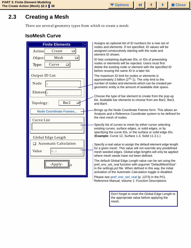
2.3 Creating a MeshThere are several geometry types from which to create a mesh:
IsoMesh CurveAssigns an optional list of ID numbers for a new set of nodes and elements. If not specified, ID values will be assigned consecutively starting with the node and element ID shown.
ID lists containing duplicate IDs, or IDs of preexisting nodes or elements will be rejected. Users must first delete the existing node or element with the specified ID before reusing the same ID in a later list.
The maximum ID limit for nodes or elements is approximately 2 billion (231-1). The only limit to the number of nodes and elements which can be created per geometric entity is the amount of available disk space.
Specify a real value to assign the default element edge length for a given mesh. This value will not override any predefined mesh seeded edges. Global edge lengths will only be applied where mesh seeds have not been defined.
The default Global Edge Length value can be set using the pref_env_set_real function with argumet “DefaultMeshSize” in the settings.pcl file. When defined in this way, the initial activation of the Automatic Calculation toggle is disabled.
Please see pref_env_set_real (p. 1373) in the PCL Reference Manual, Volume 1: Function Descriptions
Choose the type of bar element to create from the pop-up list. Available bar elements to choose from are Bar2, Bar3, and Bar4.
Specify list of curves to mesh by either cursor selecting existing curves, surface edges, or solid edges, or by specifying the curve IDs, or the surface or solid edge IDs. (Example: Curve 12, Surface 1.3, Solid 11.3.1.)
Brings up the Node Coordinate Frames form. This allows an Analysis and a Reference Coordinate system to be defined for the next mesh of nodes.
Don’t forget to reset the Global Edge Length to the appropriate value before applying the mesh.
Finite Elements
Action: Create
Object: Mesh
Type: Type: Curve
Output ID List
Node 1
Element 1
Global Edge Length
0.1
Node Coordinate Frames...
Curve List-Apply-
Curve List
Topology: Bar2
Value
Automatic Calculation

CloseOptionsPART 3: Finite Element ModelingThe Create Action (Mesh) §2.3 39 Options
IsoMesh 2 Curves
Finite Elements
Action: Create
Object: Mesh
Type: 2 Curves
Output ID List
Node 1
Element 1
Elem Shape Quad
Mesher IsoMesh
Topology Quad4
Auto Execute
Curve 1 List
Curve 2 List
Control Element Number
Global Edge Length
Automatic Calculation
Value 0.1
-Apply-
Tria6
IsoMesh Parameters...
Node Coordinate Frames...
Assigns an optional list of ID numbers for a new set of nodes and elements. If not specified, ID values will be assigned consecutively starting with the node and element ID shown.
ID lists containing duplicate IDs, or IDs of preexisting nodes or elements will be rejected. Users must first delete the existing node or element with the specified ID before reusing the same ID in a later list.
The maximum ID limit for nodes or elements is approximately 2 billion (231-1). The only limit to the number of nodes and elements which can be created per geometric entity is the amount of available disk space.
The default Global Edge Length value can be set using the pref_env_set_real function with argument “DefaultMeshSize” in the settings.pcl file. When defined in this way, the initial activation of the Automatic Calculation toggle is disabled.
Please see pref_env_set_real (p. 1373) in the PCL Reference Manual, Volume 1: Function Descriptions
Choose the type of Quad or Tria element to create from the given list. Available Quad and Tria elements to choose from are Quad4, Quad5, Quad8, Quad9, Quad12, Quad16, Tria3, Tria4, Tria6, Tria7, Tria9, Tria13.
Specify the two curve lists. Isomesh with selected element type will be created on a ruled surface connecting the two input curve lists.
Specify number of elements on edges or a real value to assign the default element edge length for a given mesh.
Both options will not override any predefined mesh seeded edges. Global edge lengths and element number will only be applied where mesh seeds have not been defined.

CloseOptionsPART 3: Finite Element ModelingThe Create Action (Mesh) §2.3 40 Options
IsoMesh Surface
Assigns an optional list of ID numbers for a new set of nodes and elements. If not specified, ID values will be assigned consecutively starting with the node and element ID shown.
ID lists containing duplicate IDs, or IDs of preexisting nodes or elements will be rejected. Users must first delete the existing node or element with the specified ID before reusing the same ID in a later list.
The maximum ID limit for nodes or elements is approximately 2 billion (231-1). The only limit to the number of nodes and elements which can be created per geometric entity is the amount of available disk space.
Specify a real value to assign the default element edge length for a given mesh. This value will not override any predefined mesh seeded edges. Global edge lengths will only be applied where mesh seeds have not been defined or where there are no existing adjacent meshed regions.
The default Global Edge Length value can be set using the pref_env_set_real function with argument “DefaultMeshSize” in the settings.pcl file. When defined in this way, the initial activation of the Automatic Calculation toggle is disabled.
Please see pref_env_set_real (p. 1373) in the PCL Reference Manual, Volume 1: Function Descriptions
Choose the type of Quad or Tria element to create from the given list. Available Quad and Tria elements to choose from are Quad4, Quad5, Quad8, Quad9, Quad12, Quad16, Tria3, Tria4, Tria6, Tria7, Tria9, Tria13.
Brings up the IsoMesh Parameters form which is used for transition meshes. This is an optional function that affects MSC.Patran’s IsoMesh smoothing algorithm For most transition meshes, it is not required to reset the default parameter values.
Specifies a list of surfaces to mesh by either cursor selecting existing surfaces, solid faces, or SGM trimmed faces, or entering the IDs of the surfaces, solid faces, and ⁄or SGM trimmed faces. (Example: Surface 23, Solid 11.3.)
Choose either the IsoMesh method or the Paver method of meshing. If Paver is selected the IsoMesh Parameters changes to Paver Parameters...
Brings up the Node Coordinate Frames form. This allows an Analysis and a Reference Coordinate system to be defined for the next mesh of nodes.
Don’t forget to reset the Global Edge Length to the appropriate value before applying the mesh.
Finite Elements
Action: Create
Object: Mesh
Type: Type: Surface
Output ID List
Node 1
Element
IsoMesh Parameters...
Node Coordinate Frames...
Surface List
-Apply-
1
Elem Shape Quad
Mesher IsoMesh
Topology Quad4
Global Edge Length
Automatic Calculation
Value 0.1

CloseOptionsPART 3: Finite Element ModelingThe Create Action (Mesh) §2.3 41 Options
Paver Parameters
Paver Parameters...
Create P-Element Mesh
Global Space Only
Allow Tris in Quad Mesh
Curvature Check
Allowable Curvature Error
0.250.
Max h/L = 0.1
Use Desired Edge Lengths
Min. Edge I/L : 0.0
Max. Edge Length : 0.0
DefaultsOk
Causes the mesher to relax its criteria for element quality in an attempt to create a coarser mesh.
Causes the mesher to adjust the mesh density to control the deviation between the geometry and the straight element edges. This will usually result in a better mesh and a better chance for success when meshing complicated geometry. Currently, this only works on edges only.
If Curvature Check is set, enter the desired maximum deviation between the element edges and geometry as the ratio of the deviation to element edge length. Deviation is measured at the center of the element edge. The value may be entered either by using the slider bar or by typing a value into the data box.
The Paver has more freedom to adjust the mesh size in the geometry interior. If this toggle is not set, then the meshers will try to make elements in the interior sized between the shortest and longest edge on the boundary, or the global length from the main meshing form, whichever is more extreme. This is how the paver worked in previous MSC.Patran releases. If this toggle is set and reasonable values for minimum and maximum element edge lengths are given, then the meshers will attempt to make elements in the interior of the meshing region with element edge lengths between the user defined values. This gives the user more control over the mesh in the interior of the geometry.
The Ok button must be clicked with the mouse in order to update the new values the user enters on this form and make them available to the meshers. If the button is not clicked, the new values will not be passed on to the meshers.
Used to restore all of the default settings to this form.
Mesh the surface in global space only, if the toggle is set.
Allows one tri element on a loop if the sum of all the element edges on the loop is an odd number.

CloseOptionsPART 3: Finite Element ModelingThe Create Action (Mesh) §2.3 42 Options
Solid
IsoMesh
Choose the type of Hex, Wedge or Tet element to create from the given list. Available solid elements to choose from are Hex8, Hex9, Hex20, Hex21, Hex26, Hex27, Hex32, Hex64, Wedge6, Wedge7, Wedge15, Wedge16, Wedge20,Wedge21, Wedge24, Wedge52, Tet4, Tet5, Tet10, Tet11, Tet14, Tet15, Tet16, Tet40.
Specifies a list of solids to mesh by either cursor selecting existing solids, or entering the IDs of the solids. (Example: Solid 23.)
Brings up the Node Coordinate Frames form which allows an Analysis and a Reference Coordinate system to be defined for the next mesh of nodes.
Assigns an optional list of ID numbers for a new set of nodes and elements. If not specified, ID values will be assigned consecutively starting with the node and element ID shown.
ID lists containing duplicate IDs, or IDs of preexisting nodes or elements will be rejected. Users must first delete the existing node or element with the specified ID before reusing the same ID in a later list.
The maximum ID limit for nodes or elements is approximately 2 billion (231- 1). The only limit to the number of nodes and elements that can be created per geometric entity is the amount of available disk space.
Specify a real value to assign the default element edge length for a given mesh. This value will not override any predefined mesh seeded edges. Global edge lengths will only be applied where mesh seeds have not been defined or where there are no existing adjacent meshed regions.
Finite Elements
Action: Create
Object: Mesh
Type: Type: Solid
IsoMesh Parameters...
Solid List
-Apply-
Brings up the IsoMesh Parameters form which is used for transition meshes. This is an optional function that affects MSC.Patran’s IsoMesh smoothing algorithm. For most transition meshes, it is not required to reset the default parameter values. If TetMesh is selected the IsoMesh Parameters changes to TetMesh Parameters...
Node Coordinate Frames...
Don’t forget to reset the Global Edge Length to the appropriate value before applying the mesh.
Elem Shape Tet
Mesher IsoMesh
Topology Tet4
Output ID List
Node 1
Element 1
Global Edge Length
Automatic Calculation
Value 0.1

CloseOptionsPART 3: Finite Element ModelingThe Create Action (Mesh) §2.3 43 Options
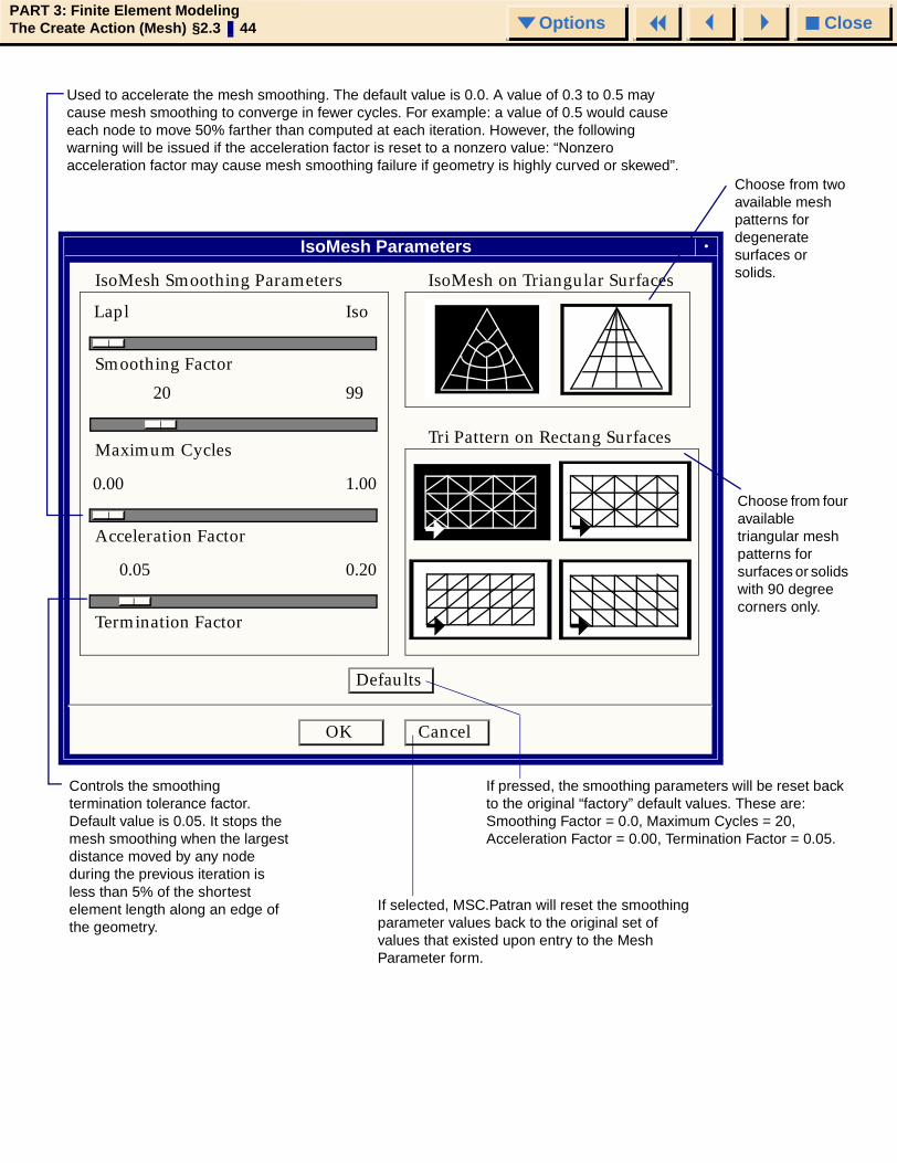
IsoMesh Parameters Subordinate Form. This form appears when the IsoMesh Parameters button is selected on the Finite Elements form.
Smoothing parameters affect only transition meshes. A transition occurs when two opposing edges of a surface differ in the number of elements or mesh ratio. The values may be changed by pressing the left mouse button and moving the slide bar to the appropriate value.
The smoothing algorithm used by MSC.Patran is the iterative Laplacian-Isoparametric scheme developed by L.R. Herrmann.
trans isopar
IsoMesh Parameters
Smoothing Factor
Lapl Iso
Maximum Cycles
Acceleration Factor
0.00 1.00
Termination Factor
0.05 0.20
IsoMesh Smoothing Parameters IsoMesh on Triangular Surfaces
tri1 tri2
Tri Pattern on Rectang Surfaces
Defaults
OK Cancel
Used to determine a weighted combination of Laplacian and Isoparametric smoothing methods. Valid range is from 0.0 to 1.0, where 0.0 is pure Laplacian smoothing and 1.0 is pure Isoparametric smoothing. Intermediate values mean a combination of the two methods will be used. The default value is 0.0. Laplacian smoothing is best for most transition cases, except where the surface has significant inplane curvature in that case, Isoparametric smoothing is best.
Maximum number of iterations allowed for mesh smoothing. Default value is 20. Smoothing may be turned off by setting the Maximum Cycles to zero.
20 99
CloseOptionsPART 3: Finite Element ModelingThe Create Action (Mesh) §2.3 44 Options
Controls the smoothing termination tolerance factor. Default value is 0.05. It stops the mesh smoothing when the largest distance moved by any node during the previous iteration is less than 5% of the shortest element length along an edge of the geometry.
If pressed, the smoothing parameters will be reset back to the original “factory” default values. These are: Smoothing Factor = 0.0, Maximum Cycles = 20, Acceleration Factor = 0.00, Termination Factor = 0.05.
Choose from four available triangular mesh patterns for surfaces or solids with 90 degree corners only.
If selected, MSC.Patran will reset the smoothing parameter values back to the original set of values that existed upon entry to the Mesh Parameter form.
trans isopar
IsoMesh Parameters
Smoothing Factor
Lapl Iso
Maximum Cycles
Acceleration Factor
0.00 1.00
Termination Factor
0.05 0.20
IsoMesh Smoothing Parameters IsoMesh on Triangular Surfaces
tri1 tri2
Tri Pattern on Rectang Surfaces
Defaults
OK Cancel
20 99
Used to accelerate the mesh smoothing. The default value is 0.0. A value of 0.3 to 0.5 may cause mesh smoothing to converge in fewer cycles. For example: a value of 0.5 would cause each node to move 50% farther than computed at each iteration. However, the following warning will be issued if the acceleration factor is reset to a nonzero value: “Nonzero acceleration factor may cause mesh smoothing failure if geometry is highly curved or skewed”.
Choose from two available mesh patterns for degenerate surfaces or solids.

CloseOptionsPART 3: Finite Element ModelingThe Create Action (Mesh) §2.3 45 Options
TetMesh
Using the Create/Mesh/Solid form with the TetMesh button pressed creates a set of four node, 10 node or 16 node tetrahedron elements for a specified set of solids. The solids can be composed of any number of sides or faces.
Finite Elements
Action: Create
Object: Mesh
Type: Solid
Output ID List
Node 1
Element 1
Elem Shape Tet
Mesher TetMesh
Topology Tet4
Input List
Global Edge Length
Automatic Calculation
Value 0.1
Match Parasolid Faces
-Apply-
Node Coordinate Frames...
TetMesh Parameters...
Specify the existing solids to mesh, either by cursor selecting them or by entering the IDs from the keyboard. (Example: Solid 1:10) The select filter may be used to select the triangular elements that form a closed volume.
Select the type of tetrahedron element that you want to mesh with. The available choices are: Tet4, Tet10, and Tet16.
Defines the default element edge length for the mesh. This value will not override any existing mesh seeded edges. MSC.Patran will only apply the Global Edge Length to those areas of the mesh where mesh seeds have not been defined or where there are no existing nodes or adjacent meshes. (If the value is small relative to the size of the solid, a very large number of Tet elements may be generated.) The default is 0.1.
Shows the IDs that will be assigned consecutively starting with the node and element ID shown.
If you specify a list of IDs that contain duplicate IDs or IDs that are assigned to existing nodes or elements, the list will be rejected. You must first delete the existing node or element with the specified ID before reusing the ID in the Node or Element ID List.
Assembly Meshing of multiple parasolid solids. Turning this toggle ON maintains a congruent mesh between multiple parasolid solids. This is not supported for Patran solids. If solids are within parasolid tolerance (1.0E-6), then solids which do not match topologically will be forced to match in the resultant mesh. If solids are outside parasolid tolerance but within the tolerance specified on the Tetmesh Parameters form, then only solids which have matching topology will be meshed congruently.
Create Duplicate Nodes
Allows the creation of a duplicate set of nodes for each entity which is matching between solids in Assembly Meshing. Equivalencing using the above tolerance value will remove these duplicate nodes. This toggle also applies to assembly meshing, for example using Match Parasolid Faces, where a duplicate set of nodes will be created on entities that are found to be shared between solids. The only time duplicate nodes will be created while the toggle is off is where an existing mesh is transferred to a solid

CloseOptionsPART 3: Finite Element ModelingThe Create Action (Mesh) §2.3 46 Options
Value 0.1
Match Parasolid Faces
-Apply-
The duplicate nodes toggle will create an extra set of nodes on geometry that is shared between more than one solid, for example on a face that is shared between two solids.
This toggle also applies to assembly meshing, for example, using Match Parasolid Faces, where a duplicate set of nodes will be created on entities that are found to be shared between solids. The only situation in assembly meshing where duplicate nodes will be created with the toggle off is where an existing mesh is being transferred from a neighboring solid.
Create Duplicate Nodes
Neighbor Solid List
Preview Interface MeshWith the Neighbor Solid List you can Match the mesh of the neighboring solids.
☞ More Help:• Creating a Boundary Representation (B-
rep) Solid (p. 338) in the MSC.Patran Reference Manual, Part 2: Geometry Modeling
• Solids (p. 24) in the MSC.Patran Reference Manual, Part 2: Geometry Modeling
• Verify - Element (Normals) (p. 142)
With Preview Interface Mesh ON, you can view the mesh before applying the mesh to your model.

CloseOptionsPART 3: Finite Element ModelingThe Create Action (Mesh) §2.3 47 Options
TetMesh Parameters
The TetMesh Parameters sub-form allows you to change meshing parameters for P-Element meshing and Curvature based refinement.
TetMesh Parameters...
Create P-Element Mesh
Internal Coarsening
Curvature Check
Refinement Options
Maximum h/L = 0.1
Minimum Edge Length =
Global Edge Length* 0.2
DefaultsOK
0.250.
When creating a mesh with mid-side nodes (such as with Tet10 elements) in a solid with curved faces, it is possible to create elements that have a negative Jacobian ratio which is unacceptable to finite element solvers. To prevent an error from occurring during downstream solution pre-processing, the edges for these negative Jacobian elements are automatically straightened resulting in a positive Jacobian element. Although the solver will accept this element's Jacobian, the element edge is a straight line and no longer conforms to the original curved geometry. If this toggle is enabled before the meshing process, the element edges causing a negative Jacobian will conform to the geometry, but will be invalid elements for most solvers. To preserve edge conformance to the geometry, the "Modify-Mesh-Solid" functionality can then be utilized to locally remesh the elements near the elements containing a negative Jacobian.
To create a finer mesh in regions of high curvature, the "Curvature Check" toggle should be turned ON. There are two options to control the refinement parameters. Reducing the "Maximum h/L" creates more elements in regions of high curvature to lower the distance between the geometry and the element edge. The "Minimum l/L" option controls the lower limit of how small the element size can be reduced in curved regions. The ratio l/L is the size of the minimum refined element edge to the "Global Edge Length" specified on the "Create-Mesh-Solid" form.
The tetrahedral mesh generator has an option to allow for transition of the mesh from a very small size to the user given Global Edge Length. This option can be invoked by turning the Internal Coarsening toggle ON. This option is supported only when a solid is selected for meshing. The internal grading is governed by a growth factor, which is same as that used for grading the surface meshes in areas of high curvature (1:1.5). The elements are gradually stretched using the grade factor until it reaches the user given Global Edge Length. After reaching the Global Edge Length the mesh size remains constant.

CloseOptionsPART 3: Finite Element ModelingThe Create Action (Mesh) §2.3 48 Options
Node Coordinate Frames
Specifies local coordinate frame ID for analysis results. The default coordinate frame ID is defined under the Global Preferences menu, usually the global rectangular frame ID of zero.
Specifies an existing local coordinate frame ID to associate with the set of meshed nodes. The nodes’ locations can later be shown or modified within the specified reference frame. See The Show Action (Ch. 12). The default coordinate frame ID is defined under the Global Preferences menu, usually the global rectangular frame ID of zero.
Node Coordinate Frames
Analysis Coordinate Frame
Coord 0
Refer. Coordinate Frame
Coord 0
OK
CloseOptionsPART 3: Finite Element ModelingThe Create Action (Mesh) §2.4 49 Options
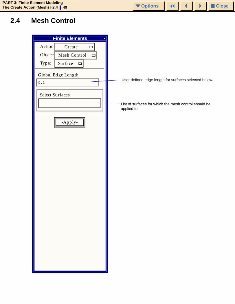
2.4 Mesh Control
Finite Elements
Action: Create
Object: Mesh Control
Type: Surface
Global Edge Length
0.1
Select Surfaces
-Apply-
User defined edge length for surfaces selected below.
List of surfaces for which the mesh control should be applied to.

CloseOptionsPART 3: Finite Element ModelingThe Create Action (Mesh) §2.4 50 Options
Auto Hard Points FormUsing the Create/Mesh Control/Auto Hard Points form creates hard points on a specified set of surfaces automatically. This program creates hard points at two kinds of points on surface boundaries: T Points - A T point is defined as an interior point of a surface edge which is close to a vertex or an existing hard point on an edge in another surface within the t-point tolerance. The t-point tolerance is equal to one twentieth of the target element edge length. Placing a hard point at a T-point will help meshers create a congruent mesh on a noncongruent model. There is a noncongruent model in Figure 2-14. The auto hard point creation program creates a T-point at the T-junction of three surfaces and marks it by a small triangle. The new hard point forces the mesher to place a node at the T-junction when meshing surface 1 and the mesh created is a congruent mesh (Figure 2-15). Figure 2-16 shows the mesh without hard point creation.
Figure 2-14 T-Point Creation
Figure 2-15 Mesh with Hard Point Creation Figure 2-16 Mesh Without Hard Point Creation

CloseOptionsPART 3: Finite Element ModelingThe Create Action (Mesh) §2.4 51 Options
Neck Points. A neck point is defined as an end point of a short cross section on a surface. A cross section on a surface is short if its length is less than the neck-point tolerance.The neck-point tolerance is equal to 1.5 times the target element edge length. Placing a hard point at a neck point will help meshers create better meshes on narrow surfaces. Neck points can be created recursively by neck-point propagation. In Figure 2-17, the two neck-points on the boundary of surface 1 were created first and the remain four neck points were created by neck point propagation from one small surface to another until the path reached the outer boundary of the model. The new hard points will help mesher line up the boundary nodes and create a good mesh on the narrow surfaces (Figure 2-18). Figure 2-19 shows the mesh without hard point creation.
Figure 2-17 Neck Point Propagation
Figure 2-18 Mesh with Hard Point Creation Figure 2-19 Mesh Without Hard Point Creation

CloseOptionsPART 3: Finite Element ModelingThe Create Action (Mesh) §2.4 52 Options
Figure 2-20
Finite Elements
Action: Create
Object: Mesh Control
Type: Auto Hard Points
Target Element Edge Length
0.1
Surface List
-Apply-
Surface 1:8
Specify the target element edge length which you will use as a global edge length when you mesh the model. The target element edge length is used to compute the t-point tolerance and neck-point tolerance.
Specify a set of surfaces on which to create hard points, either by cursor selecting them or by entering the IDs from the keyboard. (Example: Surface 1:10).
CloseOptionsPART 3: Finite Element ModelingThe Create Action... § 53 Options
MSC.Patran Reference Manual, Part 3: Finite Element Modeling
CHAPTER
3 The Create Action (FEM Entities)
■ Introduction
■ Creating Nodes
■ Creating Elements
■ Creating MPCs
■ Creating Superelements
■ Creating DOF List
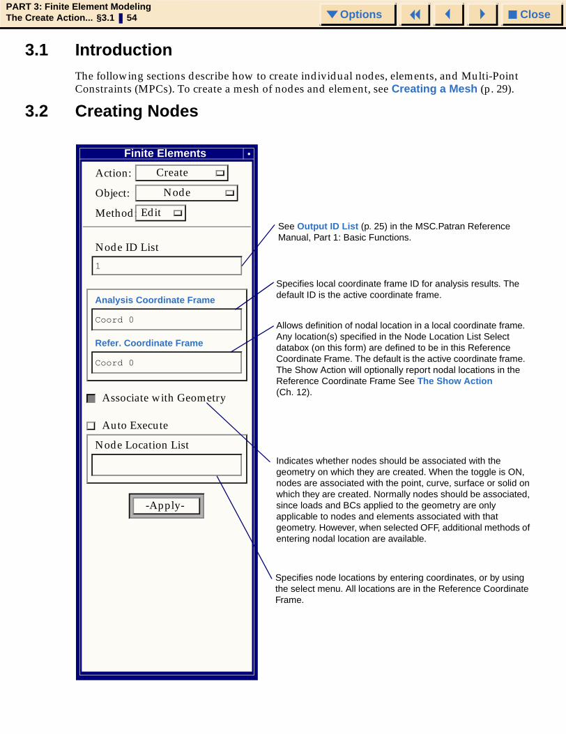
CloseOptionsPART 3: Finite Element ModelingThe Create Action... §3.1 54 Options
3.1 IntroductionThe following sections describe how to create individual nodes, elements, and Multi-Point Constraints (MPCs). To create a mesh of nodes and element, see Creating a Mesh (p. 29).
3.2 Creating Nodes
See Output ID List (p. 25) in the MSC.Patran Reference Manual, Part 1: Basic Functions.
Specifies local coordinate frame ID for analysis results. The default ID is the active coordinate frame.
Allows definition of nodal location in a local coordinate frame. Any location(s) specified in the Node Location List Select databox (on this form) are defined to be in this Reference Coordinate Frame. The default is the active coordinate frame. The Show Action will optionally report nodal locations in the Reference Coordinate Frame See The Show Action (Ch. 12).
Indicates whether nodes should be associated with the geometry on which they are created. When the toggle is ON, nodes are associated with the point, curve, surface or solid on which they are created. Normally nodes should be associated, since loads and BCs applied to the geometry are only applicable to nodes and elements associated with that geometry. However, when selected OFF, additional methods of entering nodal location are available.
Specifies node locations by entering coordinates, or by using the select menu. All locations are in the Reference Coordinate Frame.
Finite Elements
Action: Create
Object: Node
Method: Edit
Node ID List
1
Analysis Coordinate Frame
Coord 0
Refer. Coordinate Frame
Coord 0
Associate with Geometry
Auto Execute
Node Location List
-Apply-

CloseOptionsPART 3: Finite Element ModelingThe Create Action... §3.3 55 Options
3.3 Creating Elements
Select the shape of the element(s) to be created.
Choose an element topology (nodal connectivity). See The MSC.Patran Element Library (Ch. 15), for an illustrated list of MSC.Patran’s available topology.
When selected ON, duplicate mid-edge nodes will not be created along common boundaries of elements with similar topology. Instead, existing mid-edge nodes from adjacent elements will be used when appropriate. If selected OFF, new mid-edge nodes will always be created.
Specifies lists of element corner nodes. One select databox is displayed for each element corner node. Only the elements corner nodes need to be specified. Element midnodes will be automatically generated.
Multiple elements can be created by specifying multiple corner nodes in each select databox. For example, when creating Bar elements, if the list for corner node 1 contains nodes 10 and 11, and the list for corner node 2 contains nodes 13 and 14, two elements will be created: one between nodes 10 and 13, and one between nodes11 and 14.
If the number of nodes specified in each node list are not equal, the last specified node ID in each short list will be used to extend that list to the necessary length.
See Output ID List (p. 25) in the MSC.Patran Reference Manual, Part 1: Basic Functions.
Finite Elements
Action: Create
Object: Element
Method: Edit
Element ID List
1
Shape: Quad
Topology: Quad4
Pattern: Standard
Use existing midnodes
Auto Execute
Node 1 =
Node 2 =
Node 3 =
Node 4 =
-Apply-

CloseOptionsPART 3: Finite Element ModelingThe Create Action... §3.4 56 Options
3.4 Creating MPCs
Overview. An MPC (multi-point constraint) is a constraint that defines the response of one or more nodal degrees-of-freedom (called dependent degrees-of-freedom) to be a function of the response of one or more nodal degrees-of-freedom (called independent degrees-of-freedom). The general form of the MPC, which most of the major structural analysis codes support (referred to as the explicit MPC type in MSC.Patran) is as follows:
U0 = C1U1 + C2U2 + C3U3 + ... + CnUn + C0 Eq. 3-1
Where U0 is the dependent degree-of-freedom, Ui the independent degrees-of-freedom, and Ci the constants. The term to the left of the equal sign is called the dependent term and the terms to the right of the equal sign are called the independent terms. C0 is a special independent term called the constant term.
An example of an explicit MPC is:
UX(Node 4) = 0.5*UX(Node 5) - 0.5*UY(Node 10) + 1.0 Eq. 3-2
which specifies that the x displacement of node 4 is equal to half the x displacement of node 5 minus half they displacement of node 10 plus 1.0. There are four terms in this example, one dependent term, two independent terms, and a constant term.
MPC Types. MPCs can be used to model certain physical phenomena that cannot be easily modeled using finite elements, such as rigid links, joints (revolutes, universal, etc.), and sliders, to name a few. MPCs can also be used to allow load transfer between incompatible meshes. However, it is not always easy to determine the explicit MPC equation that correctly represents the phenomena you are trying to model.
To help with this problem, many analysis codes provide special types of MPCs (sometimes called “implicit” MPCs) which simulate a specific phenomena with minimum user input. For example, most analysis codes support an implicit MPC type which models a rigid link, in which an independent node is rigidly tied to one or more dependent nodes. All the user is required to input are the node IDs. The analysis code internally generates the “explicit” MPCs necessary to cause the nodes to act as if they are rigidly attached.
In addition to the implicit MPC types supported by the analysis code, there are implicit MPC types supported by the analysis code translator. These are converted into “explicit” form during the translation process. This allows MSC.Patran to support more MPC types than the analysis code supports itself.
MSC.Patran supports the creation of all MPC types through the use of a single form, called Create MPC Form (for all MPC Types Except Cyclic Symmetry and Sliding Surface) (p. 60), with two exceptions: the Cyclic Symmetry and Sliding Surface MPC types. These two MPC types have special capabilities which require special create forms. See Create MPC Cyclic Symmetry Form (p. 62) and Create MPC Sliding Surface Form (p. 63).
Before creating an MPC, first select the type of MPC you wish to create. Once the type has been identified, MSC.Patran displays the proper form(s) to create the MPC.
A list of the MPC types which are supported by the MSC analysis codes can be found in the application module User’s Guide or application Preference Guide for the respective analysis code. You will only be able to create MPCs which are valid for the current settings of the Analysis Code and Analysis Type preferences. If the Analysis Code or Analysis Type preference is changed, all existing MPCs, which are no longer valid, are flagged as such and will not be translated. Invalid MPCs are still stored in the database and are displayed, but they cannot be

CloseOptionsPART 3: Finite Element ModelingThe Create Action... §3.4 57 Options
modified or shown. However, they can be deleted. An invalid MPC can be made valid again by setting the Analysis Code and Analysis Type preferences back to the settings under which the MPC was originally created.
MPC Terms. The principal difference between one MPC type and the next is the number and makeup of the dependent and independent terms. A term is composed of up to four pieces of information:
1. A sequence number (used to order dependent and independent terms with respect to each other).
2. A nonzero coefficient.
3. One or more nodes.
4. One or more degrees-of-freedom.
For example, a dependent term of the explicit MPC type consists of a single node and a single degree-of-freedom, while an independent term of the explicit MPC type consists of a coefficient, a single node, and a single degree-of-freedom. As another example, the dependent and independent terms of the Rigid (fixed) MPC type consist of a single node.
The number of dependent and independent terms required or allowed varies from one MPC type to the next. For example, the Explicit MPC type allows only one dependent term while allowing an unlimited number of independent terms. Conversely, the Rigid (fixed) MPC type allows one independent term while allowing an unlimited number of dependent terms. Other MPC types allow only one dependent and one independent term, or one dependent and two independent terms.
Degrees-of-Freedom. Whenever one or more degrees-of-freedom are expected for an MPC term, a listbox containing the valid degrees-of-freedom is displayed on the form. A degree-of-freedom is valid if:
• It is valid for the current Analysis Code Preference.
• It is valid for the current Analysis Type Preference.
• It is valid for the selected MPC type.
In most cases, all degrees-of-freedom which are valid for the current Analysis Code and Analysis Type preferences are valid for the MPC type. There are some cases, however, when only a subset of the valid degrees-of-freedom are allowed for an MPC. For example, an MPC may allow the user to select only translational degrees-of-freedom even though rotational degrees are valid for the Analysis Code and Analysis Type preference.
The degrees-of-freedom which are valid for each Analysis Code and Analysis Type Preference are listed in the analysis code or analysis code translator User’s Guide.
Important: Some MPC types are valid for more than one Analysis Code or Analysis Type preference combination.
Important: Care must be taken to make sure that a degree-of-freedom that is selected for an MPC actually exists at the nodes. For example, a node that is attached only to solid structural elements will not have any rotational degrees-of-freedom. However, MSC.Patran will allow you to select rotational degrees-of-freedom at this node when defining an MPC.

CloseOptionsPART 3: Finite Element ModelingThe Create Action... §3.4 58 Options
Graphics. MPCs are displayed as a set of lines which connect each dependent node (node appearing as part of a dependent term) to each independent node (node appearing as part of an independent term). The dependent nodes are circled to distinguish them from the independent nodes (see Figure 3-1). MPCs are treated like elements in MSC.Patran because they:
• Can be added to or removed from groups.
• Have integer IDs which can be displayed or suppressed.
• Have their own color attribute (default = red).
Figure 3-1 Graphical Display of an MPC with One Dependent Node and Three Independent Nodes
Creating Multiple MPCs. In certain cases, MSC.Patran allows you to create several multi-point constraints (called Sub-MPCs) at one time which are stored as a single MPC entity with a single ID. The following rules apply:
• When an MPC requires only a single node to be specified for both dependent and independent terms, you can specify more than one node per term, as long as the same number of nodes is specified in each term. The number of Sub-MPCs that will be created is equal to the number of nodes in each term. The first node in each term is extracted to define the first Sub-MPC, the second node in each term is extracted to define the second Sub-MPC, and so on.
• When an MPC requires only a single degree-of-freedom to be specified for both dependent and independent terms, you can specify more than one degree-of-freedom per term, as long as the same number of degrees-of-freedom is specified in each term. The number of Sub-MPCs that will be created is equal to the number of degrees-of-freedom in each term. The first degree-of-freedom in each term is extracted to define the first Sub-MPC, the second degree-of-freedom in each term is extracted to define the second Sub-MPC, and so on.
• When an MPC requires only a single degree-of-freedom to be specified for the dependent terms and no degrees-of-freedom for the independent terms (or vice versa), you can specify more than one degree-of-freedom per term, as long as the same number of degrees-of-freedom is specified in each term that expects a single degree-of-freedom. The number of Sub-MPCs that will be created is equal to the number of degrees-of-freedom in each term. The first degree-of-freedom in each term is extracted to define the first Sub-MPC, the second degree-of-freedom in each term is extracted to define the second Sub-MPC, and so on.
y
xz
3
42
11

CloseOptionsPART 3: Finite Element ModelingThe Create Action... §3.4 59 Options
• When an MPC requires only a single node and a single degree-of-freedom to be specified for both dependent and independent terms, you can specify more than one node and ⁄or degree-of-freedom per term, as long as the same number of nodes and degrees-of-freedom are specified in each term. The number of Sub-MPCs that will be created is equal to the number of nodes times the number of degrees-of-freedom in each term.
• For all other MPC types which do not match one of the above conditions a single Sub-MPC will be created.
When multiple Sub-MPCs are created, they are displayed as shown in Figure 3-2, with the ID of the MPC displayed at the centroid of each Sub-MPC. The translators will treat each Sub-MPC as a separate MPC, but MSC.Patran treats the collection of Sub-MPCs as a single entity.
Figure 3-2 The Graphical Display of an MPC Which is Made up of Five Sub-MPCs
y
xz
1
1
1
1
1

CloseOptionsPART 3: Finite Element ModelingThe Create Action... §3.4 60 Options
Create MPC Form (for all MPC Types Except Cyclic Symmetry and Sliding Surface)When Create is the selected Action and MPC is the selected Object, the Create MPC form is displayed. Several MPC types are valid under the Type option menu.
Brings up the Define Terms form. This allows you to create, modify, or delete dependent and independent terms.
Used to select the type of MPC to create. Only the Types that are valid for the current settings of the Analysis Code and Analysis Type preferences are presented.
See Output ID List (p. 25) in the MSC.Patran Reference Manual, Part 1: Basic Functions.
Indicates the current settings of the Analysis Code and Analysis Type Preferences.
Finite Elements
Action: Create
Object: MPC
Method: Explicit
Analysis Preferences: Code: MSC.Nastran Type: Structural
MPC ID
1
Define Terms...
-Apply-

CloseOptionsPART 3: Finite Element ModelingThe Create Action... §3.4 61 Options
Define Terms Form
The Define Terms form appears when the Define Terms button is selected on the Create MPC form. Use this form to define the dependent and independent terms of an MPC.
Sets the mode of the Apply function to 1) create a dependent term, 2) create an independent term, 3) modify a term, or 4) delete a term. The Create Dependent and Create Independent items are disabled once the maximum number of dependent or independent terms are created.
Real databox used to specify a real nonzero coefficient for a term. This widget is displayed when creating or modifying a term which includes a Coefficient column.
Node select databox used to specify the nodes for a term. This widget is displayed when creating or modifying a term which includes a Nodes column.
Listbox used to select the degrees-of-freedom for a term. This widget is displayed when creating or modifying a term which includes a DOFs column.
Holds the dependent and independent term information as rows in the spreadsheets. The number of terms required is displayed in parentheses next to the spreadsheet label. A term consists of one or more of the following:
1. A sequence number (not shown).2. A nonzero coefficient.3. A list of nodes (the required number is displayed
in parentheses). (1*) means node ids may be entered one per term or all in one term.
4. A list of degrees-of-freedom (the required number is listed in parentheses).
Existing terms can be selected for modifications and deletion.
Define Terms
Create Dependent
Create Independent
Modify
Delete
Auto Execute
Node List
DOFs UX UY UZ
Apply Clear Cancel
Dependent Terms (1)
Nodes (1) DOFs (1)
14 UX
Independent Terms (No Max)
Coefficient Nodes (1) DOF (1)
UY 71
-3.4000 > 12 UZ
◆
◆◆ ◆◆
◆◆
-3.4Coefficient =

CloseOptionsPART 3: Finite Element ModelingThe Create Action... §3.4 62 Options
Create MPC Cyclic Symmetry FormUse this form to Create an MPC which defines a set of cyclic symmetry boundary conditions between the nodes in two regions.
Tolerance used to match dependent nodes with independent nodes. By default, this parameter is equal to the Global Model Tolerance set in Global Preferences. A dependent node is matched with an independent node when the r and z coordinates of the nodes (in the specified cylindrical coordinate frame) are the same within the specified tolerance.
Cylindrical coordinate frame whose z axis defines the axis of symmetry. This coordinate frame will be assigned as the Analysis Coordinate Frame to all nodes in the dependent and independent regions except those nodes which lie on the axis of symmetry. For these nodes, a rectangular coordinate frame whose z axis lies on the axis of symmetry will be automatically created and assigned as the Analysis Coordinate Frame.
Specifies the dependent and independent nodes on the cyclic boundaries. The Cyclic Symmetry select menu will appear to allow the user to select nodes explicitly or by reference to 2D element edges, 3D element faces, points, curves, or surfaces. The same number of unique nodes must be specified in both regions. A node can be referenced in both the dependent and independents regions only if it lies on the axis of symmetry.
When the Apply button is selected, MSC.Patran extracts the nodes associated to the entities in the dependent and independent regions and matches them up by comparing their r and z coordinates (in the specified cylindrical coordinate frame). A match must be found for every node. The following tests are then made:
• Do all of the node pairs have the same ∆θ (θi-θd)?
• Is the ∆θ evenly divisible into 360 degrees?
If the answer to both of these questions is yes, an MPC will be created which ties the node pairs together. Detail on how this MPC is translated can be found in the appropriate Analysis Code Translator User’s Guide.
See Output ID List (p. 25) in the MSC.Patran Reference Manual, Part 1: Basic Functions.
Indicates the current settings of the Analysis Code and Analysis Type Preferences.
Finite Elements
Action: Create
Object: MPC
Method: Cyclic Symmetry
Analysis Preferences: Code: MSC.Nastran Type: Structural
MPC ID
1
Node Comparison Tolerance
0.005
Cylindrical Coord. Frame
Auto Execute
Dependent Region
Independent Region
-Apply-

CloseOptionsPART 3: Finite Element ModelingThe Create Action... §3.4 63 Options
Create MPC Sliding Surface FormUse this form to create an MPC which defines a sliding surface between the nodes in two coincident regions. The translational degree-of-freedom (normal to the surface) of coincident nodes in the two regions are tied while all others remain free.
Indicates how a coordinate frame(s) with an axis normal to the surface is to be specified. The coordinate frame(s) will be assigned as the Analysis Coordinate Frame of the nodes in the dependent and independent regions:
Automatic: One or more rectangular coordinate frame(s) will be automatically created for the nodes, with the z axis defined normal to the surface. An attempt will be made to reuse coordinate frames when the normal does not change from one node to the next.
User Specified: Two additional widgets will appear to allow the user to specify both the coordinate frame and the axis, which is normal to the surface. The choices are X,Y, and Z for rectangular systems, R, T (for Theta), and Z for cylindrical systems, and R, P (for Phi), and T for spherical system.
See Output ID List (p. 25) in the MSC.Patran Reference Manual, Part 1: Basic Functions1.
Indicates the current settings of the Analysis Code and Analysis Type Preferences.
Finite Elements
Action: Create
Object: MPC
Method: Sliding Surface
Analysis Preferences: Code: MSC.Nastran Type: Structural
MPC ID
1
Node Comparison Tolerance
0.005
Normal Coord. Frame Option
Automatic
User Specified
Coordinate Frame
Tolerance used to match dependent nodes with independent nodes. By default, this parameter is equal to the Global Model Tolerance set in Global Preferences. A dependent node is matched with an independent node when the x, y, and z coordinates of the nodes are the same within the specified tolerance.
◆
◆◆

CloseOptionsPART 3: Finite Element ModelingThe Create Action... §3.4 64 Options
When Apply is selected, MSC.Patran extracts the nodes associated to the entities in the dependent and independent regions and matches them up by comparing their coordinates. A match must be found for every node. An MPC will be created which ties the translational degree-of-freedom which is aligned with the normal axis of each dependent node to the same degree-of-freedom of its matching independent node. Details on how this MPC is translated can be found in the appropriate Analysis Code Translator User’s Guide.
Specifies the dependent and independent nodes on the sliding surface. The Sliding Surface select menu will appear to allow the user to select nodes associated to 2D element edges, 2D elements, 3D element faces, surface edges, surfaces, and solid faces. The same number of unique nodes must be specified in both regions.
Coordinate Frame
Normal Axis:Z
Auto Execute
Dependent Region
Independent Region
-Apply-

CloseOptionsPART 3: Finite Element ModelingThe Create Action... §3.5 65 Options
3.5 Creating SuperelementsThis form is used to create superelements. Note that this is currently available only for the MSC.Nastran analysis preference.
Input of superelements description. Maximum limit of 256 characters.
List of groups with elements that define superelements. If a group does not contain elements, it will not show up in the Element Definition Group listbox.
Finite Elements
Action: Create
Object: Superelement
Shape:
Superelement List
Superelement Name
Superelement Description
Element Definition Group
Select Boundary Nodes...
-Apply-
Brings up the form to define the boundary nodes. By default, the interfacing nodes between the superelement definition group and the rest of the structure are selected as the boundary nodes.
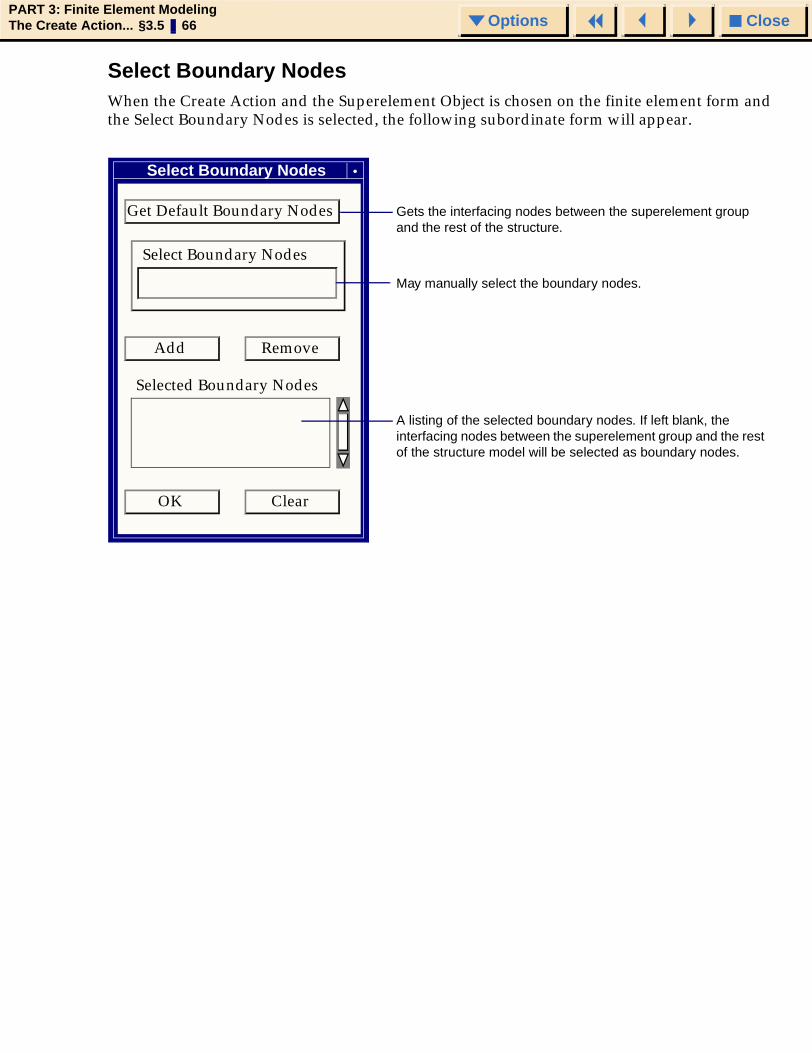
CloseOptionsPART 3: Finite Element ModelingThe Create Action... §3.5 66 Options
Select Boundary NodesWhen the Create Action and the Superelement Object is chosen on the finite element form and the Select Boundary Nodes is selected, the following subordinate form will appear.
Gets the interfacing nodes between the superelement group and the rest of the structure.
May manually select the boundary nodes.
A listing of the selected boundary nodes. If left blank, the interfacing nodes between the superelement group and the rest of the structure model will be selected as boundary nodes.
Select Boundary Nodes
Get Default Boundary Nodes
Select Boundary Nodes
Add Remove
Selected Boundary Nodes
OK Clear

CloseOptionsPART 3: Finite Element ModelingThe Create Action... §3.6 67 Options
3.6 Creating DOF ListDegree-of-Freedom (DOF) lists may be created by using this form and the subordinate form presented when Define Terms is selected. Note that this is currently available only for an ANSYS or ANSYS 5 analysis preference.
Specify a name for use in referencing the DOF list.
Shows all DOF lists that are currently defined in the database.
Finite Elements
Action: Create
Object: DOF List
Analysis Preferences: Code: ANSYS Type: Structural
DOF List Name
Available DOF Lists
Define Terms...

CloseOptionsPART 3: Finite Element ModelingThe Create Action... §3.6 68 Options
Define Terms
Displays the selected nodes and DOFs that were specified using the Node List databox and the DOFs listbox.
Highlight the degrees-of-freedom to be included in the DOFs cell of the degree-of-freedom list term.
Specify node IDs to be included in the nodes cell of the degree-of-freedom list.
Select option to Create, Modify or Delete entries in the degree-of-freedom list.
Selecting Clear will remove all terms from the degree-of-freedom list spreadsheet.
For Create or Modify, selecting Apply will either place the new term into the spreadsheet or replace the selected term with the modified term. For Delete, selecting Apply will delete the selected term.
Define Terms
Create Modify Delete
Node List
DOFs UX UY UZ
Apply Clear Cancel
Degree of Freedom List
Nodes DOFs
◆ ◆ ◆ ◆◆
AX RY RZ VOLT

CloseOptionsPART 3: Finite Element ModelingThe Transform Action § 69 Options
MSC.Patran Reference Manual, Part 3: Finite Element Modeling
CHAPTER
4 The Transform Action
■ Overview of Finite Element Modeling Transform Actions
■ Transforming Nodes
■ Transforming Elements

CloseOptionsPART 3: Finite Element ModelingThe Transform Action §4.1 70 Options
4.1 Overview of Finite Element Modeling Transform ActionsThe transformations described in the following sections are identical to their counterparts in ASM. The table below lists the objects (nodes and elements) and methods that are available when Transform is the selected Action.
Object Method
Node Translate
Rotate
Mirror
Element Translate
Rotate
Mirror
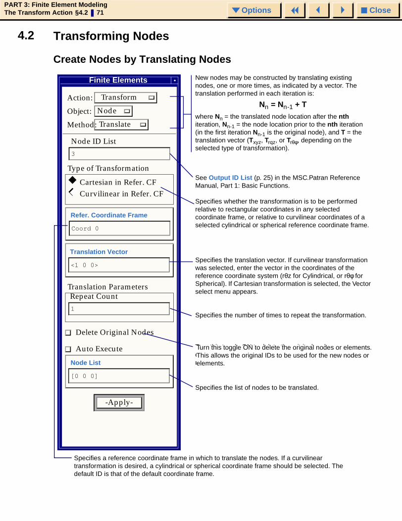
CloseOptionsPART 3: Finite Element ModelingThe Transform Action §4.2 71 Options
4.2 Transforming Nodes
Create Nodes by Translating Nodes
New nodes may be constructed by translating existing nodes, one or more times, as indicated by a vector. The translation performed in each iteration is:
Nn = Nn-1 + Twhere Nn = the translated node location after the nth iteration, Nn-1 = the node location prior to the nth iteration (in the first iteration Nn-1 is the original node), and T = the translation vector (Txyz, Trqz, or Trθφ, depending on the selected type of transformation).
Specifies whether the transformation is to be performed relative to rectangular coordinates in any selected coordinate frame, or relative to curvilinear coordinates of a selected cylindrical or spherical reference coordinate frame.
Specifies a reference coordinate frame in which to translate the nodes. If a curvilinear transformation is desired, a cylindrical or spherical coordinate frame should be selected. The default ID is that of the default coordinate frame.
Specifies the list of nodes to be translated.
Specifies the translation vector. If curvilinear transformation was selected, enter the vector in the coordinates of the reference coordinate system (rθz for Cylindrical, or rθφ for Spherical). If Cartesian transformation is selected, the Vector select menu appears.
Turn this toggle ON to delete the original nodes or elements. This allows the original IDs to be used for the new nodes or elements.
Specifies the number of times to repeat the transformation.
Finite Elements
Action: Transform
Object: Node
Method: Translate
Node ID List
3
Type of Transformation
Cartesian in Refer. CF Curvilinear in Refer. CF
Refer. Coordinate Frame
Coord 0
Translation Parameters Repeat Count
1
Delete Original Nodes
Auto Execute
Node List
[0 0 0]
-Apply-
Translation Vector
<1 0 0>
◆
◆◆
See Output ID List (p. 25) in the MSC.Patran Reference Manual, Part 1: Basic Functions.
Turn this toggle ON to delete the original nodes or elements. This allows the original IDs to be used for the new nodes or elements.

CloseOptionsPART 3: Finite Element ModelingThe Transform Action §4.2 72 Options
Create Nodes by Rotating Nodes
New nodes may be constructed by rotating nodes clockwise (CW) or counterclockwise (CCW) around an axis. The first rotation is specified as the sum of the Rotations Angle plus an offset. Any additional rotations (as specified by the Repeat Count parameter) are by the rotation angle only. The transformation performed for each iteration is:
1st Iteration: N1 = N0 + R(θo + θr)
Iterations 2 & up: Nn = Nn-1 + R(θn-1 + θr)
where N0 = the original node, N1 = the rotated location of node N0 after the first iteration, R = the radius of rotation,θo = the offset angle, θr = the rotation angle, Nn = the rotated location of a node after the nth iteration, Nn-1 = the node location prior to the nth iteration, and θn-1 = the angular displacement of node Nn-1 from the original node, N0.
θo
θr
N0Axis
θr
N1
Repeat Count = 2Radius
N2
The rotation plane is established by the axis and the node to rotate. The axis is a vector that is normal to the plane of rotation. The radius of rotation, a straight line in the plane of rotation, extends from the original node, N0, to the point of intersection with the projected extension of the axis.
Finite Elements
Action: Transform
Object: Node
Method: Rotate
Node ID List
3
Refer. Coordinate Frame
Coord 0
Axis
{[0 0 0][0 0 1]}
Rotation Parameters
Rotation Angle
90.0
Offset Angle
0.0
Repeat Count 1
Delete Original Nodes
Auto Execute
Node List
[0 0 0]
- Apply -

CloseOptionsPART 3: Finite Element ModelingThe Transform Action §4.2 73 Options
Specifies a reference coordinate frame in which to rotate the nodes. The default ID is that of the default coordinate frame. The Frame select menu appears.
Defines a vector normal to the plane of rotation. The Axis select menu appears.
Specifies the rotation angle, θr (in degrees) through which the nodes are to be rotated, default is 90 degrees CCW. Enter a negative angle if the rotation is to be CW.
Specifies the angular offset, θo, (in degrees), default is 0. Enter a negative angle if the offset is to be CCW.
Specifies the list of nodes to be rotated. The Node Select filter is in effect.
See Output ID List (p. 25) in the MSC.Patran Reference Manual, Part 1: Basic Functions.
Turn this toggle ON to delete the original nodes or elements. This allows the original IDs to be used for the new nodes or elements.
Specifies the number of times to repeat the transformation.
Finite Elements
Action: Transform
Object: Node
Method: Rotate
Node ID List
3
Refer. Coordinate Frame
Coord 0
Axis
{[0 0 0][0 0 1]}
Rotation Parameters
Rotation Angle
90.0
Offset Angle
0.0
Repeat Count 1
Delete Original Nodes
Auto Execute
Node List
[0 0 0]
-Apply-
Turn this toggle ON to delete the original nodes or elements. This allows the original IDs to be used for the new nodes or elements.

CloseOptionsPART 3: Finite Element ModelingThe Transform Action §4.2 74 Options
Create Nodes by Mirroring Nodes
Constructs new nodes by reflecting the listed nodes about a final mirror plane, that may be offset from a selected mirror plane. The transformation performed is as follows:
Nmirror = N0 - (2D)nwhere Nmirror = the location of the new node, and D = the distance (in the direction of vector n, which is normal to the final mirror plane) from the final mirror plane to the original node, N0.
The selected mirror plane can be any arbitrary plane in model space. If a nonzero offset, O, is specified, the final mirror plane used in the mirror action is offset from the selected mirror plane by the distance O in the direction of vector n.
Y Final Mirror PlaneSelected Mirror Plane (YZ)
Nmirror N0
D
Offset (O)
X
2D
In the example illustrated above, the selected mirror plane is the YZ plane of the global Cartesian coordinate system. Therefore, the offset and distance D are measured along the X axis (vector n), which is normal to the YZ plane.
Finite Elements
Action: Transform
Object:
Method:
Node
Mirror
Node ID List 3
Define Mirror Plane Normal
{[0 0 0][0 0 1]}
Offset Parameters Offset
0.0
Delete Original Nodes
Auto Execute
Node List
[0 0 0]
-Apply-

CloseOptionsPART 3: Finite Element ModelingThe Transform Action §4.2 75 Options
Specifies the normal to the plane that will serve as the selected mirror plane. The Axis select menu appears. The normal to the plane is defined by a vector, where the vector base originates in the plane, and the vector tip is normal to the plane.
Specifies offset of final mirror plane from selected mirror plane specified above. The offset is the distance (positive or negative), along the normal, from the selected mirror plane to the location of the final mirror plane.
Specifies the list of nodes to be mirrored. The Node Select filter is in effect.
See Output ID List (p. 25) in the MSC.Patran Reference Manual, Part 1: Basic Functions.
Turn this toggle ON to delete the original nodes or elements. This allows the original IDs to be used for the new nodes or elements.
Finite Elements
Action: Transform
Object:
Method:
Node
Mirror
Node ID List 3
Define Mirror Plane Normal
{[0 0 0][0 0 1]}
Offset Parameters Offset
0.0
Delete Original Nodes
Auto Execute
Node List
[0 0 0]
-Apply-

CloseOptionsPART 3: Finite Element ModelingThe Transform Action §4.3 76 Options
4.3 Transforming Elements
Create Elements by Translating Elements
Specifies whether the transformation is to be performed relative to rectangular coordinates in any selected coordinate frame, or relative to curvilinear coordinates of a selected cylindrical or spherical reference coordinate frame.
Specifies a reference coordinate frame in which to translate the elements. If a curvilinear transformation is desired, a cylindrical or spherical coordinate frame should be selected. The default ID is the same as the default coordinate frame.
Specifies the list of elements to be translated. The Element select menu appears.
Specifies the translation vector. If curvilinear transformation was selected, enter the vector in the coordinates of the reference coordinate system (rθz for Cylindrical, or rθφ for Spherical). If Cartesian transformation is selected, the Vector select menu appears.
See Output ID List (p. 25) in the MSC.Patran Reference Manual, Part 1: Basic Functions.
Turn this toggle ON to delete the original nodes or elements. This allows the original IDs to be used for the new nodes or elements.
Specifies the number of times to repeat the transformation.
Constructs new elements by performing a rigid-body or curvilinear (nonrigid body) translation, of each elements’ nodes, one or more times by an amount specified by a translation vector (number of iterations is determined by the Repeat Count).
An element is transformed by transforming each of its nodes. The result is exactly the same as if each of the nodes had been individually transformed.
Finite Elements
Action: Transform
Object: Object: Element
Method:
Translation Vector
<1 0 0>
Translate
Element ID List
1
Type of Transformation
Cartesian in Refer. CF Curvilinear in Refer. CF
Refer. Coordinate Frame
Coord 0
Translation Parameters
Repeat Count
1
Delete Original Elements
Auto Execute
Element List
-Apply-
◆
◆◆

CloseOptionsPART 3: Finite Element ModelingThe Transform Action §4.3 77 Options
Create Elements by Rotating Elements
Specifies a reference coordinate frame in which to rotate the elements. The default ID is that of the default coordinate frame. The Frame select menu appears.
Defines a vector normal to the plane of rotation. The Axis select menu appears.
Specifies the rotation angle, θr (in degrees), through which the elements are to be rotated default is 90 degrees CCW. Enter a negative angle if the rotation is to be CW.
Specifies the angular offset, θo (in degrees), default is 0. Enter a negative angle if the offset is to be CCW.
Specifies the list of elements to be rotated. The Element select menu appears.
See Output ID List (p. 25) in the MSC.Patran Reference Manual, Part 1: Basic Functions.
Turn this toggle ON to delete the original nodes or elements. This allows the original IDs to be used for the new nodes or elements.
Specifies the number of times to repeat the transformation.
Constructs new elements by performing a rigid-body rotation of each elements’ nodes one or more times by an amount specified by a rotation angle (number of iterations is determined by the Repeat Count).
An element is transformed by transforming each of its nodes. The result is exactly the same as if each of the nodes had been individually transformed.
Finite Elements
Action: Transform
Object: Element
Method: Rotate
Element ID List
1
Refer. Coordinate Frame
Coord 0
Axis
{[0 0 0][0 0 1]}
Rotation Parameters Rotation Angle
90.0
Offset Angle
0.0
Repeat Count
1
Delete Original Elements
Auto Execute
Element List
-Apply-

CloseOptionsPART 3: Finite Element ModelingThe Transform Action §4.3 78 Options
Create Elements by Mirroring Elements
Specifies the normal to the plane that is to serve as the selected mirror plane. Axis select menu appears. The normal to the plane is defined by a vector where the vector base originates in the plane and the vector tip is normal to the plane.
Specifies offset of final mirror plane from selected mirror plane specified above. The offset is the distance (positive or negative), along the normal, from the selected mirror plane to the location of the final mirror plane.
Specifies the list of elements to be mirrored. The Element select menu appears.
See Output ID List (p. 25) in the MSC.Patran Reference Manual, Part 1: Basic Functions.
Turn this toggle ON to delete the original nodes or elements. This allows the original IDs to be used for the new nodes or elements.
Constructs new elements by reflecting each element’s nodes about a final mirror plane that may be offset form a selected mirror plane.
An element is transformed by transforming each of its nodes. The result is exactly the same as if each of the nodes had been individually transformed.
If ON, the element connectivity will be reversed. Reversing elements ensures that shell elements have consistent normals, and that solid elements have positive volumes. (Note: Negative volume elements will not be created under any circumstances.)
Finite Elements
Action: Transform
Object:
Method:
Element
Mirror
Element ID List
1
Define Mirror Plane Normal
{[0 0 0][0 0 1]}
Offset Parameters Offset
0.0
Reverse Elements
Delete Original Elements
Auto Execute
Element ID List
-Apply-

CloseOptionsPART 3: Finite Element ModelingThe Sweep Action § 79 Options
MSC.Patran Reference Manual, Part 3: Finite Element Modeling
CHAPTER
5 The Sweep Action
■ Introduction
■ Sweep Forms

CloseOptionsPART 3: Finite Element ModelingThe Sweep Action §5.1 80 Options
5.1 IntroductionSweeping elements is the process of creating higher order elements by sweeping a lower order element through a prescribed path. Therefore, a hex element may be created by sweeping a quad element through space, the edges of the hex being defined by the corners of the quad as its nodes move along the path. Ten methods for defining the swept paths are provided: Arc, Extrude, Glide, Glide-Guide, Normal, Radial Cylindrical, Radial Spherical, Spherical Theta, Vector Field and Loft.

CloseOptionsPART 3: Finite Element ModelingThe Sweep Action §5.2 81 Options
5.2 Sweep FormsThe following options are available when Sweep is the selected Action and Element is the selected Object.
Method Description
Arc The Arc method allows the creation of one or more elements by sweeping a surface element about an axis of rotation.
Extrude The Extrude method allows creation of one or more elements by moving a base element through space along a defined vector.
Glide The Glide method allows the creation of one or more elements by sweeping the base element along the path of a glide curve.
Glide-Guide The Glide-Guide method allows the creation of one or more elements by sweeping the base element along the path of a glide curve, while the orientation with respect to the base is determined by means of a guide curve.
Normal The Normal method allows creation of one or more elements by sweeping a base of element in a normal direction.
Radial Cylindrical The Radial Cylindrical method allows creation of one or more elements by sweeping the base element through space radially outward from a center axis.
Radial Spherical The Radial Spherical method allows creation of one or more elements by sweeping the base element through space radially outward from a center point.
Spherical Theta The Spherical Theta method allows creation of one or more elements by sweeping the base element through space along a path on a sphere that is like sweeping in the latitude direction in the earth’s latitude and longitude system.
Vector Field The Vector Field method allows creation of one or more elements by sweeping a base element in a direction as determined by evaluating a vector field at each of the base nodes.
Loft The Loft method allows creation of one or more elements by sweeping a 2D base element to the location of a 2D top element. The two meshes have to be topological congruent.

CloseOptionsPART 3: Finite Element ModelingThe Sweep Action §5.2 82 Options
The Arc MethodThe Arc method allows the creation of one or more elements by sweeping base entities about an axis of rotation, as shown below. The element edge length in the swept direction is defined explicitly, similar to creating a mesh seed for the meshing function.
Specifies Output ID List (p. 25) in the MSC.Patran Reference Manual, Part 1: Basic Functions for elements and nodes
Brings up the FE Parameters form. Use to define optional parameters for the elements to be swept. Normally, the default settings do not need to be modified.
Brings up the Mesh Control form. Use to define mesh control parameters. Initially, this form is raised because it contains required information.
Specifies the Reference Coordinate Frame where the Axis Vector is defined. The default ID is that of the active coordinate frame.
Specifies the axis of rotation by defining a vector normal to the plane of rotation.
Specifies a positive or negative rotation angle (θr), in degrees, through which the elements are to be swept. Direction of the rotation is determined by the right hand rule. Negative angles may be specified.
Toggle ON to delete base elements after the sweep. Nodes which are not used by other elements are also deleted. Element faces and edges, which may be in the base entity list, are not affected by this toggle.
Specifies a list of base entities to be swept.
θr
Arc
Base Elemen
Axis
Specifies an angular offset, in degrees, for the initial base locations. Negative offset angles may be specified.
Finite Elements
Action: Sweep
Object:
Method:
Element
Arc
Output IDs
Element ID List
1
Node ID List
1
FE Parameters ...
Mesh Control ...
Refer. Coordinate Frame
Coord 0
Axis
{[0 0 0][0 0 1]}
Sweep Angle
90.0
Offset
0.0
Delete Original Elements
Base Entity List
-Apply-

CloseOptionsPART 3: Finite Element ModelingThe Sweep Action §5.2 83 Options
The Extrude MethodThe Extrude method allows creation of one or more elements by moving a base entities through space along a defined vector. The extrusion vector is applied to each listed entity.
Specifies Output ID List (p. 25) in the MSC.Patran Reference Manual, Part 1: Basic Functions for nodes and elements to be created.
Brings up the FE Parameters form. Use to define optional parameters for the elements to be swept. Normally, the default settings do not need to be modified.
Specifies the Reference Coordinate Frame in which the Direction Vector is defined. The default ID is the same as the active coordinate frame.
Specifies the direction of the translation. When the direction vector is changed, the Magnitude databox is automatically loaded with the corresponding magnitude of the new vector.
Specifies the distance to extrude along the direction vector. This value is automatically loaded when the direction vector is changed. If negative the sweep will occur in the opposite direction of the direction vector.
Specifies a list of entities which are to be swept.
Brings up the Mesh Control form. Use to define mesh control parameters. Initially, this form is raised because it contains required information.
Specifies an offset for the initial base locations. Negative offsets may be specified.
Toggle ON to delete base elements after the sweep. Nodes which are not used by other elements are also deleted. Element faces and edges, which may be in the base entity list, are not affected by this toggle.
Finite Elements
Action: Sweep
Method:
Object: Element
Extrude
Output IDs Element ID List1
Node ID List 1
FE Parameters ...
Mesh Control ...
Refer. Coordinate Frame
Coord 0
Direction Vector
<0 0 -2>
Extrude Distance4.
Offset 0.0
Delete Original Elements
Base Entity List
Eml 4
-Apply-
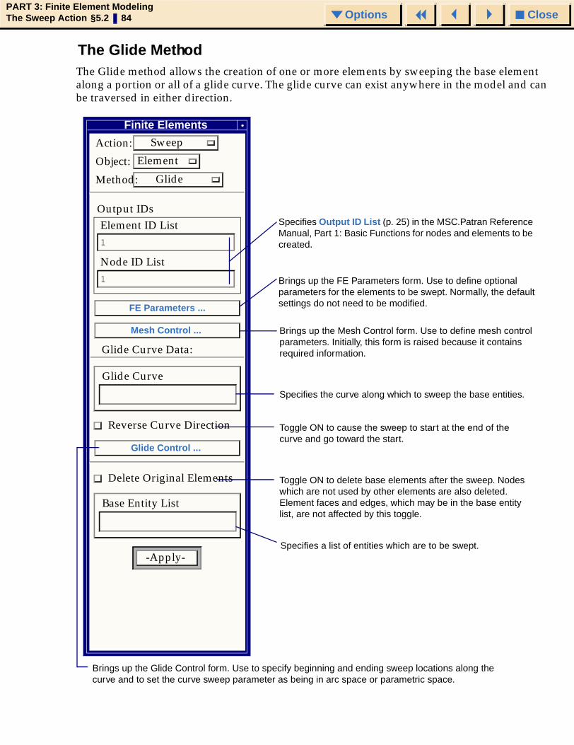
CloseOptionsPART 3: Finite Element ModelingThe Sweep Action §5.2 84 Options
The Glide MethodThe Glide method allows the creation of one or more elements by sweeping the base element along a portion or all of a glide curve. The glide curve can exist anywhere in the model and can be traversed in either direction.
Specifies the curve along which to sweep the base entities.
Brings up the Glide Control form. Use to specify beginning and ending sweep locations along the curve and to set the curve sweep parameter as being in arc space or parametric space.
Specifies Output ID List (p. 25) in the MSC.Patran Reference Manual, Part 1: Basic Functions for nodes and elements to be created.
Brings up the FE Parameters form. Use to define optional parameters for the elements to be swept. Normally, the default settings do not need to be modified.
Brings up the Mesh Control form. Use to define mesh control parameters. Initially, this form is raised because it contains required information.
Specifies a list of entities which are to be swept.
Toggle ON to delete base elements after the sweep. Nodes which are not used by other elements are also deleted. Element faces and edges, which may be in the base entity list, are not affected by this toggle.
Toggle ON to cause the sweep to start at the end of the curve and go toward the start.
Finite Elements
Action: Sweep
Method:
Object: Element
Glide
Output IDs Element ID List 1
Node ID List 1
FE Parameters ...
Mesh Control ...
Glide Curve Data:
Glide Curve
Reverse Curve Direction
Glide Control ...
Delete Original Elements
Base Entity List
-Apply-

CloseOptionsPART 3: Finite Element ModelingThe Sweep Action §5.2 85 Options
Glide Control
The Glide Control allows curves in the model to be used without having to perform simple operations such as break and translate. It also allows for sweeping to be done in arc length or parametric coordinates along the curve.
Toggles whether space or parametric coordinate system is used to specify the beginning and ending points below.
Offset from begin/end of curve to begin point. Swept mesh begins at begin point and proceeds to the end point.
Toggle Curve Sweep Parameter. Specifies whether mesh seeding is done in units of arc length or curve parameterization.
Beginning and Ending points on curve along which to do the sweep. If the Parametric Coordinates are toggled on above, these are entered as parametric values on the curve. Points can be in any order along curve. Beginning and ending points on curve are used by default if left blank.
Specifies the Reference Coordinate Frame in which the Beginning and Ending Points are defined. The default ID is the same as the active coordinate frame. This is only used when Space Coordinates is the selected system.
Glide Control
Point Coordinate System
Space Coordinates
Parametric Coordinates
Refer. Coordinate Frame
Coord 0
Glide Begin Point
Glide End Point
Offset to Glide Beginning
Curve Sweep Parameter
Arc Length
Curve Parameterization
OK
◆
◆◆
◆◆
◆
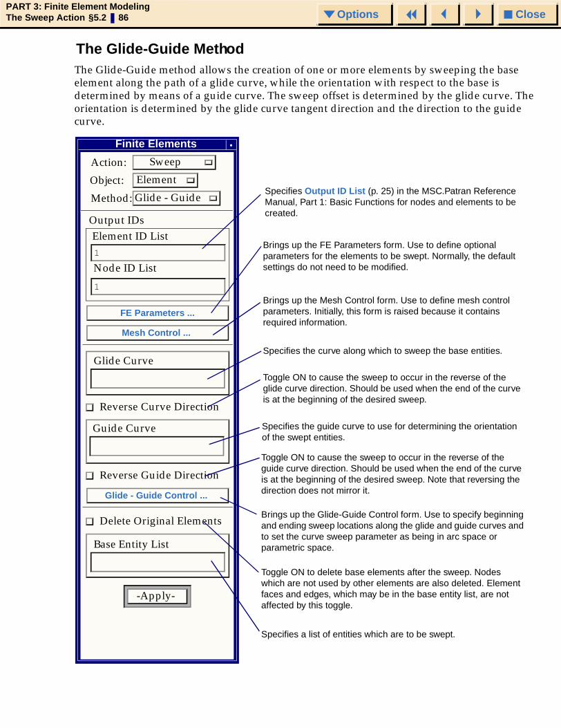
CloseOptionsPART 3: Finite Element ModelingThe Sweep Action §5.2 86 Options
The Glide-Guide MethodThe Glide-Guide method allows the creation of one or more elements by sweeping the base element along the path of a glide curve, while the orientation with respect to the base is determined by means of a guide curve. The sweep offset is determined by the glide curve. The orientation is determined by the glide curve tangent direction and the direction to the guide curve.
Brings up the FE Parameters form. Use to define optional parameters for the elements to be swept. Normally, the default settings do not need to be modified.
Brings up the Mesh Control form. Use to define mesh control parameters. Initially, this form is raised because it contains required information.
Specifies Output ID List (p. 25) in the MSC.Patran Reference Manual, Part 1: Basic Functions for nodes and elements to be created.
Toggle ON to cause the sweep to occur in the reverse of the glide curve direction. Should be used when the end of the curve is at the beginning of the desired sweep.
Specifies a list of entities which are to be swept.
Toggle ON to delete base elements after the sweep. Nodes which are not used by other elements are also deleted. Element faces and edges, which may be in the base entity list, are not affected by this toggle.
Brings up the Glide-Guide Control form. Use to specify beginning and ending sweep locations along the glide and guide curves and to set the curve sweep parameter as being in arc space or parametric space.
Toggle ON to cause the sweep to occur in the reverse of the guide curve direction. Should be used when the end of the curve is at the beginning of the desired sweep. Note that reversing the direction does not mirror it.
Specifies the guide curve to use for determining the orientation of the swept entities.
Specifies the curve along which to sweep the base entities.
Finite Elements
Action: Sweep
Object:
Method:
Node ID List
Pattern:Pattern:Pattern:
Element
Glide - Guide
Output IDs Element ID List 1
1
FE Parameters ...
Mesh Control ...
Glide Curve
Reverse Curve Direction
Guide Curve
Reverse Guide Direction
Glide - Guide Control ...
Delete Original Elements
Base Entity List
-Apply-

CloseOptionsPART 3: Finite Element ModelingThe Sweep Action §5.2 87 Options
The Glide-Guide method allows sweeps to be swept and rotated along a desired path. One good application of this method is that of meshing a pipe as it goes around a bend.
For this example, the base entities are a quad mesh on the cross section of a pipe. The glide curve is curve 1 and the guide curve is curve 2. The glide curve can be thought of as the top seam of the pipe. In this case, the guide curve is along the bottom seam of the pipe. The centerline of the pipe could just as easily been used.
Although only a 90-degree bend is shown here, the glide and guide curves are not limited to a specified angle or number of bends.
Before:
After:

CloseOptionsPART 3: Finite Element ModelingThe Sweep Action §5.2 88 Options
Glide-Guide Control
The Glide-Guide Control allows curves in the model to be used without having to perform simple operations such as break and translate. It also allows for sweeping to be done in arc length or parametric coordinates along the curve. Note that for Glide-Guide, the beginning or end of the curves should touch the base elements for best results. Otherwise, undesirable results may occur due to the large effect of orientation’s rotations on the base entities.
Offset from begin/end of curve to begin point. Swept mesh begins at begin point.
Toggle curve sweep parameter. Specifies whether mesh seeding is done in units of arc length or curve parameterization.
Beginning and ending points on curve along which to do the sweep. If the Parametric Coordinates are toggled on above, these are entered as parametric values on the curve. Points can be in any order along curve.
Specifies the Reference Coordinate Frame in which the beginning and ending points are defined. The default ID is the same as the active coordinate frame. This is only used when Space Coordinates is one of the selected systems.
Toggles local axis to be preserved as the sweep progresses and the orientation changes along the glide and guide curves.
Toggle type of coordinates to use to specify the beginning and ending points below.
Glide - Guide Control
Refer. Coordinate Frame
Coord 0
Glide Frame Orientation
Preserve Glide Tangent Preserve Guide Direction
Glide Curve: Guide Curve:
Point Coordinate System
Space Coordinates Parametric Coordinates
Point Coordinate System
Space Coordinates Parametric Coordinates
Glide Begin Point
Glide End Point
Guide Begin Point
Guide End Point
Offset to Glide Beginning Offset to Guide Beginning
Curve Sweep Parameter
Arc Length Curve Parameterization
Guide Sweep Parameter
Arc Length Curve Parameterization
OK
◆
◆◆
◆
◆◆
◆
◆◆
◆
◆◆
◆
◆◆

CloseOptionsPART 3: Finite Element ModelingThe Sweep Action §5.2 89 Options
The Normal MethodThe Normal method allows creation of one or more elements by sweeping base entities in a normal direction. If the base elements are associated with geometry, the normal direction for each node will be the surface normal at that location. If the elements are unassociated, the normal direction will be the average of the element normals of all the elements in the base entity list referencing the node.
For unassociated base elements, the normals must be consistent. If not, an error is reported and execution terminated.
Specifies Output ID List (p. 25) in the MSC.Patran Reference Manual, Part 1: Basic Functions for the nodes and elements to be created.
Specifies the sweep distance. If negative the sweep will occur in the opposite direction of the normal vector.
Toggle ON to cause the sweep to occur in the opposite direction indicated by the sign of the Normal Length parameter.
Specifies a list of entities which are to be swept.
Brings up the FE Parameters form. Use to define optional parameters for the elements to be swept. Normally, the default settings do not need to be modified.
Brings up the Mesh Control form. Use to define mesh control parameters. Initially, this form is raised because it contains required information.
Specifies an offset for the initial base locations. Negative offsets may be specified.
Toggle ON to delete base elements after the sweep. Nodes which are not used by other elements are also deleted. Element faces and edges, which may be in the base entity list, are not affected by this toggle.
Finite Elements
Action: Sweep
Object:
Method:
Element
Normal
Output IDs Element ID List
Node ID List 18
FE Parameters ...
Mesh Control ...
Normal Length 1.0
Offset 0.0
Reverse Normal Direction
Delete Original Elements
Base Entity List
-Apply-

CloseOptionsPART 3: Finite Element ModelingThe Sweep Action §5.2 90 Options
The Radial Cylindrical MethodThe Radial Cylindrical method allows creation of one or more elements by sweeping the base element through space radially outward from a center axis.
Specifies Output ID List (p. 25) in the MSC.Patran Reference Manual, Part 1: Basic Functions for nodes and elements to be created.
Brings up the FE Parameters form. Use to define optional parameters for the elements to be swept. Normally, the default settings do not need to be modified.
Brings up the Mesh Control form. Use to define mesh control parameters. Initially, this form is raised because it contains required information.
Specifies the Reference Coordinate Frame in which the Axis is defined. The default ID is the same as the active coordinate frame.
Specifies the cylindrical axis. All elements are swept out from this central axis.
Total distance to sweep in radial direction from axis.
Distance to offset in radial direction from axis before starting sweep.
Specifies a list of entities which are to be swept.
Toggle ON to delete base elements after the sweep. Nodes which are not used by other elements are also deleted. Element faces and edges, which may be in the base entity list, are not affected by this toggle.
Finite Elements
Action: Sweep
Object:
Method:
Element
Radial Cyl.
Output IDs
Element ID List 1
Node ID List 1
FE Parameters ...
Mesh Control ...
Refer. Coordinate Frame
Coord 0
Axis
Coord 0.3
Radial Distance
1.0
Offset
0.0
Delete Original Elements
Base Entity List
-Apply-

CloseOptionsPART 3: Finite Element ModelingThe Sweep Action §5.2 91 Options
The Radial Spherical MethodThe Radial Spherical method allows creation of one or more elements by sweeping the base element through space radially outward from a center point.
Specifies a list of entities which are to be swept.
Toggle ON to delete base elements after the sweep. Nodes which are not used by other elements are also deleted. Element faces and edges, which may be in the base entity list, are not affected by this toggle.
Total distance to sweep out from sphere center point.
Offset distance in radial direction to beginning of sweep.
Specifies Output ID List (p. 25) in the MSC.Patran Reference Manual, Part 1: Basic Functions for nodes and elements to be created.
Brings up the FE Parameters form. Use to define optional parameters for the elements to be swept. Normally, the default settings do not need to be modified.
Brings up the Mesh Control form. Use to define mesh control parameters. Initially this form is raised because it contains required information.
Specifies the sphere center point. All elements are swept out from this center point.
Specifies the Reference Coordinate Frame in which the Sphere Center Point is defined. The default ID is the same as the active coordinate frame.
Finite Elements
Action: Sweep
Object:
Method:
Element
Radial Sph.
Output IDs Element ID List
1
Node ID List
1
FE Parameters ...
Mesh Control ...
Refer. Coordinate Frame
Coord 0
Sphere Center Point
[0 0 0]
Radial Distance
1.0
Offset
0.0
Delete Original Elements
Base Entity List
-Apply-

CloseOptionsPART 3: Finite Element ModelingThe Sweep Action §5.2 92 Options
The Spherical Theta MethodThe Spherical Theta method allows creation of one or more elements by sweeping the base element through space along a path on a sphere that is like sweeping in the latitude direction in the earth’s latitude and longitude system.
Finite Elements
Specifies Output ID List (p. 25) in the MSC.Patran Reference Manual, Part 1: Basic Functions for nodes and elements to be created.
Brings up the FE Parameters form. Use to define optional parameters for the elements to be swept. Normally, the default settings do not need to be modified.
Brings up the Mesh Control form. Use to define mesh control parameters. Initially, this form is raised because it contains required information.
Specifies the Reference Coordinate Frame in which the Sphere Center Point is defined. The default ID is the same as the active coordinate frame.
Specifies a list of entities which are to be swept.
Toggle ON to delete base elements after the sweep. Nodes which are not used by other elements are also deleted. Element faces and edges, which may be in the base entity list, are not affected by this toggle.
Specifies the offset angle, in degrees, to offset before beginning sweep.
Specifies the angle, in degrees, to sweep the elements, with the positive direction being from the “north” pole towards the “equator” of the spherical system.
Specifies the spherical center point and a direction to the “north pole” of the sphere. All elements are swept in the spherical theta direction with respect to this axis.
Finite Elements
Action: Sweep
Object:
Method:
Element
Sph. Theta
Output IDs
Element ID List 1
Node ID List 1
FE Parameters ...
Mesh Control ...
Refer. Coordinate Frame
Coord 0
Axis, Base at Sph. Center
Coord 0.3
Sweep Angle
45.0
Offset
0.0
Delete Original Elements
Base Entity List
-Apply-

CloseOptionsPART 3: Finite Element ModelingThe Sweep Action §5.2 93 Options
The following is an example of how the spherical theta method can be used to mesh a section of a hollow sphere:
The base entities are first set up. In this case, they are quads on a patch that is in the x-y plane. The default axis was used for this sweep (i.e., [0 0 0][0 0 1]). Therefore, the reference sphere for the sweeping process is one that is centered at the origin and has its pole along the z-axis.
The sweep direction is from the pole (in this case, the z-axis) toward the south pole, thereby creating a section of a hollow sphere.
Before:
After:
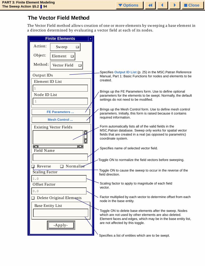
CloseOptionsPART 3: Finite Element ModelingThe Sweep Action §5.2 94 Options
The Vector Field MethodThe Vector Field method allows creation of one or more elements by sweeping a base element in a direction determined by evaluating a vector field at each of its nodes.
Specifies name of selected vector field.
Toggle ON to cause the sweep to occur in the reverse of the field direction.
Factor multiplied by each vector to determine offset from each node in the base entity.
Specifies Output ID List (p. 25) in the MSC.Patran Reference Manual, Part 1: Basic Functions for nodes and elements to be created.
Brings up the FE Parameters form. Use to define optional parameters for the elements to be swept. Normally, the default settings do not need to be modified.
Brings up the Mesh Control form. Use to define mesh control parameters. Initially, this form is raised because it contains required information.
Toggle ON to normalize the field vectors before sweeping.
Scaling factor to apply to magnitude of each field vector.
Specifies a list of entities which are to be swept.
Toggle ON to delete base elements after the sweep. Nodes which are not used by other elements are also deleted. Element faces and edges, which may be in the base entity list, are not affected by this toggle.
Finite Elements
Action: Sweep
Pattern:Pattern:Pattern:
Object: Element
Method: Vector Field
Output IDs
Element ID List
1
Node ID List
FE Parameters ...
Mesh Control ...
Existing Vector Fields
Field Name
Reverse Normalize Scaling Factor
1.0
Offset Factor
0.0
Delete Original Elements
Base Entity List
-Apply-
Form automatically lists all of the valid fields in the MSC.Patran database. Sweep only works for spatial vector fields that are created in a real (as opposed to parametric) coordinate system.
1

CloseOptionsPART 3: Finite Element ModelingThe Sweep Action §5.2 95 Options
The following is an example of how the vector field sweep could be used:
The base entities are quads in the x-y plane. The underlying patch measures 2*PI units in the x direction and 1 unit in the y direction. The following vector field is used:
X = 0.0
Y = 0.0
Z = 1.5 + COS(X)
This field is evaluated at each of the base nodes to determine both the sweep direction and total sweep distance.
The mesh control is set for this example to create 4 equally sized elements in the direction of the sweep. The resulting mesh represents a cosine wave.
Although an equation was used to create the field (see Spatial Field (p. 140) in the MSC.Patran Reference Manual, Part 5: Functional Assignments), other means can be used, such as filling in a table of data.
Before:
After:

CloseOptionsPART 3: Finite Element ModelingThe Sweep Action §5.2 96 Options
The Loft MethodThe Loft method allows creation of one or more elements by sweeping a 2D base element to the location of a 2D top element. The two meshes have to be topological congruent.
Specify a start element in first and second list. These two elements will be the first to be connected. If no elements are specified the first element in the entity lists will be used as a start element.
Specifies a list of 2D elements which are to be swept. The first and second entity list defines two meshes, which will be connected with 3D elements. The number of elements in these two boxes has to be the same.
Toggle ON to delete base and top elements after the sweep. Nodes which are not used by other elements are also deleted.
Specifies Output ID List (p. 25) in the MSC.Patran Reference Manual, Part 1: Basic Functions for nodes and elements to be created.
Brings up the FE Parameters form. Use to define optional parameters for the elements to be swept. Normally, the default settings do not need to be modified.
Brings up the Mesh Control form. Use to define mesh control parameters. Initially this form is raised because it contains required information.
Finite Elements
Action: Sweep
Method:
Pattern:Pattern:Pattern:
Object: Element
Loft
Output IDs
Element ID List
1
Node ID List
1
FE Parameters ...
Mesh Control ...
Auto Align Start Elements
Delete Original Elements
Auto Execute
First Entity List
Second Entity List
Start Element in First List
Start Element in Second List
-Apply-

CloseOptionsPART 3: Finite Element ModelingThe Sweep Action §5.2 97 Options
FEM Data
This form appears when the FE Parameters button is selected on any of the Sweep forms.
Specifies the type of element to be swept from each base element type listed.
Specifies the Analysis Coordinate Frame for all of the swept nodes.
Specifies the Reference Coordinate Frame for all of the swept nodes.
Sweep FEM Parameters Sweep Topologies:
Point: Bar2
Bar2: Quad4
Analysis Coordinate Frame
Coord 0
Refer. Coordinate Frame
Coord 0
OK
Results Displacement Offset
Select Results Case...
Select Displacement Result...
Select Layer...
This feature, when turned ON, allows you to sweep elements based on rezoned nodal/element locations from displacement results of a previously run analysis.
For example, say you run an axisymmetric analysis of a wheel. From the displaced results of the axisymmetric model you want to create a full 3D model of the wheel to run subsequent analyses but from the deformed state of the axisymmetric analysis. To do this, you would Select the Results Case... of the axisymmetric model and then Select the Displacement Result... from which you want to create the rezoned mesh. (If multiple layers of results exist, you will have to Select the appropriate Layer... also.)
Naturally the results must exist in the database to perform this rezoned sweep. All sweep commands can use rezoning from displacement results except Method = Loft.
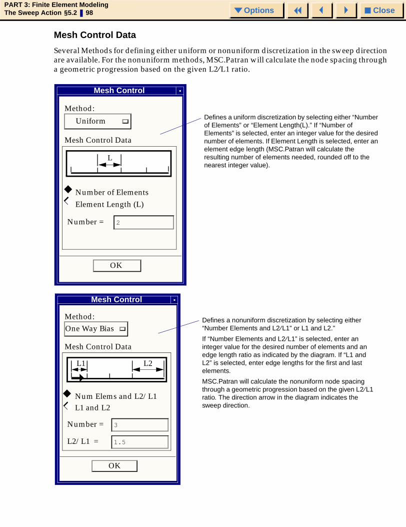
CloseOptionsPART 3: Finite Element ModelingThe Sweep Action §5.2 98 Options
Mesh Control Data
Several Methods for defining either uniform or nonuniform discretization in the sweep direction are available. For the nonuniform methods, MSC.Patran will calculate the node spacing through a geometric progression based on the given L2 ⁄L1 ratio.
Defines a uniform discretization by selecting either “Number of Elements” or “Element Length(L).” If “Number of Elements” is selected, enter an integer value for the desired number of elements. If Element Length is selected, enter an element edge length (MSC.Patran will calculate the resulting number of elements needed, rounded off to the nearest integer value).
Mesh Control
Method:
Uniform
Mesh Control Data
Number of Elements Element Length (L)
Number = 2
OK
L
◆
◆◆
Defines a nonuniform discretization by selecting either “Number Elements and L2 ⁄L1” or L1 and L2.”
If “Number Elements and L2 ⁄L1” is selected, enter an integer value for the desired number of elements and an edge length ratio as indicated by the diagram. If “L1 and L2” is selected, enter edge lengths for the first and last elements.
MSC.Patran will calculate the nonuniform node spacing through a geometric progression based on the given L2 ⁄L1 ratio. The direction arrow in the diagram indicates the sweep direction.
Mesh Control
Method: One Way Bias
Mesh Control Data
Num Elems and L2/L1 L1 and L2
Number = 3
L2/L1 = 1.5
OK
L2L1
◆
◆◆
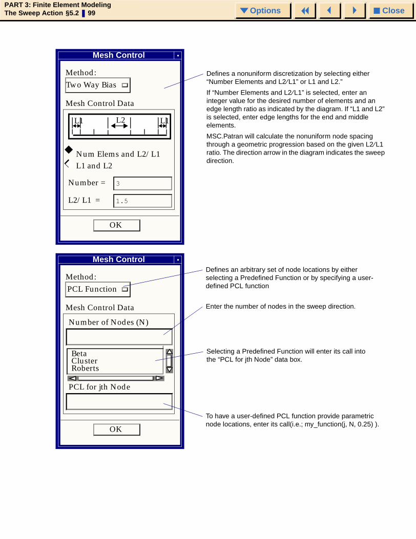
CloseOptionsPART 3: Finite Element ModelingThe Sweep Action §5.2 99 Options
Defines a nonuniform discretization by selecting either “Number Elements and L2 ⁄L1” or L1 and L2.”
If “Number Elements and L2 ⁄L1” is selected, enter an integer value for the desired number of elements and an edge length ratio as indicated by the diagram. If “L1 and L2” is selected, enter edge lengths for the end and middle elements.
MSC.Patran will calculate the nonuniform node spacing through a geometric progression based on the given L2 ⁄L1 ratio. The direction arrow in the diagram indicates the sweep direction.
Mesh Control
Method: Two Way Bias
Mesh Control Data
Num Elems and L2/L1 L1 and L2
Number = 3
L2/L1 = 1.5
OK
L2L1 L1
◆
◆◆
Enter the number of nodes in the sweep direction.
Mesh Control
Method: PCL Function
Mesh Control Data
OK
Number of Nodes (N)
PCL for jth Node
BetaClusterRoberts
Selecting a Predefined Function will enter its call into the “PCL for jth Node” data box.
To have a user-defined PCL function provide parametric node locations, enter its call(i.e.; my_function(j, N, 0.25) ).
Defines an arbitrary set of node locations by either selecting a Predefined Function or by specifying a user-defined PCL function

CloseOptionsPART 3: Finite Element ModelingThe Sweep Action §5.2 100 Options

CloseOptionsPART 3: Finite Element ModelingThe Renumber Action § 101 Options
MSC.Patran Reference Manual, Part 3: Finite Element Modeling
CHAPTER
6 The Renumber Action
■ Introduction
■ Renumber Forms

CloseOptionsPART 3: Finite Element ModelingThe Renumber Action §6.1 102 Options
6.1 IntroductionMost often, ID numbers (IDs) for finite element nodes and elements are chosen and assigned automatically. The Renumber Action permits the IDs of nodes and elements to be changed. This capability is useful to:
• Offset the IDs of a specific list of entities.
• Renumber the IDs of all existing entities within a specified range.
• Compact the IDs of an entity type sequentially from 1 to N.
IDs must be positive integers. Duplicate IDs are not permitted in the List of New IDs, or in the selected Entity List (old IDs). A Starting ID or a List of New IDs may be entered in the input databox. If a finite element entity outside the list of entities being renumbered is using the new ID, the renumber process will abort since each entity must have a unique ID. The default is to renumber all the existing entities beginning with the minimum ID through the maximum ID consecutively starting with 1.
If only one ID is entered, it is assumed to be the starting ID. The entities will be renumbered consecutively beginning with the starting ID.
If more than one ID is entered, then there must be at least as many new IDs as there are valid old IDs. If there are fewer IDs in the List of New IDs than there are valid IDs in the selected Entity List, renumbering will not take place and a message will appear in the command line indicating exactly how many IDs are needed. The List of New IDs may not contain a #. However, the list may have more IDs than needed.
The IDs in the selected Entity List may contain a #. The value of the maximum existing ID is automatically substituted for the #. There may be gaps of nonexisting entities in the list but there must be at least one valid entity ID in order for renumbering to take place.
A percent complete form shows the status of the renumber process. When renumbering is complete, a report appears in the command line indicating the number of entities renumbered and their new IDs. The renumber process may be halted at any time by pressing the Abort button and the old IDs will be restored.
Important: Try to estimate the number of IDs needed. A large number of unnecessary IDs will slow down the renumber process.

CloseOptionsPART 3: Finite Element ModelingThe Renumber Action §6.2 103 Options
6.2 Renumber FormsWhen Renumber is the selected Action the following options are available.
Object Description
Node The node menu selection provides the capability to renumber or change the IDS of nodes.
Element The element menu selection provides the capability to renumber or change the IDs of elements.

CloseOptionsPART 3: Finite Element ModelingThe Renumber Action §6.2 104 Options
Renumber NodesFigure 6-1
Use this option to renumber nodes. Each node has a unique node ID. See Introduction (p. 102).
Shows how many nodes exist in the model and minimum ⁄maximum values of node IDs. Note: All nodes are numbered sequentially when the Maximum ID is equal to Total in Model.
Specifies the starting ID, or a list of new node IDs to assign. Node IDs must be positive integers. Although # is not a valid entry here, a large number may be entered. If the number of IDs is less than the number of valid nodes, renumbering will not take place.
Specifies which old nodes are to be renumbered. A list of nodes can be entered here or an active group of nodes can be selected from the viewport.
The default is to renumber all nodes (Node minimum ID to maximum ID) consecutively beginning with the Start ID. The entry, Node 1:#, is also valid to indicate all nodes. There may be gaps of nonexisting nodes in the list, but there must be at least one valid node in order for renumbering to take place. Duplicate IDs are not permitted.
If a node outside the list of nodes being renumbered is using the new ID, the renumber process will abort since each node must have a unique ID.
Finite Elements Action: Renumber
Object:
Node
Node Summary
Total in Model: 2713
Minimum ID 21
Maximum ID 2733
Start ID or List of New IDs
1
Node List-Apply-
Node List
Node 21:2733
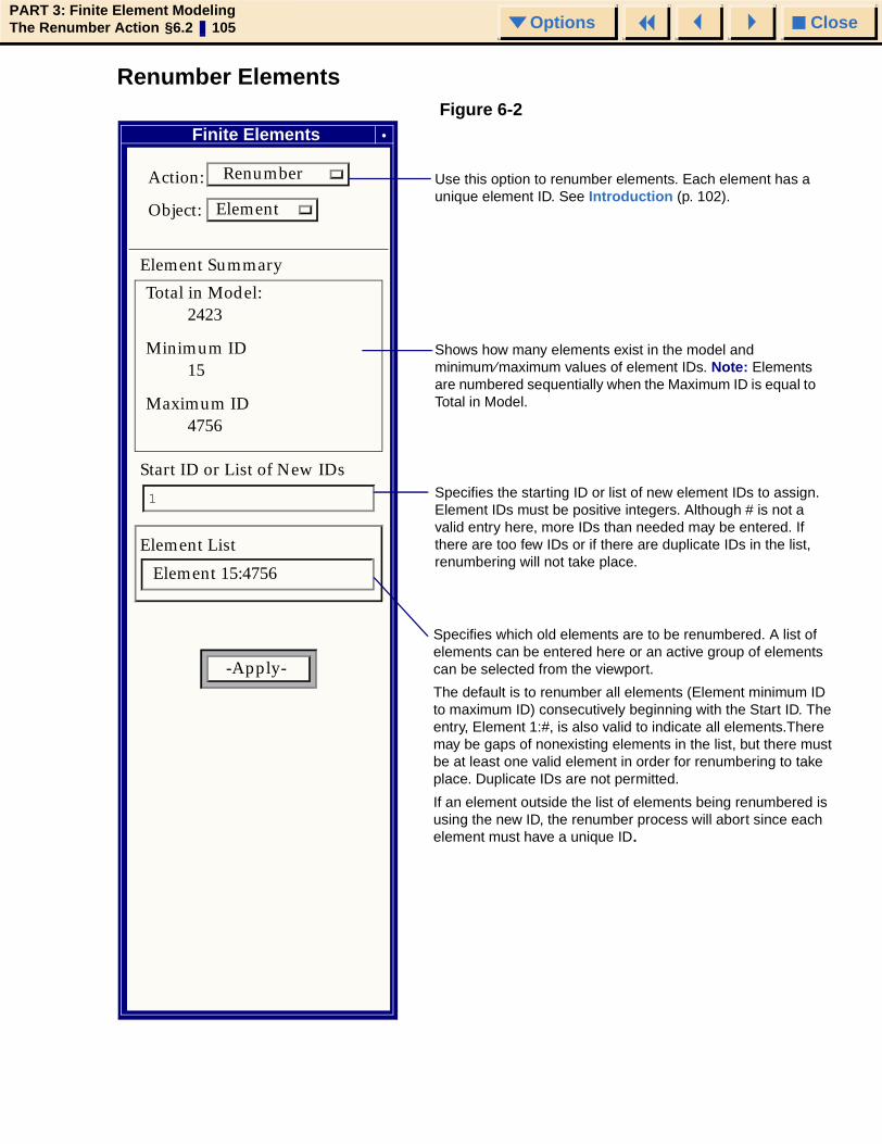
CloseOptionsPART 3: Finite Element ModelingThe Renumber Action §6.2 105 Options
Renumber ElementsFigure 6-2
Use this option to renumber elements. Each element has a unique element ID. See Introduction (p. 102).
Shows how many elements exist in the model and minimum ⁄maximum values of element IDs. Note: Elements are numbered sequentially when the Maximum ID is equal to Total in Model.
Specifies the starting ID or list of new element IDs to assign. Element IDs must be positive integers. Although # is not a valid entry here, more IDs than needed may be entered. If there are too few IDs or if there are duplicate IDs in the list, renumbering will not take place.
Specifies which old elements are to be renumbered. A list of elements can be entered here or an active group of elements can be selected from the viewport.
The default is to renumber all elements (Element minimum ID to maximum ID) consecutively beginning with the Start ID. The entry, Element 1:#, is also valid to indicate all elements.There may be gaps of nonexisting elements in the list, but there must be at least one valid element in order for renumbering to take place. Duplicate IDs are not permitted.
If an element outside the list of elements being renumbered is using the new ID, the renumber process will abort since each element must have a unique ID.
Finite Elements
Action: Renumber
Object:
Element
Element Summary
Total in Model: 2423
Minimum ID 15
Maximum ID 4756
Start ID or List of New IDs
1
Element List
-Apply-
Element 15:4756

CloseOptionsPART 3: Finite Element ModelingThe Renumber Action §6.2 106 Options

CloseOptionsPART 3: Finite Element ModelingThe Associated Action... § 107 Options
MSC.Patran Reference Manual, Part 3: Finite Element Modeling
CHAPTER
7 The Associate Action
■ Introduction
■ Associate Forms

CloseOptionsPART 3: Finite Element ModelingThe Associate Action... §7.1 108 Options
7.1 IntroductionThe purpose of the Associate Action is to define a logical connection between geometry and finite elements. The associate action allows users to associate finite element entities to geometries, if they are unassociated, thereby enabling the user to apply loads, boundary conditions and properties directly to the geometry instead of to the individual finite element entities. When associating finite elements to geometric entities, two general rules apply:
Rule 1:The nodes are associated with the lowest order existing topological entity first which is a vertex, then an edge, face, and body.
Rule 2:The finite elements are associated with the same order geometric entity, i.e., a beam element with a curve, or a quad element with a surface.
A typical application would be the importing of an IGES file which has both a geometry and a finite element model. However, there is no associativity between either of the models. The Associate Action will provide the capability of logically connecting the two models together, thus defining an associativity between them.
Association of elements and nodes are based on their geometric proximity to the selected geometry. When associating elements to geometry (except points) users have the option of specifying whether or not a “mesh definition” must be created on the curves or edges. This option creates an implicit mesh record on the curve that allows the mesher to create congruent meshes across neighboring geometries.
CAUTION: When a mesh is associated, to say a surface, and “mesh definition” is requested to be created, if a “mesh definition” already exists on an edge of the surface a warning is issued about a possible non congruent mesh along that edge. This is because the associate code simply duplicates the existing mesh definition as multiple mesh definitions cannot exist on an edge to produce a congruent mesh.
Four methods for associating nodes and finite elements to geometry are provided: Point, Curve, Surface, and Solid.

CloseOptionsPART 3: Finite Element ModelingThe Associated Action... §7.2 109 Options
7.2 Associate FormsThe following options are available when Associate is the selected Action and Element is the selected Object.
Method Description
Point The Point method allows the association of nodes and0-dimensional finite elements to geometric point entities.
Curve The Curve method allows the association of nodes and 1-dimensional finite elements to topological vertices and edges and geometric curves respectively.
Surface The Surface method allows the association of nodes and 2-dimensional finite elements to topological vertices, edges, and faces and geometric surfaces respectively.
Solid The Solid method allows the association of nodes and 3-dimensional finite elements to topological vertices, edges, faces, and bodies and geometric solids respectively.

CloseOptionsPART 3: Finite Element ModelingThe Associate Action... §7.2 110 Options
The Point MethodThe Point method allows the association of nodes and 0-dimensional finite elements to geometric point entities. The associate action allows users to associate finite element entities to geometries, if they are unassociated, thereby enabling the user to apply loads, boundary conditions and properties directly to the geometry instead of to the individual finite element entities.
Select the points to associate to existing nodes and 0-dimensional elements. The Point select menu appears.
Finite Elements
Action: Associate
Object:
Method:
Element
Point
Auto Execute
-Apply-
[Element List]
Point List
Point elements to associate to list of selected points (optional).

CloseOptionsPART 3: Finite Element ModelingThe Associated Action... §7.2 111 Options
The Curve MethodThe Curve method allows the association of nodes and 1-dimensional finite elements to geometric curve entities. The associate action allows users to associate finite element entities to geometries, if they are unassociated, thereby enabling the user to apply loads, boundary conditions and properties directly to the geometry instead of to the individual finite element entities.
Beam elements to associate to list of selected curves (optional).
Finite Elements _
Action:
Object:
Method:
Create edge mesh definition
-Apply-
Associate
Element
Curve
[Element List]
Point List
Auto Execute
Select the curves to associate to existing nodes and 1-dimensional elements. The Curve select menu appears.
Toggle to create mesh definition on curve based on nodes on curve (default is ON).

CloseOptionsPART 3: Finite Element ModelingThe Associate Action... §7.2 112 Options
The Surface MethodThe Surface method allows the association of nodes and 2-dimensional finite elements to geometric surface entities. The associate action allows users to associate finite element entities to geometries, if they are unassociated, thereby enabling the user to apply loads, boundary conditions and properties directly to the geometry instead of to the individual finite element entities.
Select the surfaces to associate to existing nodes and 2-dimensional elements. The Surface select menu appears.
Finite Elements
Action: Associate
Object:
Method:
Element
Surface
-Apply-
Create edge mesh definition
[Element List]
Surface List
Auto Execute
Toggle to create mesh definition on surface edge based on nodes on edge (default is ON).
Surface elements to associate to list of selected surfaces (optional).

CloseOptionsPART 3: Finite Element ModelingThe Associated Action... §7.2 113 Options
The Solid MethodThe Solid method allows the association of nodes and 3-dimensional finite elements to geometric solid entities. The associate action allows users to associate finite element entities to geometries, if they are unassociated, thereby enabling the user to apply loads, boundary conditions and properties directly to the geometry instead of to the individual finite element entities.
Select the 3-dimensional elements to associate to existing solid entities in the Solid List. The Solid Element select menu appears.
Select the solids to associate to existing nodes and 3-dimensional elements in the Element List. The Solid select menu appears.
Finite Elements
Action: Associate
Object:
Method:
Element
Solid
Create edge mesh definition
Element List
Solid List
-Apply-
Auto Execute
Toggle to create mesh definition on solid edge based on nodes on edge (default is ON).

CloseOptionsPART 3: Finite Element ModelingThe Associate Action... §7.2 114 Options
The Node FormsThis form is used to associate nodes and curves.
Finite Elements
Action: Associate
Object: Node
Method: Curve
Select Nodes
Select a Curve
-Apply-
Select the nodes that will be associated with the curve.
Select the curve that will be associated with the nodes.

CloseOptionsPART 3: Finite Element ModelingThe Disassociate Action § 115 Options
MSC.Patran Reference Manual, Part 3: Finite Element Modeling
CHAPTER
8 The Disassociate Action
■ Introduction
■ Disassociate Forms

CloseOptionsPART 3: Finite Element ModelingThe Disassociate Action §8.1 116 Options
8.1 IntroductionThe Finite Element Disassociate action allows the user to disassociate a finite element entity (a node or an element) either by its geometric association or by ID. When a geometry is selected for disassociation, all finite element entities of the selected type associated to that geometry get disassociated. When an ID is selected, only the selected item is disassociated.

CloseOptionsPART 3: Finite Element ModelingThe Disassociate Action §8.2 117 Options
8.2 Disassociate FormsThe following table shows the possible methods by which Finite Element entities could be disassociated.
Method Description
Elements Disassociate elements associated to the picked geometry.
Disassociate elements with specified IDs from their parent geometry.
Node Disassociate nodes associated to the picked geometry.
Disassociate nodes with specified IDs from their parent geometry.

CloseOptionsPART 3: Finite Element ModelingThe Disassociate Action §8.2 118 Options
ElementsThe elements may be disassociated from their parent geometry either by picking the parent geometry, in which case all the Finite elememt entities of the chosen type associated to the parent geometry will get disassociated, or by picking individual IDs.
Finite Elements
Action: Disassociate
Object: Element
Method: Geometry
Auto Execute
Geometry List
-Apply-
The user can choose to disassociate elements.
Finite Element entities may be disassociated either by their geometric association or IDs.
Geometry to disassociate FEM element entities from.

CloseOptionsPART 3: Finite Element ModelingThe Disassociate Action §8.2 119 Options
NodeThe nodes may be disassociated from the parent geometry either by picking the parent geometry, in which case all the FEM entities of the chosen type associated to the picked geometry will be disassociated, or by picking the individual IDs.
Finite Elements
Action: Disassociate
Object: Node
Method: IDs
Auto Execute
Node List
-Apply-
The user can choose to disassociate nodes.
Finite Element entities may be disassociated either by their geometric association or IDs.
Items to disassociate.

CloseOptionsPART 3: Finite Element ModelingThe Disassociate Action §8.2 120 Options

CloseOptionsPART 3: Finite Element ModelingThe Equivalence Action § 121 Options
MSC.Patran Reference Manual, Part 3: Finite Element Modeling
CHAPTER
9 The Equivalence Action
■ Introduction to Equivalencing
■ Equivalence Forms

CloseOptionsPART 3: Finite Element ModelingThe Equivalence Action §9.1 122 Options
9.1 Introduction to EquivalencingEquivalencing is the process of reducing all nodes that coexist at a point to a single node. This change is propagated through any existing FEM definition (element connectivity definitions, MPC equations, loads and boundary conditions), geometry definition and groups.
By default, a red highlight circle is drawn over each retained node causing the deletion of neighboring nodes. For example, if nodes 2 and 3 are deleted because of their proximity to node 1, then a circle is drawn over node 1. If node labels are active, a highlight label appears indicating the selected ID.
The removal of a node by equivalencing causes all occurrences of that node in the FEM definition to be replaced with the surviving node, which is usually the coincident node with the lowest ID. The surviving node remains associated with whatever geometric entity it was associated with prior to equivalencing. However, the effect on groups are additive. For example, if equivalencing removes a node which belongs to group1, in favor of a surviving node which belongs to group2, then the surviving node is associated with both groups.
The selection of the retained node among a set of coincident nodes is guided by two principles:
1. The node with the lowest ID should be retained.
2. Equivalencing must never cause element edge collapse or the removal of an MPC equation or zero length element, such as a spring or mass.
Therefore, MSC.Patran always retains the coincident node with the lowest ID, unless one of the coincident nodes belongs to an MPC or a zero length element edge, and the MPC or element contains at least two nodes in the set of nodes for which equivalencing has been requested. (In the Equivalence-All option, for example, that set is the set of all nodes in the model.) Furthermore, if nodes 1, 2, and 3 are coincident and nodes 2 and 3 are connected by an MPC equation, then if the Equivalence-All option is chosen, all references to node 1 will be replaced with node 2. However, if the Equivalence-List option is used with a node list of “Node 1:2”, then all references to node 2 will be replaced with node 1. The MPC is ignored here because only one of its nodes is in the user-specified set.
The automated equivalencing method available in MSC.Patran is called Geometric Equivalencing. Geometric Equivalencing is based upon the physical coordinates of the node points. The proximity is compared with a user definable tolerance parameter called the Equivalencing Tolerance.
Equivalencing can be delayed until the completion of the model, but it is generally recommended that equivalencing be performed before loads and boundary conditions are defined. In this way, diagnostics which may be issued for loads and boundary conditions will have more significance since MSC.Patran will be implementing the values of nodal attributes at common nodes at the time of loads and boundary specification.
Equivalencing should always be performed prior to the optimization of element connectivity and the generation of the neutral file output file.
The model, or any portion of the model, can be equivalenced more than once. When the new component is completed and equivalenced, only those nodes which are newly equivalenced as a result of this second equivalencing will be circled.
It is necessary to perform local equivalencing whenever a modification is made to a region’s mesh. Only the new nodes will be subject to equivalencing.

CloseOptionsPART 3: Finite Element ModelingThe Equivalence Action §9.1 123 Options
If the INTERRUPT button is selected during equivalencing, the search for equivalent nodes is immediately terminated. If any changes have been made to the node numbering sequence, they will be reversed.
The results of equivalencing can be verified by bringing up the “Verify ⁄Element ⁄Boundaries” form.

CloseOptionsPART 3: Finite Element ModelingThe Equivalence Action §9.2 124 Options
9.2 Equivalence FormsWhen Equivalence is the selected Action the following options are available.
Object Method Description
All Tolerance Cube Equivalence the whole model using tolerance cube.
Tolerance Sphere Equivalence the whole model using tolerance sphere.
Group Tolerance Cube Equivalence only nodes in groups specified using tolerance cube.
Tolerance Sphere Equivalence only nodes in groups specified using tolerance sphere.
List Tolerance Cube Equivalence nodes in user-defined lists by cube tolerance.
Tolerance Sphere Equivalence nodes in user-defined lists by sphere tolerance.

CloseOptionsPART 3: Finite Element ModelingThe Equivalence Action §9.2 125 Options
Equivalence - All
Note: You can now generate a Node Equivalence Report by setting the environment variable "WRITE_EQUIVALENCE_REPORT" to "YES”. To set the variable, type:
setenv WRITE_EQUIVALENCE_REPORT , YES
in The settings.pcl file (p. 41).
Use this option to have all nodes in the model considered for equivalencing.
A user-definable tolerance parameter used to determine whether two nodes are sufficiently close to be considered coincident, and therefore are subject to nodal equivalencing. By default, this parameter is equal to the Global Model Tolerance set in Global Preferences. The value in the Equivalencing Tolerance databox is used for equivalencing, but the value set in Global Preferences will continue to appear every time equivalencing is reselected.
The tolerance should never be set too low (less than 10.E-7) since computational round-off can cause two otherwise identical points to be slightly offset. As part of the equivalencing computations, MSC.Patran internally calculates the minimum tolerance that will ensure that no element edges will collapse. If this calculated tolerance is less than the user selected tolerance, then the calculated tolerance is used and a message is issued.
The following are methods available for equivalencing:
Tolerance Cube
The equivalencing procedure which uses a cube and is the default method used for equivalencing. If Tolerance Cube is selected, then two node points are equivalenced if all of their coordinates in the global Cartesian frame lie within the tolerance of each other. The node with the lower ID is always retained.
Tolerance Sphere
Uses a sphere for equivalencing. If Tolerance Sphere is chosen, two node points are equivalenced if the distance between them is within the tolerance.
For information on the Equivalence action, see Introduction to Equivalencing (p. 122).
All selected nodes will be excluded from equivalencing.
Finite Elements
Action: Equivalence
Object:
All
Method: Tolerance Cube
Nodes to be excluded
Equivalencing Tolerance 0.005
-Apply-

CloseOptionsPART 3: Finite Element ModelingThe Equivalence Action §9.2 126 Options
Equivalence - Group
Use this option to have only those nodes belonging to a particular set of groups considered for equivalencing.
A user-definable tolerance parameter used to determine whether two nodes are sufficiently close to be considered coincident and therefore are subject to nodal equivalencing. By default, this parameter is equal to the Global Model Tolerance set in Global Preferences. The value in the Equivalencing Tolerance databox is used for equivalencing, but the value set in Global Preferences will continue to appear every time equivalencing is reselected. The tolerance should never be set too low (less than 10.E-7) since computational round-off can cause two otherwise identical points to be slightly offset. As part of the equivalencing computations, MSC.Patran internally calculates the minimum tolerance that will ensure that no element edges will collapse. If this calculated tolerance is less than the user selected tolerance, then the calculated tolerance is used and a message is issued.
The following are methods available for equivalencing:
Tolerance Cube
Uses a cube and is the default method used for equivalencing. If Tolerance Cube is selected, then two node points are equivalenced if all of their coordinates in the global Cartesian frame lie within the tolerance of each other. The node with the lower ID is always retained.
Tolerance Sphere
Uses a sphere for equivalencing. If Tolerance Sphere is chosen, two node points are equivalenced if the distance between them is within the tolerance.
For information on the Equivalence action, see Introduction to Equivalencing (p. 122).
All selected nodes will be excluded from equivalencing.
Finite Elements
Action: Equivalence
Object:
Group
Method: Tolerance Cube
Filter *
Filter
Select Groups default_group
Nodes to be excluded
Equivalencing Tolerance
0.005
-Apply-

CloseOptionsPART 3: Finite Element ModelingThe Equivalence Action §9.2 127 Options
Equivalence - ListFigure 9-1
Use this option to have only nodes in a user- defined set considered for equivalencing.
The following are methods available for equivalencing:
Tolerance Cube
Uses a cube and is the default method used for equivalencing. If Tolerance Cube is selected, then two node points are equivalenced if all of their coordinates in the global Cartesian frame lie within the tolerance of each other. The node with the lower ID is always retained.
Toler-ance Sphere
Uses a sphere for equivalencing. If Tolerance Sphere is chosen, two node points are equivalenced if the distance between them is within the tolerance.
For information on the Equivalence action, see Introduction to Equivalencing (p. 122).
All selected nodes will be excluded from equivalencing.
Finite Elements
Action: Equivalence
Object:
List
Method: Tolerance Cube
Nodes to Equivalence
Nodes to be excluded
Equivalencing Tolerance
0.005
A user-definable tolerance parameter used to determine whether two nodes are sufficiently close to be considered coincident and therefore are subject to nodal equivalencing. By default, this parameter is equal to the Global Model Tolerance set in Global Preferences. The value in the Equivalencing Tolerance databox is used for equivalencing, but the value set in Global Preferences will continue to appear every time equivalencing is reselected.
The tolerance should never be set too low (less than 10.E-7) since computational round-off can cause two otherwise identical points to be slightly offset. As part of the equivalencing computations, MSC.Patran internally calculates the minimum tolerance that will ensure that no element edges will collapse. If this calculated tolerance is less than the user selected tolerance, then the calculated tolerance is used and a message is issued.

CloseOptionsPART 3: Finite Element ModelingThe Equivalence Action §9.2 128 Options
Toggle to control entities to preview.
Erase all nodes and elements. This button is intended to be used first. It will enable the other options and start out with no nodes and elements visible.
Plot all nodes and elements.
Preview nodes and/or associated elements which are going to be deleted by the equivalence function. This button previews the action taking place by using the apply button.
All selected entities associated to a free face in the posted groups will be added to the display. Only 3D elements will be used.
Preview Nodes and Elements:
Node Elem Both
Plot Free Edge FEM
Plot Free Face FEM
Erase All FEM
Plot All FEM
Preview
-Apply-
All selected entities associated to a free edge in the posted groups will be added to the display.
◆◆ ◆◆ ◆

CloseOptionsPART 3: Finite Element ModelingThe Optimize Action... § 129 Options
MSC.Patran Reference Manual, Part 3: Finite Element Modeling
CHAPTER
10 The Optimize Action
■ Introduction to Optimization
■ Optimizing Nodes and Elements
■ Selecting an Optimization Method

CloseOptionsPART 3: Finite Element ModelingThe Optimize Action... §10.1 130 Options
10.1 Introduction to OptimizationThe purpose of optimization is to renumber the nodes or elements of a model in such a way that the stiffness matrix assembled in a finite element analysis can be solved (inverted) by using a minimum of CPU time, memory, and disk space.
The solvers, used by finite element codes, take advantage of the fact that the stiffness matrix is symmetric, banded, and sparse (see Figure 10-1). The cost (CPU time, memory, and disk space) of solving the matrix is determined by the sparsity or zero-nonzero characteristics of the matrix. The sparsity is affected by the numbering of the nodes, or elements, depending on the solver. In general, the attributes of the matrix (see Table 10-1) are minimized when connected nodes or elements are numbered as close as possible to each other.
Prior to optimizing a model, complete all meshing operations. In addition, all coincident nodes should be merged (through Equivalencing) and the model boundaries verified. If the node or element definitions in the model are changed or modified after optimization, the model should be re-optimized.
Figure 10-1 A Sparse, Symmetric Matrix
COLUMN i
ROW i
NULL
SYMMETRIC
bi
• Optimizing Nodes and Elements (p. 132)• Selecting an Optimization Method (p. 133)
☞ More Help:

CloseOptionsPART 3: Finite Element ModelingThe Optimize Action... §10.1 131 Options
Table 10-1 The Attributes of a Matrix
Row Bandwidth bi = bandwidth for row i. (See Figure 10-1 for bi.)
Matrix Bandwidth The matrix bandwidth, B, is given by: B = max .
Matrix Profile
The matrix profile, P, is given by: P =
Active Column A column j is an active column in row i if there is an entry in that column in any row with index k <=1.
Row Wavefront wi, the row wavefront for row i, is the number of active columns in row i.
Matrix Wavefront The matrix wavefront, W, is given by:
W = max wi
RMS Wavefront The root mean square wavefront, WRMS, is given by:
WRMS = (1 ⁄N)*
bi
bi
1=
N
∑
wi2
i 1=
N
∑
• Optimizing Nodes and Elements (p. 132)• Selecting an Optimization Method (p. 133)
☞ More Help:

CloseOptionsPART 3: Finite Element ModelingThe Optimize Action... §10.2 132 Options
10.2 Optimizing Nodes and Elements
Either node or element IDs can be optimized.
The decision whether to choose node or element optimization is based on whether the analysis code’s solution process depends on node or element order. See Selecting an Optimization Method (p. 133).
All nodes or elements in the model will be optimized.
Element optimization will be based on element connectivity, and node optimization will be based on node connectivity. Both elements and MPCs are taken into account when determining node connectivity.
different results for a given structure. If Both is selected, both the Cuthill-McKee and the Gibbs-Poole-Stockmeyer algorithms are invoked, and the results from the method which gives the minimum criterion value are used.
Cuthill-McKeeGibbs-Poole-StkBoth
The mathematical method used to optimize nodes and elements. The Cuthill-McKee and the Gibbs-Poole-Stockmeyer methods are closely related, but may yield slightly
The criteria which may be minimized by the optimization algorithm are:
RMS Wavefront:The root mean square of the matrix row wavefronts
Bandwidth:The maximum matrix row bandwidth
Profile:The profile of the matrix
Max Wavefront:The maximum matrix wavefront
After Apply has been selected, MSC.Patran determines the optimal node or element ordering according to the criterion selected. All nodes or elements are then renumbered to reflect the results of the optimization. A form is displayed which lists statistics about the optimization, such as the bandwidth, profile, maximum wavefront, average wavefront, and RMS wavefront computed before and after optimization. If the “Both” method is selected the form lists after statistics for both methods.
• Introduction to Optimization (p. 130)• Selecting an Optimization Method (p. 133)
☞ More Help:
Important: During node optimization unreferenced nodes (nodes which are not referenced by an element or an MPC) are retained and renumbered after the referenced nodes. If these nodes are not desired, they can be deleted using the Delete Nodes option.
Finite Elements
Action: Optimize
Object:
Object: Nodes
Method: Cuthill-McKee
Minimization Criterion
RMS Wavefront
Bandwidth
Profile
Max Wavefront
Starting Node ID
-Apply-
Specifies the starting ID used when renumbering the nodes or elements.
◆
◆◆
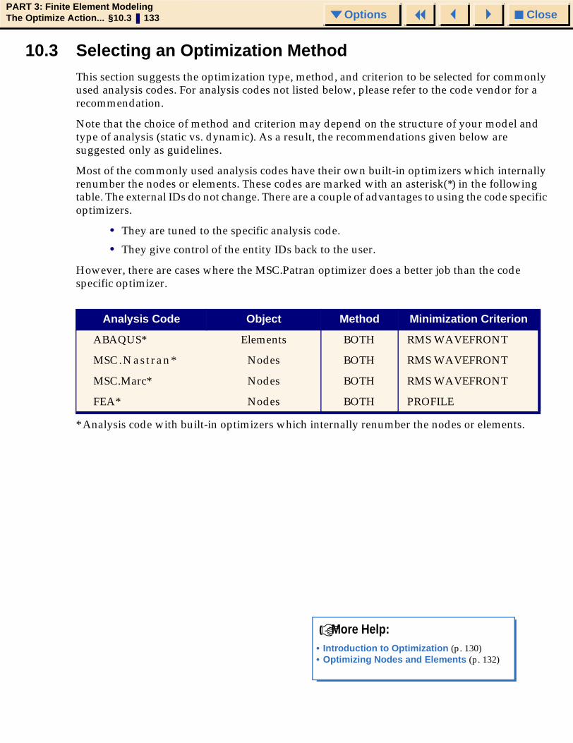
CloseOptionsPART 3: Finite Element ModelingThe Optimize Action... §10.3 133 Options
10.3 Selecting an Optimization MethodThis section suggests the optimization type, method, and criterion to be selected for commonly used analysis codes. For analysis codes not listed below, please refer to the code vendor for a recommendation.
Note that the choice of method and criterion may depend on the structure of your model and type of analysis (static vs. dynamic). As a result, the recommendations given below are suggested only as guidelines.
Most of the commonly used analysis codes have their own built-in optimizers which internally renumber the nodes or elements. These codes are marked with an asterisk(*) in the following table. The external IDs do not change. There are a couple of advantages to using the code specific optimizers.
• They are tuned to the specific analysis code.
• They give control of the entity IDs back to the user.
However, there are cases where the MSC.Patran optimizer does a better job than the code specific optimizer.
Analysis Code Object Method Minimization Criterion
ABAQUS*
* Analysis code with built-in optimizers which internally renumber the nodes or elements.
Elements BOTH RMS WAVEFRONT
MSC.Nastran* Nodes BOTH RMS WAVEFRONT
MSC.Marc* Nodes BOTH RMS WAVEFRONT
FEA* Nodes BOTH PROFILE
• Introduction to Optimization (p. 130)• Optimizing Nodes and Elements (p. 132)
☞ More Help:

CloseOptionsPART 3: Finite Element ModelingThe Optimize Action... §10.3 134 Options

CloseOptionsPART 3: Finite Element ModelingThe Verify Action § 135 Options
MSC.Patran Reference Manual, Part 3: Finite Element Modeling
CHAPTER
11 The Verify Action
■ Introduction to Verification
■ Verify Forms
■ Theory

CloseOptionsPART 3: Finite Element ModelingThe Verify Action §11.1 136 Options
11.1 Introduction to VerificationModel verification consists of a number of different tests which can be performed to check the validity of a finite element model. These tests include checks of element distortion, element duplication, model boundaries, nodal connectivity, and node ⁄element ID numbering.
In the case of distortion checking, MSC.Patran provides a series of automated tests to measure the “distortion” of elements from an “ideal” shape through measurable geometric properties of the element. The results of these tests are compared to user specified criteria and a determination is made whether the element is acceptable or not. The pass ⁄fail criteria is analysis code dependant and is updated automatically when the Analysis Preference is changed.
Verification tests are always performed on the current group of the active viewport except in the case of duplicate elements in which case the entire model is checked.
To get an overview when checking a specific element type, there is a test choice of All. When this is selected MSC.Patran will display a spreadsheet showing a summary of the total number of elements that exceed a threshold value for each of the distortion checks, and the actual test value and element ID number for the most extreme element.
Model Verification provides visual feedback of the selected test. Element distortion checks allow the selection of a threshold value using a slidebar. During the check, any element, which exceeds the threshold value, is highlighted and its value is listed in the Command Line. Upon completion of the check MSC.Patran will color code the elements based on the computed test value. Elements with a value higher than the threshold are colored with the highest spectrum color, all other values are assigned uniformly through the other spectrum levels. The current group will be rendered using the Element Fill style. Verification forms for Quad elements include an icon that allows a selection to split failed elements or simply highlight them.
Other checks, such as element duplication and connectivity, give options only to highlight any offending elements, or automatically correct the model.
Model boundaries may either be displayed as edge lines, showing unshared edges in the model, or as shaded faces, showing unshared surfaces.
All verification tests that involve color-coding, shading, or some other method of re-rendering the model have a Reset Graphics button on the form. Selecting this button will undo any rendering procedures performed by the most recent verification activity. The render style and spectrum display will be returned to the pre-test settings they had before the Apply button was selected. If you will be performing more than one type of verification test, it is recommended to choose Reset Graphics after each test is completed. Remember Reset Graphics resets to the settings prior to the current verification activity, not to those at the start of all verification.
All element specific verification forms have a Normalize button. By default, the normalize option will not be selected, and the slidebar will represent an actual value for the verification test threshold. If the normalize option may be selected, the slidebar will now represent a range of values from zero to one. The value of zero will represent the most reliable shape for this element type.
All element specific verification forms also have a Reset button. Selecting this button returns the slidebar and all toggles to the settings they had when the form was opened.
The information obtained from verification procedures can assist the engineer in deciding if the finite element model is satisfactory, or should be adjusted through remeshing or element modification.

CloseOptionsPART 3: Finite Element ModelingThe Verify Action §11.2 137 Options
11.2 Verify FormsWhen Verify is the selected Action the following options are available.
Object Test Description
Element Boundaries Plots the free edges or faces of finite elements.
Duplicates Checks elements for identical corner (or end) nodes.
Normals Compare adjacent shell normals.
Connectivity Check solid elements for proper connectivity using a volume calculation.
Geometry Fit Checks fit error distances between elements and their parent geometry.
Jacobian Ratio
Reports the maximum variation of the determinant of the Jacobian over each element.
Jacobian Zero
Reports the minimum determinant of the Jacobian for each element.
IDs Assigns color to the Finite Elements based on the Element ID number.
Tria All Tests tria elements for each of the tria verification tests. Reports the worst case for each test and the element at which it occurs.
Aspect Measures length to width ratio of tria elements.
Skew Tests tria elements for angular deviation using an edge bisector method.
Quad All Tests quad elements for each of the quad verification tests. Reports the worst case for each test and the element at which it occurs.
Aspect Measures length to width ratio of quad elements.
Warp Tests quad elements for deviation out of plane.
Skew Tests quad elements for angular deviation from a rectangular shape using an edge bisector method.
Taper Tests quad elements for geometric deviation from a rectangular shape.

CloseOptionsPART 3: Finite Element ModelingThe Verify Action §11.2 138 Options
Tet All Tests tet elements for each of the tet verification tests. Reports the worst case for each test and the element at which it occurs.
Aspect Compares ratio of height to square root of opposing face area of tet elements.
Edge Angle Calculates the maximum deviation angle between adjacent faces of tet elements.
Face Skew Tests each face of tet elements for angular deviation using an edge bisector method.
Collapse Tests tet elements for near zero volume.
Wedge All Tests wedge elements for each of the wedge verification tests. Reports the worst case for each test and the element at which it occurs.
Aspect Compares the maximum ratio of the height of the triangular sides to the distance between them for each wedge element.
Edge Angle Calculates the angular deviation between adjacent faces of wedge elements.
Face Skew Tests each face of wedge elements for angular deviation using an edge bisector method.
Face Warp Tests each quad face of wedge elements for deviation out of plane.
Twist Computes a twist angle between the two triangular faces of wedge elements.
Face Taper Tests each quad face of wedge elements for geometric deviation from a rectangular shape.
Hex All Tests hex elements for each of the hex verification tests. Reports the worst case for each test and the element at which it occurs.
Aspect Calculates the ratio of the maximum to minimum distance between opposing faces for each Hex element.
Edge Angle Calculates the angular deviation between adjacent faces of hex elements.
Face Skew Calculates the skew angle for each face of a hex element and reports the maximum.
Face Warp Calculates the deviation out of plane for each element face.
Twist Computes twist between the opposing faces of hex elements.
Face Taper Tests each Hex element for geometric deviation from a rectangular shape.
Object Test Description

CloseOptionsPART 3: Finite Element ModelingThe Verify Action §11.2 139 Options
Node IDs Computes contour lines based on the ID numbers of the Nodes.
Midnode Normal Offset
Calculates the ratio between the perpendicular offset of the midside node and the element edge length.
Tangent Offset
Measures the offset from the center of the element edge to the midside node. Calculates the ratio of this offset to the element edge length.
Superelement
Displays superelement’s boundaries with or without the boundary nodes.
Object Test Description

CloseOptionsPART 3: Finite Element ModelingThe Verify Action §11.2 140 Options
Verify - Element (Boundaries)
Finite Elements
Verify Action:
Element Object:
Boundaries Test:
Free Edges
Free Faces
Display Type
Reset Graphics
Apply
Plots the boundary as free edges, or optionally free faces, of all Posted elements in all viewports. A boundary is defined as any edge or face of a finite element which is not shared by at least one other element. Therefore, this test will display, in addition to interior and exterior edges/faces of the group, any interior “cracks”. Cracks will appear along geometric boundaries prior to equivalencing.
Returns your graphic display to the way it was when the form was opened. This will either change from Flat Shaded (for free faces) or Boundary Line (for free edges) back to the original Render Style. If you were originally using entity type display mode, this will again become the default. Exiting this form will reset graphics.
Selecting Free Edges displays any unshared edges that define the boundary of your current group in yellow.
Selecting Free Faces displays any unshared faces in your current group in a yellow Flat Shaded render style.
Important: If you are in entity type display mode when you start boundary verification, MSC.Patran will temporarily enter group display mode to display the group boundaries.
◆
◆◆

CloseOptionsPART 3: Finite Element ModelingThe Verify Action §11.2 141 Options
Verify - Element (Duplicates)Elements in the entire model are checked for identical corner (or end) nodes.
Finite Elements
Verify Action:
Element Object:
Duplicates Test:
Display Only
Delete Higher ID Delete Lower ID
Test Control
Reset Graphics
Apply
Returns your graphic display back to the way it was when the form was opened.This will unhighlight duplicate elements. Exiting this form will also reset graphics.
MSC.Patran gives the option to highlight any duplicate elements found, or, if you select the icon, you may choose to have MSC.Patran automatically eliminate any duplicates found. When delete duplicates is selected you may choose which element ID of the two to remove from the database.
◆
◆◆

CloseOptionsPART 3: Finite Element ModelingThe Verify Action §11.2 142 Options
Verify - Element (Normals)Figure 11-1
Finite Elements
Verify Action:
Element Object:
Normals Test:
Color Code Elements Draw Normal Vectors
Display Control
Display Only
Test Control
Reset Graphics
Apply
There are two options for displaying the element normal information:
1. The elements may be color-coded. Elements will initially be colored white, any element whose normal is reversed will be highlighted in red.Note: Be sure to equivalence your model before color coding. This is necessary because the color-coding algorithm only compares elements with shared edges.
2. Or MSC.Patran may draw the normal vectors and plot arrows pointing from the element centroids in the element normal direction.
Normal directions are processed for each shell element in the current group in the active viewport.
There are two available options for controlling what MSC.Patran does with the element normal information:
1. The default choice is Display Only which tells MSC.Patran the only action you want it to take is to graphically display the normal information.
2. Or you may select the Display Only icon to change the test control to Reverse Elements. This allows you to specify (or select) a Guiding Element to which all other element normals in your current group will be matched.
◆
◆◆
Fringe Attributes
Returns your graphic display to the way it was when the form was opened. This will usually change from Element Fill back to the original Render Style, or will remove all those little vectors from the viewport. Exiting this form will also reset graphics.
See Fringe Attributes (p. 223) in the MSC.Patran Reference Manual, Part 6: Results Postprocessing

CloseOptionsPART 3: Finite Element ModelingThe Verify Action §11.2 143 Options
Verify - Element (Connectivity)All solid elements in the current group in the active viewport are checked for proper connectivity using a volume calculation.
Finite Elements
Verify Action:
Element Object:
Connectivity Test:
Highlight Only
Apply
Elements found to have negative volume will be color coded for identification purposes when the highlight only icon is selected. Otherwise, the offending elements will be automatically reversed when the reverse icon is selected.
2
1
• MSC.Patran’s Element Library (p. 320) ☞ More Help:

CloseOptionsPART 3: Finite Element ModelingThe Verify Action §11.2 144 Options
Verify - Element (Geometry Fit)All elements in the current group in the active viewport are checked for maximum distance between the element and the parent geometry.
Enter the maximum acceptable distance between an element and its parent geometry.
Returns your graphic display back to the way it was when the form was opened. This will usually change from Element Fill back to the original Render Style and remove the spectrum display from your viewport.
Finite Elements
Verify Action:
Element Object:
Geometry FitTest:
Element Plot Options
Color Code Elements
Plot Failed Elements Only
Threshold h Value =0.001Toggle to control element plot options. You can either color code the elements and/or plot only the elements in the current group that were tested and failed.
Note: Linear elements such as Bar/2, Quad/4, and Hex/8 are evaluated at one point per bar or element face. Quadratic elements such as Bar/3, Quad/8, and Hex/20 are evaluated at two points per bar or four points per element face. Cubic elements such as Bar/4, Quad/12, and Hex/32 are evaluated at three points per bar or nine points per element face.
Reset Graphics
Apply
Fringe Attributes
See Fringe Attributes (p. 223) in the MSC.Patran Reference Manual, Part 6: Results Postprocessing

CloseOptionsPART 3: Finite Element ModelingThe Verify Action §11.2 145 Options
Verify - Element (Jacobian Ratio)The ratio of the maximum determinant of the Jacobian to the minimum determinant of the Jacobian is calculated for each element in the current group in the active viewport. This element shape test can be used to identify elements with interior corner angles far from 90 degrees or high order elements with misplaced midside nodes. A ratio close or equal to 1.0 is desired.
Finite Elements
Verify Action:
Element Object:
Jacobian Ratio Test:
Returns your graphic display to the way it was when you entered the form. This will usually change from Element Fill back to the original Render Style, and remove the spectrum display from your viewport.
Note: The minimum and maximum ratios and the associated elements are echoed in the command line. Elements in the current group are color-coded according to the value of the Jacobian ratio and will be plotted in the Element Fill render style.
J1
J2
J
J2
1
Reset Graphics
Apply
Fringe Attributes
See Fringe Attributes (p. 223) in the MSC.Patran Reference Manual, Part 6: Results Postprocessing

CloseOptionsPART 3: Finite Element ModelingThe Verify Action §11.2 146 Options
Verify - Element (Jacobian Zero)The determinant of the Jacobian (J) is calculated at all integration points for each element in the current group in the active viewport. The minimum value for each element is determined. This element shape test can be used to identify incorrectly shaped elements. A well-formed element will have J positive at each Gauss point and not greatly different from the value of J at other Gauss points. J approaches zero as an element vertex angle approaches 180 degrees.
Finite Elements
Verify Action:
Element Object:
Jacobian Zero Test:
Returns your graphic display to the way it was when the form was opened. This will usually change from Element Fill back to the original Render Style, and remove the spectrum display from your viewport.
Note: The minimum and maximum value and the associated elements are echoed in the command line. Elements in the current group are color-coded according to the value of the determinant of the Jacobian and will be plotted in the Element Fill render style.
J1
J2
Min ( ,J1 J2 )
Reset Graphics
Apply
Fringe Attributes
See Fringe Attributes (p. 223) in the MSC.Patran Reference Manual, Part 6: Results Postprocessing
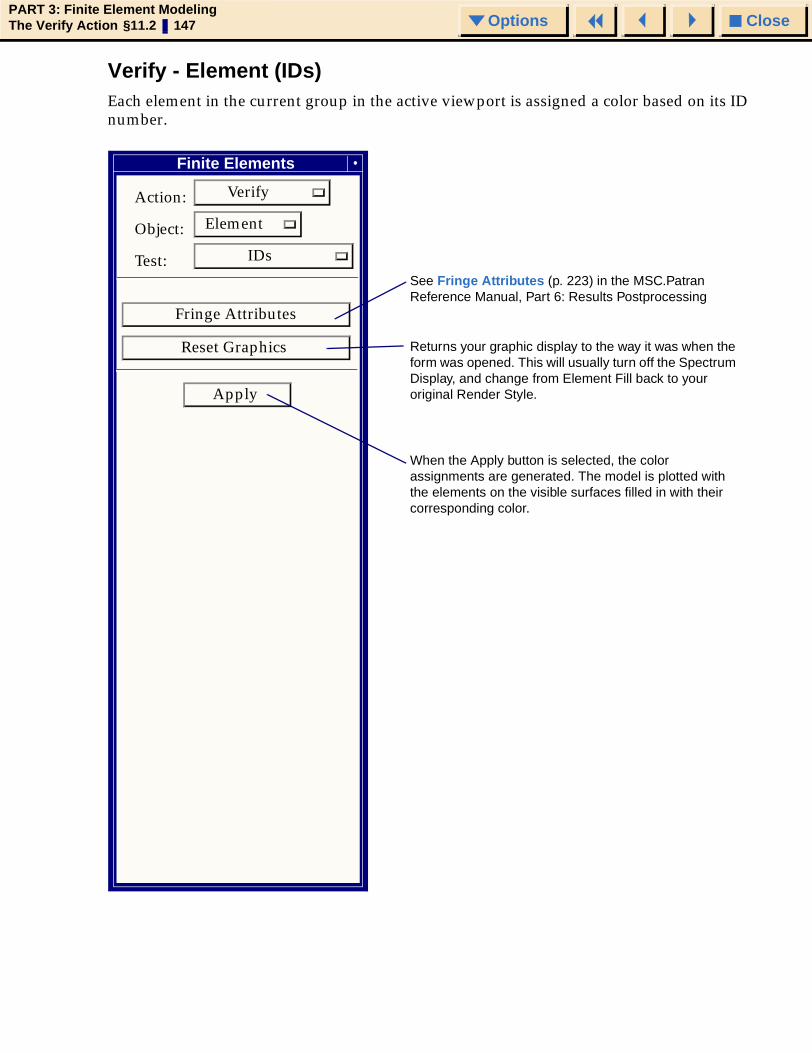
CloseOptionsPART 3: Finite Element ModelingThe Verify Action §11.2 147 Options
Verify - Element (IDs)Each element in the current group in the active viewport is assigned a color based on its ID number.
Finite Elements
Verify Action:
Element Object:
IDs Test:
Returns your graphic display to the way it was when the form was opened. This will usually turn off the Spectrum Display, and change from Element Fill back to your original Render Style.
When the Apply button is selected, the color assignments are generated. The model is plotted with the elements on the visible surfaces filled in with their corresponding color.
Reset Graphics
Apply
Fringe Attributes
See Fringe Attributes (p. 223) in the MSC.Patran Reference Manual, Part 6: Results Postprocessing

CloseOptionsPART 3: Finite Element ModelingThe Verify Action §11.2 148 Options
Verify - Tria (All)Each tria element in the current group is tested for each of the tria verification tests.
Finite Elements
Verify Action:
Tria Object:
All Test:
Normalize
Analysis Code: MSC.Nastran
Aspect Ratio: 5.
Skew Angle: 30.
Normal Offset: 0.15
Tangent Offset: 0.15
Reliability Threshold
Apply When the Apply button is selected, a spreadsheet will be displayed showing the worst case value for each test and the element at which it occurs.
Write to Report

CloseOptionsPART 3: Finite Element ModelingThe Verify Action §11.2 149 Options
Verify - Tria (All) Spreadsheet
Tria Verification Summary
Test Number Failed Worst Case At Element
Aspect
Skew
Normal Offset 1
2
2 max=4.185907
max=61.91709 1
max=1.192093E-06 212
83
359
This column lists the Verification test. All tests listed on the application form will be performed. Use the scroll bar to view additional tests.
The last two columns list the maximum (or minimum, if applicable) value of the test and the element at which this worst case occurs.
This column lists the number of elements in the current group that exceeded the reliability threshold shown on the application form.

CloseOptionsPART 3: Finite Element ModelingThe Verify Action §11.2 150 Options
Verify - Tria (Aspect)All of the tria elements in the current group of the active viewport are tested for length to width ratio.
When the Normalize button is selected, the computed aspect ratio is inverted and subtracted from 1. When the Normalize button is turned OFF, the slidebar represents the computed Aspect Ratio. Move the slidebar to indicate the maximum acceptable value for your analysis type and code.
Returns your graphic display to the way it was when the form was opened. This will usually turn off the Spectrum Display, and change from Element Fill back to your original Render Style.
• Aspect Ratio (p. 187)
☞ More Help:
Action: Verify
Object: Object: Object: Object: Tria
Test: Aspect
Reliability Threshold
Normalize
Analysis Code: MSC.Nastran
20.1.
Element Plot Options
Color Code Elements
Plot Failed Elements Only
h1
h23 h2
2 h1
√
1.00
Finite Elements
Toggle to control element plot options. You can either color code the elements and/or plot only the elements in the current group, which were tested and failed.
Reset Graphics
Apply Reset
Fringe Attributes
See Fringe Attributes (p. 223) in the MSC.Patran Reference Manual, Part 6: Results Postprocessing
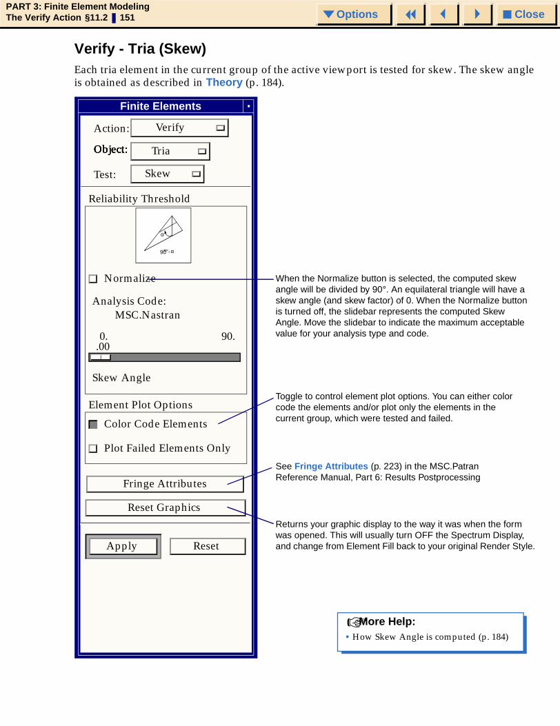
CloseOptionsPART 3: Finite Element ModelingThe Verify Action §11.2 151 Options
Verify - Tria (Skew)Each tria element in the current group of the active viewport is tested for skew. The skew angle is obtained as described in Theory (p. 184).
Returns your graphic display to the way it was when the form was opened. This will usually turn OFF the Spectrum Display, and change from Element Fill back to your original Render Style.
When the Normalize button is selected, the computed skew angle will be divided by 90°. An equilateral triangle will have a skew angle (and skew factor) of 0. When the Normalize button is turned off, the slidebar represents the computed Skew Angle. Move the slidebar to indicate the maximum acceptable value for your analysis type and code.
• How Skew Angle is computed (p. 184) ☞ More Help:
Action: Verify
Object: Object: Object: Object: Tria
Test: Skew
Reliability Threshold
Normalize
Analysis Code: MSC.Nastran
90. 0.
Element Plot Options
Color Code Elements
Plot Failed Elements Only
α
90× α°-
.00
Skew Angle
Finite Elements
Toggle to control element plot options. You can either color code the elements and/or plot only the elements in the current group, which were tested and failed.
Reset Graphics
Apply Reset
Fringe Attributes
See Fringe Attributes (p. 223) in the MSC.Patran Reference Manual, Part 6: Results Postprocessing

CloseOptionsPART 3: Finite Element ModelingThe Verify Action §11.2 152 Options
Verify - Quad (All)Each quad element in the current group of the active viewport is tested for each of the quad verification tests.
Finite Elements
Verify Action:
Quad Object:
All Test:
Normalize
Analysis Code: MSC.Nastran
Aspect Ratio: 5.0
Warp Angle: 7.0
Skew Angle: 30.
Taper: 0.8
Normal Offset: 0.15
Tangent Offset: 0.15
Reliability Threshold
Apply
When the Apply button is selected a spreadsheet will be displayed showing the worst case value for each test and the element at which it occurs.
• Spreadsheet Information (p. 153) • Test Definitions (p. 184)
☞ More Help:

CloseOptionsPART 3: Finite Element ModelingThe Verify Action §11.2 153 Options
Verify - Quad (All) Spreadsheet
Quad Verification Summary
Test Number Failed Worst Case At Element
Aspect
Warp
Skew 1
0
14 max=3.2461078
max=0.
max=51.957664 260
0
260
This column lists the Verification test. All tests listed on the application form will be performed. Use the scroll bar to view additional tests.
The last two columns list the maximum (or minimum, if applicable) value of the test and the element at which this worst case occurs.
This column lists the number of elements in the current group that exceeded the reliability threshold shown on the application form.
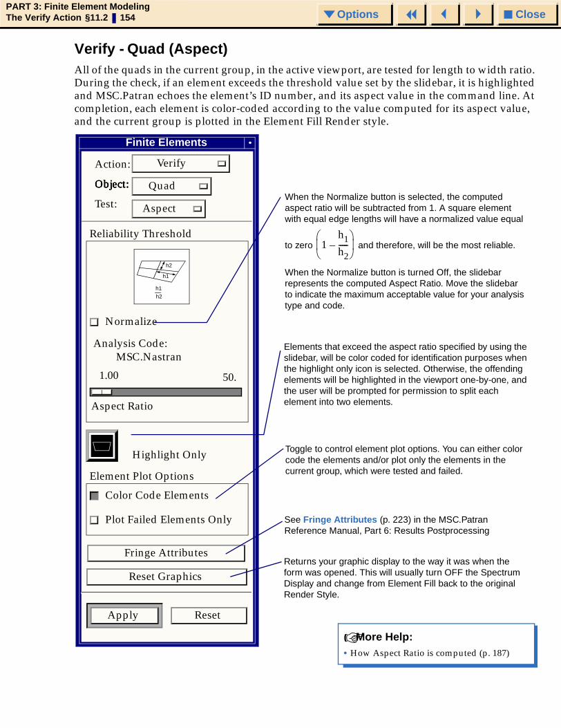
CloseOptionsPART 3: Finite Element ModelingThe Verify Action §11.2 154 Options
Verify - Quad (Aspect)All of the quads in the current group, in the active viewport, are tested for length to width ratio. During the check, if an element exceeds the threshold value set by the slidebar, it is highlighted and MSC.Patran echoes the element’s ID number, and its aspect value in the command line. At completion, each element is color-coded according to the value computed for its aspect value, and the current group is plotted in the Element Fill Render style.
Elements that exceed the aspect ratio specified by using the slidebar, will be color coded for identification purposes when the highlight only icon is selected. Otherwise, the offending elements will be highlighted in the viewport one-by-one, and the user will be prompted for permission to split each element into two elements.
Returns your graphic display to the way it was when the form was opened. This will usually turn OFF the Spectrum Display and change from Element Fill back to the original Render Style.
• How Aspect Ratio is computed (p. 187) ☞ More Help:
When the Normalize button is selected, the computed aspect ratio will be subtracted from 1. A square element with equal edge lengths will have a normalized value equal
to zero and therefore, will be the most reliable.
When the Normalize button is turned Off, the slidebar represents the computed Aspect Ratio. Move the slidebar to indicate the maximum acceptable value for your analysis type and code.
1h1h2-----–
Action: Verify
Object: Object: Object: Object: Quad
Test: Aspect
Reliability Threshold
Normalize
Analysis Code: MSC.Nastran
50.
Highlight Only
Element Plot Options
Color Code Elements
Plot Failed Elements Only
Finite Elements
h2
h1
h2
h1
Aspect Ratio
1.00
Toggle to control element plot options. You can either color code the elements and/or plot only the elements in the current group, which were tested and failed.
Reset Graphics
Apply Reset
Fringe Attributes
See Fringe Attributes (p. 223) in the MSC.Patran Reference Manual, Part 6: Results Postprocessing

CloseOptionsPART 3: Finite Element ModelingThe Verify Action §11.2 155 Options
Verify - Quad (Warp)Each quad element in the current group of the active viewport is tested for warp. The warp angle is obtained as described in Theory (p. 184). During the check, MSC.Patran highlights any element exceeding the threshold value set by the slidebar, and echoes the element’s ID number and its warp value in the command line. At completion, each element is color-coded according to the value computed for its warp value and the current group is plotted in the Element Fill Render style.
When the Normalize button is selected, the computed warp angle will be divided by 15°. A “perfect” element will have no out-of-plane component and will therefore be the most reliable. When the Normalize button is turned off, the slidebar represents the computed Warp Angle. Move the slidebar to indicate the maximum acceptable value for your analysis type and code.
Elements that exceed the warp angle specified by using the slidebar, will be color coded for identification purposes when the highlight only icon is selected. Otherwise, the offending elements will be highlighted in the viewport one-by-one, and the user will be prompted for permission to split each element into two tria elements.
Returns your graphic display to the way it was when the form was opened. This will usually turn OFF the Spectrum Display and change from Element Fill back to your original Render Style.
• How Warp Angle is computed (p. 191) ☞ More Help:
Finite Elements
Action: Verify
Object: Object: Quad
Test: Warp
Reliability Threshold
Normalize
Analysis Code: MSC.Nastran
90.
Highlight Only
Element Plot Options
Color Code Elements
Plot Failed Elements Only
θ
.00
Warp Angle
Toggle to control element plot options. You can either color code the elements and/or plot only the elements in the current group, which were tested and failed.
0.
Reset Graphics
Apply Reset
Fringe Attributes
See Fringe Attributes (p. 223) in the MSC.Patran Reference Manual, Part 6: Results Postprocessing

CloseOptionsPART 3: Finite Element ModelingThe Verify Action §11.2 156 Options
Verify - Quad (Skew)Each quad element in the current group in the active viewport is tested for skew. The skew angle is obtained as described in Theory (p. 184). Prior to testing for skew, each element is checked for convexity. If any element fails the convexity, test a warning message will be issued. Processing will continue on to the next element.
When the Normalize button is selected the computed skew angle will be divided by 90°. A “perfect” element with corner angles of 90° will have a normalized value equal to zero
and will therefore be the most reliable. When the
Normalize button is turned OFF, the slidebar represents the computed Skew Angle. Move the slidebar to indicate the maximum acceptable value for your analysis type and code.
90° α–90°------------------
Returns your graphic display to the way it was when the form was opened. This will usually turn OFF the Spectrum Display and change from Element Fill back to your original Render Style.
• How Skew Angle is computed (p. 184) ☞ More Help:
Elements that exceed the skew angle specified by using the slidebar, will be color coded for identification purposes when the highlight only icon is selected. Otherwise, the offending elements will be highlighted in the viewport one-by-one, and the user will be prompted for permission to split each element into two tria elements.
Finite Elements
Action: Verify
Object: Object: Quad
Test: Skew
Reliability Threshold
Normalize
Analysis Code: MSC.Nastran
90. 0.
Highlight Only
Element Plot Options
Color Code Elements
Plot Failed Elements Only
.00
Skew Angle
α
90× α°-
Toggle to control element plot options. You can either color code the elements and/or plot only the elements in the current group, which were tested and failed.
Reset Graphics
Apply Reset
Fringe Attributes
See Fringe Attributes (p. 223) in the MSC.Patran Reference Manual, Part 6: Results Postprocessing.

CloseOptionsPART 3: Finite Element ModelingThe Verify Action §11.2 157 Options
Verify - Quad (Taper)Each quad element in the current group in the active viewport is tested for taper. The taper ratio is obtained as described in Theory (p. 184).
When the Normalize button is selected, the computed Taper ratio will be subtracted from 1. A “perfect” element will have all 4 triangular subareas (a) equal; therefore, 4*a⁄total area will equal 1 and the normalized equation will yield a taper factor of 0. When the Normalize button is turned OFF, the slidebar represents the computed Taper Ratio. Move the slidebar to indicate the maximum acceptable value for your analysis type and code.
• How Taper is computed (p. 192) ☞ More Help:
Elements that exceed the Taper ratio specified by using the slidebar, will be color coded for identification purposes when the highlight only icon is selected. Otherwise, the offending elements will be highlighted in the viewport one-by-one, and the user will be prompted for permission to split each element into two quad elements.
Returns your graphic display to the way it was when the form was opened. This will usually turn OFF the Spectrum Display and change from Element Fill back to your original Render Style.
Finite Elements
Action: Verify
Object: Object: Quad
Test: Taper
Reliability Threshold
Normalize
Analysis Code: MSC.Nastran
90.0.
Highlight Only
Element Plot Options
Color Code Elements
Plot Failed Elements Only
.00
Taper Angle
4 aA
a
Toggle to control element plot options. You can either color code the elements and/or plot only the elements in the current group, which were tested and failed.
Reset Graphics
Apply Reset
Fringe Attributes
See Fringe Attributes (p. 223) in the MSC.Patran Reference Manual, Part 6: Results Postprocessing.

CloseOptionsPART 3: Finite Element ModelingThe Verify Action §11.2 158 Options
Verify - Tet (All)Each Tetrahedral element in the current group is tested for each of the Tet verification tests.
Finite Elements
Verify Action:
Tet Object:
All Test:
Normalize
Analysis Code: MSC.Nastran
Aspect Ratio: 5.0
Edge Angle: 30.
Face Skew: 30.
Collapse: 0.15
Normal Offset: 0.15
Tangent Offset: 0.15
Reliability Threshold
Apply When the Apply button is selected, a spreadsheet will be displayed showing the worst case value for each test and the element at which it occurs.
• Spreadsheet Information (p. 159) • Test Definition (p. 184)
☞ More Help:

CloseOptionsPART 3: Finite Element ModelingThe Verify Action §11.2 159 Options
Verify - Tet (All) Spreadsheet
Tet Verification Summary
Test Number Failed Worst Case At Element
Aspect
Edge Angle
Face Skew 1
40
14 Max=4.0778556
Max=55.064632
Max=67.38166 16
135
11
This column lists the Verification test. All tests listed on the application form will be performed. Use the scroll bar to view additional tests.
The last two columns list the maximum (or minimum, if applicable) value of the test and the element at which this worst case occurs.
This column lists the number of elements in the current group that exceeded the reliability threshold shown on the application form.

CloseOptionsPART 3: Finite Element ModelingThe Verify Action §11.2 160 Options
Verify - Tet (Aspect)All of the Tets in the current group are tested for the ratio of height to square root of opposing face area. During the check, MSC.Patran highlights any element exceeding the threshold value set by the slidebar, and echoes the element’s ID number and its aspect ratio in the command line. At completion, each element is color-coded according to the value computed for its aspect ratio and the current group is plotted in the Element Fill Render style.
When the Normalize button is selected, the computed aspect ratio will be subtracted from 1. When the Normalize button is turned OFF, the slidebar represents the computed Aspect Ratio. Move the slidebar to indicate the maximum acceptable value for your analysis type and code.
• How Aspect Ratio is computed (p. 188)
☞ More Help:
Returns your graphic display to the way it was when the form was opened. This will usually turn OFF the Spectrum Display and change from Element Fill back to your original Render Style.
Finite Elements
Action: Verify
Object: Object: Tet
Test: Aspect
Reliability Threshold
Normalize
Analysis Code: MSC.Nastran
20. 1.
Element Plot Options
Color Code Elements
Plot Failed Elements Only
1.00
Aspect Ratio
hi
Ai
Max (c . hi⁄√Ai)cζ = .805927
Toggle to control element plot options. You can either color code the elements and/or plot only the elements in the current group, which were tested and failed.
Reset Graphics
Apply Reset
Fringe Attributes
See Fringe Attributes (p. 223) in the MSC.Patran Reference Manual, Part 6: Results Postprocessing.

CloseOptionsPART 3: Finite Element ModelingThe Verify Action §11.2 161 Options
Verify - Tet (Edge Angle)
When the Normalize button is selected, the computed edge angle will be divided by 110°. When the Normalize button is turned OFF, the slidebar represents the computed Edge Angle. Move the slidebar to indicate the maximum acceptable value for your analysis type and code.
• How Edge Angle is computed (p. 193)
☞ More Help:
All of the tetrahedral elements in the current group of the active viewport are tested for the maximum angle between adjacent faces. An edge angle is the absolute value of the angle between the two faces meeting at an edge subtracted from 70.529°. During the check, MSC.Patran highlights any element exceeding the threshold value set by the slidebar, and echoes the element’s ID number and its edge angle in the command line. At completion, each element is color-coded according to the edge angle and the current group is plotted in the Element Fill Render style.
Returns your graphic display to the way it was when the form was opened. This will usually turn off the Spectrum Display and change from Element Fill back to your original Render Style.
Finite Elements
Action: Verify
Object: Object: Tet
Test: Edge Angle
Reliability Threshold
Normalize
Analysis Code: MSC.Nastran
110. 0.
Element Plot Options
Color Code Elements
Plot Failed Elements Only
1.00
Edge Angle
- 70.53
α
α °
Toggle to control element plot options. You can either color code the elements and/or plot only the elements in the current group, which were tested and failed.
Reset Graphics
Apply Reset
Fringe AttributesSee Fringe Attributes (p. 223) in the MSC.Patran Reference Manual, Part 6: Results Postprocessing.

CloseOptionsPART 3: Finite Element ModelingThe Verify Action §11.2 162 Options
Verify - Tet (Face Skew)Each face of each tetrahedral element in the current group is tested for skew as if it were a Tria element. The skew angle is obtained as described in Theory (p. 184). During the check, MSC.Patran highlights any element exceeding the threshold value set by the slidebar, and echoes the element’s ID number and its maximum skew angle in the command line. At completion, each element is color-coded according to the value computed for its skew angle and the current group is plotted in the Element Fill Render style.
When the Normalize button is selected, the computed skew angle will be divided by 90°. An equilateral triangle will have a skew angle of 0. When the Normalize button is turned OFF, the slidebar represents the computed skew angle. Move the slidebar to indicate the maximum acceptable value for your analysis type and code.
Returns your graphic display to the way it was when the form was opened. This will usually turn off the Spectrum Display and change from Element Fill back to your original Render Style.
Finite Elements
Action: Verify
Object: Object: Tet
Test: Face Skew
Reliability Threshold
Normalize
Analysis Code: MSC.Nastran
90. 0.
Element Plot Options
Color Code Elements
Plot Failed Elements Only
.00
Face Skew Angle
α
90× α°-
Toggle to control element plot options. You can either color code the elements and/or plot only the elements in the current group, which were tested and failed.
Reset Graphics
Apply Reset
Fringe Attributes See Fringe Attributes (p. 223) in the MSC.Patran Reference Manual, Part 6: Results Postprocessing.

CloseOptionsPART 3: Finite Element ModelingThe Verify Action §11.2 163 Options
Verify - Tet (Collapse)All of the tetrahedral elements in the current group are tested for volume. The collapse value is obtained as described in Theory (p. 184). During the check, MSC.Patran highlights any element exceeding the threshold value set by the slidebar, and echoes the element’s ID number and its collapse value in the command line. At completion, each element is color-coded according to the collapse value and the current group is plotted in the Element Fill Render style.
When the Normalize button is selected, the computed collapse ratio will be subtracted from 1. For an equilateral tet, the collapse value will equal 1, therefore,
will equal zero, and will be the
most reliable element. When the Normalize button is turned Off, the slidebar represents the computed collapse value. Move the slidebar to indicate the maximum acceptable value for your analysis type and code.
1 Min hi Ai( )⁄( )–
• How Collapse is computed (p. 195)
☞ More Help:
Returns your graphic display to the way it was when the form was opened. This will usually turn off the Spectrum Display and change from Element Fill back to your original Render Style.
Finite Elements
Action: Verify
Object: Object: Tet
Test: Collapse
Reliability Threshold
Normalize
Analysis Code: MSC.Nastran
10. 0.
Element Plot Options
Color Code Elements
Plot Failed Elements Only
.00
Collapse Ratio
hi
Ai
Min (hi⁄√ Ai)
Toggle to control element plot options. You can either color code the elements and/or plot only the elements in the current group, which were tested and failed.
Reset Graphics
Apply Reset
Fringe Attributes
See Fringe Attributes (p. 223) in the MSC.Patran Reference Manual, Part 6: Results Postprocessing.

CloseOptionsPART 3: Finite Element ModelingThe Verify Action §11.2 164 Options
Verify - Wedge (All) Each wedge element in the current group of the active viewport is tested for each of the wedge verification tests.
Finite Elements
Verify Action:
Wedge Object:
All Test:
Normalize
Analysis Code: MSC.Nastran
Aspect Ratio: 5.0
Edge Angle: 30.
Face Skew: 30.
Face Warp: 7.0
Twist:45.0
Face Taper: 0.8
Normal Offset: 0.15
Tangent Offset: 0.15
Reliability Threshold
Apply
When the Apply button is selected, a spreadsheet will be displayed showing the worst case value for each test and the element at which it occurs.
• Spreadsheet Information (p. 165) • Test Definitions (p. 184)
☞ More Help:

CloseOptionsPART 3: Finite Element ModelingThe Verify Action §11.2 165 Options
Verify - Wedge (All) Spreadsheet
Wedge Verification Summary
Test Number Failed Worst Case At Element
Aspect
Edge Angle
Face Skew 1
40
14 Max=4.0778556
Max=55.064632
Max=67.38166 16
135
11
This column lists the Verification test. All tests listed on the application form will be performed. Use the scroll bar to view additional tests.
The last two columns list the maximum (or minimum, if applicable) value of the test and the element at which this worst case occurs.
This column lists the number of elements in the current group that exceeded the reliability threshold shown on the application form.
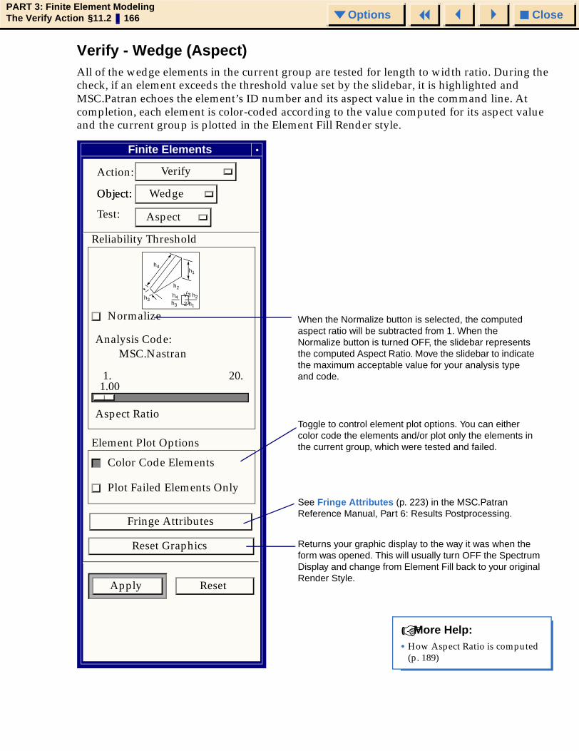
CloseOptionsPART 3: Finite Element ModelingThe Verify Action §11.2 166 Options
Verify - Wedge (Aspect)All of the wedge elements in the current group are tested for length to width ratio. During the check, if an element exceeds the threshold value set by the slidebar, it is highlighted and MSC.Patran echoes the element’s ID number and its aspect value in the command line. At completion, each element is color-coded according to the value computed for its aspect value and the current group is plotted in the Element Fill Render style.
When the Normalize button is selected, the computed aspect ratio will be subtracted from 1. When the Normalize button is turned OFF, the slidebar represents the computed Aspect Ratio. Move the slidebar to indicate the maximum acceptable value for your analysis type and code.
• How Aspect Ratio is computed (p. 189)
☞ More Help:
Returns your graphic display to the way it was when the form was opened. This will usually turn OFF the Spectrum Display and change from Element Fill back to your original Render Style.
Finite Elements
Action: Verify
Object: Object: Wedge
Test: Aspect
Reliability Threshold
Normalize
Analysis Code: MSC.Nastran
20. 1.
Element Plot Options
Color Code Elements
Plot Failed Elements Only
1.00
Aspect Ratio
h1
3 h2
2 h1
√h3
h4 ⋅
h4
h3
h2
Toggle to control element plot options. You can either color code the elements and/or plot only the elements in the current group, which were tested and failed.
Reset Graphics
Apply Reset
Fringe Attributes
See Fringe Attributes (p. 223) in the MSC.Patran Reference Manual, Part 6: Results Postprocessing.

CloseOptionsPART 3: Finite Element ModelingThe Verify Action §11.2 167 Options
Verify - Wedge (Edge Angle)The maximum edge angle is calculated for each wedge element in the current group of the active viewport. Edge angle is obtained as described in Theory (p. 184). During the check, MSC.Patran highlights any element exceeding the threshold value set by the slidebar, and echoes the element’s ID number and its maximum edge angle in the command line. At completion, each element is color-coded according to the value computed for its edge angle and the current group is plotted in the Element Fill Render style.
When the Normalize button is selected, the computed Edge Angle will be divided by 110°. When the Normalize button is turned OFF, the slidebar represents the computed Edge Angle. Move the slidebar to indicate the maximum acceptable value for your analysis type and code.
• How Edge Angle is computed (p. 194)
☞ More Help:
Returns your graphic display to the way it was when the form was opened. This will usually turn OFF the Spectrum Display and change from Element Fill back to your original Render Style.
Finite Elements
Action: Verify
Object: Object: Wedge
Test: Edge Angle
Reliability Threshold
Normalize
Analysis Code: MSC.Nastran
110. 0.
Element Plot Options
Color Code Elements
Plot Failed Elements Only
.00
Edge Angle
× α )× °-90Max (60°-θ,
α
θ
Toggle to control element plot options. You can either color code the elements and/or plot only the elements in the current group, which were tested and failed.
Reset Graphics
Apply Reset
Fringe Attributes
See Fringe Attributes (p. 223) in the MSC.Patran Reference Manual, Part 6: Results Postprocessing.

CloseOptionsPART 3: Finite Element ModelingThe Verify Action §11.2 168 Options
Verify - Wedge (Face Skew)Each face of each wedge element in the current group is tested for skew as if it were a quad or tria element. The skew angle is obtained as described in Theory (p. 184). During the check, MSC.Patran highlights any element exceeding the threshold value set by the slidebar, and echoes the element’s ID number and its maximum skew angle in the command line. At completion, each element is color-coded according to the value computed for its skew angle and the current group is plotted in the Element Fill Render style.
When the Normalize button is selected, the computed skew angle will be divided by 15°. When the Normalize button is turned OFF, the slidebar represents the computed Skew Angle. Move the slidebar to indicate the maximum acceptable value for your analysis type and code.
Returns your graphic display to the way it was when the form was opened. This will usually turn OFF the Spectrum Display and change from Element Fill back to your original Render Style.
Toggle to control element plot options. You can either color code the elements and/or plot only the elements in the current group, which were tested and failed.
Finite Elements
Action: Verify
Object: Object: Wedge
Test: Face Skew
Reliability Threshold
Normalize
Analysis Code: MSC.Nastran
90. 0.
Element Plot Options
Color Code Elements
Plot Failed Elements Only
.00
Face Skew Angle
×
α
90× α°-
1
α 2Min ( i )
Reset Graphics
Apply Reset
Fringe Attributes See Fringe Attributes (p. 223) in the MSC.Patran Reference Manual, Part 6: Results Postprocessing.
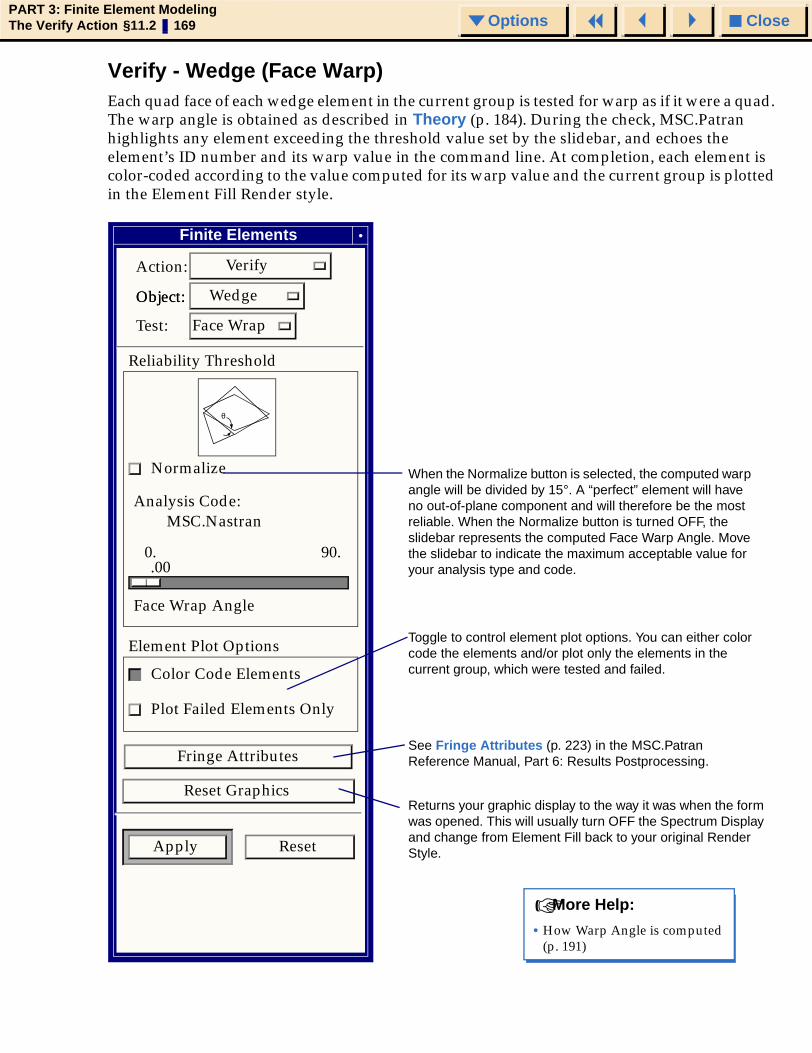
CloseOptionsPART 3: Finite Element ModelingThe Verify Action §11.2 169 Options
Verify - Wedge (Face Warp)Each quad face of each wedge element in the current group is tested for warp as if it were a quad. The warp angle is obtained as described in Theory (p. 184). During the check, MSC.Patran highlights any element exceeding the threshold value set by the slidebar, and echoes the element’s ID number and its warp value in the command line. At completion, each element is color-coded according to the value computed for its warp value and the current group is plotted in the Element Fill Render style.
When the Normalize button is selected, the computed warp angle will be divided by 15°. A “perfect” element will have no out-of-plane component and will therefore be the most reliable. When the Normalize button is turned OFF, the slidebar represents the computed Face Warp Angle. Move the slidebar to indicate the maximum acceptable value for your analysis type and code.
• How Warp Angle is computed (p. 191)
☞ More Help:
Returns your graphic display to the way it was when the form was opened. This will usually turn OFF the Spectrum Display and change from Element Fill back to your original Render Style.
Finite Elements
Action: Verify
Object: Object: Wedge
Test: Face Wrap
Reliability Threshold
Normalize
Analysis Code: MSC.Nastran
90. 0.
Element Plot Options
Color Code Elements
Plot Failed Elements Only
.00
Face Wrap Angle
θ
Toggle to control element plot options. You can either color code the elements and/or plot only the elements in the current group, which were tested and failed.
Reset Graphics
Apply Reset
Fringe AttributesSee Fringe Attributes (p. 223) in the MSC.Patran Reference Manual, Part 6: Results Postprocessing.

CloseOptionsPART 3: Finite Element ModelingThe Verify Action §11.2 170 Options
Verify - Wedge (Twist)Each wedge element in the current group is tested for a twist angle computed between its two triangular faces. Twist is obtained as described in Theory (p. 184). During the check, MSC.Patran highlights any element exceeding the threshold value set by the slidebar, and echoes the element’s ID number and its maximum twist in the command line. At completion, each element is color-coded according to the value computed for its twist and the current group is plotted in the Element Fill Render style.
When the Normalize button is selected, the computed twist angle will be divided by 60°. When the Normalize button is turned OFF, the slidebar represents the computed Twist Angle. Move the slidebar to indicate the maximum acceptable value for your analysis type and code.
• How Twist is computed (p. 196)☞ More Help:
Returns your graphic display to the way it was when the form was opened. This will usually turn OFF the Spectrum Display and change from Element Fill back to your original Render Style.
Finite Elements
Action: Verify
Object: Object: Wedge
Test: Twist
Reliability Threshold
Normalize
Analysis Code: MSC.Nastran
120. 0.
Element Plot Options
Color Code Elements
Plot Failed Elements Only
.00
Twist Angle
θ
Toggle to control element plot options. You can either color code the elements and/or plot only the elements in the current group, which were tested and failed.
Reset Graphics
Apply Reset
Fringe AttributesSee Fringe Attributes (p. 223) in the MSC.Patran Reference Manual, Part 6: Results Postprocessing.
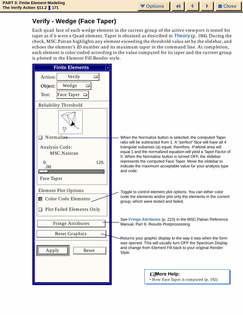
CloseOptionsPART 3: Finite Element ModelingThe Verify Action §11.2 171 Options
Verify - Wedge (Face Taper)Each quad face of each wedge element in the current group of the active viewport is tested for taper as if it were a Quad element. Taper is obtained as described in Theory (p. 184). During the check, MSC.Patran highlights any element exceeding the threshold value set by the slidebar, and echoes the element’s ID number and its maximum taper in the command line. At completion, each element is color-coded according to the value computed for its taper and the current group is plotted in the Element Fill Render style.
When the Normalize button is selected, the computed Taper ratio will be subtracted from 1. A “perfect” face will have all 4 triangular subareas (a) equal, therefore, 4*a⁄total area will equal 1 and the normalized equation will yield a Taper Factor of 0. When the Normalize button is turned OFF, the slidebar represents the computed Face Taper. Move the slidebar to indicate the maximum acceptable value for your analysis type and code.
• How Face Taper is computed (p. 192) ☞ More Help:
Returns your graphic display to the way it was when the form was opened. This will usually turn OFF the Spectrum Display and change from Element Fill back to your original Render Style.
Finite Elements
Action: Verify
Object: Object: Wedge
Test: Face Taper
Reliability Threshold
Normalize
Analysis Code: MSC.Nastran
120. 0.
Element Plot Options
Color Code Elements
Plot Failed Elements Only
.00
Face Taper
a4 aA
Toggle to control element plot options. You can either color code the elements and/or plot only the elements in the current group, which were tested and failed.
Reset Graphics
Apply Reset
Fringe AttributesSee Fringe Attributes (p. 223) in the MSC.Patran Reference Manual, Part 6: Results Postprocessing.

CloseOptionsPART 3: Finite Element ModelingThe Verify Action §11.2 172 Options
Verify - Hex (All)Each hex element in the current group of the active viewport is tested for each of the hex verification tests.
Finite Elements
Verify Action:
Hex Object:
All Test:
Normalize
Analysis Code: MSC.Nastran
Aspect Ratio :5.0
Edge Angle: 30.
Face Skew: 30.
Face Warp: 7.
Twist: 45.
Face Taper: 0.8
Normal Offset: 0.15
Tangent Offset 0.15
Reliability Threshold
Apply
When the Apply button is selected, a spreadsheet will be displayed showing the worst case value for each test and the element at which it occurs.
☞ More Help: • Spreadsheet Information (p. 173) • Test Definitions (p. 184)

CloseOptionsPART 3: Finite Element ModelingThe Verify Action §11.2 173 Options
Verify - Hex (All) Spreadsheet
Hex Verification Summary
Test Number Failed Worst Case At Element
Aspect
Edge Angle
Face Skew 1
40
4 Max=1.9266015
Max=32.110462
Max=29.615601 154
186
203
This column lists the Verification test. All tests listed on the application form will be performed. Use the scroll bar to view additional tests.
The last two columns list the maximum (or minimum, if applicable) value of the test and the element at which this worst case occurs.
This column lists the number of elements in the current group that exceeded the reliability threshold shown on the application form.
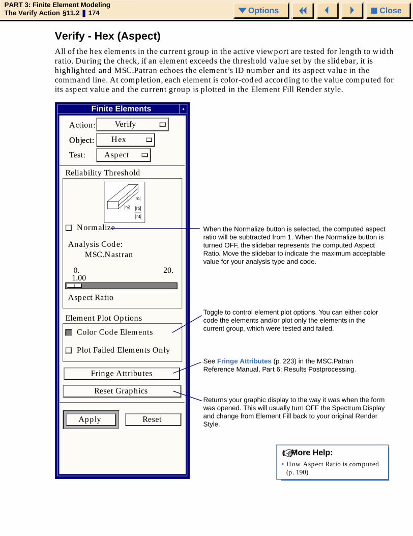
CloseOptionsPART 3: Finite Element ModelingThe Verify Action §11.2 174 Options
Verify - Hex (Aspect)All of the hex elements in the current group in the active viewport are tested for length to width ratio. During the check, if an element exceeds the threshold value set by the slidebar, it is highlighted and MSC.Patran echoes the element’s ID number and its aspect value in the command line. At completion, each element is color-coded according to the value computed for its aspect value and the current group is plotted in the Element Fill Render style.
When the Normalize button is selected, the computed aspect ratio will be subtracted from 1. When the Normalize button is turned OFF, the slidebar represents the computed Aspect Ratio. Move the slidebar to indicate the maximum acceptable value for your analysis type and code.
• How Aspect Ratio is computed (p. 190)
☞ More Help:
Returns your graphic display to the way it was when the form was opened. This will usually turn OFF the Spectrum Display and change from Element Fill back to your original Render Style.
Finite Elements
Action: Verify
Object: Object: Hex
Test: Aspect
Reliability Threshold
Normalize
Analysis Code: MSC.Nastran
20. 0.
Element Plot Options
Color Code Elements
Plot Failed Elements Only
1.00
Aspect Ratio
h2
h1
h2
h1
Toggle to control element plot options. You can either color code the elements and/or plot only the elements in the current group, which were tested and failed.
Reset Graphics
Apply Reset
Fringe Attributes
See Fringe Attributes (p. 223) in the MSC.Patran Reference Manual, Part 6: Results Postprocessing.

CloseOptionsPART 3: Finite Element ModelingThe Verify Action §11.2 175 Options
Verify - Hex (Edge Angle)The maximum edge angle is calculated for each hex element in the current group. Edge angle is obtained as described in Theory (p. 184). During the check, MSC.Patran highlights any element exceeding the threshold value set by the slidebar, and echoes the element’s ID number and its maximum edge angle in the command line. At completion, each element is color-coded according to the value computed for its edge angle and the current group is plotted in the Element Fill Render style.
When the Normalize button is selected, the computed taper ratio will be divided by 90°. When the Normalize button is turned OFF, the slidebar represents the computed Edge Angle. Move the slidebar to indicate the maximum acceptable value for your analysis type and code.
Returns your graphic display to the way it was when the form was opened. This will usually turn OFF the Spectrum Display and change from Element Fill back to your original Render Style.
Finite Elements
Action: Verify
Object: Object: Hex
Test: Edge Angle
Reliability Threshold
Normalize
Analysis Code: MSC.Nastran
90. 0.
Element Plot Options
Color Code Elements
Plot Failed Elements Only
.00
Edge Angle
α
Max (90× α )°-
Toggle to control element plot options. You can either color code the elements and/or plot only the elements in the current group, which were tested and failed.
Reset Graphics
Apply Reset
Fringe AttributesSee Fringe Attributes (p. 223) in the MSC.Patran Reference Manual, Part 6: Results Postprocessing.
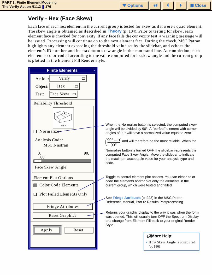
CloseOptionsPART 3: Finite Element ModelingThe Verify Action §11.2 176 Options
Verify - Hex (Face Skew)Each face of each hex element in the current group is tested for skew as if it were a quad element. The skew angle is obtained as described in Theory (p. 184). Prior to testing for skew, each element face is checked for convexity. If any face fails the convexity test, a warning message will be issued. Processing will continue on to the next element face. During the check, MSC.Patran highlights any element exceeding the threshold value set by the slidebar, and echoes the element’s ID number and its maximum skew angle in the command line. At completion, each element is color-coded according to the value computed for its skew angle and the current group is plotted in the Element Fill Render style.
When the Normalize button is selected, the computed skew angle will be divided by 90°. A “perfect” element with corner angles of 90° will have a normalized value equal to zero
and will therefore be the most reliable. When the
Normalize button is turned OFF, the slidebar represents the computed Face Skew Angle. Move the slidebar to indicate the maximum acceptable value for your analysis type and code.
90° α–90°------------------
• How Skew Angle is computed (p. 186)
☞ More Help:
Returns your graphic display to the way it was when the form was opened. This will usually turn OFF the Spectrum Display and change from Element Fill back to your original Render Style.
Finite Elements
Action: Verify
Object: Object: Hex
Test: Face Skew
Reliability Threshold
Normalize
Analysis Code: MSC.Nastran
90. 0.
Element Plot Options
Color Code Elements
Plot Failed Elements Only
.00
Face Skew Angle
(90× α )°-
α
Toggle to control element plot options. You can either color code the elements and/or plot only the elements in the current group, which were tested and failed.
Reset Graphics
Apply Reset
Fringe Attributes
See Fringe Attributes (p. 223) in the MSC.Patran Reference Manual, Part 6: Results Postprocessing.
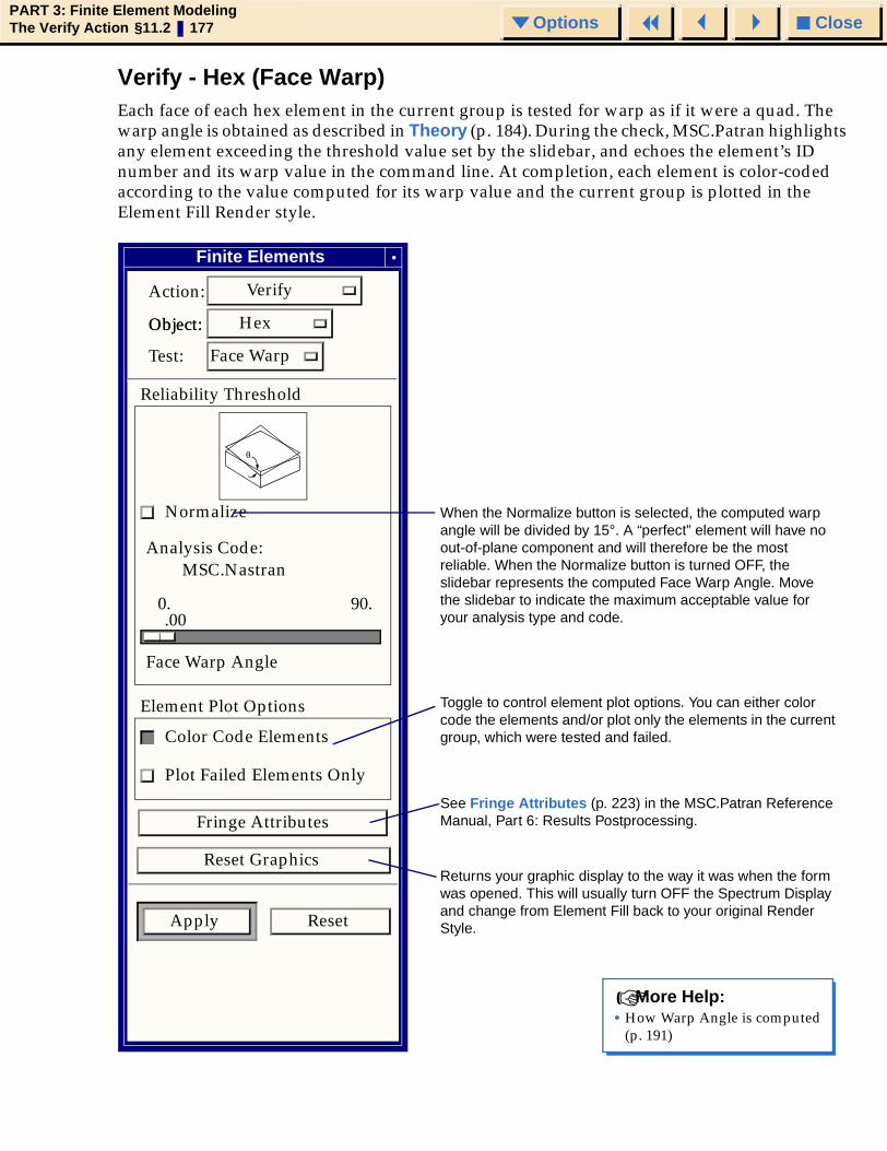
CloseOptionsPART 3: Finite Element ModelingThe Verify Action §11.2 177 Options
Verify - Hex (Face Warp)Each face of each hex element in the current group is tested for warp as if it were a quad. The warp angle is obtained as described in Theory (p. 184). During the check, MSC.Patran highlights any element exceeding the threshold value set by the slidebar, and echoes the element’s ID number and its warp value in the command line. At completion, each element is color-coded according to the value computed for its warp value and the current group is plotted in the Element Fill Render style.
When the Normalize button is selected, the computed warp angle will be divided by 15°. A “perfect” element will have no out-of-plane component and will therefore be the most reliable. When the Normalize button is turned OFF, the slidebar represents the computed Face Warp Angle. Move the slidebar to indicate the maximum acceptable value for your analysis type and code.
• How Warp Angle is computed (p. 191)
☞ More Help:
Returns your graphic display to the way it was when the form was opened. This will usually turn OFF the Spectrum Display and change from Element Fill back to your original Render Style.
Finite Elements
Action: Verify
Object: Object: Hex
Test: Face Warp
Reliability Threshold
Normalize
Analysis Code:MSC.Nastran
90. 0.
Element Plot Options
Color Code Elements
Plot Failed Elements Only
.00
Face Warp Angle
θ
Toggle to control element plot options. You can either color code the elements and/or plot only the elements in the current group, which were tested and failed.
Reset Graphics
Apply Reset
Fringe AttributesSee Fringe Attributes (p. 223) in the MSC.Patran Reference Manual, Part 6: Results Postprocessing.

CloseOptionsPART 3: Finite Element ModelingThe Verify Action §11.2 178 Options
Verify - Hex (Twist)Each hex element in the current group is tested for maximum twist angle. Twist is obtained as described in Theory (p. 184). During the check, MSC.Patran highlights any element exceeding the threshold value set by the slidebar, and echoes the element’s ID number and its maximum twist in the command line. At completion, each element is color-coded according to the value computed for its twist and the current group is plotted in the Element Fill Render style.
When the Normalize button is selected, the computed twist angle will be divided by 90°. When the Normalize button is turned OFF, the slidebar represents the computed Twist Angle. Move the slidebar to indicate the maximum acceptable value for your analysis type and code.
• How Twist is computed (p. 196)☞ More Help:
Returns your graphic display to the way it was when the form was opened. This will usually turn OFF the Spectrum Display and change from Element Fill back to your original Render Style.
Finite Elements
Action: Verify
Object: Object: Hex
Test: Twist
Reliability Threshold
Normalize
Analysis Code: MSC.Nastran
90. 0.
Element Plot Options
Color Code Elements
Plot Failed Elements Only
.00
Twist Angle
θ
Toggle to control element plot options. You can either color code the elements and/or plot only the elements in the current group, which were tested and failed.
Reset Graphics
Apply Reset
Fringe Attributes
See Fringe Attributes (p. 223) in the MSC.Patran Reference Manual, Part 6: Results Postprocessing.

CloseOptionsPART 3: Finite Element ModelingThe Verify Action §11.2 179 Options
Verify - Hex (Face Taper)Each face of each hex element in the current group is tested for taper as if it were a quad element. Taper is obtained as described in Theory (p. 184). During the check, MSC.Patran highlights any element exceeding the threshold value set by the slidebar, and echoes the element’s ID number and its maximum taper in the command line. At completion, each element is color-coded according to the value computed for its taper and the current group is plotted in the Element Fill Render style.
When the Normalize button is selected, the computed taper ratio will be subtracted from 1. A “perfect” element face will have all 4 triangular subareas (a) equal, therefore 4*a⁄total area will equal 1 and the normalized equation will yield a Taper Factor of 0.
When the Normalize button is turned OFF, the slidebar represents the computed Taper Ratio. Move the slidebar to indicate the maximum acceptable value for your analysis type and code.
Returns your graphic display to the way it was when the form was opened. This will usually turn OFF the Spectrum Display and change from Element Fill back to your original Render Style.
Finite Elements
Action: Verify
Object: Object: Hex
Test: Face Taper
Reliability Threshold
Normalize
Analysis Code: MSC.Nastran
1. 0.
Element Plot Options
Color Code Elements
Plot Failed Elements Only
.00
Face Taper
a4 aA
Toggle to control element plot options. You can either color code the elements and/or plot only the elements in the current group, which were tested and failed.
Reset Graphics
Apply Reset
Fringe AttributesSee Fringe Attributes (p. 223) in the MSC.Patran Reference Manual, Part 6: Results Postprocessing.
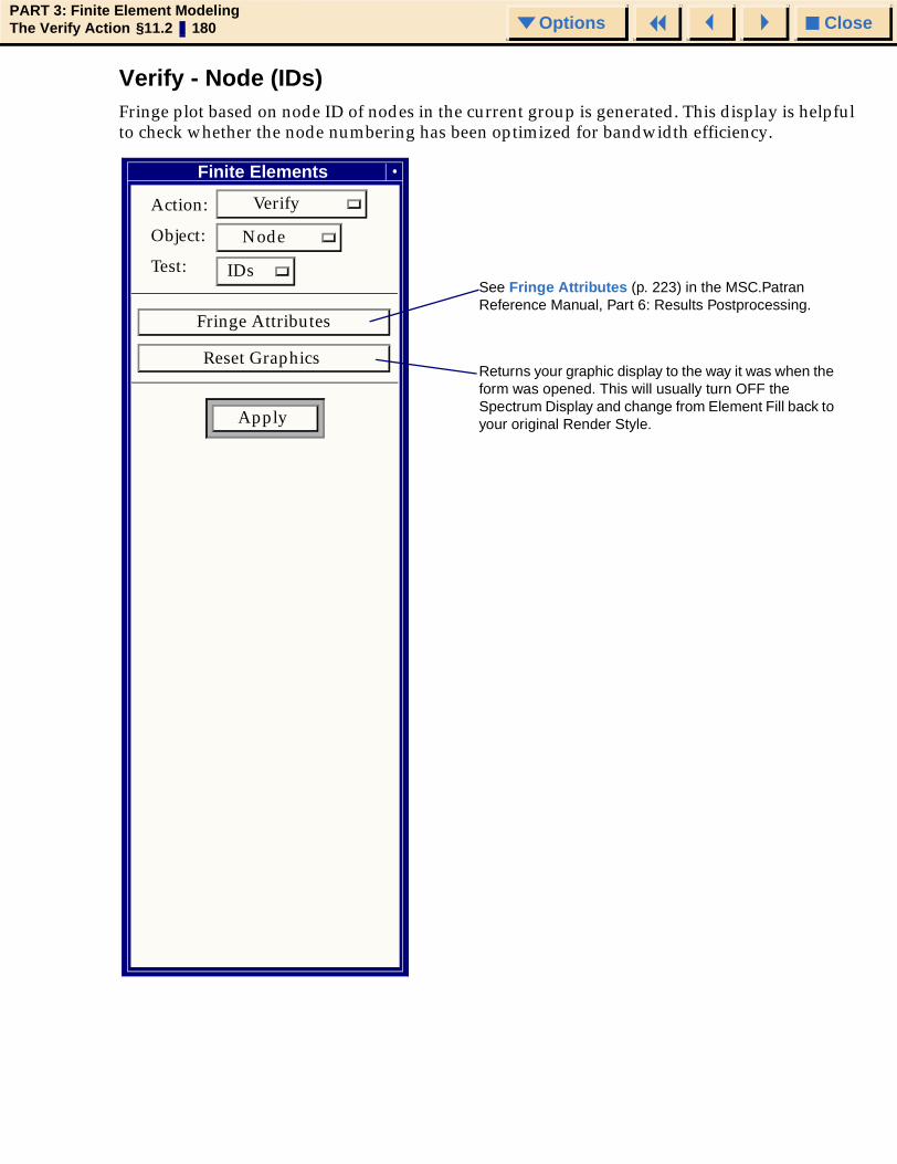
CloseOptionsPART 3: Finite Element ModelingThe Verify Action §11.2 180 Options
Verify - Node (IDs)Fringe plot based on node ID of nodes in the current group is generated. This display is helpful to check whether the node numbering has been optimized for bandwidth efficiency.
Finite Elements
Verify Action:
Node Object:
IDs Test:
Apply
Returns your graphic display to the way it was when the form was opened. This will usually turn OFF the Spectrum Display and change from Element Fill back to your original Render Style.
Reset Graphics
Fringe Attributes
See Fringe Attributes (p. 223) in the MSC.Patran Reference Manual, Part 6: Results Postprocessing.

CloseOptionsPART 3: Finite Element ModelingThe Verify Action §11.2 181 Options
Verify - Midnode (Normal Offset)All quadratic order elements (those with mid-side nodes) in the current group are tested for deviation of the mid-side node from the mid-node position for an element with no curvature. The offset distance is measured perpendicular to a line that is the shortest distance between the corner nodes of that edge.
Finite Elements
Verify Action:
Midnode Object:
Normal Offset Test:
Analysis Code:MSC.Nastran
Normal Offset
Most Least
Reliability Threshold
During the check, MSC.Patran highlights any element exceeding the threshold value set by the slidebar, and echoes the element’s ID number and its Normal Offset value in the command line. At completion, each element is color-coded according its Normal Offset value. All elements exceeding the threshold value will be colored red. The current group is plotted in the Element Fill Render style.
Set the slidebar to an acceptable offset value for your analysis code. A “perfect” element will have the mid-side node directly at the mid-edge position, therefore, the offset d=0. The equation will yield a value of zero and indicates the most reliable element for analysis.
2dL------.00
d
L2dL
Returns your graphic display to the way it was when the form was opened. This will usually turn OFF the Spectrum Display and change from Element Fill back to your original Render Style, and removing the vendor display from the viewport.
Element Plot Options
Color Code Elements
Plot Failed Elements Only
Toggle to control element plot options. You can either color code the elements and/or plot only the elements in the current group, which were tested and failed.
Reset Graphics
Apply Reset
Fringe AttributesSee Fringe Attributes (p. 223) in the MSC.Patran Reference Manual, Part 6: Results Postprocessing.

CloseOptionsPART 3: Finite Element ModelingThe Verify Action §11.2 182 Options
Verify - Midnode (Tangent Offset)All quadratic order elements (those with mid-side nodes) in the current group in the active viewport are tested for deviation of the mid-side node from the mid-edge position of the element. The offset distance is measured along a line that is the shortest distance between the corner nodes of that edge.
Finite Elements
Verify Action:
Midnode Object:
Tangent Offset Test:
Analysis Code: MSC.Nastran
Tangent Offset
Most Least
Reliability Threshold
Returns your graphic display to the way it was when you entered the form. This will usually entail changing from Element Fill back to your original Render Style and removing the spectrum display from your viewport.
During the check, MSC.Patran highlights any element exceeding the threshold value set by the slidebar, and echoes the element’s ID number and its Tangent Offset value in the Command Line. At completion, each element is color-coded according its Tangent Offset value. All elements exceeding the threshold value will be colored red. The current group is plotted in the Element Fill Render style.
Set the slidebar to an acceptable offset value for your analysis code. A “perfect” element will have the mid-side node directly at the mid-edge position; therefore, the offset d=0. The equation will yield a value of zero and indicates the most reliable element for analysis.
2dL------
.00
d
L2dL
Element Plot Options
Color Code Elements
Plot Failed Elements Only
Toggle to control element plot options. You can either color code the elements and/or plot only the elements in the current group, which were tested and failed.
Reset Graphics
Apply Reset
Fringe Attributes See Fringe Attributes (p. 223) in the MSC.Patran Reference Manual, Part 6: Results Postprocessing.
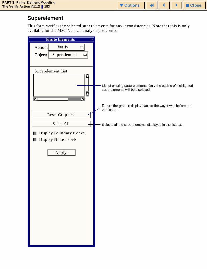
CloseOptionsPART 3: Finite Element ModelingThe Verify Action §11.2 183 Options
SuperelementThis form verifies the selected superelements for any inconsistencies. Note that this is only available for the MSC.Nastran analysis preference.
Action: Verify
Object: Object: Object: Superelement Object: Object: Object: Object: Object: Object:
Superelement List
Reset Graphics
Display Boundary Nodes
-Apply-
Finite Elements
List of existing superelements. Only the outline of highlighted superelements will be displayed.
Return the graphic display back to the way it was before the verification.
Select All
Display Node Labels
Selects all the superelements displayed in the listbox.

CloseOptionsPART 3: Finite Element ModelingThe Verify Action §11.3 184 Options
11.3 Theory
Skew
Tria. Three potential skew angles are computed for each tria element. To calculate each skew angle, two vectors are constructed: one from a vertex to the mid-point of the opposite edge, and the other between the mid-points of the adjacent edges. The difference is taken of the angle between these two vectors and 90°. This procedure is repeated for the other two vertices. The largest of the three computed angles is reported as the skew angle for that element.
If Normalize is selected on the verification form, the skew angle is divided by 90° to yield the skew factor. An equilateral triangle will have a skew factor of 0.
Figure 11-2 Tria Skew Angle
Quad. Prior to testing for skew, each element is first checked for convexity. Elements which fail the convexity check “double back” on themselves causing their element stiffness terms to have either a zero or negative value.
Figure 11-3 Convexity Check
α
Skew Angle = 90° - α
Skew Factor = (90° - α)/90°
21
3 4
Single Re-entrant AngleIncorrect nodal sequencing
Double Re-entrant angle

CloseOptionsPART 3: Finite Element ModelingThe Verify Action §11.3 185 Options
This skew test is based on a reference frame created by first bisecting the four element edges, creating an origin at the vector average of the corners, where the x-axis extends from the origin to the bisector on edge 2. The z-axis is in the direction of the cross product of the x-axis and the vector from the origin to the bisector of edge 3. The y-axis is in the direction of the cross product of the x and z axis as shown in Figure 11-4.
Figure 11-4 The Element Test Coordinate System
The Robinson and Haggenmacher1 skew test uses the angle alpha between the edge 2 and 4 bisector and the test y-axis. The resulting angle is subtracted from 90° to yield the skew angle.
If Normalize is selected on the verification form, the skew angle is divided by 90° to yield the skew factor. A square element will have a skew factor of 0.
Figure 11-5 Quad Skew Angle
Tet. Each face of the tet element is tested for skew as if it were a tria element. See explanation for computation of skew angle - Tria (p. 184). The highest resulting angle for each element is retained as the skew angle.
1J. Robinson and G. W. Haggenmacher, “Element Warning Diagnostics,” Finite Element News, June and August, 1982.
Node 4
Edge 3
Node 3
Edge 2
Node 2
Edge 1
Node 1
Edge 4 z
y
x
α
90 α°-

CloseOptionsPART 3: Finite Element ModelingThe Verify Action §11.3 186 Options
Wedge. Each face of the wedge element is tested for skew as if it were either a quad or tria element. See explanation for computation of skew angle - Tria (p. 184) or Quad (p. 184). The highest resulting angle for each element is retained as the skew angle.
Hex. Each face of the hex element is tested for skew as if it were a quad element. See explanation for computation of skew angle - Quad (p. 184). The highest resulting angle for each element is retained as the skew angle.

CloseOptionsPART 3: Finite Element ModelingThe Verify Action §11.3 187 Options
Aspect Ratio
Tria. The aspect ratio for a triangle is calculated as the ratio of the length, h2, of the edge of a triangle, to the height, h1. The ratio of h2 to h1 is then multiplied by such that a “perfect” element in the shape of an equilateral triangle will equal one. This procedure is repeated for the remaining two edges of the triangle, and the largest value is retained as the aspect ratio for the element.
If Normalize is selected on the verification form, then the aspect ratio is inverted such that it becomes less than or equal to one. This inverted aspect ratio is subtracted from one to yield the aspect factor. An equilateral triangle will have an aspect factor of 0.
Figure 11-6 Tria Aspect Ratio
Quad. The aspect ratio for a quad is derived from one test proposed by Robinson and Haggenmacher1. This test is based on projection plane created by first bisecting the four element edges, creating a point on the plane at the vector average of the corners. The x-axis extends from the point to the bisector on edge 2. The ratio is determined as the ratio of the length from the origin to the bisector of edge 2 and the length from the origin to the bisector of edge 3. If the ratio is less than 1.0, it is inverted.
1J. Robinson and G. W. Haggenmacher, “Element Warning Diagnostics,” Finite Element News, June and August, 1982.
3 2⁄
h1
h2
Aspect Ratio = 3h2
2h1------------- Aspect Factor =
2h1
3h2
-------------–

CloseOptionsPART 3: Finite Element ModelingThe Verify Action §11.3 188 Options
If Normalize is selected on the verification form, then the aspect ratio is inverted such that it becomes less than or equal to one. This inverted aspect ratio is subtracted from one to yield the normalized aspect ratio. A square element will have a normalized aspect ratio of 0.
Figure 11-7 Quad Aspect Ratio
Tet. The aspect ratio for a tet element is computed by taking the ratio of the height of a vertex to the square root of the area of the opposing face. This value is then manipulated in one of two ways, depending on whether the Normalize parameter is selected on the verification form.
If Normalize is NOT selected, the maximum height to area value is multiplied by a factor , which is the ratio of height to edge length for an equilateral tetrahedron. This
result is reported as the Aspect Ratio. An equilateral tet will report a value of 1. Aspect Ratio = .
If Normalize IS selected, the maximum height to area value is inverted and subtracted from 1. Aspect Factor = .
Figure 11-8 Tet Aspect Ratio
Node 4
Edge 3
Node 3
Edge 2
Node 2
Edge 1
Node 1
Edge 4
h1
h2
h1
h2, h1 > h2
h2
h1, h2 > h1
Aspect Ratio =
C 0.805927=
Max Cf hi⋅ Ai⁄( ), i = 1, 2, 3, 4
1 1– MaxCf hi⋅ Ai⁄( )⁄( ), i = 1, 2, 3, 4
Max (cƒ. h i ⁄√Ai)cƒ = .805927
hi
Ai

CloseOptionsPART 3: Finite Element ModelingThe Verify Action §11.3 189 Options
Wedge. MSC.Patran averages the two triangular faces of the wedge element to obtain a mid-
surface. The aspect ratio of this triangular mid-surface is computed . Next the height
(h1) of the wedge is compared to the maximum edge length of the mid-surface (h4).
If the height of the wedge is greater than the maximum edge length then the aspect ratio for the wedge element equals the mid-surface aspect ratio multiplied by the maximum edge length divided by the distance between the triangular faces (h3).
If the height of the wedge is less than the maximum edge length then the aspect ratio for the wedge element equals either the mid-surface aspect ratio or the maximum edge length divided by the distance between the triangular faces, whichever is greater.
If Normalize is selected on the verification form, then the aspect ratio is inverted such that it becomes less than or equal to one. This inverted aspect ratio is subtracted from one to yield the aspect factor. An equilateral wedge element will have an aspect factor of 0.
Figure 11-9 Wedge Aspect Ratio
3h2 2h1⁄( )
h4
h3
h2
h1
Aspect Ratio = h4 √3h2
h3 2h1
Aspect Fact or= 1 -h3
√3h2h4
2h1

CloseOptionsPART 3: Finite Element ModelingThe Verify Action §11.3 190 Options
Hex. The aspect ratio is calculated as the ratio of the distance between opposing faces. This distance is determined by treating each HEX face as if it were a warped quadrilateral. Each face is processed to produce a projected plane. The distances between the centerpoints of all three pairs of opposing faces are compared.The aspect ratio is determined by taking the maximum distance between any two faces and dividing it by the minimum distance between any two faces.
If Normalize is selected on the verification form, then the aspect ratio is inverted such that it becomes less than or equal to one. This inverted aspect ratio is subtracted from one to yield the aspect factor. A cubic element will have an aspect factor of 0.
Figure 11-10 Hex Aspect Ratio
h1h2 h3
AspectFactor 1min h1 h2 h3, ,( )max h1 h2 h3, ,( )-------------------------------------------–=AspectRatio
max h1 h2 h3, ,( )min h1 h2 h3, ,( )-------------------------------------------=

CloseOptionsPART 3: Finite Element ModelingThe Verify Action §11.3 191 Options
Warp
Quad. The warp test is a test proposed by Robinson and Haggenmacher1 which uses the following method of calculating the Quad element Warp. This test is based on a projection plane created by first bisecting the four element edges, creating a point on the plane at the vector average of the corners, where the x-axis extends from the point to the bisector on edge 2. The plane normal is in the direction of the cross product of the x-axis and the vector from the origin to the bisector of edge 3. Every corner of the quad will then be a distance “h” from the plane. The length of each half edge is measured and the shortest length is assigned “l.” The warp angle is the arcsine of the ratio of the projection height “h” to the half edge length “l.”
If Normalize is selected on the verification form, the warp angle is divided by 15° to yield the warp factor. A planar element has a warp factor of 0.
Figure 11-11 Quad Warp Angle
Wedge. Each quad face of the wedge element is tested for warp as if it were a quad element. See explanation for computation of warp angle - Quad (p. 191). The highest resulting angle for each element is retained as the warp angle.
Hex. Each face of the hex element is tested for warp as if it were a quad element. See explanation for computation of warp angle - Quad (p. 191). The highest resulting angle for each element is retained as the warp angle.
1J. Robinson and G. W. Haggenmacher, “Element Warning Diagnostics,” Finite Element News, June and August, 1982.
Node 4
Edge 3
Node 3
Edge 2
Node 2
Edge 1
Node 1
Edge 4 z
y
x
h
l
= sin-1
lhθ
θ

CloseOptionsPART 3: Finite Element ModelingThe Verify Action §11.3 192 Options
Taper
Quad. The taper test is a test proposed by Robinson and Haggenmacher1 which uses the following method of calculating the Quad element. Taper four triangles are created bounded by the element edge and the edges created by connecting the element verification reference frame origin with the two nodes at the element edge. The resulting four triangular areas are calculated and then summed. The ratio of the area with the smallest triangle and the total area of the element is taken as the taper ratio.
If Normalize is selected on the verification form, the taper ratio is subtracted from one to yield the taper factor. A square element has a taper factor of 0.
Figure 11-12 Quad Taper
Wedge. Each quad face of the wedge element is tested for taper as if it were a quad element. See explanation for computation of taper - Quad (p. 192). The lowest resulting value for each element is retained as the value of face taper.
Hex. Each face of the hex element is tested for taper as if it were a quad element. See explanation for computation of taper - Quad (p. 192). The lowest resulting value for each element is retained as the value of face taper.
a1a2
a4
a3
Taper Ratio = 4asmallest
1 a2 a3 a4+ + +----------------------------------------------

CloseOptionsPART 3: Finite Element ModelingThe Verify Action §11.3 193 Options
Edge Angle
Tet. Edge angle measures the angle between adjacent faces of the tetrahedral element. In an equilateral tetrahedral element, this angle will equal 70.259°. The largest angle found in the element is retained. MSC.Patran then computes the absolute value of the difference between the measured angle and 70.259°. This is the value reported as the Edge Angle.
If Normalize is selected on the verification form, the edge angle is divided by 110° to yield the edge angle factor. An equilateral tet will have an edge angle factor of 0.
Figure 11-13 Tet Edge Angle
Edge Angle = 70.529° - α
Edge Angle Factor = (70.529° - α) / 110°
- 70.53
α
α °

CloseOptionsPART 3: Finite Element ModelingThe Verify Action §11.3 194 Options
Wedge. An edge angle is the absolute value of the angle between the two faces meeting at an edge subtracted from the ideal angle for that edge. The ideal angle between two quad faces is 60 degrees, and the ideal angle between a quad face and a tria face is 90 degrees. For warped quad faces, the projected plane of the face is used to compute the face normal used in the angle calculation. The maximum edge angle is calculated for each wedge element.
If Normalize is selected on the verification form, the edge angle is divided by 60° to yield the edge angle factor.
Figure 11-14 Wedge Edge Angle
Hex. An edge angle is the absolute value of the angle between the two faces meeting at an edge subtracted from the ideal angle for that edge. The ideal angle between faces of a hex element is 90 °. For warped faces, the projected planes for each face is used to compute the face normals used in the angle calculation. The maximum edge angle is calculated for each hex element.
If Normalize is selected on the verification form, the edge angle is divided by 90° to yield the edge angle factor.
Figure 11-15 Hex Edge Angle
Edge Angle = Max (600 - θ, 900 - α)
Edge Angle Factor = [Max (600 - θ, 900 - α)] / 600
α
θ
Max (60° − θ, 90° - α)
Edge Angle = Max (90° - α)
Edge Angle Factor = [Max (90° - α)] / 90°
α
×Max (90° - α)

CloseOptionsPART 3: Finite Element ModelingThe Verify Action §11.3 195 Options
Collapse
Tet. Collapse is an indicator of near zero volume tetrahedral elements. The test takes the ratio of the height of a vertex to the square root of the area of the opposing face. This value approaches zero as the volume of the element approaches zero.
If Normalize is NOT selected on the verification form, the minimum height to area value is multiplied by a factor Cf = 0.805927, which is the ratio of height to edge length for an equilateral
tetrahedron. An equilateral tet will report a value of 1. Collapse = .
If Normalize IS selected, the minimum height to area value is subtracted from 1. An equilateral
tet will report a value of 0. Collapse Factor = , i = 1,2,3,4.
Figure 11-16 Tet Collapse
MinCf hi×
Ai
------------------
, i 1 2 3 4, , ,=
MinCf hi×
Ai
------------------
–
hi
Ai
Min (h i ⁄ √ A i )

CloseOptionsPART 3: Finite Element ModelingThe Verify Action §11.3 196 Options
Twist
Wedge. Twist is the rotation of one face of a solid with respect to its opposite face. To compute twist angle, normals are drawn from the center of each tria surface. These vectors are projected onto a plane. The angular difference between the two vectors is the twist angle.
If Normalize is selected on the verification form, the twist angle is divided by 60° to yield the twist factor.
Figure 11-17 Wedge Twist Angle
Hex. Twist is the rotation of one face of a solid with respect to its opposite face. A twist angle is computed about all three principal axes of hex elements. To compute the twist angle, each face is treated as if it were a warped quad. Vectors from the center of the projected plane to the middle of two adjacent edges are constructed. The vectors are summed to compute a reference vector. The same steps are performed for the opposite face. A line through the center of each projected face and the plane normal to this line is determined. The two reference vectors are projected onto this plane and the angular difference between them is measured. The highest angle found is retained as the twist angle.
θ
•
•• •
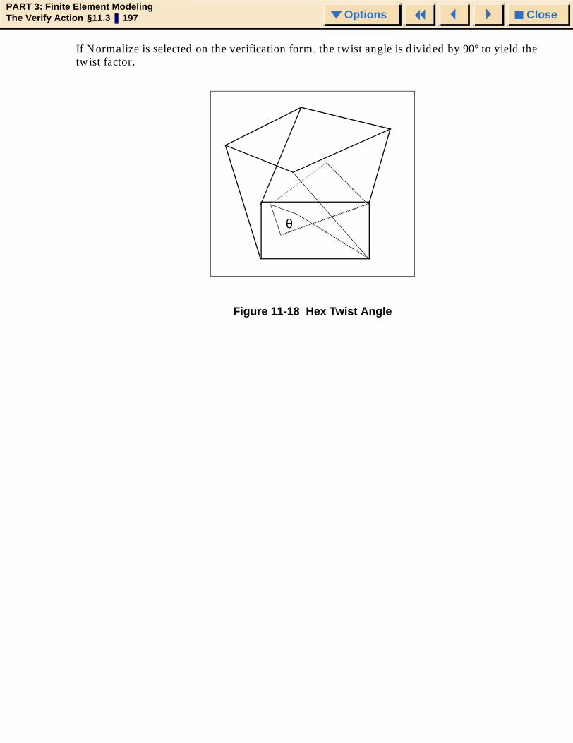
CloseOptionsPART 3: Finite Element ModelingThe Verify Action §11.3 197 Options
If Normalize is selected on the verification form, the twist angle is divided by 90° to yield the twist factor.
Figure 11-18 Hex Twist Angle
θ

CloseOptionsPART 3: Finite Element ModelingThe Verify Action §11.3 198 Options

CloseOptionsPART 3: Finite Element ModelingThe Show Action... § 199 Options
MSC.Patran Reference Manual, Part 3: Finite Element Modeling
CHAPTER
12 The Show Action
■ Show Forms
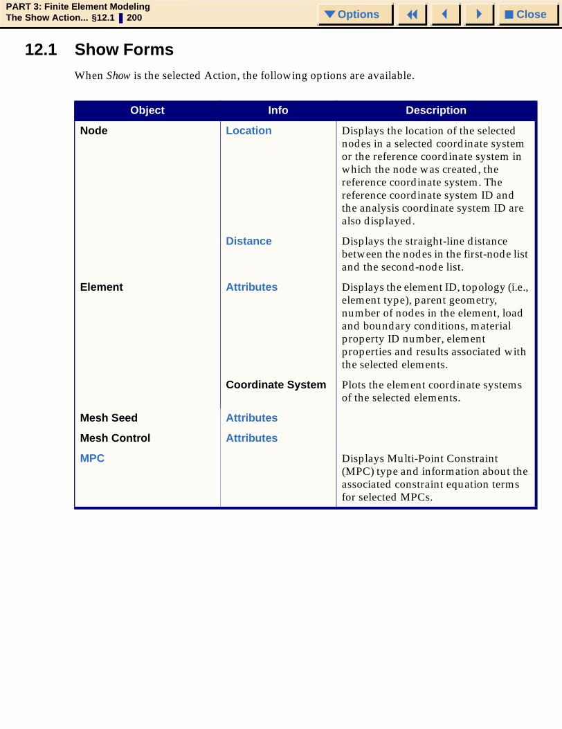
CloseOptionsPART 3: Finite Element ModelingThe Show Action... §12.1 200 Options
12.1 Show FormsWhen Show is the selected Action, the following options are available.
Object Info Description
Node Location Displays the location of the selected nodes in a selected coordinate system or the reference coordinate system in which the node was created, the reference coordinate system. The reference coordinate system ID and the analysis coordinate system ID are also displayed.
Distance Displays the straight-line distance between the nodes in the first-node list and the second-node list.
Element Attributes Displays the element ID, topology (i.e., element type), parent geometry, number of nodes in the element, load and boundary conditions, material property ID number, element properties and results associated with the selected elements.
Coordinate System Plots the element coordinate systems of the selected elements.
Mesh Seed Attributes
Mesh Control Attributes
MPC Displays Multi-Point Constraint (MPC) type and information about the associated constraint equation terms for selected MPCs.

CloseOptionsPART 3: Finite Element ModelingThe Show Action... §12.1 201 Options
Show - Node LocationWhen Show is the selected Action and Node is the selected Object, the Show Node menu is displayed. This is used to view either the location of or distance between selected nodes.
The Node Summary table lists information about the existing nodes in the current database, including the highest node ID currently used, the total number of nodes in the model, the number of unreferenced nodes, and the total number of nodes in the current group.
The Node List textbox is where the list of nodes to be shown is specified. Nodes can be specified by selecting this box and then selecting the nodes with the cursor, or by typing in “node n” where n is the number of the desired node.
Finite Elements The Show Node Location menu displays the location of the selected nodes in the reference coordinate system, giving the reference coordinate system ID, and the analysis coordinate system ID.
More detailed information than what is provided in the resulting information table can be obtained by selecting the individual cells of the The Show Action Information Form (p. 569) in the MSC.Patran Reference Manual, Part 2: Geometry Modeling. This additional information is then displayed in the textbox directly below the table.
Used to input the coordinate frame in which the coordinate values of the selected nodes are to be shown. Coordinate frames can be specified by selecting this box and then cursor selecting, or by typing “Coord n” where n is the ID of the desired coordinate frame. If no coordinate frame is specified, the nodes will be shown in the coordinate frame in which they were created.
See Write to Report (p. 204)
Action: Show
Object:
Info:
Node
Location
Node Summary
Last ID: 0
Total in Model: 0
Total Unreferenced: 0
Total in 'default_group’:0
Write to Report
Coordinate Frame
Auto Execute
Node List
Apply

CloseOptionsPART 3: Finite Element ModelingThe Show Action... §12.1 202 Options
Show - Node DistanceWhen Show is the selected Action and Node is the selected Object, the Show Node menu is displayed. This is used to view either the location of or distance between selected nodes.
The Node Summary table lists information about the existing nodes in the current database, including the highest node ID currently used, the total number of nodes in the model, the number of unreferenced nodes and the total number of nodes in the current group.
The First Node List textbox is used to input the list of nodes where the distance measurement starts. Nodes can be specified by selecting this box and then selecting the nodes with the cursor, or by typing in “node n” where n is the number of the desired node.
The Show Node Distance menu displays the straight-line distance between the nodes in the first-node list and the second-node list.
More detailed information than what is provided in the resulting information table can be obtained by selecting the individual cells of the The Show Action Information Form (p. 569) in the MSC.Patran Reference Manual, Part 2: Geometry Modeling. This additional information is then displayed in the textbox directly below the table.
The Second Node List textbox is used to input the list of nodes where the distance measurement ends. If the lists do not contain the same number of points, the last point of the shorter list will be repeated until the longer list is exhausted.
See Write to Report (p. 204).
Finite Elements Action: Show
Object:
Info:
Node
Distance
Node Summary
Last ID: 0
Total in Model: 0
Total Unreferenced: 0
Total in 'default_group' : 0
Auto Execute
First Node List
Second Node List
Apply
Write to Report

CloseOptionsPART 3: Finite Element ModelingThe Show Action... §12.1 203 Options
Show - Element AttributesWhen Show is the selected Action, Element is the selected Object and Attributes is the selected Info, the Show Element Attributes menu is displayed. This is used to display the element attributes of selected elements.
Finite Elements
Action: Show
Object: Element
Info: Attributes
Element SummaryLast ID:
0Total in Model:
0Total in 'default_group' :
0
Write to Report
Auto Execute
Apply
Element List
The Element Summary table lists information about the existing elements in the current database including the highest ID number currently used, the total number of elements in the model, and the total number of elements in the current group.
The Element List textbox is where the list of elements to be shown is specified. Elements can be specified by using the mouse button on this box, and then selecting the elements with the cursor, or by typing in “element n” where n is the number of the desired element. Elements can also be selected by type through the Element select menu.
The Show/Element/Attributes menu displays the element ID, topology (i.e., element type), parent geometry, number of nodes, loads and boundary conditions, material property ID number, element properties and results associated with selected elements in an information table.
More detailed information than what is provided in the resulting information table can be obtained by selecting the individual cells of the The Show Action Information Form (p. 569) in the MSC.Patran Reference Manual, Part 2: Geometry Modeling. This additional information is then displayed in the textbox directly below the table.
Selecting this menu automatically brings up the element select menu which allows the user to select elements from the graphics window via cursor pick or element type.
See Write to Report (p. 204)

CloseOptionsPART 3: Finite Element ModelingThe Show Action... §12.1 204 Options
Write to Report
When toggled ON, the File>Report (p. 199) in the MSC.Patran Reference Manual, Part 1: Basic Functions will appear. If the user proceeds to write attributes within the Report File form, the user will have information for all the entities in the database. Note: This can be done without selecting entities in the Finite Elements form.
Set and keep a file in an open state for subsequent output from the Finite Element form. In order to output information for selected entities (a subset of the database) to a file, perform the following:
1. On the Finite Element form, toggle ON the Write To Report toggle. The Report File form will appear.
2. On the Report File form, set the Output Format, File Width and Open File.
3. On the Report file form, select an existing report file or create a new one.
4. Click Cancel to hide the Report file form.
5. Proceed to select the desired entities and generate an information spreadsheet. This will also write the same information to the output text file.
Important: Do not click Apply (button located on the lower right of the Report file form). This will immediately dump all the database entities to the file.

CloseOptionsPART 3: Finite Element ModelingThe Show Action... §12.1 205 Options
Show - Element Coordinate SystemWhen Show is the selected Action, Element is the selected Object and Coord. Sys. is the selected Info, the Show Element Coord. Sys. menu is displayed. This is used to plot the element coordinate systems for the selected elements.
Finite Elements
Action: Show
Object: Element
Info: Coord. Sys.
Display Options
X dir X label
Y dir Y label
Z dir Z label
Coordinate System Definition
MSC.PatranMSC.Nastran
Origin Display Location
CentroidAnalysis Code Def.
Auto Execute
Select Elements
Reset Graphics
Apply
◆
◆◆
◆
◆◆The Coordinate System Definition can be set to :
MSC.Patran for displaying MSC.Patran’s definition of the element coordinate system.
MSC.Nastran for displaying MSC.Nastran’s definition of the element coordinate system.
The Origin Display Location can be set to :
Centroid to display the element coordinate system origin at the centroid of the element (same as MSC.Patran’s coordinate system definition).
Analysis Code Def. to display the element coordinate system origin at the selected coordinate system definition of the origin.
The Show/Element/Coord. Sys. menu plots the element coordinate systems.
Important: Selecting this menu automatically brings up the element select menu which allows the user to select elements from the graphics window via cursor pick or element type.
Return your graphic display to the way it was when you entered the form.
The Display Options section is used for selecting which element coordinate system axis will be displayed (X dir, Y dir, Z dir toggles), which axis labels will be displayed (X label, Y label, Z label toggles) and the color for each axis.
Use Beam Element Offset
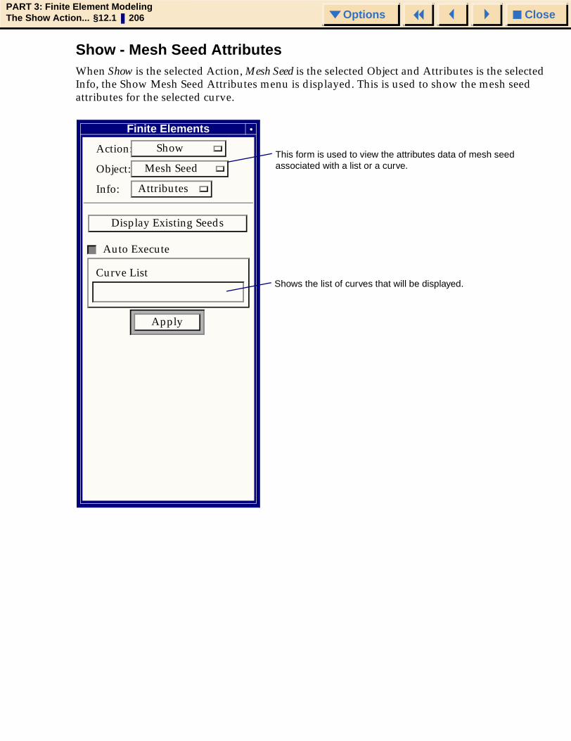
CloseOptionsPART 3: Finite Element ModelingThe Show Action... §12.1 206 Options
Show - Mesh Seed AttributesWhen Show is the selected Action, Mesh Seed is the selected Object and Attributes is the selected Info, the Show Mesh Seed Attributes menu is displayed. This is used to show the mesh seed attributes for the selected curve.
Finite Elements
Action: Show
Object: Mesh Seed
Info: Attributes
Display Existing Seeds
Auto Execute
Curve List
Apply
Shows the list of curves that will be displayed.
This form is used to view the attributes data of mesh seed associated with a list or a curve.

CloseOptionsPART 3: Finite Element ModelingThe Show Action... §12.1 207 Options
Show - Mesh Control AttributesWhen Show is the selected Action, Mesh Control is the selected Object and Attributes is the selected Info, the Show Mesh Control Attributes menu is displayed. This is used to show the mesh control attributes for the selected surfaces.
Finite Elements
Action: Show
Object: Mesh Control
Info: Attributes
Display Existing Seeds
Auto Execute
Surface List
Apply
This form is used to view the attributes data of mesh control on a list of surfaces

CloseOptionsPART 3: Finite Element ModelingThe Show Action... §12.1 208 Options
Show - MPCWhen Show is the selected Action and MPC is the selected Object, the Show MPC form is displayed. Use this to view the attributes of existing MPCs.
Brings up the Show Terms form. This form is used to view the dependent and independent terms.
Indicates the value of the Constant Term, if supported by this MPC type.
Indicates the MPC type currently selected. If the MPC is not valid for the current Analysis Code and Analysis Type preferences, this label will read:
Not Valid for Current PreferencesIn this case, the remaining widgets will not be displayed.
The MPC Summary table lists statistics about the existing MPCs in the database, including the highest ID currently used, the total number of MPCs in the database and the total number of MPCs in the current group.
Finite Elements
Show Action:
MPC Object:
Last ID: 1
Total in Model: 1
Total in ‘default_group’ 1
MPC Summary
MPC ID
MPC Type: Explicit
Constant Term: 0.34
Analysis Preferences:
MSC.Nastran Structural
Indicates the current settings of the Analysis Code and Analysis Type Preferences.
Used to specify the MPC to be shown. The form will be updated automatically whenever the contents of this databox are changed to reflect the attributes of the existing MPC. If the MPC does not exist, the remaining widgets in this form are not displayed.
MPC 1234571
Show Terms...

CloseOptionsPART 3: Finite Element ModelingThe Show Action... §12.1 209 Options
Show - MPC Terms
The Show Terms form appears when the Show Terms button is selected on the Show MPC menu. Use this form to view information about the dependent and independent terms of an MPC.
Show Terms
Dependent Terms (1)
Independent Terms (No Max)
Node 4
Node List
UY
DOFs
Nodes (1) DOFs (1)
Coefficient Nodes (1) DOFs (1)
UX
Coefficient:
2 UX
2.3 3 UY
-4.75 4 UZ
UZ
-4.75 Coefficient Label indicating the value of the coefficient of the selected term, which is displayed only if a term including a coefficient is selected.
A Sequence Label (not shown) indicating the value of the sequence of the selected term is displayed only if a term including a sequence is selected.
Node List textbox indicating the nodes associated to the selected term, which is displayed only if a term is selected.
DOF listbox (read only) indicating the degrees-of-freedom associated with the selected term, which is displayed only if a term including degrees-of-freedom is selected.
Holds the dependent and independent term information as rows in the spreadsheet. A term consists of one or more of the following:
1) A sequence number (not shown)
2) A nonzero coefficient
3) A list of nodes
4) A list of degrees-of-freedom
Terms from these spreadsheets can be selected for an expanded listing of term components.
OK

CloseOptionsPART 3: Finite Element ModelingThe Show Action... §12.1 210 Options
CloseOptionsPART 3: Finite Element ModelingThe Modify Action... § 211 Options
MSC.Patran Reference Manual, Part 3: Finite Element Modeling
CHAPTER
13 The Modify Action
■ Introduction to Modification
■ Modify Forms

CloseOptionsPART 3: Finite Element ModelingThe Modify Action... §13.1 212 Options
13.1 Introduction to ModificationThe purpose of modification is to change one or more attributes of nodes, elements, and or MPCs which have been created, using one of the Create options in the Finite Element application.
Node modify options can affect the ID numbering, location, or the associated analysis and reference coordinate frames of an individual node or a group of nodes.
Element modify options can affect ID numbering, element topology (linear or higher order), or nodal connectivity (manual assignment or reversal of current connectivity).
Bar modify can split a bar element in two.
Tria modify can split a tria element into a pattern of two to four elements.
Quad modify can split a quad element into a pattern of two or four elements or NxM quad elements.
The MPC modify option can be used to add, modify, or delete terms of a currently existing MPC. Attributes of a term that can be modified include the sequence, coefficients, nodes, and the degrees-of-freedom.
Mesh modify, mesh smoothing is an iterative algorithm that can be used to optimize the shape of elements in an existing finite element mesh. Two principle uses for this feature are:
1. To more mesh nodes to the locations of “hard points” and then smooth the modified mesh. Hard points might be the locations of attachments or boundaries of holes.
2. Alter the default setting of a mesh smoothing parameter and then re-smooth the mesh. (Any transition mesh is smoothed automatically when originally created. In most cases, the default parameters yield an acceptable mesh.)
Mesh Seed modify allows the user to modify mesh control from one type to another without having to delete the old one and create a new one in place of the old one. This feature is particularly useful when user needs a node at a certain location when the edge has already been seeded with a certain type.

CloseOptionsPART 3: Finite Element ModelingThe Modify Action... §13.2 213 Options
13.2 Modify FormsWhen Modify is the selected action, the following options are available.
Object Type Description
Mesh Surface Improve an existing surface mesh with optional hard nodes.
Solid Improve an existing solid mesh with optional hard nodes.
Sew Stitches gaps on a mesh.
Mesh Seed Mesh Seed Allows modification of mesh seed on curves/edges.
Element Edit Changes attributes such as ID numbering, element topology, or nodal connectivity of selected elements.
Reverse Reverses the connectivity definition (and therefore the normal direction) of selected elements.
Separate Adds nodes to specified elements an separates them from the rest of the model.
Bar Split Splits a bar element in two.
Tria Split Splits a tria element into two to four elements.
Quad Split Splits a quad element into two to four elements.
Tet Split Splits a tet element.
Node Move Changes a nodal location.
Offset Moves nodes by an indicated vector distance.
Edit Changes attributes such as ID numbering, associated analysis and reference coordinate frames, or physical location of selected nodes.
Project Project nodes onto Surfaces, Curves or a constant coordinate plane (e.g X = 5).
MPC Changes the attributes of a selected MPC.

CloseOptionsPART 3: Finite Element ModelingThe Modify Action... §13.2 214 Options
Modifying MeshThe smoothing algorithm used is the iterative Laplacian-Isoparametric scheme developed by L. R. Herrmann. The final mesh and the execution time for smoothing are controlled by the Smoothing Parameters.
Brings up the Smoothing Parameters form to change smoothing parameter values. These are the same parameters that are used during mesh creation.
Specifies nodes which will remain stationary during smoothing. Nodes around the perimeter of each surface will be treated as hard nodes automatically. This function is optional.
Selects surface(s) to be smoothed. Each surface will be smoothed individually. All elements associated with a surface will be included in the smoothing operation. Elements may have been created by IsoMesh or Paver, or they may have been created or modified by element editing.
Finite Elements
Action: Modify
Object:
Method:
Mesh
Surface
Parameters...
[Hard Node List]
Surface List
-Apply-
Operation: Smoothing

CloseOptionsPART 3: Finite Element ModelingThe Modify Action... §13.2 215 Options
Smoothing Parameters
Figure 13-1
Sets weighting factor for combining Laplacian and Isoparametric smoothing. At the extreme left, pure Laplacian smoothing is used; at the extreme right, pure Isoparametric smoothing is used; at intermediate positions, a combination of the two methods is used. Pure Laplacian smoothing was selected as the default Smoothing Factor because it produces the best mesh in most cases. One notable exception occurs when a surface has significant inplane curvature. In this case, Laplacian smoothing pulls the elements toward edges with inner curvature. Isoparametric smoothing is usually better in this case. See Figure 13-2.
Sets the maximum number of iterations allowed for mesh smoothing. Default value is 20.
If selected, the smoothing parameters will be reset back to the original factory default values. These are: Smoothing Factor = 0.0, Maximum Cycles = 20, Acceleration Factor = 0.00, Termination Factor = 0.05.
If selected, MSC.Patran will reset the smoothing parameter values back to the original set of values that existed upon entry to the Mesh Parameters form.
Sets the smoothing acceleration factor. This factor increases the distance each node is moved during a smoothing cycle and may thus allow smoothing to converge in fewer cycles. For example, a value of 0.5 causes each node to move 50% farther than computed at each iteration. However, caution is advised because this factor can also make the smoothing process diverge, particularly if the geometry is highly curved or skewed. Therefore, a warning is given whenever this factor is set above a value of 0.1.
Controls the smoothing termination tolerance factor. Default value is 0.05, where smoothing stops when the largest distance moved by any node during the previous iteration is less than 5% of the shortest element length along an edge of the geometry.
Smoothing Parameters
Iso Lapl
99 0
1.00 0.00
0.20 0.00
Defaults
Apply Cancel

CloseOptionsPART 3: Finite Element ModelingThe Modify Action... §13.2 216 Options
Figure 13-2 Example Meshes with Different Values of Smoothing Factor
Hybrid Smoothing Isoparametric Smoothing
Laplacian Smoothing Hybrid Smoothing Isoparametric Smoothing
Laplacian Smoothing Hybrid Smoothing Isoparametric Smoothing
Laplacian Smoothing
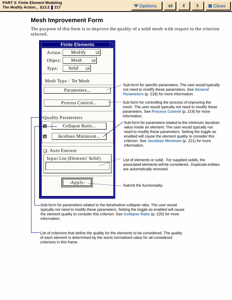
CloseOptionsPART 3: Finite Element ModelingThe Modify Action... §13.2 217 Options
Mesh Improvement FormThe purpose of this form is to improve the quality of a solid mesh with respect to the criterion selected.
Sub-form for specific parameters. The user would typically not need to modify these parameters. See General Parameters (p. 218) for more information.
List of elements or solid. For supplied solids, the associated elements will be considered. Duplicate entities are automatically removed.
Submit the functionality.
Action: Modify
Object: Mesh
Type: Solid
Mesh Type : Tet Mesh
Parameters...
Auto Execute
Input List (Element/Solid)
-Apply-
Finite Elements
Quality Parameters
Collapse Ratio...
Jacobian Minimum...
Sub-form for parameters related to the minimum Jacobian value inside an element. The user would typically not need to modify these parameters. Setting the toggle as enabled will cause the element quality to consider this criterion. See Jacobian Minimum (p. 221) for more information.
Sub-form for parameters related to the tetrahedron collapse ratio. The user would typically not need to modify these parameters. Setting the toggle as enabled will cause the element quality to consider this criterion. See Collapse Ratio (p. 220) for more information.
List of criterions that define the quality for the elements to be considered. The quality of each element is determined by the worst normalized value for all considered criterions in this frame.
Process Control... Sub-form for controlling the process of improving the mesh. The user would typically not need to modify these parameters. See Process Control (p. 219) for more information.

CloseOptionsPART 3: Finite Element ModelingThe Modify Action... §13.2 218 Options
General Parameters
General Parameters
Maintain Element toGeometry Association
[Hard Node List]
Information Output Level
None
Summary
Detailed
Defaults
OK Cancel
List of hard nodes, not to be modified.
Level of information on the bad elements initially in the mesh, during iterations, and those left in the end (if any):
None: Only the percentage of completion forms are displayed while the process is running.
Summary: In addition to information displayed under "None", the history window and session file will indicate the elements failing the criterion in the original state of the mesh, a status line for each iteration, a table of failing elements in the final state of the mesh and some advice if applicable.
Detailed: In addition to information displayed under "Summary", exact references are given for the elements reference in each iteration status line.
Reset default values.
Exit this form without considering changes.
Accept the changes and close this form.
Enabled in order to consider geometric boundaries and create new node/element geometric association. When disabled, the solid mesh will still consider its boundary, but ignore delimitation of the surfaces which define the solids to which the elements may be associated. The later (disabled) is the same as if the envelope of the solid mesh corresponds to a single geometric surface.
Allow Increase
FEM Volume Control
FEM Volume Control for non-snapping element edges on mesh boundary: This only applies for edges on the mesh boundary without an associated geometry of lower order than that of the mesh. Choices are : "Allow Increase", "Allow Decrease", "Constant", "Any Change".
Modifiable Mesh Domain
◆
◆◆
◆
◆◆
◆◆
Complete Mesh
Bad Element Cluster Layers
3
Allows you to specify how many layers around each bad element you want to consider as a modifiable region. Or you can pick all of the mesh.
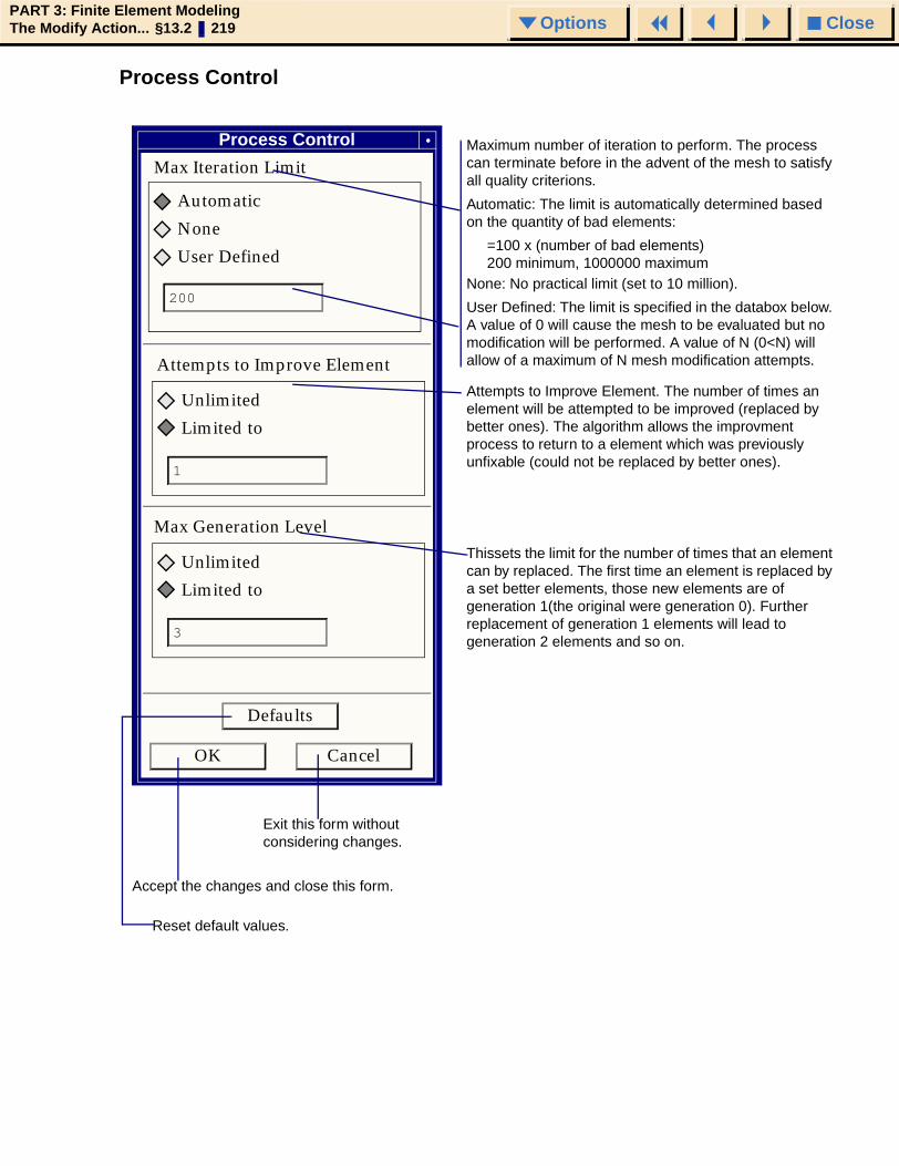
CloseOptionsPART 3: Finite Element ModelingThe Modify Action... §13.2 219 Options
Process Control
Process Control
Max Iteration Limit
Automatic
None
User Defined
200
Defaults
OK Cancel
Maximum number of iteration to perform. The process can terminate before in the advent of the mesh to satisfy all quality criterions.
Automatic: The limit is automatically determined based on the quantity of bad elements:
=100 x (number of bad elements)200 minimum, 1000000 maximum
None: No practical limit (set to 10 million).
User Defined: The limit is specified in the databox below. A value of 0 will cause the mesh to be evaluated but no modification will be performed. A value of N (0<N) will allow of a maximum of N mesh modification attempts.
Reset default values.
Exit this form without considering changes.
Accept the changes and close this form.
Attempts to Improve Element
Max Generation Level
Unlimited
Limited to
1
Unlimited
Limited to
3
Attempts to Improve Element. The number of times an element will be attempted to be improved (replaced by better ones). The algorithm allows the improvment process to return to a element which was previously unfixable (could not be replaced by better ones).
Thissets the limit for the number of times that an element can by replaced. The first time an element is replaced by a set better elements, those new elements are of generation 1(the original were generation 0). Further replacement of generation 1 elements will lead to generation 2 elements and so on.

CloseOptionsPART 3: Finite Element ModelingThe Modify Action... §13.2 220 Options
Collapse Ratio
Collapse Ratio
0.01
Defaults
OK Cancel
Allow Automatic LocalElement Tolerance Ratio
Acceptance Value
Smallest altitudedivided by thelongest edge.
The acceptance value for the selected criterion. This is typically 0.01 for a subsequent NASTRAN analysis. Normalized value will be established from this value and ultimate limits : 0.0 and sqrt(2/3).
When enabled, allows to find another value for the "Local Element Tolearnce Ratio" for individual element which can not be improved with the value supplied. It is recommended to always enable this option.
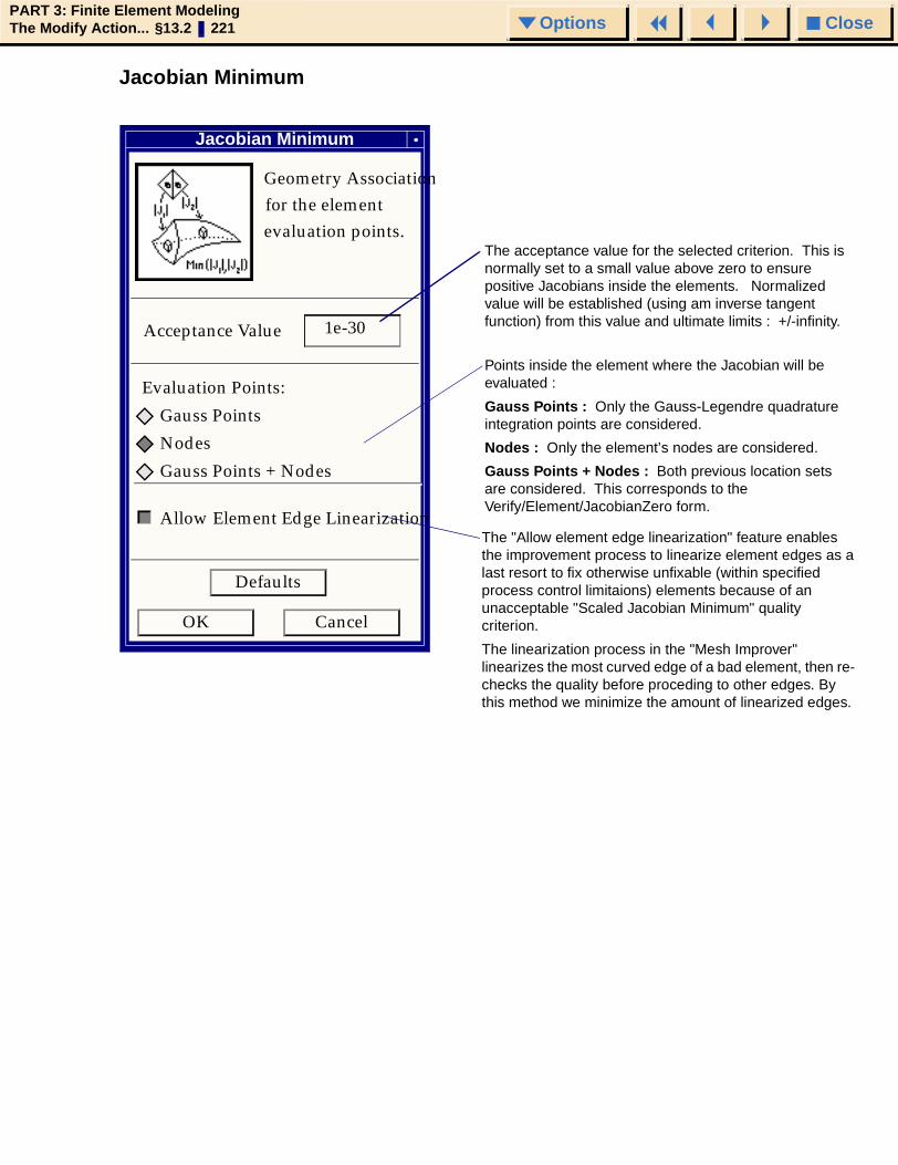
CloseOptionsPART 3: Finite Element ModelingThe Modify Action... §13.2 221 Options
Jacobian Minimum
Jacobian Minimum
Geometry Association
Acceptance Value
Evaluation Points:
Gauss Points
Nodes
Gauss Points + Nodes
Defaults
OK Cancel
1e-30
for the element evaluation points.
The acceptance value for the selected criterion. This is normally set to a small value above zero to ensure positive Jacobians inside the elements. Normalized value will be established (using am inverse tangent function) from this value and ultimate limits : +/-infinity.
Points inside the element where the Jacobian will be evaluated :
Gauss Points : Only the Gauss-Legendre quadrature integration points are considered.
Nodes : Only the element’s nodes are considered.
Gauss Points + Nodes : Both previous location sets are considered. This corresponds to the Verify/Element/JacobianZero form.
Allow Element Edge LinearizationThe "Allow element edge linearization" feature enables the improvement process to linearize element edges as a last resort to fix otherwise unfixable (within specified process control limitaions) elements because of an unacceptable "Scaled Jacobian Minimum" quality criterion.
The linearization process in the "Mesh Improver" linearizes the most curved edge of a bad element, then re- checks the quality before proceding to other edges. By this method we minimize the amount of linearized edges.

CloseOptionsPART 3: Finite Element ModelingThe Modify Action... §13.2 222 Options
Modifying Mesh SeedThe modify mesh seed menu allows users to change mesh seed types.
Finite Elements
Action: Modify
Object: Mesh Seed
Display Existing Seeds
Auto Show Seed Data
Select One Curve
Show Seeds Data
New Mesh Seed InfoType Uniform
Element Edge Length Data
Number of Elements
Number = 2
-Apply-
L
◆
Select the curve for which mesh seed needs to be modified.
Click here to show the seed data. Use this to fill the tabular seed locations if the table has been Cleared. Under normal circumstances it can be used to display the mesh seed information table.
The options available are Uniform, One Way, Two Way and Tabular mesh seed types.

CloseOptionsPART 3: Finite Element ModelingThe Modify Action... §13.2 223 Options
Sew FormUsing Modify/Mesh/Sew form sews gaps on a mesh consisting of all tria3 elements. This program removes interior free edges on a mesh by merging nodes and splitting triangles automatically (see Figure 13-3 and Figure 13-4).
Figure 13-3 Mesh Before Sewing
Figure 13-4 Mesh After Sewing

CloseOptionsPART 3: Finite Element ModelingThe Modify Action... §13.2 224 Options
The primary purpose of this program is to provide users a useful tool to obtain a congruent mesh which will be used to create a tessellated surface. (See Created Tessellated Surface from Geometry Form (p. 306) in the MSC.Patran Reference Manual, Part 2: Geometry Modeling.) For this reason, the elements modified or created by this program may not have very good quality.
Finite Elements
Action: Modify
Object: Mesh
Type: Sew
Target Element Edge Length
0.1
Tria Element List
-Apply-
Elm 1:100
Specify a set of tria elements consisting of the mesh to be sewed.
Specify the target element edge length which was used as a global edge length when creating the mesh. The gap tolerance is equal to one tenth of the target element length.

CloseOptionsPART 3: Finite Element ModelingThe Modify Action... §13.2 225 Options
Modifying Elements
Edit Method
When one of these attributes is selected, the appropriate information to modify appears on the form. When this form is initially opened, none of the attributes are selected; therefore, only the Element Attributes toggle is initially displayed. Any combination of these attributes may be selected. If only Connectivity is selected, a toggle will become visible to modify all elements associated to the current nodelist.
For information regarding this toggle see Output ID List (p. 25) in the MSC.Patran Reference Manual, Part 1: Basic Functions.
Lists the nodes to be modified for each element.
This box appears on the form when any element attribute is selected. It lists the ID numbers of the elements to which the changes apply.
Specifies shape of the new elements.
Specifies topology of the new elements.
The list of nodes which are to replace those in the Current Node List. There is a one-to-one correspondence between the Current Node List and the New Node List. In the example shown, Nodes 5 and 7 are to be swapped in the connectivity order for Element 3.
Finite Elements
Action: Modify
Object:
Object:
Object:
Object: Object:
: Element
Method: Edit
Element Attributes
ID
Type
Connectivity
New ID's
Shape Quad
New Topology:
Quad4 Quad5 Quad8 Quad9 Quad12 Quad16
Auto Execute
Element List
Current Node List
New Node List
-Apply-
Elm 3
Node 7 5
Node 5 7

CloseOptionsPART 3: Finite Element ModelingThe Modify Action... §13.2 226 Options
Reverse Method
Specifies the list of elements whose connectivity, and therefore normal direction, is to be reversed.
Finite Elements Action: Modify
Object:
Element
Method: Reverse
Auto Execute
Element List
-Apply-

CloseOptionsPART 3: Finite Element ModelingThe Modify Action... §13.2 227 Options
Separate Method
Specifies the list of elements to be separated.
Specifies the list of nodes. For each node a new node will be created and the element connectivity will be updated for the specified elements. The Node list box will only be visible for option At Nodes. For all other options the nodes associated to the specified entities will be used instead.
The following options are available:
At Nodes: separate elements at nodes
At Elem Edges: separate elements at edges
At Elem Faces: separate elements at faces
At Free Edges: separate elements at free edges
At Free Faces: separate elements at free faces
Toggle to specify if the new nodes will keep the same association to geometry as the old ones.
Finite Elements
Action: Modify
Object:
Element
Method: Separate
Option: At Nodes
Keep Node Association
Auto Execute
Node List
-Apply-
Element list

CloseOptionsPART 3: Finite Element ModelingThe Modify Action... §13.2 228 Options
Modifying Bars
Specifies the list of bar elements to split.
Note: The new bars will have the same topology as the parent (i.e., a Bar3 will be split into two Bar3s).
Finite Elements
Action: Modify
Object: Bar
Method: Split
Auto Execute
Bar Element List
-Apply-
1 2 3

CloseOptionsPART 3: Finite Element ModelingThe Modify Action... §13.2 229 Options
Modifying Trias
Splitting a Tria into Two Trias
Select this icon to enable the two tria option.
Selects a position on an edge.
Specify the trias to be split by selecting from the graphics window or entering a list of elements.
Specify the node where the split is to occur. This list may contain one entry for each element or a single entry. If a single entry, each element will be split at the same corner relative to the element origin as the first element.
Note: The new trias will have the same topology as the parent (i.e., a Tria6 will be split into two Tria6s).
Finite Elements
Action: Modify
Object:
Method:
Tria
Split
Replacement Pattern
Auto Execute
Tria Element List
-Apply-
Node List
Split on longest edge
Split at selected node ◆
◆◆
At posn on selected edge◆◆
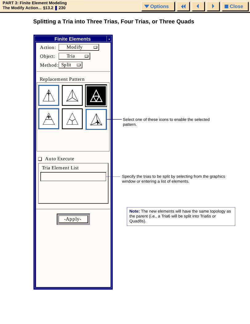
CloseOptionsPART 3: Finite Element ModelingThe Modify Action... §13.2 230 Options
Splitting a Tria into Three Trias, Four Trias, or Three Quads
Select one of these icons to enable the selected pattern.
Specify the trias to be split by selecting from the graphics window or entering a list of elements.
Note: The new elements will have the same topology as the parent (i.e., a Tria6 will be split into Tria6s or Quad8s).
Finite Elements
Action: Modify
Object:
Tria
Method: Split
Replacement Pattern
Auto Execute
Tria Element List
-Apply-

CloseOptionsPART 3: Finite Element ModelingThe Modify Action... §13.2 231 Options
Splitting a Tria into a Tria and a Quad
Select this icon to enable the tria-quad option.
Specify the node to orient the split. This list may contain one entry for each element or a single entry. If a single entry, each element split will be oriented the same relative to the element origin as the first element.
Specify the trias to be split by selecting from the graphics window or entering a list of elements.
Select automatic or manual operation.
Note: The new elements will have the same topology as the parent (i.e., a Tria6 will be split into a Tria6 and a Quad8).
Finite Elements
Action: Modify
Object:
Tria
Method: Split
Replacement Pattern
Auto Execute
Tria Element List
-Apply-
Node List
Tria at sharpest corner
Tria at selected node ◆
◆◆

CloseOptionsPART 3: Finite Element ModelingThe Modify Action... §13.2 232 Options
Splitting Tet Elements
Split a tet element at a selected edge.
Select the edge split location. This list may contain one entry for each element or a single entry. If a single entry, each element split will be oriented the same relative to the element origin as the first element.
Select the tet edge to split.
Split a tet element at a selected face location.
Finite Elements
Action: Modify
Object:
Tet
Method: Split
Replacement Pattern
Auto Execute
Single Element Edge
-Apply-
Split Location (Straight Edge) :
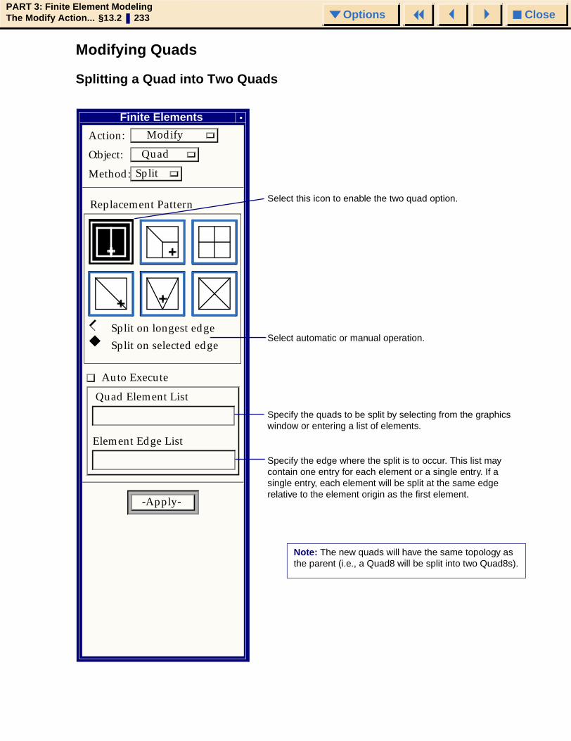
CloseOptionsPART 3: Finite Element ModelingThe Modify Action... §13.2 233 Options
Modifying Quads
Splitting a Quad into Two Quads
Select this icon to enable the two quad option.
Specify the edge where the split is to occur. This list may contain one entry for each element or a single entry. If a single entry, each element will be split at the same edge relative to the element origin as the first element.
Specify the quads to be split by selecting from the graphics window or entering a list of elements.
Select automatic or manual operation.
Note: The new quads will have the same topology as the parent (i.e., a Quad8 will be split into two Quad8s).
Finite Elements
Action: Modify
Object:
: Quad
Method: Split
Replacement Pattern
Auto Execute
Quad Element List
-Apply-
Split on longest edge
Split on selected edge
Element Edge List
◆
◆◆

CloseOptionsPART 3: Finite Element ModelingThe Modify Action... §13.2 234 Options
Splitting a Quad into Three Quads
Select this icon to enable the three quad option.
Specify the quads to be split by selecting from the graphics window or entering a list of elements.
Note: The new quads will have the same topology as the parent (i.e., a Quad8 will be split into three Quad8s).
Specify the node to orient the split. This list may contain one entry for each element or a single entry. If a single entry, each element split will be oriented the same relative to the element origin as the first element.
Finite Elements
Action: Modify
Object: Quad
Method: Split
Replacement Pattern
Auto Execute
Quad Element List
-Apply-
Node List

CloseOptionsPART 3: Finite Element ModelingThe Modify Action... §13.2 235 Options
Splitting a Quad into Four Quads or Four Trias or NxM Quads
Figure 13-5
Select one of these icons to enable the selected pattern.
Specify the quads to be split by selecting from the graphics window or entering a list of elements.
Note: The new elements will have the same topology as the parent (i.e., a Quad8 will be split into Quad8s or Tria6s).
Specify the edge where the split is to occur. This list may contain one entry for each element or a single entry. If a single entry, each element will be split at the same edge.
Specify the number of elements to be created at the two edge directions. N specifies the number of elements at the selected edge, M the other direction. This method will split all elements with the same pattern, unless they are not connected and no shared edges can be found.
Option for a 2 x 2 or n x m split only available for quad elements.
Finite Elements
Action: Modify
Method:
Object: Quad
Split
Replacement Pattern
Split in 2 x 2 Quads
Split in N x M Quads
Auto Execute
Quad Element List
Element Edge List
Specify N,M: N at selected Edge
N 2
M 2
-Apply-
◆
◆◆

CloseOptionsPART 3: Finite Element ModelingThe Modify Action... §13.2 236 Options
Splitting a Quad into Two Trias
Figure 13-6
Select this icon to enable the two tria option.
Specify the node where the split is to occur. This list may contain one entry for each element or a single entry. If a single entry, each element will be split at the same corner relative to the element origin as the first element.
Specify the quads to be split by selecting from the graphics window or entering a list of elements.
Select automatic or manual operation.
Note: The new trias will have the same topology as the parent (i.e., a Quad8 will be split into two Tria6s).
Finite Elements
Action: Modify
Object:
: Quad
Method: Split
Replacement Pattern
Auto Execute
Quad Element List
Node List
-Apply-
Split on shorter diagonal
Split at selected node ◆
◆◆

CloseOptionsPART 3: Finite Element ModelingThe Modify Action... §13.2 237 Options
Splitting a Quad into Three Trias
Figure 13-7
Select this icon to enable the three tria option.
Specify the quads to be split by selecting from the graphics window or entering a list of elements.
Note: The new trias will have the same topology as the parent (i.e., a Quad8 will be split into three Tria6s).
Specify the edge to orient the split. This list may contain one entry for each element or a single entry. If a single entry, each element split will be oriented the same relative to the element origin as the first element.
Finite Elements
Action: Modify
Object:
Method:
: Quad
Split
Replacement Pattern
Auto Execute
Quad Element List
Element Edge List
-Apply-

CloseOptionsPART 3: Finite Element ModelingThe Modify Action... §13.2 238 Options
Modifying Nodes
Move Method
Figure 13-8
Specifies a list of new node locations by entering coordinates in the global rectangular system (as shown) or by using the select menu.
Specifies the list of nodes to be moved.
Finite Elements
Action: Modify
Object:
: Node
Method: Move
Auto Execute
Node List
Node 101 102
New Node Locations
[0 12.5 o] [0 13.2 .5]
-Apply-
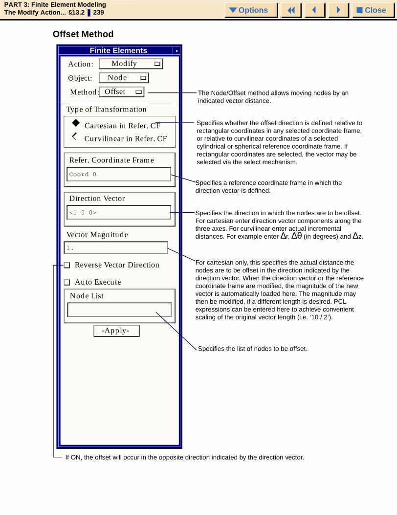
CloseOptionsPART 3: Finite Element ModelingThe Modify Action... §13.2 239 Options
Offset Method
Specifies a reference coordinate frame in which the direction vector is defined.
Specifies the list of nodes to be offset.
If ON, the offset will occur in the opposite direction indicated by the direction vector.
The Node/Offset method allows moving nodes by an indicated vector distance.
Specifies whether the offset direction is defined relative to rectangular coordinates in any selected coordinate frame, or relative to curvilinear coordinates of a selected cylindrical or spherical reference coordinate frame. If rectangular coordinates are selected, the vector may be selected via the select mechanism.
Specifies the direction in which the nodes are to be offset. For cartesian enter direction vector components along the three axes. For curvilinear enter actual incremental distances. For example enter ∆r, ∆θ (in degrees) and ∆z.
For cartesian only, this specifies the actual distance the nodes are to be offset in the direction indicated by the direction vector. When the direction vector or the reference coordinate frame are modified, the magnitude of the new vector is automatically loaded here. The magnitude may then be modified, if a different length is desired. PCL expressions can be entered here to achieve convenient scaling of the original vector length (i.e. ‘10 / 2‘).
Finite Elements
Action: Modify
Object:
Method:
: Node
Offset
Type of Transformation
Cartesian in Refer. CF
Curvilinear in Refer. CF
Refer. Coordinate Frame
Coord 0
Direction Vector
<1 0 0>
Vector Magnitude
1.
Reverse Vector Direction
Auto Execute
Node List
-Apply-
◆◆
◆

CloseOptionsPART 3: Finite Element ModelingThe Modify Action... §13.2 240 Options
Edit Method
New physical location(s) of the listed node(s). Enter coordinates in the global rectangular system or use the select menu.
Used to input new node ID numbers for the listed nodes. See Output ID List (p. 25) in the MSC.Patran Reference Manual, Part 1: Basic Functions.
ID number of a coordinate frame where the displacements, degrees-of-freedom, constraints, and solution vectors are defined for the listed nodes.
Appears when any nodal attribute is selected. It lists the ID numbers of the nodes which are to be changed.
When one of these attributes is selected, the appropriate information to modify appears on the form. When this form is initially opened, none of the attributes are selected, therefore, only the Nodal Attributes box is displayed.
ID number of a coordinate frame where the location is defined for the listed nodes.
Finite Elements
Action: Modify
Object:
Method:
Node
Edit
Nodal Attributes
ID Analysis Coordinate Frame Refer. Coordinate Frame Location
New Node ID's
Analysis Coordinate Frame
Refer. Coordinate Frame
Node Locations
Auto Execute
Node List
-Apply-

CloseOptionsPART 3: Finite Element ModelingThe Modify Action... §13.2 241 Options
Project Method
Closest to Surf option will project the existing nodes by using the closest approach to the specified surface or face.
Define Vector option allows you to specify the coordinates of the Projection Vector and the Refer. Coordinate Frame to express the vector within. (Example: <1 1 0>). The Vector select menu will appear to allow you alternate ways to cursor define the vector direction.
View Vector option will project the existing points by using the view angle of the current viewport. MSC.Patran will project the existing nodes using the normal direction of the screen.
Closest to Curve option will project the existing nodes by using the closest approach to the specified curve or edge.
To Plane option will project the existing nodes by changing the selected coordinate value in a specified reference coordinate system.
Projection Vector and Refer. Coordinate Frame is used if the Define Vector option is chosen.
Select Nodes to be projected with the selected option.
Specify Surfaces or Curves that the nodes will be projected onto.
Finite Elements
Action: Modify
Object:
Method:
Object: Node
Project
Option: Closest to Surf
Auto Execute
Input Nodes
Surface List
-Apply-
Projection Vector
<0 0 0>
Refer. Coordinate Frame
Coord 0

CloseOptionsPART 3: Finite Element ModelingThe Modify Action... §13.2 242 Options
Modifying MPCsWhen Modify is the selected Action and MPC is the selected Object, the Modify MPC form is displayed. Use this form to modify the attributes of existing MPCs.
Brings up the Modify Terms form. Use to create, modify or delete dependent and independent terms.
Specifies a constant term, if supported by the current selected MPC type.
Indicates the MPC type currently selected. If the MPC is not valid for the current Analysis Code and Analysis Type preferences, this label will read:
Not Valid for Current Preferences
In this case, the remaining widgets will not be displayed.
Indicates the current settings of the Analysis Code and Analysis Type Preferences.
Used to specify the MPC to be modified. The form will be updated automatically whenever the contents of this databox are changed to reflect the attributes of the existing MPC. If the MPC does not exist, the remaining widgets in this form are not displayed.
Finite Elements
Action: Modify
Object:
: MPC
Analysis Preferences: :ANSYS Structural
MPC ID
MPC 1234571
MPC Type:
0
Constant
Modify Terms...
-Apply- Reset
Explicit

CloseOptionsPART 3: Finite Element ModelingThe Modify Action... §13.2 243 Options
Modify Terms
This form appears when the Modify Terms button is selected on the Modify MPC form. Use this form to modify the dependent and independent terms of a selected MPC.
Modify Terms
Create Dependent
Create Independent
Modify
Delete
Node 101,109:124:5
Node List
Auto Execute
DOFs
Dependent Terms (1)
Nodes (1) DOFs (1 )
101,109:124:5 UX,UY,UZ
Independent Terms (No Max)
Coefficient Nodes (1) DOFs (1)
0.5 5:25:5 UX,UY,UZ
UX UYUZ
Sets the mode of the Apply function to:
1. Create a dependent term.2. Create an independent term.3. Modify a term, or4. Delete a term. The Create Dependent and Create Independent items are disabled once the maximum number of dependent or independent terms are created.
Specifies a nonzero coefficient for a term. This widget is displayed when creating or modifying a term which includes a Coefficient column.
Specifies the nodes for a term. This widget is displayed when creating or modifying a term which includes a Nodes column.
Select the degrees-of-freedom for a term. This widget is displayed when creating or modifying a term, which includes a DOFs column.
Holds the dependent and independent term information as rows in the spreadsheet. The number of terms required is displayed in parentheses next to the spreadsheet label. A term consists of one or more of the following:
1. A sequencer number (not shown).2. A nonzero coefficient.3. A list of nodes (the required number is
displayed in parentheses).4. A list of degrees-of-freedom (the required
number is listed in parentheses).Existing terms can be selected for modification and deletion.
0.5Coefficient =
-Apply- Clear Cancel
◆◆
◆◆ ◆◆
◆
UY

CloseOptionsPART 3: Finite Element ModelingThe Modify Action... §13.2 244 Options

CloseOptionsPART 3: Finite Element ModelingThe Delete Action... § 245 Options
MSC.Patran Reference Manual, Part 3: Finite Element Modeling
CHAPTER
14 The Delete Action
■ Delete Action
■ Delete Forms

CloseOptionsPART 3: Finite Element ModelingThe Delete Action... §14.1 246 Options
14.1 Delete ActionThe Delete action provides the capability to remove finite element entities from the model database. Submenus are provided to selectively delete any combination of finite element entities or specifically Node, Element, Mesh Seed definitions, Mesh on Curve ⁄Surface ⁄Solid, or MPC entities. By default, Auto Execute is selected which means MSC.Patran will automatically delete after the entities are selected.
If there are many finite element entities to be deleted, a percent complete form will show the status of the delete process for each entity type. When deletion is complete, a report appears in the command line indicating the number and IDs of the entities deleted, and the number and IDs of the entities not found and therefore not deleted.
The association of the deleted entity with other related entities is broken during deletion. Nodes, element properties, loads and boundary conditions, results and groups may become unreferenced due to deletion. Toggles are provided to delete unreferenced nodes and empty groups due to the delete function. The current group will not be deleted even if it becomes empty.
The Abort key may be selected at any time to halt the delete process, and the Undo button may be used to restore the deleted entities.

CloseOptionsPART 3: Finite Element ModelingThe Delete Action... §14.2 247 Options
14.2 Delete FormsWhen Delete is the selected action, the following options are available.
Object Type Description
Any Allows for deletion of multiple types of finite element entities at once. Related nodes, element properties, load and boundary conditions, results and groups may become unreferenced due to deletion.
Mesh Seed Deletes the mesh seed definitions from the specified edges.
Mesh Control Deletes the mesh control applied to a surface.
Mesh Surface Deletes the mesh from the specified surfaces.
Curve Deletes the mesh from the specified curves.
Solid Deletes the mesh from the specified solids.
Node Deletes the specified nodes. Element corner nodes will not be deleted. Related load and boundary conditions, results are disassociated with the deleted nodes but they are not deleted. Any nodes associated with a DOF list will be removed from the nodes portion of the DOF list term. A toggle is provided to delete empty groups due to the deletion.
Element Deletes the specified elements. Nodes, element properties, load and boundary conditions, results and groups are disassociated with the deleted elements but they are not deleted. A toggle is provided to delete related nodes and empty groups due to the deletion.
MPC Deletes the multi-point constraints. Nodes and groups are disassociated with the deleted MPCs but they are not deleted. A toggle is provided to delete related nodes and empty groups due to the deletion.
Superelement Deletes the superelements.
DOF List Deletes the specified degree-of-freedom (DOF) lists.

CloseOptionsPART 3: Finite Element ModelingThe Delete Action... §14.2 248 Options
Delete - Any Use this form to delete multiple types of finite element entities at one time. Any combination of elements, nodes, and multi-point constraints may be selected for deletion. When deleting elements and nodes, the mesh on curves, surfaces and solids may also be deleted. However, mesh seeds can only be deleted through the Delete/Mesh Seed menu. Nodes, element properties, loads and boundary conditions, results and groups may become unreferenced due to deletion. Toggles are provided to delete unreferenced nodes and empty groups due to the delete operation.
Selects and displays the entity types which can be selected for deletion from the viewport.
Specifies the list of finite element entities to be deleted. Either cursor select, type in the entity types and IDs, or by using the Finite Element select menu.
Specifies the entity types to be deleted. Set the appropriate toggles ON or OFF.
Specifies Nodes which are selectable for deletion (default is ON). Empty Groups – Set toggle ON to indicate groups have become empty due to the deletion of nodes.
Specifies Elements are selectable for deletion (default is ON). Node – Deletes all nodes that are related to the deleted elements (default is ON). Empty Groups – Set toggle ON (default OFF) to indicate groups have become empty due to deletion of elements.
By default, Auto Execute is OFF. This means MSC.Patran will not automatically delete after the objects are selected.
Specifies MPCs are selectable for deletion (default is OFF). Node– Deletes all nodes which are related to the deleted MPCs. Empty Groups – Toggle ON to indicate that groups that become empty due to the deletion of MPCs should be deleted.
Finite Elements
Action: Delete
Object: Any
Delete Node and Related
Empty Groups Element and Related
Node Empty Groups
MPC's Node Empty Groups
Auto Execute Finite Element Entity List Node 1:900 Element 5:20
-Apply-
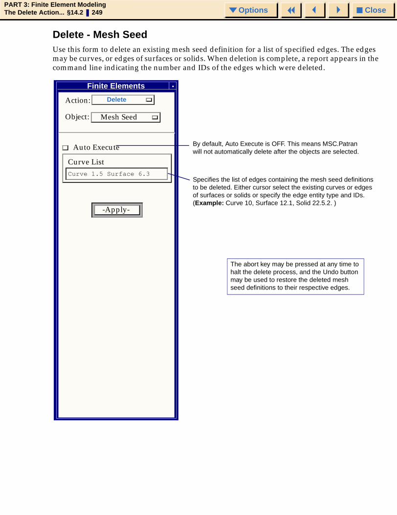
CloseOptionsPART 3: Finite Element ModelingThe Delete Action... §14.2 249 Options
Delete - Mesh SeedUse this form to delete an existing mesh seed definition for a list of specified edges. The edges may be curves, or edges of surfaces or solids. When deletion is complete, a report appears in the command line indicating the number and IDs of the edges which were deleted.
Specifies the list of edges containing the mesh seed definitions to be deleted. Either cursor select the existing curves or edges of surfaces or solids or specify the edge entity type and IDs. (Example: Curve 10, Surface 12.1, Solid 22.5.2. )
By default, Auto Execute is OFF. This means MSC.Patran will not automatically delete after the objects are selected.
The abort key may be pressed at any time to halt the delete process, and the Undo button may be used to restore the deleted mesh seed definitions to their respective edges.
Finite Elements
Action:
Object: Mesh Seed
Auto Execute
Curve List Curve 1.5 Surface 6.3
-Apply-
Delete

CloseOptionsPART 3: Finite Element ModelingThe Delete Action... §14.2 250 Options
Delete - Mesh (Surface)Use this form to delete an existing mesh of nodes and elements applied to one or more surfaces, or solid faces. When deletion is complete, a report appears in the command line indicating the number and IDs of the entities from which meshes were deleted.
Specifies the list of geometric entities that are meshed by cursor or by entering the entity type and IDs. (Example, to delete a mesh from a Surface enter: Surface 12, Solid 22.4.)
Types which can be selected are: Curve, Surface, or Solid.
By default, Auto Execute is OFF. This means MSC.Patran will not automatically delete after the objects are selected.
The abort key may be pressed at any time to halt the delete process, and the Undo button may be used to restore the deleted mesh of nodes and elements.
Finite Elements
Action: Delete
Object: Mesh
Type: Surface
Auto Execute
Surface List
-Apply-
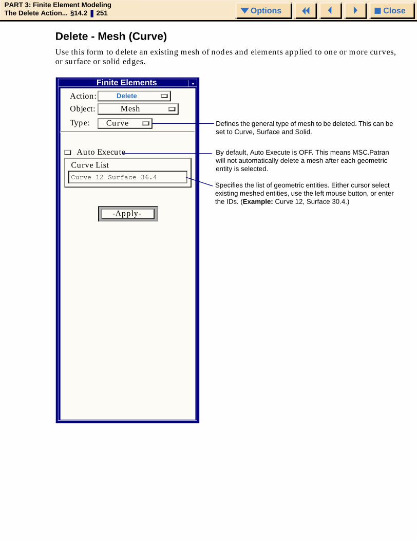
CloseOptionsPART 3: Finite Element ModelingThe Delete Action... §14.2 251 Options
Delete - Mesh (Curve)Use this form to delete an existing mesh of nodes and elements applied to one or more curves, or surface or solid edges.
By default, Auto Execute is OFF. This means MSC.Patran will not automatically delete a mesh after each geometric entity is selected.
Specifies the list of geometric entities. Either cursor select existing meshed entities, use the left mouse button, or enter the IDs. (Example: Curve 12, Surface 30.4.)
Defines the general type of mesh to be deleted. This can be set to Curve, Surface and Solid.
Finite Elements
Action: Delete
Object:
Type:
Mesh
Curve
Auto Execute
Curve List Curve 12 Surface 36.4
-Apply-

CloseOptionsPART 3: Finite Element ModelingThe Delete Action... §14.2 252 Options
Delete - Mesh (Solid)Use this form to delete an existing mesh of nodes and elements applied to one or more solids.
By default, Auto Execute is OFF. This means MSC.Patran will not automatically delete a mesh after each geometric entity is selected.
Specifies the list of geometric entities. Either cursor select existing meshed entities, use the left mouse button, or enter the IDs. (Example: Solid 22.)
Defines the general type of mesh to be deleted. This can be set to Curve, Surface and Solid.
Finite Elements
Action: Delete
Object:
Type:
Mesh
Solid
Auto Execute
Solid List Solid 22
-Apply-

CloseOptionsPART 3: Finite Element ModelingThe Delete Action... §14.2 253 Options
Delete - Mesh Control
Finite Elements
Action: Delete
Object: Mesh Control
Auto Execute
Surface List
-Apply-
List of surfaces from which mesh control should be deleted.

CloseOptionsPART 3: Finite Element ModelingThe Delete Action... §14.2 254 Options
Delete - NodeUse this form to delete existing nodes from the model database. Element corner nodes will not be deleted. Related loads and boundary conditions, results and groups are disassociated with the deleted nodes but they are not deleted. Any nodes associated with a DOF list will be removed from the nodes portion of the DOF list term. A toggle is provided to delete groups that become empty due to the deletion of the nodes. When deletion is complete a report appears in the command line indicating the number and IDs of the nodes deleted.
Allows Empty Groups to be deleted with the node, or left in place. The current group will not be deleted even if it becomes empty.
Specifies the list of nodes which are to be deleted. Select with cursor, or specify node IDs.
Toggle ON to indicate groups which have become empty due to the deletion of nodes, and should be deleted.
By default, Auto Execute is OFF. This means that MSC.Patran will not automatically delete after the objects are selected.
The abort key may be pressed at any time to halt the delete process and the Undo button may be used to restore the deleted nodes and groups.
Finite Elements
Action: Delete
Object:
Node
Delete Related
Empty Groups
Auto Execute
Node List Node 1:1000 1009 1010
-Apply-

CloseOptionsPART 3: Finite Element ModelingThe Delete Action... §14.2 255 Options
Delete - ElementUse this form to delete existing elements from the model database. Related nodes, element properties, loads and boundary conditions, results and groups are disassociated from the deleted elements, but they are not deleted. A toggle is provided to delete all related nodes and empty groups due to the deletion of elements.
Allows for the related nodes and Empty groups to be deleted with the element or left alone. The current group will not be deleted even if it becomes empty.
Specifies the list of elements. Either cursor select, or specifies element IDs. Through the element select menu, elements may be deleted by type (for instance only bar elements or triangular elements... etc.).
Deletes all nodes that are related to the elements which have been deleted (default is ON).
Toggle ON to indicate groups which have become empty due to the deletion of elements, and should be deleted.
By default, Auto Execute is OFF. This means that MSC.Patran will not automatically delete after the objects are selected.
The abort key may be pressed at any time to halt the delete process, and the Undo button may be used to restore the deleted elements and related nodes and groups.
Finite Elements
Action: Delete
Object:
Element
Delete Related
Nodes
Empty Groups
Auto Execute
Element List
Element 2 6 7:65
-Apply-

CloseOptionsPART 3: Finite Element ModelingThe Delete Action... §14.2 256 Options
Delete - MPCUse this form to delete an existing multi-point constraint (MPC) from the database. Related nodes and groups are disassociated from the deleted MPCs, but they are not deleted. A toggle is provided to delete all related nodes and empty groups due to the deletion of the MPCs.
Allows the related nodes and empty groups to be deleted or left in place.
Specifies the list of MPCs to be deleted. Select with the cursor or type in the MPC IDs.
By default, Auto Execute is OFF. This means that MSC.Patran will not automatically delete after the objects are selected.
Deletes all nodes which are related to the MPCs that have been deleted (default is ON).
Toggle ON to indicate groups which have become empty due to the deletion of MPCs and should be deleted.
The abort key may be selected at any time to halt the delete process, and the Undo button may be used to restore the deleted MPCs and related nodes and groups.
Finite Elements
Action: Delete
Object:
MPC
Delete Related
Nodes
Empty Groups
Auto Execute
List of MPC's MPC 1:10 12 15
-Apply-

CloseOptionsPART 3: Finite Element ModelingThe Delete Action... §14.2 257 Options
Delete - SuperelementUse this form to delete superelements from the database. Note that this is currently available only for the MSC.Nastran analysis preference.
List of existing superelements. Only the highlighted superelements are deleted.
Finite Elements
Action: Delete
Object:
Superelement
Superelement List
-Apply-

CloseOptionsPART 3: Finite Element ModelingThe Delete Action... §14.2 258 Options
Delete - DOF ListUse this form to delete degree-of-freedom (DOF) lists from the database. Note that this is currently available only for the ANSYS and ANSYS 5 analysis preference.
Displays a list of all DOF lists currently defined in the database. Highlighting one or more entries and selecting Apply will delete the highlighted DOF lists from the database.
Finite Elements
Action: Delete
Object:
DOF List
Analysis Preferences: Code: ANSYS Type: Structural
Available DOF Lists
-Apply-

CloseOptionsPART 3: Finite Element ModelingThe MSC.Patran Element Library § 259 Options
MSC.Patran Reference Manual, Part 3: Finite Element Modeling
CHAPTER
15 The MSC.Patran Element Library
■ Introduction
■ Beam Element Topology
■ Tria Element Topology
■ Quad Element Topology
■ Tetrahedral Element Topology
■ Wedge Element Topology
■ Hex Element Topology
■ MSC.Patran’s Element Library

CloseOptionsPART 3: Finite Element ModelingThe MSC.Patran Element Library §15.1 260 Options
15.1 IntroductionThe MSC.Patran template database file, template.db, contains a “generic” set of finite element topologies. By default, when opening a new database, the element topology library is included. Topology, in the context of a finite element, is the relative node, edge and face numbering scheme for each element of the same topology. The MSC.Patran library is compatible with earlier versions of MSC.Patran (PATRAN Release 2.5). MSC.Patran also provides additional information about each element topology which was not available in the earlier MSC.Patran versions:
• Nodal parametric locations
• Edge numbering
• Face numbering
• Face sense
• Corresponding degenerate element topology ID
Where possible, the ISO 10303-104, Application Resources: Finite Element Analysis document, which is part of International Standard ISO 10303-Product Data Representation and Exchange (STEP), was used to define the element topologies. If the ISO standard was found to be in conflict with earlier versions of MSC.Patran, the MSC.Patran convention took precedence. The ISO standard for numbering edges and faces of elements is used.
Face and edge numbering are important for assigning element attributes, such as pressures applied to a solid element face. In MSC.Patran, you may select an edge or a face of an element with the cursor. An example of the syntax, used in the Select Databox to describe an edge of hex element 1, would be elem 1.2.3, which refers to edge 3 of face 2 of element 1.
The element topology tables listed in sections 13.2 through 13.7 are used to construct and interpret the syntax of the Select Databox string. MSC.Patran’s Element Library (p. 320) provides illustrations of each element type and topology, and their node locations.
Parametric coordinate systems
Rectangular. [Xi/Eta/Zeta] is used for Tet/Wedge/Hex elements. Values can either have a range of -1 to 1 or 0 to 1 depending on the case where an area or volume coordinate systems can apply (Tet/Wedge elements). [Xi/Eta] applies to a Tri or Quad element. Values range from 0 to 1 for the Tri, and -1 to 1 for the Quad. [Xi] applies to a Bar element. Values range from -1 to 1.
Area. [L1/L2/L3] is used for locating a point within a triangular area. Values range from 0 to 1, and the sum of all cordinates is equal to 1. The values correspond to the weighting with respect to the 3 corners of a triangle. For a Tri or Wedge element which will use [Xi/Eta] and [Xi/Eta/Zeta], the Xi/Eta value will range from 0 to 1, and we can determine L1/L2/L3 as :
L1 = 1.0 - Xi - Eta
L2 = Xi
L3 = Eta
Important: The face sense is interpreted as positive if the normal is pointing away from (towards the outside) the element, using the right hand rule. This only applies to volume elements (element dimensionality = 3).

CloseOptionsPART 3: Finite Element ModelingThe MSC.Patran Element Library §15.1 261 Options
Volume. [L1/L2/L3/L4] is used for locating a point within a tetrahedral volume. Values range from 0 to 1, and the sum of all cordinates is equal to 1. The values correspond to the weighting with respect to the 4 corners of a tetrahedron. For a Tet element which will use [Xi/Eta/Zeta], the Xi/Eta/Zeta value will range from 0 to 1, and we can determine L1/L2/L3/L4 as :
L1 = 1.0 - Xi - Eta - Zeta
L2 = Xi
L3 = Eta
L4 = Zeta
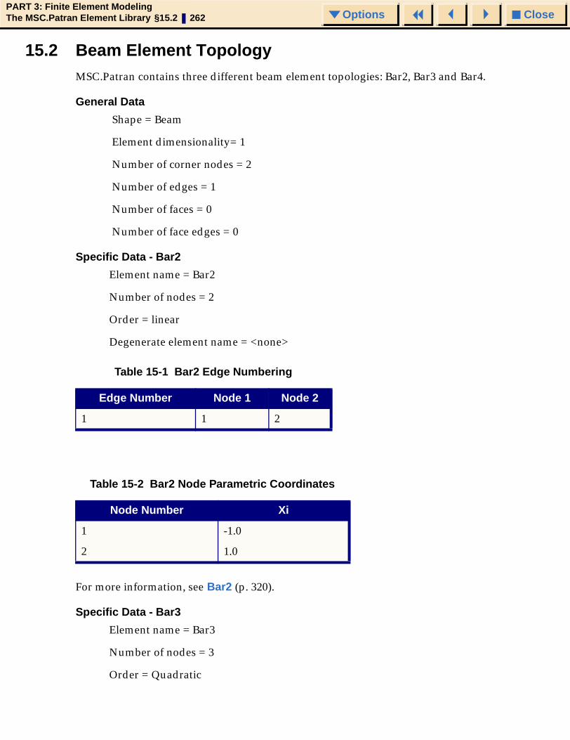
CloseOptionsPART 3: Finite Element ModelingThe MSC.Patran Element Library §15.2 262 Options
15.2 Beam Element TopologyMSC.Patran contains three different beam element topologies: Bar2, Bar3 and Bar4.
General Data
Shape = Beam
Element dimensionality= 1
Number of corner nodes = 2
Number of edges = 1
Number of faces = 0
Number of face edges = 0
Specific Data - Bar2
Element name = Bar2
Number of nodes = 2
Order = linear
Degenerate element name = <none>
For more information, see Bar2 (p. 320).
Specific Data - Bar3
Element name = Bar3
Number of nodes = 3
Order = Quadratic
Table 15-1 Bar2 Edge Numbering
Edge Number Node 1 Node 2
1 1 2
Table 15-2 Bar2 Node Parametric Coordinates
Node Number Xi
1 -1.0
2 1.0

CloseOptionsPART 3: Finite Element ModelingThe MSC.Patran Element Library §15.2 263 Options
Degenerate element name = <none>
For more information, see Bar3 (p. 322).
Specific Data - Bar4
Element name = Bar4
Number of nodes = 4
Order = Cubic
Degenerate element name = <none>
For more information, see Bar4 (p. 330).
Table 15-3 Bar3 Edge Numbering
Edge Number Node 1 Node 2 Node 3
1 1 3 2
Table 15-4 Bar3 Node Parametric Coordinates
Node Number Xi
1 -1.0
2 1.0
3 0.0
Table 15-5 Bar4 Edge Numbering
Edge Number Node 1 Node 2 Node 3 Node 4
1 1 3 4 2
Table 15-6 Bar4 Node Parametric Coordinates
Node Number Xi
1 -1.0
2 1.0
3 -1/3
4 1/3

CloseOptionsPART 3: Finite Element ModelingThe MSC.Patran Element Library §15.3 264 Options
15.3 Tria Element TopologyMSC.Patran contains six different triangular element topologies: Tria3, Tria4, Tria6, Tria7, Tria9, Tria13.
General Shape
For Tri elements, area coordinates [L1/L2/L3] are commonly used. See Area (p. 260) coordinate system for more information.
Tri elements can be obtained by degenerating a Quad element.
1. Quad corner node 2 collapses onto 1.
2. Tri corner nodes 1/2/3 match 1/3/4 for the Quad.
General Data
Shape = Triangular
Element dimensionality= 2
Number of corner nodes = 3
Number of edges = 3
Number of faces = 1
Number of face edges = 3
Specific Data - Tria3
Element name = Tria3
Number of nodes = 3
Order = linear
Degenerate element name = <none>
Table 15-7 Tria Face Numbering
Face ID Sense Edge 1 Edge 2 Edge 3
1 1 1 2 3
Table 15-8 Tria3 Edge Numbering
Edge Number Node 1 Node 2
1 1 2
2 2 3
3 3 1

CloseOptionsPART 3: Finite Element ModelingThe MSC.Patran Element Library §15.3 265 Options
To obtain a Tri3 by degenerating a Quad4, the following are corresponding nodes:
For more information, see Tri3 (p. 320).
Specific Data - Tria4
Element name = Tria4
Number of nodes = 4
Order = linear
Degenerate element name = <none>
Table 15-9 Tria3 Node Parametric Coordinates
Node Number Xi/Eta or L2/L3
1 0.0, 0.0
2 1.0, 0.0,0.0
3 0.0, 1.0
Tri3 Quad4
1 1
2 3
3 4
Table 15-10 Tria4 Edge Numbering
Edge Number Node 1 Node 2
1 1 2
2 2 3
3 3 1
Table 15-11 Tria4 Node Parametric Coordinates
Node Number Xi/Eta or L2/L3
1 0.0, 0.0
2 1.0, 0.0

CloseOptionsPART 3: Finite Element ModelingThe MSC.Patran Element Library §15.3 266 Options
To obtain a Tri4 by degenerating a Quad5, the following are corresponding nodes:
For more information, see Tri4 (p. 321).
Specific Data - Tria6
Element name = Tria6
Number of nodes = 6
Order = Quadratic
Degenerate element name = <none>
3 0.0, 1.0
4 1/3, 1/3
Tri4 Quad5
1 1
2 3
3 4
4 5
Table 15-12 Tria6 Edge Numbering
Edge Number Node 1 Node 2 Node 3
1 1 4 2
2 2 5 3
3 3 6 1
Table 15-13 Tria6 Node Parametric Coordinates
Node Number Xi/Eta or L2/L3
1 0.0, 0.0
2 1.0, 0.0
3 0.0, 1.0
4 0.5, 0.0
Table 15-11 Tria4 Node Parametric Coordinates
Node Number Xi/Eta or L2/L3

CloseOptionsPART 3: Finite Element ModelingThe MSC.Patran Element Library §15.3 267 Options
To obtain a Tri6 by degenerating a Quad8, the following are corresponding nodes:
For more information, see Tri6 (p. 322).
Specific Data - Tria7
Element name = Tria7
Number of nodes = 7
Order = Quadratic
Degenerate element name = <none>
5 0.5, 0.5
6 0.0, 0.5
Tri6 Quad8
1 1
2 3
3 4
4 6
5 7
6 8
Table 15-14 Tria7 Edge Numbering
Edge Number Node 1 Node 2 Node 3
1 1 4 2
2 2 5 3
3 3 6 1
Table 15-15 Tria7 Node Parametric Coordinates
Node Number Xi/Eta or L2/L3
1 0.0, 0.0
2 1.0, 0.0
3 0.0, 1.0
4 0.5, 0.0
Table 15-13 Tria6 Node Parametric Coordinates
Node Number Xi/Eta or L2/L3

CloseOptionsPART 3: Finite Element ModelingThe MSC.Patran Element Library §15.3 268 Options
To obtain a Tri7 by degenerating a Quad9, the following are corresponding nodes:
For more information, see Tri7 (p. 323).
Specific Data - Tria9
Element name = Tria9
Number of nodes = 9
Order = Cubic
Degenerate element name = <none>
5 0.5, 0.5
6 0.0, 0.5
7 1/3, 1/3
Tri7 Quad9
1 1
2 3
3 4
4 6
5 7
6 8
7 9
Table 15-16 Tria9 Edge Numbering
Edge Number Node 1 Node 2 Node 3 Node 4
1 1 4 5 2
2 2 6 7 3
3 3 8 9 1
Table 15-17 Tria9 Node Parametric Coordinates
Node Number Xi/Eta or L2/L3
1 0.0, 0.0
2 1.0, 0.0
3 0.0, 1.0
Table 15-15 Tria7 Node Parametric Coordinates
Node Number Xi/Eta or L2/L3

CloseOptionsPART 3: Finite Element ModelingThe MSC.Patran Element Library §15.3 269 Options
To obtain a Tri9 by degenerating a Quad12, the following are corresponding nodes:
For more information, see Tri9 (p. 330).
Specific Data - Tria13
Element name = Tria13
Number of nodes = 13
Order = Cubic
Degenerate element name = <none>
4 1/3, 0.0
5 2/3, 0.0
6 1/3, 2/3
7 1/3, 2/3
8 0.0, 2/3
9 0.0, 1/3
Tri9 Quad12
1 1
2 3
3 4
4 7
5 8
6 9
7 10
8 11
9 12
Table 15-18 Tria13 Edge Numbering
Edge Number Node 1 Node 2 Node 3 Node 4
1 1 4 5 2
2 2 6 7 3
3 3 8 9 1
Table 15-17 Tria9 Node Parametric Coordinates
Node Number Xi/Eta or L2/L3

CloseOptionsPART 3: Finite Element ModelingThe MSC.Patran Element Library §15.3 270 Options
To obtain a Tri13 by degenerating a Quad16, the following are corresponding nodes:
For more information, see Tri13 (p. 331).
Table 15-19 Tria13 Node Parametric Coordinates
Node Number Xi/Eta or L2/L3
1 0.0, 0.0
2 1.0, 0.0
3 0.0, 1.0
4 1/3, 0.0
5 2/3, 0.0
6 2/3, 1/3
7 1/3, 2/3
8 0.0, 2/3
9 0.0, 1/3
10 2/9, 1/9
11 4/9, 2/9
12 2/9, 4/9
13 1/9, 2/9
Tri13 Quad16
1 1
2 3
3 4
4 7
5 8
6 9
7 10
8 11
9 12
10 14
11 15
12 16
13 13

CloseOptionsPART 3: Finite Element ModelingThe MSC.Patran Element Library §15.4 271 Options
15.4 Quad Element TopologyMSC.Patran contains six different quadrilateral element topologies: Quad4, Quad5, Quad8, Quad9, Quad12, Quad16.
General Data
Shape = Quadrilateral
Element dimensionality= 2
Number of corner nodes = 4
Number of edges = 4
Number of faces = 1
Number of face edges = 4
Specific Data - Quad4
Element name = Quad4
Number of nodes = 4
Order = linear
Degenerate element name = Tria3
Table 15-20 Quad Face Numbering
Face ID Sense Edge 1 Edge 2 Edge 3 Edge 4
1 1 1 2 3 4
Table 15-21 Quad4 Edge Numbering
Edge Number Node 1 Node 2
1 1 2
2 2 3
3 3 4
4 4 1

CloseOptionsPART 3: Finite Element ModelingThe MSC.Patran Element Library §15.4 272 Options
For more information, see Quad4 (p. 320).
Specific Data - Quad5
Element name = Quad5
Number of nodes = 5
Order = linear
Degenerate element name = Tria4
Table 15-22 Quad4 Node Parametric Coordinates
Node Number Xi/Eta
1 -1.0, -1.0
2 1.0, -1.0
3 1.0, 1.0
4 -1.0, 1.0
Table 15-23 Quad5 Edge Numbering
Edge Number Node 1 Node 2
1 1 2
2 2 3
3 3 4
4 4 1
Table 15-24 Quad5 Node Parametric Coordinates
Node Number Xi/Eta
1 -1.0, -1.0
2 1.0, -1.0
3 1.0, 1.0
4 -1.0, 1.0
5 0.0, 0.0

CloseOptionsPART 3: Finite Element ModelingThe MSC.Patran Element Library §15.4 273 Options
For more information, see Quad5 (p. 321).
Specific Data - Quad8
Element name = Quad8
Number of nodes = 8
Order = Quadratic
Degenerate element name = Tria6
For more information, see Quad8 (p. 322).
Specific Data - Quad9
Element name = Quad9
Number of nodes = 9
Order = Quadratic
Table 15-25 Quad8 Edge Numbering
Edge Number Node 1 Node 2 Node 3
1 1 5 2
2 2 6 3
3 3 7 4
4 4 8 1
Table 15-26 Quad8 Node Parametric Coordinates
Node Number Xi/Eta
1 -1.0, -1.0
2 1.0, -1.0
3 1.0, 1.0
4 -1.0, 1.0
5 0.0, -1.0
6 1.0, 0.0
7 0.0, 1.0
8 -1.0, 0.0
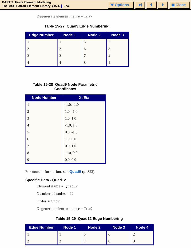
CloseOptionsPART 3: Finite Element ModelingThe MSC.Patran Element Library §15.4 274 Options
Degenerate element name = Tria7
For more information, see Quad9 (p. 323).
Specific Data - Quad12
Element name = Quad12
Number of nodes = 12
Order = Cubic
Degenerate element name = Tria9
Table 15-27 Quad9 Edge Numbering
Edge Number Node 1 Node 2 Node 3
1 1 5 2
2 2 6 3
3 3 7 4
4 4 8 1
Table 15-28 Quad9 Node ParametricCoordinates
Node Number Xi/Eta
1 -1.0, -1.0
2 1.0, -1.0
3 1.0, 1.0
4 -1.0, 1.0
5 0.0, -1.0
6 1.0, 0.0
7 0.0, 1.0
8 -1.0, 0.0
9 0.0, 0.0
Table 15-29 Quad12 Edge Numbering
Edge Number Node 1 Node 2 Node 3 Node 4
1 1 5 6 2
2 2 7 8 3

CloseOptionsPART 3: Finite Element ModelingThe MSC.Patran Element Library §15.4 275 Options
For more information, see Quad12 (p. 330).
Specific Data - Quad16
Element name = Quad16
Number of nodes = 16
Order = Cubic
Degenerate element name = Tria13
3 3 9 10 4
4 4 11 12 1
Table 15-30 Quad12 Node Parametric Coordinates
Node Number Xi/Eta
1 -1.0, -1.0
2 1.0, -1.0
3 1.0, 1.0
4 -1.0, 1.0
5 1/3, -1.0
6 1/3, -1.0
7 1.0,-1/3
8 1.0,1/3
9 1/3, 1.0
10 -1/3, 1.0
11 -1.0,1/3
12 -1.0,-1/3
Table 15-31 Quad16 Edge Numbering
Edge Number Node 1 Node 2 Node 3 Node 4
1 1 5 6 2
2 2 7 8 3
Table 15-29 Quad12 Edge Numbering
Edge Number Node 1 Node 2 Node 3 Node 4

CloseOptionsPART 3: Finite Element ModelingThe MSC.Patran Element Library §15.4 276 Options
For more information, see Quad16 (p. 331).
3 3 9 10 4
4 4 11 12 1
Table 15-32 Quad16 Node Parametric Coordinates
Node Number Xi/Eta
1 -1.0, -1.0
2 1.0, -1.0
3 1.0, 1.0
4 -1.0, 1.0
5 -1/3, -1.0
6 1/3, -1.0
7 1.0,-1/3
8 1.0,1/3
9 1/3, 1.0
10 -1/3, 1.0
11 -1.0,1/3
12 -1.0,-1/3
13 -1/3,-1/3
14 1/3, -1/3
15 1/3, 1/3
16 -1/3, 1/3
Table 15-31 Quad16 Edge Numbering
Edge Number Node 1 Node 2 Node 3 Node 4
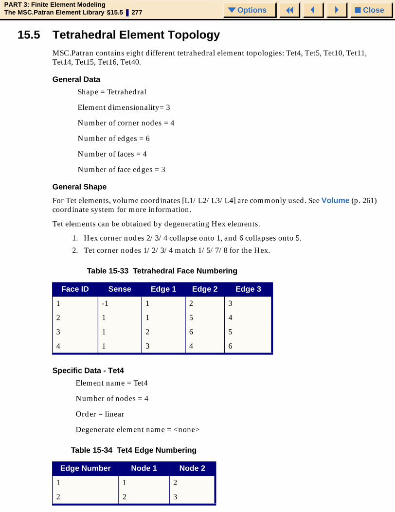
CloseOptionsPART 3: Finite Element ModelingThe MSC.Patran Element Library §15.5 277 Options
15.5 Tetrahedral Element TopologyMSC.Patran contains eight different tetrahedral element topologies: Tet4, Tet5, Tet10, Tet11, Tet14, Tet15, Tet16, Tet40.
General Data
Shape = Tetrahedral
Element dimensionality= 3
Number of corner nodes = 4
Number of edges = 6
Number of faces = 4
Number of face edges = 3
General Shape
For Tet elements, volume coordinates [L1/L2/L3/L4] are commonly used. See Volume (p. 261) coordinate system for more information.
Tet elements can be obtained by degenerating Hex elements.
1. Hex corner nodes 2/3/4 collapse onto 1, and 6 collapses onto 5.
2. Tet corner nodes 1/2/3/4 match 1/5/7/8 for the Hex.
Specific Data - Tet4
Element name = Tet4
Number of nodes = 4
Order = linear
Degenerate element name = <none>
Table 15-33 Tetrahedral Face Numbering
Face ID Sense Edge 1 Edge 2 Edge 3
1 -1 1 2 3
2 1 1 5 4
3 1 2 6 5
4 1 3 4 6
Table 15-34 Tet4 Edge Numbering
Edge Number Node 1 Node 2
1 1 2
2 2 3

CloseOptionsPART 3: Finite Element ModelingThe MSC.Patran Element Library §15.5 278 Options
To obtain a Tet4 by degenerating a Hex8, the following are corresponding nodes:
For more information, see Tet4 (p. 320).
Specific Data - Tet5
Element name = Tet5
Number of nodes = 5
Order = linear
Degenerate element name = <none>
3 3 1
4 1 4
5 2 4
6 3 4
Table 15-35 Tet4 Node Parametric Coordinates
Node Number Xi/Eta/Zeta or L2/L3/L4
1 0.0, 0.0, 0.0
2 1.0, 0.0, 0.0
3 0.0, 1.0, 0.0
4 0.0, 0.0, 1.0
Tet4 Hex8
1 1
2 5
3 7
4 8
Table 15-36 Tet5 Edge Numbering
Edge Number Node 1 Node 2
1 1 2
2 2 3
Table 15-34 Tet4 Edge Numbering
Edge Number Node 1 Node 2

CloseOptionsPART 3: Finite Element ModelingThe MSC.Patran Element Library §15.5 279 Options
To obtain a Tet5 by degenerating a Hex9, the following are corresponding nodes:
For more information, see Tet5 (p. 321).
Specific Data - Tet10
Element name = Tet10
Number of nodes = 10
Order = Quadratic
3 3 1
4 1 4
5 2 4
6 3 4
Table 15-37 Tet5 Node Parametric Coordinates
Node Number Xi/Eta/Zeta or L2/L3/L4
1 0.0, 0.0, 0.0
2 1.0, 0.0, 0.0
3 0.0, 1.0, 1.0
4 0.0, 0.0, 1.0
5 1/4, 1/4, 1/4
Tet5 Hex9
1 1
2 5
3 7
4 8
5 9
Table 15-36 Tet5 Edge Numbering
Edge Number Node 1 Node 2

CloseOptionsPART 3: Finite Element ModelingThe MSC.Patran Element Library §15.5 280 Options
Degenerate element name = <none>
To obtain a Tet10 by degenerating a Hex20, the following are corresponding nodes:
Table 15-38 Tet10 Edge Numbering
Edge Number Node 1 Node 2 Node 3
1 1 5 2
2 2 6 3
3 3 7 1
4 1 8 4
5 2 9 4
6 3 10 4
Table 15-39 Tet10 Node Parametric Coordinates
Node Number Xi/Eta/Zeta or L2/L3/L4
1 0.0, 0.0, 0.0
2 1.0, 0.0, 0.0
3 0.0, 1.0, 0.0
4 0.0, 0.0, 1.0
5 0.5, 0.0, 0.0
6 0.5, 0.5, 0.0
7 0.0, 0.5, 0.0
8 0.0, 0.0, 0.5
9 0.5, 0.0, 0.5
10 0.0, 0.5, 0.5
Tet10 Hex20
1 1
2 5
3 7
4 8
5 13
6 18
7 15
8 16

CloseOptionsPART 3: Finite Element ModelingThe MSC.Patran Element Library §15.5 281 Options
For more information, see Tet10 (p. 322).
Specific Data - Tet11
Element name = Tet11
Number of nodes = 11
Order = Quadratic
Degenerate element name = <none>
9 20
10 19
Table 15-40 Tet11 Edge Numbering
Edge Number Node 1 Node 2 Node 3
1 1 5 2
2 2 6 3
3 3 7 1
4 1 8 4
5 2 9 4
6 3 10 4
Table 15-41 Tet11 Node Parametric Coordinates
Node Number Xi/Eta/Zeta or L2/L3/L4
1 0.0, 0.0, 0.0
2 1.0, 0.0, 0.0
3 0.0, 1.0, 0.0
4 0.0, 0.0, 1.0
5 0.5, 0.0, 0.0
6 0.5, 0.5, 0.0
7 0.0, 0.5, 0.0
8 0.0, 0.0, 0.5
9 0.5, 0.0, 0.5
10 0.0, 0.5, 0.5
11 1/4, 1/4, 1/4
Tet10 Hex20

CloseOptionsPART 3: Finite Element ModelingThe MSC.Patran Element Library §15.5 282 Options
To obtain a Tet11 by degenerating a Hex21, the following are corresponding nodes:
For more information, see Tet11 (p. 323).
Specific Data - Tet14
Element name = Tet14
Number of nodes = 14
Order = Quadratic
Degenerate element name = <none>
Tet11 Hex21
1 1
2 5
3 7
4 8
5 13
6 18
7 15
8 16
9 20
10 19
11 21
Table 15-42 Tet14 Edge Numbering
Edge Number Node 1 Node 2 Node 3
1 1 5 2
2 2 6 3
3 3 7 1
4 1 8 4
5 2 9 4
6 3 10 4

CloseOptionsPART 3: Finite Element ModelingThe MSC.Patran Element Library §15.5 283 Options
To obtain a Tet14 by degenerating a Hex27, the following are corresponding nodes:
Table 15-43 Tet14 Node Parametric Coordinates
Node Number Xi/Eta/Zeta or L2/L3/L4
1 0.0, 0.0, 0.0
2 1.0, 0.0, 0.0
3 0.0, 1.0, 0.0
4 0.0, 0.0, 1.0
5 0.5, 0.0, 0.0
6 0.5, 0.5, 0.0
7 0.0, 0.5, 0.0
8 0.0, 0.0, 0.5
9 0.5, 0.0, 0.5
10 0.0, 0.5, 0.5
11 1/4, 1/4, 0.0
12 0.5, 1/4, 1/4
13 0.0, 1/4, 1/4
14 1/4, 0.0, 1/4
Tet14 Hex27
1 1
2 5
3 7
4 8
5 13
6 18
7 15
8 16
9 20
10 19
11 25
12 23
13 27
14 24

CloseOptionsPART 3: Finite Element ModelingThe MSC.Patran Element Library §15.5 284 Options
For more information, see Tet14 (p. 324).
Specific Data - Tet15
Element name = Tet15
Number of nodes = 15
Order = Quadratic
Degenerate element name = <none>
Table 15-44 Tet15 Edge Numbering
Edge Number Node 1 Node 2 Node 3
1 1 5 2
2 2 6 3
3 3 7 1
4 1 8 4
5 2 9 4
6 3 10 4
Table 15-45 Tet15 Node Parametric Coordinates
Node Number Xi/Eta/Zeta or L2/L3/L4
1 0.0, 0.0, 0.0
2 1.0, 0.0, 0.0
3 0.0, 1.0, 0.0
4 0.0, 0.0, 1.0
5 0.5, 0.0, 0.0
6 0.5, 0.5, 0.0
7 0.0, 0.5, 0.0
8 0.0, 0.0, 0.5
9 0.5, 0.0, 0.5
10 0.0, 0.5, 0.5
11 1/4, 1/4, 1/4
12 1/4, 1/4, 0.0
13 0.5, 1/4, 1/4
14 0.0, 1/4, 1/4
15 1/4, 0.0, 1/4
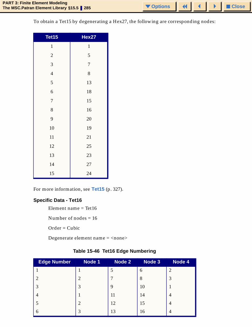
CloseOptionsPART 3: Finite Element ModelingThe MSC.Patran Element Library §15.5 285 Options
To obtain a Tet15 by degenerating a Hex27, the following are corresponding nodes:
For more information, see Tet15 (p. 327).
Specific Data - Tet16
Element name = Tet16
Number of nodes = 16
Order = Cubic
Degenerate element name = <none>
Tet15 Hex27
1 1
2 5
3 7
4 8
5 13
6 18
7 15
8 16
9 20
10 19
11 21
12 25
13 23
14 27
15 24
Table 15-46 Tet16 Edge Numbering
Edge Number Node 1 Node 2 Node 3 Node 4
1 1 5 6 2
2 2 7 8 3
3 3 9 10 1
4 1 11 14 4
5 2 12 15 4
6 3 13 16 4

CloseOptionsPART 3: Finite Element ModelingThe MSC.Patran Element Library §15.5 286 Options
To obtain a Tet16 by degenerating a Hex32, the following are corresponding nodes:
Table 15-47 Tet16 Node Parametric Coordinates
Node Number Xi/Eta/Zeta or L2/L3/L4
1 0.0, 0.0, 0.0
2 1.0, 0.0, 0.0
3 0.0, 1.0, 0.0
4 0.0, 0.0, 1.0
5 1/3, 0.0, 0.0
6 2/3, 0.0, 0.0
7 2/3,1/3, 0.0
8 1/3, 2/3, 0.0
9 0.0, 2/3, 0.0
10 0.0, 1/3, 0.0
11 0.0, 0.0, 1/3
12 2/3, 0.0, 1/3
13 0.0, 1/3, 2/3
14 0.0, 0.0, 2/3
15 1/3, 0.0, 2/3
16 0.0, 1/3, 2/3
Tet16 Hex32
1 1
2 5
3 7
4 8
5 17
6 21
7 27
8 28
9 23
10 19
11 20
12 32

CloseOptionsPART 3: Finite Element ModelingThe MSC.Patran Element Library §15.5 287 Options
For more information, see Tet16 (p. 330).
Specific Data - Tet40
Element name = Tet40
Number of nodes = 40
Order = Cubic
Degenerate element name = <none>
13 29
14 24
15 31
16 30
Table 15-48 Tet40 Edge Numbering
Edge Number Node 1 Node 2 Node 3 Node 4
1 1 5 6 2
2 2 7 8 3
3 3 9 10 1
4 1 11 14 4
5 2 12 15 4
6 3 13 16 4
Table 15-49 Tet40 Node Parametric Coordinates
Node Number C(3) Node Number Xi/Eta/Zeta or L2/L3/L4
1 0.0, 0.0, 0.0 21 2/9, 0.0, 1/9
2 1.0, 0.0, 0.0 22 4/9, 0.0, 2/9
3 0.0, 1.0, 0.0 23 2/3, 2/9, 1/9
4 0.0, 0.0, 1.0 24 1/3, 4/9, 2/9
5 1/3, 0.0, 0.0 25 0.0, 1/9, 2/9
6 2/3, 0.0, 0.0 26 0.0, 2/9, 1/9
7 2/3, 1/3, 0.0 27 2/9,.074074,.037037
8 1/3, 2/3, 0.0 28 4/9, 148148,.074074
9 0.0, 2/3, 0.0 29 2/9, .296297,.148148
Tet16 Hex32

CloseOptionsPART 3: Finite Element ModelingThe MSC.Patran Element Library §15.5 288 Options
To obtain a Tet40 by degenerating a Hex64, the following are corresponding nodes:
10 0.0, 1/3,0.0 30 1/9,.148148, .074074
11 0.0, 0.0, 1/3 31 1/9, 0.0, 2/9
12 2/3, 0.0, 1/3 32 2/9, 0.0, 4/9
13 0.0, 2/3, 1/3 33 2/3, 1/9, 2/9
14 0.0, 0.0, 2/3 34 1/3, 2/9, 4/9
15 1/3, 0.0, 2/3 35 0.0, 2/9, 4/9
16 0.0, 1/3, 2/3 36 0.0, 4/9, 2/9
17 2/9, 1/9, 0.0 37 2/9,.037037,.074074
18 4/9, 2/9, 0.0 38 4/9,.074074,.148148
19 2/9, 4/9, 0.0 39 2/9,.148148,.296297
20 1/9, 2/9, 0.0 40 1/9,.074074,.148148
Tet40 Hex64
1 1
2 5
3 7
4 8
5 17
6 21
7 27
8 28
9 23
10 19
11 20
12 32
13 29
14 24
15 31
16 30
17 39
Table 15-49 Tet40 Node Parametric Coordinates
Node Number C(3) Node Number Xi/Eta/Zeta or L2/L3/L4

CloseOptionsPART 3: Finite Element ModelingThe MSC.Patran Element Library §15.5 289 Options
For more information, see Tet40 (p. 332).
18 51
19 52
20 40
21 44
22 56
23 62
24 63
25 42
26 41
27 46
28 58
29 59
30 47
31 43
32 55
33 61
34 64
35 54
36 53
37 45
38 57
39 60
40 48
Tet40 Hex64

CloseOptionsPART 3: Finite Element ModelingThe MSC.Patran Element Library §15.6 290 Options
15.6 Wedge Element TopologyMSC.Patran contains eight different wedge element topologies: Wedge6, Wedge7, Wedge15, Wedge16, Wedge20, Wedge21, Wedge24 and Wedge52.
General Data
Shape = Wedge
Element dimensionality= 3
Number of corner nodes = 6
Number of edges = 9
Number of faces = 5
Number of face edges = 4,3
General Shape
For Wedge elements, a combination of area and rectangular coordinates [L1/L2/L3/Zeta] are commonly used. Zeta values vary from -1 to 1 as in a Hex element. The area coordinates L1/L2/L3 represent the weighting with respect to the 3 edges along the Zeta direction:
edge number 8 (node 1-->4)
edge number 7 (node 2-->5)
edge number 9 (node 3-->6)
See Area (p. 260) coordinate system for more information.
Wedge elements can be obtained by degenerating Hex elements.
1. Hex corner node 2 collapses onto 1, and 6 collapses onto 5.
2. Wedge corner nodes 1:6 match 1/3/4/5/7/8 for the Hex.
Specific Data - Wedge6
Element name = Wedge6
Number of nodes = 6
Order = linear
Table 15-50 Wedge Face Numbering
Face ID Sense Edge 1 Edge 2 Edge 3 Edge 4
1 1 1 2 3 *
2 -1 4 5 6 *
3 -1 1 8 4 7
4 -1 2 9 5 8
5 -1 3 7 6 9

CloseOptionsPART 3: Finite Element ModelingThe MSC.Patran Element Library §15.6 291 Options
Degenerate element name = Tet4
To obtain a Wedge6 by degenerating a Hex8, the following are corresponding nodes:
Table 15-51 Wedge6 Edge Numbering
Edge Number Node 1 Node 2
1 2 1
2 1 3
3 3 2
4 5 4
5 4 6
6 6 5
7 2 5
8 1 4
9 3 6
Table 15-52 Wedge6 Node Parametric Coordinates
Node Number Xi/Eta/Zeta or L2/L3/Zeta
1 0.0, 0.0, -1.0
2 1.0, 0.0, -1.0
3 0.0, 1.0, -1.0
4 0.0, 0.0, 1.0
5 1.0, 0.0, 1.0
6 0.0, 1.0, 1.0
Wedge6 Hex8
1 1
2 3
3 4
4 5
5 7
6 8

CloseOptionsPART 3: Finite Element ModelingThe MSC.Patran Element Library §15.6 292 Options
For more information, see Wedge 6 (p. 320).
Specific Data - Wedge7
Element name = Wedge7
Number of nodes = 7
Order = linear
Degenerate element name = Tet5
Table 15-53 Wedge7 Edge Numbering
Edge Number Node 1 Node 2
1 2 1
2 1 3
3 3 2
4 5 4
5 4 6
6 6 5
7 2 5
8 1 4
9 3 6
Table 15-54 Wedge7 Node Parametric Coordinates
Node Number Xi/Eta/Zeta or L2/L3/Zeta
1 0.0, 0.0, -1.0
2 1.0, 0.0, -1.0
3 0.0, 1.0, -1.0
4 0.0, 0.0, 1.0
5 1.0, 0.0, 1.0
6 0.0, 1.0, 1.0
7 1/3, 1/3, 0.0
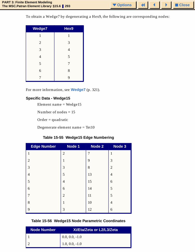
CloseOptionsPART 3: Finite Element ModelingThe MSC.Patran Element Library §15.6 293 Options
To obtain a Wedge7 by degenerating a Hex9, the following are corresponding nodes:
For more information, see Wedge7 (p. 321).
Specific Data - Wedge15
Element name = Wedge15
Number of nodes = 15
Order = quadratic
Degenerate element name = Tet10
Wedge7 Hex9
1 1
2 3
3 4
4 5
5 7
6 8
7 9
Table 15-55 Wedge15 Edge Numbering
Edge Number Node 1 Node 2 Node 3
1 2 7 1
2 1 9 3
3 3 8 2
4 5 13 4
5 4 15 6
6 6 14 5
7 2 11 5
8 1 10 4
9 3 12 6
Table 15-56 Wedge15 Node Parametric Coordinates
Node Number Xi/Eta/Zeta or L2/L3/Zeta
1 0.0, 0.0, -1.0
2 1.0, 0.0, -1.0
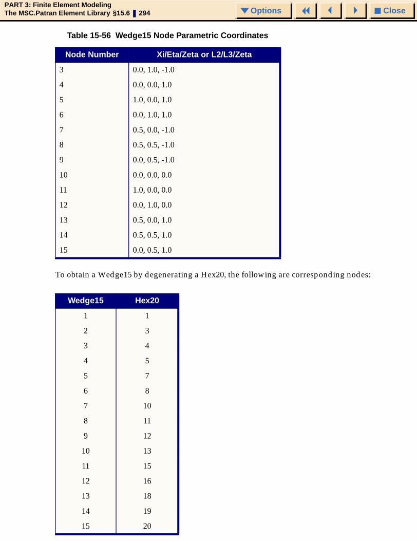
CloseOptionsPART 3: Finite Element ModelingThe MSC.Patran Element Library §15.6 294 Options
To obtain a Wedge15 by degenerating a Hex20, the following are corresponding nodes:
3 0.0, 1.0, -1.0
4 0.0, 0.0, 1.0
5 1.0, 0.0, 1.0
6 0.0, 1.0, 1.0
7 0.5, 0.0, -1.0
8 0.5, 0.5, -1.0
9 0.0, 0.5, -1.0
10 0.0, 0.0, 0.0
11 1.0, 0.0, 0.0
12 0.0, 1.0, 0.0
13 0.5, 0.0, 1.0
14 0.5, 0.5, 1.0
15 0.0, 0.5, 1.0
Wedge15 Hex20
1 1
2 3
3 4
4 5
5 7
6 8
7 10
8 11
9 12
10 13
11 15
12 16
13 18
14 19
15 20
Table 15-56 Wedge15 Node Parametric Coordinates
Node Number Xi/Eta/Zeta or L2/L3/Zeta

CloseOptionsPART 3: Finite Element ModelingThe MSC.Patran Element Library §15.6 295 Options
For more information, see Wedge15 (p. 322).
Specific Data - Wedge16
Element name = Wedge16
Number of nodes = 16
Order = quadratic
Degenerate element name = Tet11
Table 15-57 Wedge16 Edge Numbering
Edge Number Node 1 Node 2 Node 3
1 2 7 1
2 1 9 3
3 3 8 2
4 5 13 4
5 4 15 6
6 6 14 5
7 2 11 5
8 1 10 4
9 3 12 6
Table 15-58 Wedge16 Node Parametric Coordinates
Node Number Xi/Eta/Zeta or L2/L3/Zeta
1 0.0, 0.0, -1.0
2 1.0, 0.0, -1.0
3 0.0, 1.0, -1.0
4 0.0, 0.0, 1.0
5 1.0, 0.0, 1.0
6 0.0, 1.0, 1.0
7 0.5, 0.0, -1.0
8 0.5, 0.5, -1.0
9 0.0, 0.5, -1.0
10 0.0, 0.0, 0.0
11 1.0, 0.0, 0.0

CloseOptionsPART 3: Finite Element ModelingThe MSC.Patran Element Library §15.6 296 Options
To obtain a Wedge16 by degenerating a Hex21, the following are corresponding nodes:
For more information, see Wedge16 (p. 323).
Specific Data - Wedge20
Element name = Wedge20
Number of nodes = 20
Order = quadratic
12 0.0, 1.0, 0.0
13 0.5, 0.0, 1.0
14 0.5, 0.5, 1.0
15 0.0, 0.5, 1.0
16 1/3, 1/3, 0.0
Wedge16 Hex21
1 1
2 3
3 4
4 5
5 7
6 8
7 10
8 11
9 12
10 13
11 15
12 16
13 18
14 19
15 20
16 21
Table 15-58 Wedge16 Node Parametric Coordinates
Node Number Xi/Eta/Zeta or L2/L3/Zeta

CloseOptionsPART 3: Finite Element ModelingThe MSC.Patran Element Library §15.6 297 Options
Degenerate element name = Tet14
Table 15-59 Wedge20 Edge Numbering
Edge Number Node 1 Node 2 Node 3
1 2 7 1
2 1 9 3
3 3 8 2
4 5 13 4
5 4 15 6
6 6 14 5
7 2 11 5
8 1 10 4
9 3 12 6
Table 15-60 Wedge20 Node Parametric Coordinates
Node Number Xi/Eta/Zeta or L2/L3/Zeta
1 0.0, 0.0, -1.0
2 1.0, 0.0, -1.0
3 0.0, 1.0, -1.0
4 0.0, 0.0, 1.0
5 1.0, 0.0, 1.0
6 0.0, 1.0, 1.0
7 0.5, 0.0, -1.0
8 0.5, 0.5, -1.0
9 0.0, 0.5, -1.0
10 0.0, 0.0, 0.0
11 1.0, 0.0, 0.0
12 0.0, 1.0, 0.0
13 0.5, 0.0, 1.0
14 0.5, 0.5, 1.0
15 0.0, 0.5, 1.0
16 1/3, 1/3, -1.0

CloseOptionsPART 3: Finite Element ModelingThe MSC.Patran Element Library §15.6 298 Options
To obtain a Wedge20 by degenerating a Hex26, the following are corresponding nodes:
For more information, see Wedge20 (p. 325).
17 1/3, 1/3, 1.0
18 0.5, 0.5, 0.0
19 0.0, 0.5, 0.0
20 0.5, 0.0, 0.0
Wedge20 Hex26
1 1
2 3
3 4
4 5
5 7
6 8
7 10
8 11
9 12
10 13
11 15
12 16
13 18
14 19
15 20
16 21
17 22
18 26
19 23
20 24
Table 15-60 Wedge20 Node Parametric Coordinates
Node Number Xi/Eta/Zeta or L2/L3/Zeta

CloseOptionsPART 3: Finite Element ModelingThe MSC.Patran Element Library §15.6 299 Options
Specific Data - Wedge21
Element name = Wedge21
Number of nodes = 21
Order = quadratic
Degenerate element name = Tet15
Table 15-61 Wedge21 Edge Numbering
Edge Number Node 1 Node 2 Node 3
1 2 7 1
2 1 9 3
3 3 8 2
4 5 13 4
5 4 15 6
6 6 14 5
7 2 11 5
8 1 10 4
9 3 12 6
Table 15-62 Wedge21 Node Parametric Coordinates
Node Number Xi/Eta/Zeta or L2/L3/Zeta
1 0.0, 0.0, -1.0
2 1.0, 0.0, -1.0
3 0.0, 1.0, -1.0
4 0.0, 0.0, 1.0
5 1.0, 0.0, 1.0
6 0.0, 1.0, 1.0
7 0.5, 0.0, -1.0
8 0.5, 0.5, -1.0
9 0.0, 0.5, -1.0
10 0.0, 0.0, 0.0
11 1.0, 0.0, 0.0
12 0.0, 1.0, 0.0

CloseOptionsPART 3: Finite Element ModelingThe MSC.Patran Element Library §15.6 300 Options
To obtain a Wedge21 by degenerating a Hex27, the following are corresponding nodes:
13 0.5, 0.0, 1.0
14 0.5, 0.5, 1.0
15 0.0, 0.5, 1.0
16 1/3, 1/3, 0.0
17 1/3, 1/3, -1.0
18 1/3, 1/3, 1.0
19 0.5, 0.5, 0.0
20 0.0, 0.5, 0.0
21 0.5, 0.0, 0.0
Wedge21 Hex27
1 1
2 3
3 4
4 5
5 7
6 8
7 10
8 11
9 12
10 13
11 15
12 16
13 18
14 19
15 20
16 21
17 22
Table 15-62 Wedge21 Node Parametric Coordinates
Node Number Xi/Eta/Zeta or L2/L3/Zeta

CloseOptionsPART 3: Finite Element ModelingThe MSC.Patran Element Library §15.6 301 Options
For more information, see Wedge21 (p. 328).
Specific Data - Wedge24
Element name = Wedge24
Number of nodes = 24
Order = Cubic
Degenerate element name = Tet16
18 23
19 27
20 24
21 25
Table 15-63 Wedge24 Edge Numbering
Edge Number Node 1 Node 2 Node 3 Node 4
1 2 8 7 1
2 1 12 11 3
3 3 10 9 2
4 5 20 19 4
5 4 24 23 6
6 6 22 21 5
7 2 14 17 5
8 1 13 16 4
9 3 15 18 6
Table 15-64 Wedge24 Node Parametric Coordinates
Node Number Xi/Eta/Zeta or L2/L3/Zeta
1 0.0, 0.0, -1.0
2 1.0, 0.0, -1.0
3 0.0, 1.0, -1.0
4 0.0, 0.0, 1.0
5 1.0, 0.0, 1.0
Wedge21 Hex27
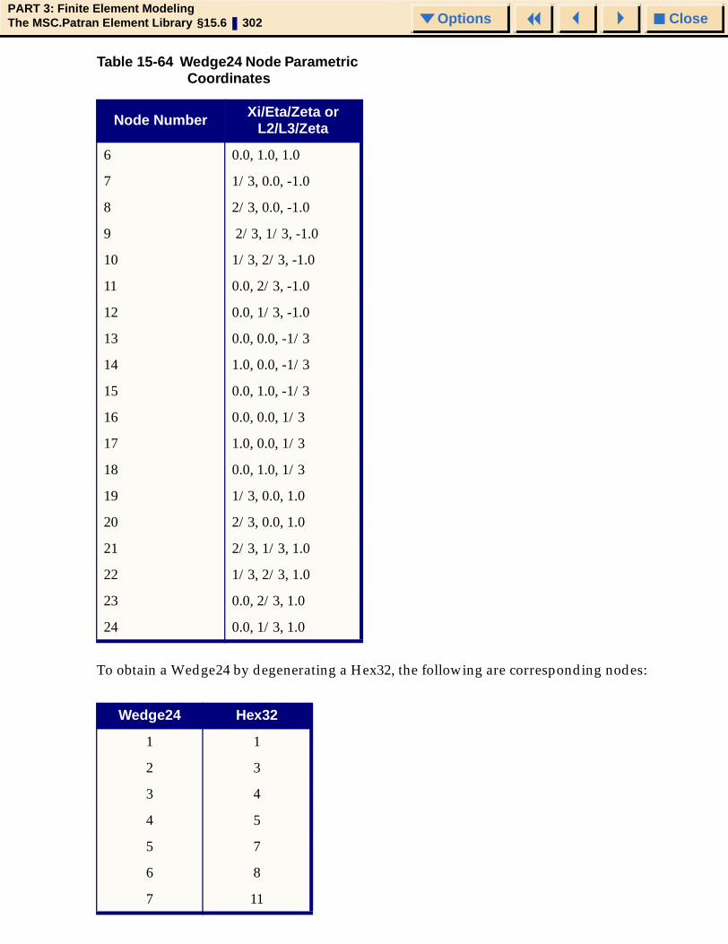
CloseOptionsPART 3: Finite Element ModelingThe MSC.Patran Element Library §15.6 302 Options
To obtain a Wedge24 by degenerating a Hex32, the following are corresponding nodes:
6 0.0, 1.0, 1.0
7 1/3, 0.0, -1.0
8 2/3, 0.0, -1.0
9 2/3, 1/3, -1.0
10 1/3, 2/3, -1.0
11 0.0, 2/3, -1.0
12 0.0, 1/3, -1.0
13 0.0, 0.0, -1/3
14 1.0, 0.0, -1/3
15 0.0, 1.0, -1/3
16 0.0, 0.0, 1/3
17 1.0, 0.0, 1/3
18 0.0, 1.0, 1/3
19 1/3, 0.0, 1.0
20 2/3, 0.0, 1.0
21 2/3, 1/3, 1.0
22 1/3, 2/3, 1.0
23 0.0, 2/3, 1.0
24 0.0, 1/3, 1.0
Wedge24 Hex32
1 1
2 3
3 4
4 5
5 7
6 8
7 11
Table 15-64 Wedge24 Node Parametric Coordinates
Node Number Xi/Eta/Zeta or L2/L3/Zeta

CloseOptionsPART 3: Finite Element ModelingThe MSC.Patran Element Library §15.6 303 Options
For more information, see Wedge24 (p. 330).
Specific Data - Wedge52
Element name = Wedge52
Number of nodes = 52
Order = Cubic
Degenerate element name = Tet40
8 12
9 13
10 14
11 15
12 16
13 17
14 19
15 20
16 21
17 23
18 24
19 27
20 28
21 29
22 30
23 31
24 32
Table 15-65 Wedge52 Edge Numbering
Edge Number Node 1 Node 2 Node 3 Node 4
1 2 8 7 1
2 1 12 11 3
3 3 10 9 2
4 5 20 19 4
5 4 24 23 6
Wedge24 Hex32
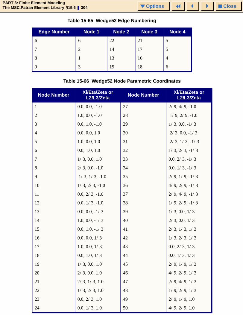
CloseOptionsPART 3: Finite Element ModelingThe MSC.Patran Element Library §15.6 304 Options
6 6 22 21 5
7 2 14 17 5
8 1 13 16 4
9 3 15 18 6
Table 15-66 Wedge52 Node Parametric Coordinates
Node Number Xi/Eta/Zeta or L2/L3/Zeta Node Number Xi/Eta/Zeta or
L2/L3/Zeta
1 0.0, 0.0, -1.0 27 2/9, 4/9, -1.0
2 1.0, 0.0, -1.0 28 1/9, 2/9, -1.0
3 0.0, 1.0, -1.0 29 1/3, 0.0, -1/3
4 0.0, 0.0, 1.0 30 2/3, 0.0, -1/3
5 1.0, 0.0, 1.0 31 2/3, 1/3, -1/3
6 0.0, 1.0, 1.0 32 1/3, 2/3, -1/3
7 1/3, 0.0, 1.0 33 0.0, 2/3, -1/3
8 2/3, 0.0, -1.0 34 0.0, 1/3, -1/3
9 1/3, 1/3, -1.0 35 2/9, 1/9, -1/3
10 1/3, 2/3, -1.0 36 4/9, 2/9, -1/3
11 0.0, 2/3, -1.0 37 2/9, 4/9, -1/3
12 0.0, 1/3, -1.0 38 1/9, 2/9, -1/3
13 0.0, 0.0, -1/3 39 1/3, 0.0, 1/3
14 1.0, 0.0, -1/3 40 2/3, 0.0, 1/3
15 0.0, 1.0, -1/3 41 2/3, 1/3, 1/3
16 0.0, 0.0, 1/3 42 1/3, 2/3, 1/3
17 1.0, 0.0, 1/3 43 0.0, 2/3, 1/3
18 0.0, 1.0, 1/3 44 0.0, 1/3, 1/3
19 1/3, 0.0, 1.0 45 2/9, 1/9, 1/3
20 2/3, 0.0, 1.0 46 4/9, 2/9, 1/3
21 2/3, 1/3, 1.0 47 2/9, 4/9, 1/3
22 1/3, 2/3, 1.0 48 1/9, 2/9, 1/3
23 0.0, 2/3, 1.0 49 2/9, 1/9, 1.0
24 0.0, 1/3, 1.0 50 4/9, 2/9, 1.0
Table 15-65 Wedge52 Edge Numbering
Edge Number Node 1 Node 2 Node 3 Node 4

CloseOptionsPART 3: Finite Element ModelingThe MSC.Patran Element Library §15.6 305 Options
To obtain a Wedge52 by degenerating a Hex64, the following are corresponding nodes:
25 2/9, 1/9, -1.0 51 2/9, 4/9, 1.0
26 4/9, 2/9, -1.0 52 1/9, 2/9, 1.0
Wedge52 Hex64
1 1
2 3
3 4
4 5
5 7
6 8
7 11
8 12
9 13
10 14
11 15
12 16
13 17
14 19
15 20
16 21
17 23
18 24
19 27
20 28
21 29
22 30
23 31
24 32
25 34
Table 15-66 Wedge52 Node Parametric Coordinates
Node Number Xi/Eta/Zeta or L2/L3/Zeta Node Number Xi/Eta/Zeta or
L2/L3/Zeta
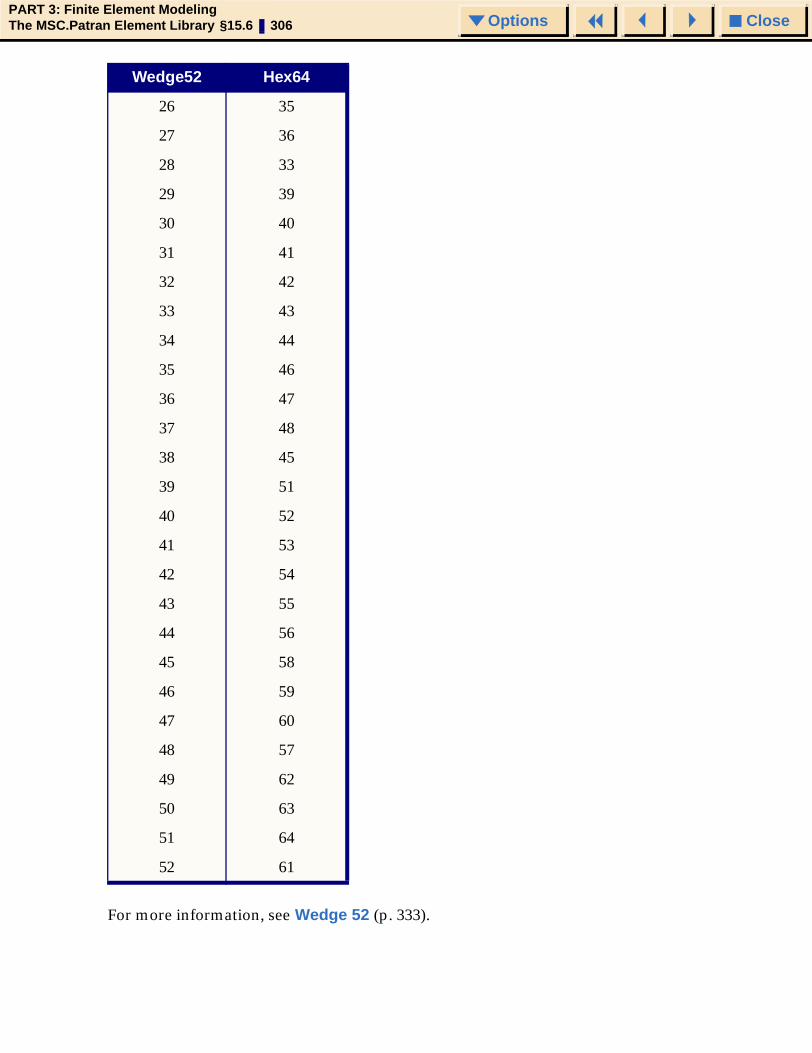
CloseOptionsPART 3: Finite Element ModelingThe MSC.Patran Element Library §15.6 306 Options
For more information, see Wedge 52 (p. 333).
26 35
27 36
28 33
29 39
30 40
31 41
32 42
33 43
34 44
35 46
36 47
37 48
38 45
39 51
40 52
41 53
42 54
43 55
44 56
45 58
46 59
47 60
48 57
49 62
50 63
51 64
52 61
Wedge52 Hex64

CloseOptionsPART 3: Finite Element ModelingThe MSC.Patran Element Library §15.7 307 Options
15.7 Hex Element TopologyMSC.Patran contains eight different hex element topologies: Hex8, Hex9, Hex20, Hex21, Hex26, Hex27, Hex32, Hex64.
General Data
Shape = Hex
Element dimensionality= 3
Number of corner nodes = 8
Number of edges = 12
Number of faces = 6
Number of face edges = 4
General Shape
TheHex parametric coordinates (Rectangular) are:
1. X axis for the Hex element is from node 1-->2.
2. Y axis for the Hex element is from node 1-->4.
3. Z axis for the Hex element is from node 1-->5.
Specific Data - Hex8
Element name = Hex8
Number of nodes = 8
Order = linear
Table 15-67 Hex Face Numbering
Face ID Sense Edge 1 Edge 2 Edge 3 Edge 4
1 1 1 2 3 4
2 -1 5 6 7 8
3 -1 1 10 5 9
4 -1 2 11 6 10
5 -1 3 12 7 11
6 -1 4 9 8 12

CloseOptionsPART 3: Finite Element ModelingThe MSC.Patran Element Library §15.7 308 Options
Degenerate element name = Wedge6
For more information, see Hex8 (p. 320).
Specific Data - Hex9
Element name = Hex9
Number of nodes = 9
Table 15-68 Hex8 Edge Numbering
Edge Number Node 1 Node 2
1 1 2
2 2 6
3 6 5
4 5 1
5 4 3
6 3 7
7 7 8
8 8 4
9 1 4
10 2 3
11 6 7
12 5 8
Table 15-69 Hex8 Node Parametric Coordinates
Node Number Xi/Eta/Zeta
1 -1.0, -1.0, -1.0
2 1.0, -1.0, -1.0
3 1.0, 1.0, -1.0
4 -1.0, 1.0, -1.0
5 -1.0, -1.0, 1.0
6 1.0, -1.0, 1.0
7 1.0, 1.0, 1.0
8 -1.0, 1.0, 1.0

CloseOptionsPART 3: Finite Element ModelingThe MSC.Patran Element Library §15.7 309 Options
Order = linear
Degenerate element name = Wedge7
For more information, see Hex9 (p. 321).
Specific Data - Hex20
Element name = Hex20
Table 15-70 Hex9 Edge Numbering
Edge Number Node 1 Node 2
1 1 2
2 2 6
3 6 5
4 5 1
5 4 3
6 3 7
7 7 8
8 8 4
9 1 4
10 2 3
11 6 7
12 5 8
Table 15-71 Hex9 Node Parametric Coordinates
Node Number Xi/Eta/Zeta
1 -1.0, -1.0, -1.0
2 1.0, -1.0, -1.0
3 1.0, 1.0, -1.0
4 -1.0, 1.0, -1.0
5 -1.0, -1.0, 1.0
6 1.0, -1.0, 1.0
7 1.0, 1.0, 1.0
8 -1.0, 1.0, 1.0
9 0.0, 0.0, 0.0

CloseOptionsPART 3: Finite Element ModelingThe MSC.Patran Element Library §15.7 310 Options
Number of nodes = 20
Order = quadratic
Degenerate element name = Wedge15
Table 15-72 Hex20 Edge Numbering
Edge Number Node 1 Node 2 Node 3
1 1 9 2
2 2 14 6
3 6 17 5
4 5 13 1
5 4 11 3
6 3 15 7
7 7 19 8
8 8 16 4
9 1 12 4
10 2 10 3
11 6 18 7
12 5 20 8
Table 15-73 Hex20 Node Parametric Coordinates
Node Number Xi/Eta/Zeta
1 -1.0, -1.0, -1.0
2 1.0, -1.0, -1.0
3 1.0, 1.0, -1.0
4 -1.0, 1.0, -1.0
5 -1.0, -1.0, 1.0
6 1.0, -1.0, 1.0
7 1.0, 1.0, 1.0
8 -1.0, 1.0, 1.0
9 0.0, -1.0, -1.0
10 1.0, 0.0, -1.0

CloseOptionsPART 3: Finite Element ModelingThe MSC.Patran Element Library §15.7 311 Options
For more information, see Hex20 (p. 322).
Specific Data - Hex21
Element name = Hex21
Number of nodes = 21
Order = quadratic
Degenerate element name = Wedge16
11 0.0, 1.0, -1.0
12 -1.0, 0.0, -1.0
13 -1.0, -1.0, 0.0
14 1.0, -1.0, 0.0
15 1.0, 1.0, 0.0
16 -1.0, 1.0, 0.0
17 0.0, -1.0, 1.0
18 1.0, 0.0, 1.0
19 0.0, 1.0, 1.0
20 -1.0, 0.0, 1.0
Table 15-74 Hex21 Edge Numbering
Edge Number Node 1 Node 2 Node 3
1 1 9 2
2 2 14 6
3 6 17 5
4 5 13 1
5 4 11 3
6 3 15 7
7 7 19 8
8 8 16 4
9 1 12 4
10 2 10 3
Table 15-73 Hex20 Node Parametric Coordinates
Node Number Xi/Eta/Zeta

CloseOptionsPART 3: Finite Element ModelingThe MSC.Patran Element Library §15.7 312 Options
For more information, see Hex21 (p. 323).
11 6 18 7
12 5 20 8
Table 15-75 Hex21 Node Parametric Coordinates
Node Number Xi/Eta/Zeta
1 -1.0, -1.0, -1.0
2 1.0, -1.0, -1.0
3 1.0, 1.0, -1.0
4 -1.0, 1.0, -1.0
5 -1.0, -1.0, 1.0
6 1.0, -1.0, 1.0
7 1.0, 1.0, 1.0
8 -1.0, 1.0, 1.0
9 0.0, -1.0, -1.0
10 1.0, 0.0, -1.0
11 0.0, 1.0, -1.0
12 -1.0, 0.0, -1.0
13 -1.0, -1.0, 0.0
14 1.0, -1.0, 0.0
15 1.0, 1.0, 0.0
16 -1.0, 1.0, 0.0
17 0.0, -1.0, 1.0
18 1.0, 0.0, 1.0
19 0.0, 1.0, 1.0
20 -1.0, 0.0, 1.0
21 0.0, 0.0, 0.0
Table 15-74 Hex21 Edge Numbering
Edge Number Node 1 Node 2 Node 3

CloseOptionsPART 3: Finite Element ModelingThe MSC.Patran Element Library §15.7 313 Options
Specific Data - Hex26
Element name = Hex26
Number of nodes = 26
Order = quadratic
Degenerate element name = Wedge20
Table 15-76 Hex26 Edge Numbering
Edge Number Node 1 Node 2 Node 3
1 1 9 2
2 2 14 6
3 6 17 5
4 5 13 1
5 4 11 3
6 3 15 7
7 7 19 8
8 8 16 4
9 1 12 4
10 2 10 3
11 6 18 7
12 5 20 8
Table 15-77 Hex26 Node Parametric Coordinates
Node Number Xi/Eta/Zeta
1 -1.0, -1.0, -1.0
2 1.0, -1.0, -1.0
3 1.0, 1.0, -1.0
4 -1.0, 1.0, -1.0
5 -1.0, 1.0, 1.0
6 1.0, -1.0, 1.0
7 1.0, 1.0, 1.0
8 -1.0, 1.0, 1.0

CloseOptionsPART 3: Finite Element ModelingThe MSC.Patran Element Library §15.7 314 Options
For more information, see Hex26 (p. 326).
Specific Data - Hex27
Element name = Hex27
Number of nodes = 27
Order = quadratic
Degenerate element name = Wedge21
9 0.0, -1.0, -1.0
10 1.0, 0.0, -1.0
11 0.0, 1.0, -1.0
12 -1.0, 0.0, -1.0
13 -1.0, -1.0, 0.0
14 1.0, -1.0, 0.0
15 1.0, 1.0, 0.0
16 -1.0, 1.0, 0.0
17 0.0, -1.0, 1.0
18 1.0, 0.0, 1.0
19 0.0, 1.0, 1.0
20 -1.0, 0.0, 1.0
21 0.0, 0.0, -1.0
22 0.0, 0.0, -1.0
23 -1.0, 0.0, 0.0
24 1.0, 0.0, 0.0
25 0.0, -1.0, 0.0
26 0.0, 1.0, 0.0
Table 15-78 Hex27 Edge Numbering
Edge Number Node 1 Node 2 Node 3
1 1 9 2
2 2 14 6
3 6 17 5
Table 15-77 Hex26 Node Parametric Coordinates
Node Number Xi/Eta/Zeta

CloseOptionsPART 3: Finite Element ModelingThe MSC.Patran Element Library §15.7 315 Options
4 5 13 1
5 4 11 3
6 3 15 7
7 7 19 8
8 8 16 4
9 1 12 4
10 2 10 3
11 6 18 7
12 5 20 8
Table 15-79 Hex27 Node Parametric Coordinates
Node Number Xi/Eta/Zeta
1 -1.0, -1.0, -1.0
2 1.0, -1.0, -1.0
3 1.0, 1.0, -1.0
4 -1.0, 1.0, -1.0
5 -1.0, -1.0, 1.0
6 1.0, -1.0, 1.0
7 1.0, 1.0, 1.0
8 -1.0, 1.0, 1.0
9 0.0, -1.0, -1.0
10 1.0, 0.0, -1.0
11 0.0, 1.0, -1.0
12 -1.0, 0.0, -1.0
13 -1.0, -1.0, 0.0
14 1.0, -1.0, 0.0
15 1.0, 1.0, 0.0
16 -1.0, 1.0, 0.0
17 0.0, -1.0, 1.0
Table 15-78 Hex27 Edge Numbering
Edge Number Node 1 Node 2 Node 3

CloseOptionsPART 3: Finite Element ModelingThe MSC.Patran Element Library §15.7 316 Options
For more information, see Hex27 (p. 329).
Specific Data - Hex32
Element name = Hex32
Number of nodes = 32
Order = cubic
Degenerate element name = Wedge24
18 1.0, 0.0, 1.0
19 0.0, 1.0, 1.0
20 -1.0, 0.0, 1.0
21 0.0, 0.0, 0.0
22 0.0, 0.0, -1.0
23 0.0, 0.0, 1.0
24 -1.0, 0.0, 0.0
25 1.0, 0.0, 0.0
26 0.0, -1.0, 0.0
27 0.0, 1.0, 0.0
Table 15-80 Hex32 Edge Numbering
Edge Number Node 1 Node 2 Node 3 Node 4
1 1 9 10 2
2 2 18 22 6
3 6 26 25 5
4 5 21 17 1
5 4 14 13 3
6 3 19 23 7
7 7 29 30 8
8 8 24 20 4
9 1 16 15 4
10 2 11 12 3
Table 15-79 Hex27 Node Parametric Coordinates
Node Number Xi/Eta/Zeta

CloseOptionsPART 3: Finite Element ModelingThe MSC.Patran Element Library §15.7 317 Options
For more information, see Hex32 (p. 330).
Specific Data - Hex64
Element name = Hex64
Number of nodes = 64
Order = cubic
11 6 27 28 7
12 5 32 31 8
Table 15-81 Hex32 Node Parametric Coordinates
Node Number Xi/Eta/Zeta Node Number Xi/Eta/Zeta
1 -1.0, -1.0, -1.0 17 -1.0, -1.0, -1/3
2 1.0, -1.0, -1.0 18 1.0, -1.0, -1/3
3 1.0, 1.0, -1.0 19 1.0, 1.0, -1/3
4 -1.0, 1.0, -1.0 20 -1.0, 1.0, -1/3
5 -1.0, -1.0, 1.0 21 -1.0, -1.0, 1/3
6 1.0, -1.0, 1.0 22 1.0, -1.0, 1/3
7 1.0, 1.0, 1.0 23 1.0, 1.0, 1/3
8 -1.0, 1.0, 1.0 24 -1.0, 1.0, 1/3
9 -1/3, -1.0, -1.0 25 -1/3, -1.0, 1.0
10 1/3, -1.0, -1.0 26 1/3, -1.0, 1.0
11 1.0, -1/3, -1.0 27 1.0, -1/3, 1.0
12 1.0, 1/3, -1.0 28 1.0, 1/3, 1.0
13 1/3, 1.0, -1.0 29 1/3, 1.0, 1.0
14 -1/3, 1.0, -1.0 30 -1/3, 1.0, 1.0
15 -1.0, 1/3, -1.0 31 -1.0, 1/3, 1.0
16 -1.0, -1/3, -1.0 32 -1.0, -1/3, 1.0
Table 15-80 Hex32 Edge Numbering
Edge Number Node 1 Node 2 Node 3 Node 4

CloseOptionsPART 3: Finite Element ModelingThe MSC.Patran Element Library §15.7 318 Options
Degenerate element name = Wedge52
Table 15-82 Hex64 Edge Numbering
Edge Number Node 1 Node 2 Node 3 Node 4
1 1 9 10 2
2 2 18 22 6
3 6 26 25 5
4 5 21 17 1
5 4 14 13 3
6 3 19 23 7
7 7 29 30 8
8 8 24 20 4
9 1 16 15 4
10 2 11 12 3
11 6 27 28 7
12 5 32 31 8
Table 15-83 Hex64 Node Parametric Coordinates
Node Number Xi/Eta/Zeta Node
Number Xi/Eta/Zeta Node Number Xi/Eta/Zeta
1 -1.0, -1.0, -1.0 23 1.0, 1.0, 1/3 45 -1/3, -1/3, -1/3
2 1.0, -1.0, -1.0 24 -1.0, 1.0, 1/3 46 1/3, -1/3, -1/3
3 1.0, 1.0, -1.0 25 -1/3, -1.0, 1.0 47 1/3, 1/3, -1/3
4 -1.0, 1.0, -1.0 26 1/3, -1.0, 1.0 48 -1/3, 1/3, -1/3
5 -1.0, -1.0, 1.0 27 1.0, -1/3, 1.0 49 -1/3, -1.0, 1/3
6 1.0, -1.0, 1.0 28 1.0, 1/3, 1.0 50 1/3, -1.0, 1/3
7 1.0, 1.0, 1.0 29 1/3, 1.0, 1.0 51 1.0, -1/3, 1/3
8 -1.0, 1.0, 1.0 30 -1/3, 1.0, 1.0 52 1.0, 1/3, 1/3
9 -1/3, -1.0, -1.0 31 -1.0, 1/3, 1.0 53 1/3, 1.0, 1/3
10 1/3, -1.0, -1.0 32 -1.0, -1/3, -1.0 54 -1/3, 1.0, 1/3
11 1.0, -1/3, -1.0 33 -1/3, -1/3, -1.0 55 -1.0, 1/3, 1/3
12 1.0, 1/3, -1.0 34 1/3, -1/3, -1.0 56 -1.0, -1/3, 1/3
13 1/3, 1.0, -1.0 35 1/3, 1/3, -1.0 57 -1/3, -1/3, 1/3

CloseOptionsPART 3: Finite Element ModelingThe MSC.Patran Element Library §15.7 319 Options
For more information, see Hex64 (p. 334).
14 -1/3, 1.0, -1.0 36 -1/3, 1/3, -1.0 58 1/3, -1/3, 1/3
15 -1.0,1/3, -1.0 37 -1/3, -1.0, -1/3 59 1/3, 1/3, 1/3
16 -1.0, -1/3, -1.0 38 1/3, -1.0, -1/3 60 -1/3, 1/3, 1/3
17 -1.0, -1.0, -1/3 39 1.0, -1/3, -1/3 61 -1/3, -1/3, 1.0
18 1.0, -1.0, -1/3 40 1.0, 1/3, -1/3 62 1/3, -1/3, 1.0
19 1.0, 1.0, -1/3 41 1/3, 1.0, -1/3 63 1/3, 1/3, 1.0
20 -1.0, 1.0, -1/3 42 -1/3, 1.0, -1/3 64 -1/3, 1/3, 1.0
21 -1.0, -1.0, 1/3 43 -1.0, 1/3, -1/3
22 1.0, -1.0, 1/3 44 -1.0, -1/3, -1/3
Table 15-83 Hex64 Node Parametric Coordinates
Node Number Xi/Eta/Zeta Node
Number Xi/Eta/Zeta Node Number Xi/Eta/Zeta

CloseOptionsPART 3: Finite Element ModelingThe MSC.Patran Element Library §15.8 320 Options
15.8 MSC.Patran’s Element Library
21
1 2
3
1 2
34
1
2
3
4
6
5
2
3
1
4
8
7
6
2
3
1
54
Bar2 Tri3
Tet4
Hex8Wedge 6
Quad4

CloseOptionsPART 3: Finite Element ModelingThe MSC.Patran Element Library §15.8 321 Options
1 2
3
1
23
4
1
2
3
45
5
4 3
21
4
6
5
7
8
5
4
7
3
2
9
1
6
Quad5 Tri4
Wedge7Tet5
Hex9

CloseOptionsPART 3: Finite Element ModelingThe MSC.Patran Element Library §15.8 322 Options
21
1 2
3
1 2
34
1
6
5
2
3
1
4
4
98
73
6
5 2
15
14
813
7
9
187
19
8 15
9
2
112
4
16
20
115
13
10
14
6
317
6
5
4
7
5
10
Bar3 Tri6
Tet10Quad8
Wedge15 Hex20
10
12
11
68
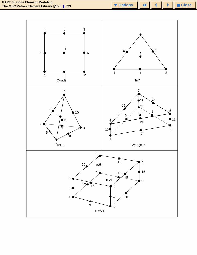
CloseOptionsPART 3: Finite Element ModelingThe MSC.Patran Element Library §15.8 323 Options
1 2
3
1
2
3
4
1
2
3
4
5
9
4 3
21
7
6
5
7
8
5
4
7
3
2
21
1
6
6
7
8
5
5
4
6
6
7
8
9
10
11 11
1412
15
9
10
13
816
13
14
15
1620
12 17
9
18
10
19
11
Quad9
Tet11
Hex21
Wedge16
Tri7

CloseOptionsPART 3: Finite Element ModelingThe MSC.Patran Element Library §15.8 324 Options
SURFACE NODES
SURFACE NODES
6
3
1114
13
1
5
2
9
4 10
8 7
y
x
z
2
9
43
6
10
12
y
x
z
Tet14

CloseOptionsPART 3: Finite Element ModelingThe MSC.Patran Element Library §15.8 325 Options
1
9
3
8
2
7 16
y
x z
19
12
18
11
20
y
x z
10
4
15
6
14
5
13 17
y
x z
6
12
3
4
10
1
5
13
15
14
7 8
2
LEVEL 3
LEVEL 2
LEVEL 1
x
z
y
LEVEL 1 LEVEL2
LEVEL3
11
Wedge20
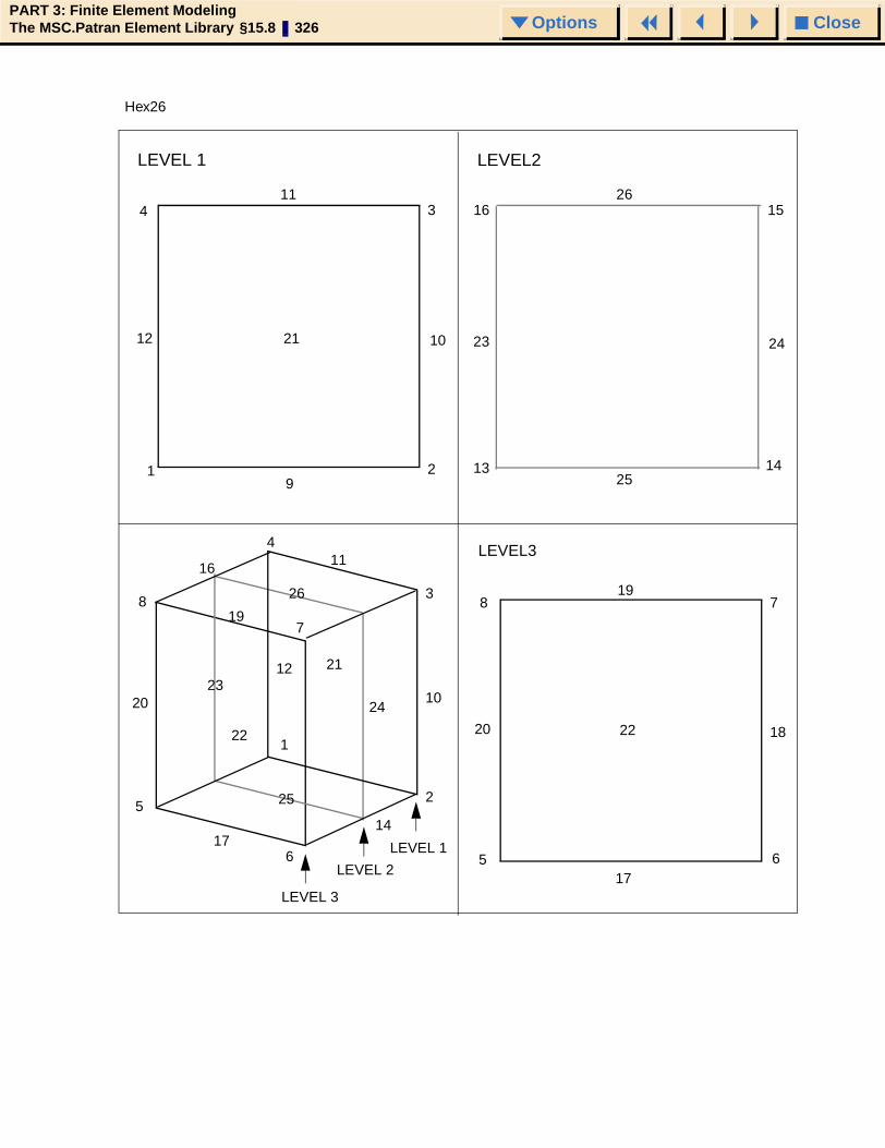
CloseOptionsPART 3: Finite Element ModelingThe MSC.Patran Element Library §15.8 326 Options
10
1
12
LEVEL 1 LEVEL2
LEVEL3
411
3
2
21
9
1626
15
24
1425
13
23
8
20
5
19
17
7
18
6
22
8
20
5
16
411
3
10
2
14
617
24
26
23
25
12
1
7
22
21
19
LEVEL 3
LEVEL 2
LEVEL 1
Hex26

CloseOptionsPART 3: Finite Element ModelingThe MSC.Patran Element Library §15.8 327 Options
LEVEL 1 LEVEL 2
LEVEL 3
Z
X
Y Y
X
Z
Y
Z X
Y
X
2
4 310
148 7
5
115 12
9 6
2
410
3
6 9
13
2
4 1
11
2
431
11
Tet15

CloseOptionsPART 3: Finite Element ModelingThe MSC.Patran Element Library §15.8 328 Options
1
9
3
8
2
7 17
y
x z
20
12
19
11
21 16
y
x z
10
4
15
6
14
5
13 18
y
x z
6
12
3
4
10
1
5
13
15
14
7 8
2
LEVEL 3
LEVEL 2
LEVEL 1
x
z
y
LEVEL 1 LEVEL 2
LEVEL 3
21 19
Wedge21

CloseOptionsPART 3: Finite Element ModelingThe MSC.Patran Element Library §15.8 329 Options
10
1
12
LEVEL 1 LEVEL 2
LEVEL 3
411
3
2
22
9
1627
15
25
1426
13
24
8
20
5
19
17
7
18
6
23
8
20
5
16
411
3
10
2
14
617
25
27
24
25
12
1
7
23
22
19
LEVEL 3
LEVEL 2
LEVEL 1
21
139
15
Hex27

CloseOptionsPART 3: Finite Element ModelingThe MSC.Patran Element Library §15.8 330 Options
21
1 2
3
1 2
34
1
6
5
2
3
1
4
4
9 87
3
65 2
23
7
19
7
8
9
2
1
154
20
5 18
6
3
3 4 9
87
6
54
10
11
14 15
12
13
1611
12
10 9
8
7
65
16
10
22
2728
29
30
31 32
1314
1923
24
26
1112
25
8
1417
21
22
24
20
1613
1815
10
9
11
12
21
17
Bar4 Tri9
Tet16Quad12
Wedge24 Hex32

CloseOptionsPART 3: Finite Element ModelingThe MSC.Patran Element Library §15.8 331 Options
2
3
14 5
6
78
9
12
1113
10
4 10 9 3
11
12
1 5 6 2
8
7
1516
1413
Quad16
Tri13
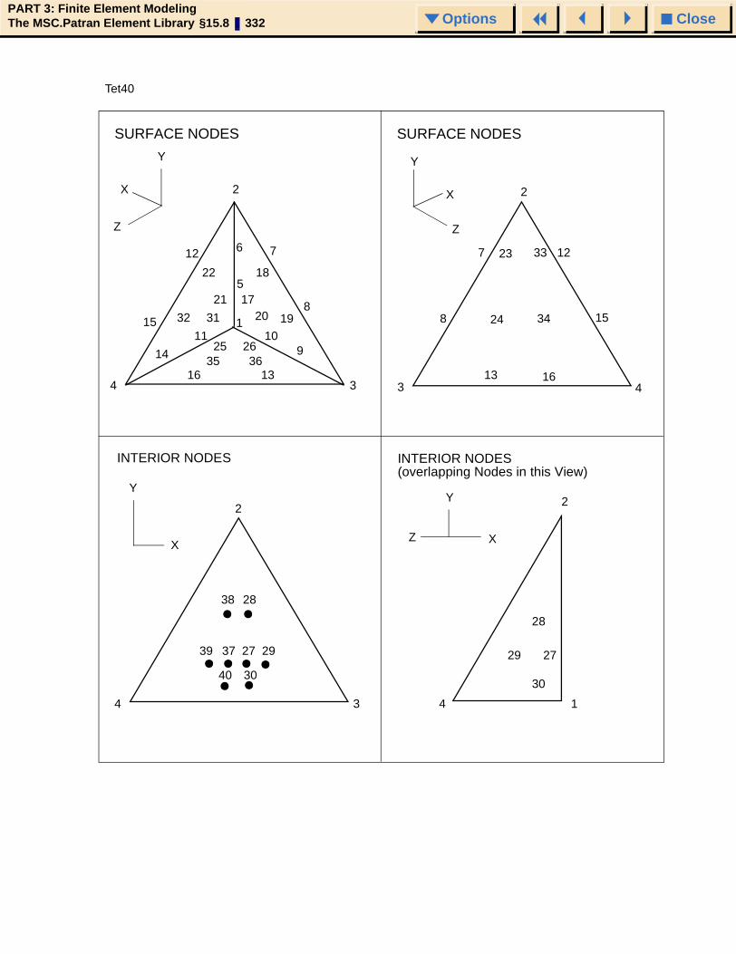
CloseOptionsPART 3: Finite Element ModelingThe MSC.Patran Element Library §15.8 332 Options
SURFACE NODES SURFACE NODES
INTERIOR NODES
Z
X
Y Y
X
Z
Y
Z X
Y
X
2
4 3
1
2
43
2
4 1
2
34
(overlapping Nodes in this View) INTERIOR NODES
16 1335 36
25 2610
914
11
32 31 20 19
21 175
6
22 18
7
8
12
15
7 23 33 12
8 24 34 15
13 16
30
28
29 27
38 28
39 37 27 29
40 30
Tet40
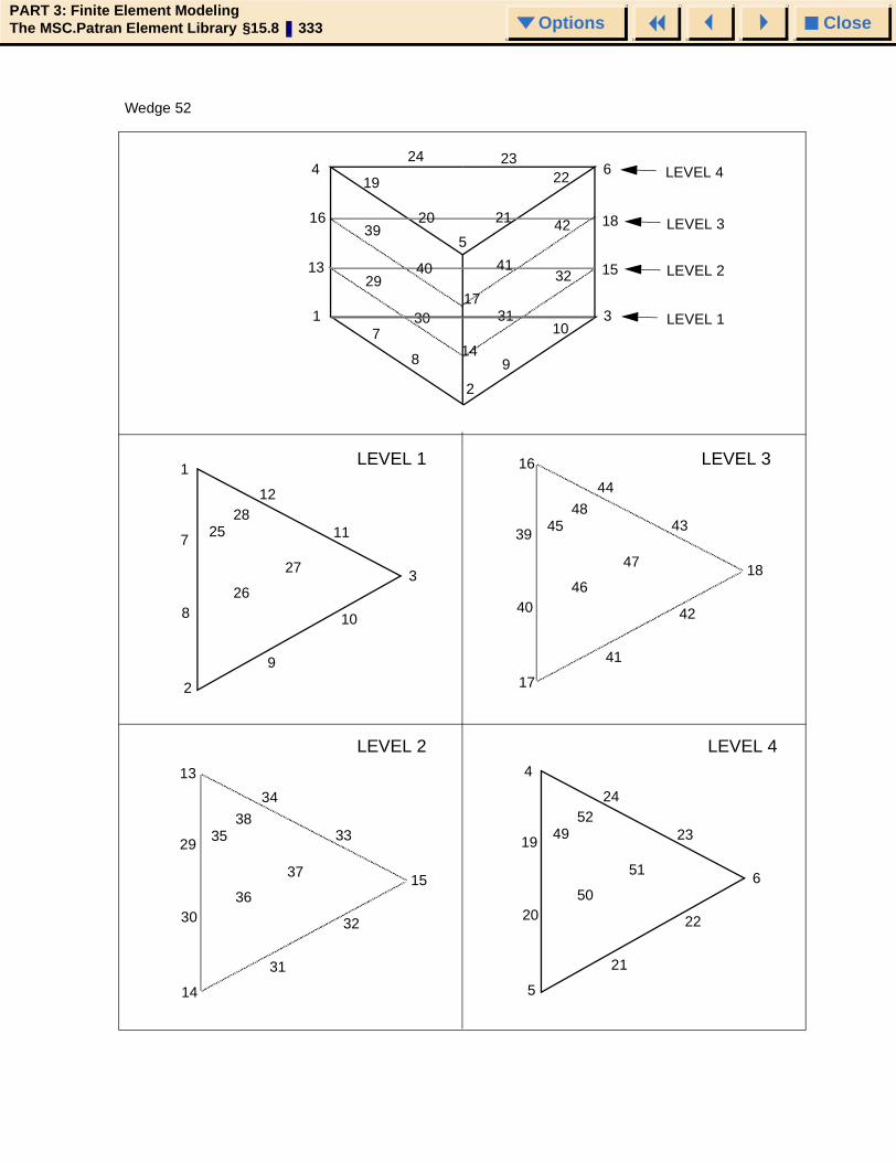
CloseOptionsPART 3: Finite Element ModelingThe MSC.Patran Element Library §15.8 333 Options
4
16
13
1
6
18
15
3
24 23
19
39
29
7
20
40
30
8
21
41
31
9
22
42
32
10
5
17
14
2
1
7
8
2
12
11
3
10
9
2528
27
26
16
39
40
17
44
43
18
42
41
4548
47
46
13
29
30
14
34
33
15
32
31
3538
37
36
4
19
20
5
24
23
6
22
21
4952
51
50
LEVEL 1 LEVEL 3
LEVEL 2 LEVEL 4
LEVEL 4
LEVEL 3
LEVEL 2
LEVEL 1
Wedge 52
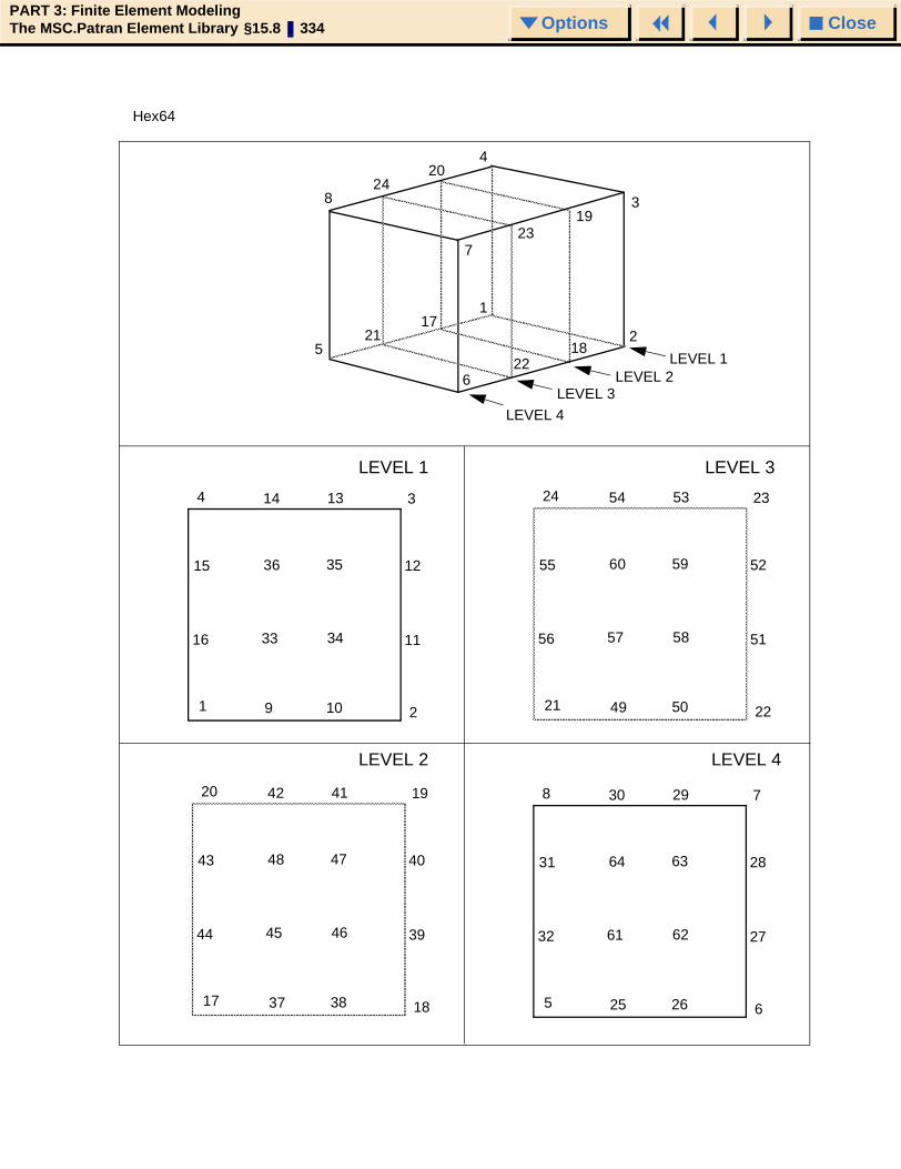
CloseOptionsPART 3: Finite Element ModelingThe MSC.Patran Element Library §15.8 334 Options
LEVEL 1 LEVEL 3
LEVEL 2 LEVEL 4
8
31
32
5
30
64
61
25
29
63
62
26
7
28
27
6
4
15
16
1
14
36
33
9
13
35
34
10
3
12
11
2
20
43
44
17
42
48
45
37
41
47
46
38
19
40
39
18
24
55
56
21
54
60
57
49
53
59
58
50
23
52
51
22
824
204
723
193
218
226
521
171
LEVEL 4
LEVEL 3 LEVEL 2
LEVEL 1
Hex64

O Q C A B D E F G H I J K L M N P R S T U V W X Y Z#
I N D E XMSC.Patran Reference Manual Part 3: Finite Element Modeling
CloseOptionsMSC.Patran Reference ManualIndex 335 Options
I N D E XMSC.Patran Reference Manual
Part 3: Finite Element Modeling
Aaccess finite element modeling, 5analysis coordinate frame, 2any, 248arc method, 82aspect ratio, 187associate, 9
curve, 111node, 114point, 110solid, 113surface, 112
associate action, 109attributes, 2Auto TetMesh, 8
Bbars, 228building finite element model, 6
Ccollapse, 195connectivity, 2constraint, 2create
mesh seeding, 19meshing curves, 14meshing solids, 17meshing surfaces, 15remeshing/reseeding, 21
create action, 12creating finite element model, 8curve method, 111cyclic symmetry, 2, 62
Ddegrees-of-freedom, 2, 57
delete, 9any, 248DOF List, 258element, 255mesh control, 253mesh curve, 251mesh seed, 249mesh solid, 252mesh surface, 250MPCs, 256node, 254superelement, 257
delete action, 247dependent DOF, 2disassociate, 117
elements, 118node, 119
disassociate action, 117
Eedge angle, 193edit, 225editing, 8element, 255
boundaries, 140connectivity, 143duplicates, 141IDs, 147Jacobian Ratio, 145Jacobian Zero, 146normals, 142
element attributes, 203element coordinate system, 205element topology, 13element-element
geometry fit, 144elements, 76, 77, 78, 105, 132
mirror, 78renumber, 105rotate, 77translate, 76

O Q C A B D E F G H I J K L M N P R S T U V W X Y Z#
I N D E XMSC.Patran Reference Manual Part 3: Finite Element Modeling
CloseOptionsMSC.Patran Reference ManualIndex 336 Options
equivalenceall, 125group, 126list, 127
equivalence action, 122equivalencing, 2, 9examples, 260explicit, 2extrude method, 83
FFEM data, 97finite element, 2finite element model, 2free edges, 2free faces, 2
Gglide control, 85glide method, 84glide-guide control, 88glide-guide method, 86graphics, 58group, 126
Hhex
all, 172aspect, 174edge angle, 175face skew, 176face taper, 179face warp, 177twist, 178
Iimplicit, 2
independent DOF, 2IsoMesh, 2, 8, 15
2 curve, 39curve, 38surface, 40
JJacobian Ratio, 3Jacobian Zero, 3
Llibrary, 3list, 127loft method, 96
Mmesh, 214mesh control, 49, 253mesh control data, 98mesh curve, 251mesh paths, 15, 17mesh seed, 30, 222, 249
curvature based, 33one way bias, 31tabular, 34two way bias, 32uniform, 30
mesh seed attributes, 206mesh seeding, 19mesh solid, 252mesh surface, 250mesh transitions, 19meshing curves, 14meshing solids, 17meshing surfaces, 15midnode
normal offset, 181tangent offset, 182

O Q C A B D E F G H I J K L M N P R S T U V W X Y Z#
I N D E XMSC.Patran Reference Manual Part 3: Finite Element Modeling
CloseOptionsMSC.Patran Reference ManualIndex 337 Options
modify, 9bars, 228edit, 225mesh, 214mesh seed, 222MPCs, 242nodes, 238quads, 233trais, 229
modify action, 213MPC, 3, 208
cyclic symmetry, 62degrees-of-freedom, 57graphics, 58sliding surface, 63
MPC create, 9MPC terms, 57MPC types, 56, 60MPCs, 56, 242, 256multiple MPCs, 58
Nnode, 254
IDs, 180node distance, 202node location, 201nodes, 54, 71, 72, 74, 104, 132, 238
mirror, 74renumber, 104rotate, 72translate, 71
non-uniform seed, 3normal method, 89normals, 3
Ooptimization, 3optimization method, 133optimize, 9
nodes/elements, 132
optimize action, 130
Pparameters, 3paths, 3paver, 3, 8, 15point method, 110
Qquad, 233
all, 152aspect, 154skew, 156taper, 157warp, 155
Rradial cylindrical method, 90radial spherical method, 91reference coordinate frame, 3remeshing/reseeding, 21renumber, 3, 9
action, 103rezoning, 97
Sseeding, 3seeding solid, 19seeding surface, 19shape, 3

O Q C A B D E F G H I J K L M N P R S T U V W X Y Z#
I N D E XMSC.Patran Reference Manual Part 3: Finite Element Modeling
CloseOptionsMSC.Patran Reference ManualIndex 338 Options
show, 9element attributes, 203element coordinate system, 205mesh control attributes, 207mesh seed attributes, 206MPC, 208node distance, 202node location, 201
show action, 200skew, 184sliding surface, 3, 63solid
IsoMesh, 42TetMesh, 45
solid method, 113spherical theta method, 92sub MPC, 3surface method, 112sweep, 9
arc, 82extrude, 83glide, 84glide-guide, 86loft, 96normal, 89radial cylindrical, 90radial spherical, 91spherical theta, 92vector field, 94
sweep action, 81
Ttaper, 192term, 3Tet
all, 158aspect, 160collapse, 163edge angle, 161face skew, 162
TetMesh, 4, 8parameters, 47
theory, 184aspect ratio, 187collapse, 195edge angle, 193skew, 184taper, 192twist, 196warp, 191
topology, 4transform, 9transform action, 70transitions, 4tria
all, 148aspect, 150skew, 151
triangular elements, 19trias, 229twist, 196types, 4
Uuniform seed, 4
Vvector field method, 94verification, 4, 9

O Q C A B D E F G H I J K L M N P R S T U V W X Y Z#
I N D E XMSC.Patran Reference Manual Part 3: Finite Element Modeling
CloseOptionsMSC.Patran Reference ManualIndex 339 Options
verifyelement
boundaries, 140connectivity, 143duplicates, 141IDs, 147Jacobian Ratio, 145Jacobian Zero, 146normals, 142
element-elementgeometry fit, 144
hexall, 172aspect, 174edge angle, 175face skew, 176face taper, 179face warp, 177twist, 178
midnodenormal offset, 181tangent offset, 182
nodeIDs, 180
quadall, 152aspect, 154skew, 156taper, 157warp, 155
Tetall, 158aspect, 160collapse, 163edge angle, 161face skew, 162
triaall, 148aspect, 150skew, 151
wedgeall, 164aspect, 166
edge angle, 167face skew, 168face taper, 171face warp, 169twist, 170
verify action, 136
Wwarp, 191wedge
all, 164aspect, 166edge angle, 167face skew, 168face taper, 171face warp, 169twist, 170