msc in geology
TRANSCRIPT

UNIVERSITY OF NAIROBI
DEPARTMENT OF GEOLOGY
MSc IN GEOLOGY
nSSUBSURFACE STRUCTURES AND CHARACTERIZATION OF THE SILALI
GEOTHERMAL SYSTEM, KENYA RIFT. / r
By
Kangogo Deflorah Jerobon
Reg No: 156/77008/09
University of NAIROBI Library
0439129 8
A dissertation submitted to the University of Nairobi in partial fulfillment of the
requirements for the Degree of Master of Science in Geology (Applied Geophysics).
2011
f

DECLARATION
I certify that although I may have conferred with others in preparing for this assignment, and
drawn upon a range o f sources cited in this work, the content of this thesis report is my original
work and has not been presented for a degree in any other university or any other award.
Signature _________ Date:
Deflorah Kangogo
1 confirm that the candidate under our supervision has undertaken the work in this dissertation
report.
Prof. Justus Barongo
Department of Geology, University o f Nairobi.

ABSTRACT
Electrical resistivity methods are widely applied in geothermal exploration and are the cheapest
means of acquiring subsurface data. Further detailed surveys like exploratory drilling which is
cost intensive in an area under study is always based on accurate surface exploration results.
Several exploration methods are applicable in geophysical prospecting o f geothermal resources;
however, this study focuses mainly on application o f electromagnetic methods namely Transient
Electromagnetic (TEM) and Magnetotelluric (MT). During the detailed exploration surveys of
Silali geothermal prospect situated in the floor of the Northern Kenya rift, MT and TEM methods
were applied. The survey was to map out the subsurface resistivity, which is then interpreted so
as to provide information such as fluid filled fractures, the reservoir and the heat source. Joint
one dimensional (1-D) inversions of MT and TEM data were done so as to correct for static shift
in MT soundings. Results of the joint 1-D inversion o f MT and TEM data revealed four main
resistivity zones; A shallow high resistivity zone (> 100 ftm) to about 300 m below the surface
which is as a result of unaltered rocks, 2) An intermediate low resistivity zone (10 f2m) to
depths of about I km which is as a result of low temperature hydrothermal alteration minerals, 3)
A deeper high resistivity (> 50 Om), up to 3-4 km depth indicating high temperature minerals
occurring at depth. The shallow boundary between an upper, low resistive layer and the
underlying intermediate resistivity zone at depths of 800-3500 m appears to mark the change in
clay mineralogy from low grade alteration mineralogy represented by smectite to high grade
alteration mineralogy represented by chlorite, epidote and actinolite, which is interpreted as the
geothermal reservoir zone of this study area, and 4) a deeper low resistivity region, at a depth of
about 5000 m below sea level is inferred to be magmatic material or intrusion i.e., the heat
source o f this study area. The resultant 2-D resistivity models showed significant variations in
the resistivity distribution both vertically and horizontally on all profiles indicating major
structural controls o f the geothermal system. This study concludes that a geothermal resource
exists in Silali caldera and the nearly vertical conductors in the resistive zones are fluid filled
fracture systems/faults and are best targets for exploratory drilling. It is, therefore, recommended
that deep exploration wells be drilled within the caldera floor and outside the caldera to the east
to further confirm the nature and potential of the resource at Silali.
n

ACKNOW LEDGEMENT
I wish to express my gratitude to my God for giving me health and insights throughout the
project period. Thanks to entire University o f Nairobi fraternity more so to my supervisor
Professor Justus Barongo for guiding me through the process by constructive criticism and
advice. Many thanks go to Mr. James Wambugu Manager, Resource Development, Geothermal
Development Company (GDC) and Mr. John Lagat, C hief Geologist, GDC for ensuring success
in this research. Many thanks go to Charles Muturia, Senior Geophysicist, GDC for training me
on the data collection, processing, analysis and interpretation ensuring overall success in my
project objectives.
I am also greatly indebted to the staff at the University o f Nairobi, Department o f Geology and
GDC for contributing in their own unique ways towards this project. Finally many thanks to my
parents Mr. and Mrs. Kegei for guiding me and always installing hope and patience in my
academic life.
m

t a b l e o f c o n t e n t s
d e c l a r a t io n ..............................................................................................................................
ABSTRACT...................................................................................................................................... i
ACKNOWLEDGEMENT..............................................................................................................ii
List of Figures.................................................................................................................................vi
List of Tables................ vii
List of Plates...................................................................................................................................vii
Acronyms......................................................................................................................................... i>
CHAPTER O N E............................................................................................................................... 1
1.0 INTRODUCTION.......................................................................................................................1
1.1 Problem statement.................................................................................................................. 3
1.2 Research motivation............................................................................................................... 5
1.3 Aim and objectives................................................................................................................. 5
1.3.1 Specific objectives............................................................................................................... 5
1.3.2 Justification and significance.............................................................................................. 5
1.4 Literature review..................................................................................................................... 6
1.4.1 Seismology...........................................................................................................................7
1.4.2 Gravity and ground magnetics........................................................................................... 8
1.5 Application of resistivity methods in geothermal exploration........................................ 12
1.6 The role of electrical resistivity..........................................................................................12
1.7 Resistivity of rocks............................................................................... ;............................. 14
1.8 Salinity of water................................................................................................................... 15
1.9 Temperature........................................................................................................................... 16
1.10 Pressure................................................................................................................................ 17
1.11 Porosity and permeability of a rock................................................................................. 18
1.12 Water-rock interaction and alteration................................................................................19
CHAPTER TWO.............................................................................................................................21
2.0 REGIONAL AND LOCAL SETTING OF THE STUDY AREA....................................... 21
2.1 Introduction...........................................................................................................................21
2.2 Location.................................................................................................................................23
2.3 Physiography and drainage.................................................................................................. 23
2.3.1 Physiography.......... .........................................., .......*.............. ......'................................ 23

2.3.2 Drainage........................................................................................................................... 23
2.4 Topography............................................................................................................................25
2.5 Climate...................................................................................................................................25
2.6 Vegetation..............................................................................................................................25
2.7 Land use and land resources................................................................................................ 26
2.8 Geology of the study area.................................................................................................. 26
2.8.1 Structural setting of Silali................................................................................................. 28
2.8.2 Geothermal manifestations............................................................................................... 30
2.8.3 Hydrogeology.................................................................................................................... 32
2.8.4 The potentiometric map and regional flow patterns......................................................32
CHAPTER THREE........................................................................................................................ 35
3.0 BASIC PRINCIPLES OF THE METHODS USED............................................................. 35
3.1 General introduction.............................................................................................................35
3.2 Basic theory for Transient Electromagnetics (TEM) Method.......................................... 35
3.4 Basic theory of magneto-telluric method (MT)................................................................40
3.5 Electromagnetic induction in a homogenous earth............................................................ 42
3.6 Skin depth..............................................................................................................................44
3.7 MT dead band....................................................................................................................... 44
CHAPTER FOUR...........................................................................................................................45
4.0 DATA AQUISITION AND PROCESSING OF DATA......................................................45
4.1 Brief Outline......................................................................................................................... 45
4.2 Research Design................................................................................... :............................. 45
4.3 Field Instrumentation......................................................................................' ................... 48
4.3.1 Magnetotelluric (MT) method..........................................................................................48
4.3.2 Transient Electromagnetic (TEM) method......................................................................49
4.4 Field Data Acquisition and Processing............................................................................... 51
4.4.1 Magnetotelluric (MT) field survey.................................................................................. 51
4.4.2 Transient Electromagnetic (TEM) field survey............................................................. 52
4.4.3 Data processing......................................................................' ..........................................52
4.4.3.1 General introduction.......................................................................................................52
4.4.3.2 Magnetotelluric (MT) static shift correction using Transient Electromagnetic (TEM)...................................................................................................................................................... 53
CHAPTER FIVE.................. >.....................................................................-................................ 55/
v

5 0 DATA ANALYSIS AND DISCUSSION OF RESULTS...................................................55
5.1 Introduction........................................................................................................................................55
5 2 One dimension (ID) inversion and interpretation............................................................ 55
5 3 Two dimension (2D) inversion and interpretation.......................................................... 61
5.3.1 The east-west oriented profile lines..................................................................................63
5 3.2 The North-South oriented profile lines........................................................................... 66
5 3.3 The northwest-southeast oriented profile lines................................................................67
5.3.4 The southwest-northeast oriented profile lines................................................................69
5.4 Conceptualized Geothermal Model...................................................................................72
5.4.1 Silali Hydrothermal System............................................................................................. 72
5.4.2 Heat source.........................................................................................................................72
5.4.3 Recharge and permeability............................................................................................... 72
5.4.4 System capping:................................................................................................................. 73
5.4.5 Geothermal System............................................................................................................73
CHAPTER SIX...............................................................................................................................75
6.0 CONCLUSIONS AND RECOMMENDATIONS.............................................................. 75
REFERENCES................................................................................................................................77
APPENDIX I: STATIC SHIFT CORRECTION OF MT USING TEM....................................83
/VI

List of Figures
Figure 1.1: Map showing the Kenya rift and the volcanic centers................................................2
Figure 1.2. Seismicity distribution in Kenya from temporary local networks............................. 9
Figure 1.3. Band-pass filtered gravity map of the northern part of the Kenya rift.....................10
Figure 1.4. Aeromagnetic residual field intensity contour map................................................. 11
Figure 1.5: Alteration mineralogy with increasing temperature in basaltic country rock........13
Figure 1.6: Schema of a generalised geothermal system..............................................................14
Figure 1.7: Pore fluid conductivity vs. salinity for a variety of electrolytes.............................. 16
Figure 1.8: Electrical resistivity of water as a function of temperature at different pressures. 17
Figure 1.9: General resistivity structure of high temperature geothermal field........................ 20
Figure 2.1: Map of the Kenya rift showing Silali and other northern rift sector volcanoes.... 22
Figure 2.2: The map of the drainage system in the study area....................................................24
Figure 2.3: Simplified geological and structural map of Silali volcano..................................... 27
Figure 2.4: Tectonics of the Silali region...................................................................................... 29
Figure 2.5 Map showing the geothermal manifestations in the Silali geothermal prospect.... 31
Figure 2.6: The potentiometric map between Lake Baringo and Lake Turkana...................... 34
Figure 3.1: The central loop TEM configuration.........................................................................37
Figure 3.2: Basic principles of the TEM method..........................................................................38
Figure 3.3: Voltage response for homogenous half space.......................................................... 39
Figure 3.4: Late time apparent resistivity for homogenous half space......................................40
Figure 3.5: MT-soundings layout.................................................................... 41
Figure 3.6: Homogenous half space response of electric and magnetic field........ ....................43
Figure 4.1: A schematic illustration of the approach used for during research project.............47
Figure 4.2: V5 System 2000 (MTU series).................................................................................. 48
Figure 4.3: Zonge TEM transmitter.............................................................................................. 49
Figure 4.4: Three phase generator................................................................................................. 49
Figure 4.5: Transmitter controllers................................................................................................ 50
Figure 4.6: GDP-32 receiver............................................................... 50
Figure 5.1: One-dimensional Occam resistivity inversion models............................................. 57
Figure 5.2: Resistivity at 500 m above sea level.......................................................................... 58
Figure 5.3: Resistivity at sea level................................................................................................ 59
Figure 5.4: Resistivity at 2000, m below sea level................ 60
Figure 5.5: Resistivity at 5000 m below sea level......... ......................... i....:............................. 61

Figure 5.6: Silali contour map showing the sounding points.....................................................62
Figure 5.7: Two-dimensional resistivity cross-section along E-W Line 1.............. 64
Figure 5.8: Two-dimensional resistivity cross-section along E-W Line 2 ............. 65
Figure 5.9: Two-dimensional resistivity cross-section along E-W Line 3..............65
Figure 5.10:Two-dimensional resistivity cross-section along the north-south profile..............66
Figure 5.11 :Two-dimensional resistivity cross-section along the north-south profile line 5... 67
Figure 5.12: Two-dimensional resistivity models of the northwest-southeast profiles............68
Figure 5.13: Two-dimensional resistivity models of the northwest-southeast Line7...............68
Figure 5.14: Two-dimensional Resistivity cross-section along N W-SE Line 8........................ 69
Figure 5.15: The E-W conceptualised geothermal model of Silali caldera...............................74
Figure 6.1: Resistivity anomaly map at 5000 mbsl showing the proposed wells...................... 76
List of Tables
Table 1: Stratigraphy and evolution of the Silali volcano......................................................... 28
List of Plates
Plate 1: The general physiography of Silali caldera....................................................................23
/
Vlll

A cron ym s
a f r e p r e n African Energy Policy Research Network
ASAL Arid and Semi-Arid Lands
EM Electromagnetic
gu Gravity Unit
GDC Geothermal Development Company
GoK Government of Kenya
ISOR Iceland GeoSurvey
Ka Kilo annum
KenGen Kenya Electricity Generating Company
KNBS Kenya National Bureau of Statistics
KPLC Kenya Power and Lighting Company
KRV Kenya Rift Valley
Ma Mega annum
MoE Ministry of Energy
MT Magnetotelluric
MW Mega Watt
TEM Transient Electromagnetic
/IX

I
CHAPTER ONE
1.0 INTRODUCTION
Silali geothermal prospect, herein referred to as the study area, is the largest and the
most spectacular trachytic caldera volcano in the axis of the northern Kenya Rift Valley
(KRV). It is a broad, low angle shield, with an elliptical shape slightly elongated in a N-
S direction (Figure 1.1). The volcanic shield covers an area of about 900 km2 and rises
to 760 m above the rift floor. The summit of the volcano is at 1528 masl and is
occupied by a caldera that measures 7.5 km by 5 km and is bounded by 300 m cliffs.
The latest activity from a satellite vent on the northern slopes of Silali is basaltic in
composition and to the east is trachytic in composition and was erupted about 200-300
years ago. The young activity associated with the volcano indicates that the magmatic
body under the volcano is still hot and able to sustain a geothermal system. This means
that there is a remarkable geothermal potential in the region and therefore presents an
opportunity for major geothermal power developments in the region which requires
geophysical exploration for detailed mapping of the subsurface structure and
characterization of the geothermal system.
In the past few decades, application of geo-electrical methods in geothermal
prospecting has proven to be a powerful tool. The use of electromagnetic (EM)
resistivity methods has become increasingly more effective in characterizing and
delineating potential geothermal reservoirs to an extent that even prospects with no
surface manifestations have been resolved and delineated. Resistivity methods
determine the variations in electrical resistivity of the subsurface both laterally and with
depth. Therefore, methods such as (MT) and (TEM) based on the principles of naturally
varying magnetic field and controlled magnetic field source techniques, respectively,
have been used in this study in mapping the subsurface structure.
1i

j / Emuruangogolak - j - S i l a l i
Menengai
Lake Baringo Lake Bogoria K e n ya
T^ P v« (C\V ic t o r ia ^ ^ ^ — <Lake Nakuru^ x Lake Elmentaita
! / ' / __Eburru ^ Lake Naivashai / X Eburru Lake NaivashaOlkaria--------^ \ Longonot
— — 35-y ^ // V Suswa
" ? a , e . C V . /_ , State
Boundaryc u Tanzania-----Faults
eg Volcanic sites
Q Lake/sea 35° E
2° S
Figure 1.1: Map showing the Kenya rift and the volcanic centers and lakes. Silali (shaded box) is the volcanic center in focus for this study.
2

1.1 Problem statement
Kenya’s population is rapidly growing (World Bank, 2006) and therefore the need for
affordable, reliable and dependable power for provision of essential services such as
lighting, heating, cooking, mobility and communication as well as driving industrial
growth is of paramount importance. The need for reliable and sufficient energy source
is stipulated in Vision 2030 (blue print) in which the Kenyan government aims at
achieving a middle class economy in a period of 20 years. This is in agreement that
secure, reliable and affordable energy is fundamental to economic stability and
development at household and national level. However, there are concerns in the
sustainability of the energy resource base in supporting the needs as the high population
pressure and industrialization has exerted pressure on already available energy sources
(Kenya Power and Lighting Company, 2006 and Ministry of Energy, 2002).
Though hydroelectric power source, a renewable energy source, tops the list of energy
sources in Kenya with 646.1 MW of the effective total output (African Energy Policy
Research Network 2004 and 2005), it is not reliable since Kenya’s river systems and
their catchments have suffered serious degradation due to extensive deforestation. This
implies that a hydropower-dominated power system is vulnerable to large variations in
rainfall and climate change and this has proved to be a big challenge in the recent past
with the failure of long rains that resulted in power and energy shortfalls. It is also a
big challenge for a hydro project if people have to be relocated incase the proposed
hydro project area is densely populated. There is thus need to conserve and reduce use
of foreign exchange by avoiding, where possible, importation of basic needs like
energy, electricity supply or fuel to generate electricity.
Geothermal energy is vast, available, but underexploited, alternative energy source
potential for boosting energy supplies in Kenya. The country’s geology and
hydrogeology favor economic exploitation of geothermal resources. Located on the
East African Rift, Kenya boasts massive geothermal potential, as high as 7,000 MW by
some estimates. While financial obstacles have hindered development, geothermal is a
primary focal point of the country's strategy for energy stability. Kenya currently
exploits 167 MW of geothermal power at the Olkaria Geothermal Field and is fast-
tracking programs to increase the country’s renewable energy capacity, of which
3

geothermal energy resources could contribute 490 MW by 2012. According to the state-
run GDC, Kenya is moving to expand geothermal generating capacity by 5,000 MW by
2030. GDC currently reports a total in-development geothermal capacity of 490 MW
coming from six geothermal projects in Olkaria and Menengai (where drilling begun in
October, 2010). Construction of four 70 MW geothermal plants in Olkaria and
Naivasha commenced in early 2010.
Despite all the merits earmarked by the energy sector, geothermal power production, on
the other hand, though constant, is not feasible to step it up at a short notice in addition
to its high cost of equipment and in technology (AFREPREN, 2005a). Drilling and
exploration for deep resources is very expensive. Forecasts for the future of geothermal
power depend on assumptions about technology, energy prices, subsidies, and interest
rates.
The appropriate utilization of energy resources has not been possible and its scarcity
has still remained an issue of great concern. This fact is attributable to various
geothermal exploration problems whereby optimal site location for drill holes in order
to provide the best chance of intersecting productive thermal fluid channels and
reservoirs deep beneath the subsurface has been a great challenge.
It is in this regard that this study seeks to employ geophysical techniques, i.e, joint TEM
and MT imaging to image the subsurface for the existence of electrically conductive
zones that form the geothermal reservoirs and geological structures which will form a
basis into the future understanding of the geothermal regime of the area in its various
aspects because they relate directly to the properties that characterize geothermal
systems. These structures could be possible conduits for geothermal fluids indicating
the presence of heat sources. This will go a long way in ensuring proper exploitation
and management of geothermal resource at the Silali caldera towards sustainable
development in the country in that, effective mapping of the extent, location of the heat
source and guidance on optimal site location for drill holes to provide the best chance of
intersecting productive thermal fluid channels and reservoirs deep beneath the
subsurface will be based on the geophysical methods.
>4

1.2 Research motivationElectromagnetic measurements provide information on the distribution of the electrical
resistivity in the subsurface. In geothermal systems, electrical resistivity variations are
predominantly caused by hydrothermal alteration zones. The hot fluids of a geothermal
system lead to the formation of a sequence of hydrothermal alteration products
depending on the temperature. At the top of a high enthalpy geothermal system, a clay
cap with expandable clay minerals does occur. Its resistivity is generally lower than the
overlying rocks exposed to lower subsurface temperatures. Below the clay cap, a higher
resistive core is to be found representing the geothermal reservoir. Thus, the succession
of a low resistive region (the clay cap) and a high resistive surrounding (the core below
and low temperature alterations above) are somehow indicative of a geothermal
reservoir. Electrical resistivity methods are suitable to detect this pattern.
1.3 Aim and objectives
Aim
To determine the sub-surface structures, the areal extent and location of the geothermal
reservoir and the possible heat source in the Silali area based on magnetotelluric and
transient electromagnetic mapping.
1.3.1 Specific objectives
• To map the subsurface structures of Silali geothermal prospect based on
magnetotelluric and transient electromagnetic methods.
• To locate and determine the extent of the geothermal reservoir/heat source in the
study area.
• To develop a geothermal model of the study area showing structures and fluid
flow patterns.
1.3.2 Justification and significance
The predictive capability for subsurface resource location is an important aspect of a
geothermal exploration tool. Geophysical methods have long received attention for this
purpose due to their ability to provide structural images of the underground from data
taken at the surface. Of the various physical properties of the earth, electrical resistivity
is one which can be strongly affected by geothermal.processes. Since an increased fluid
content in the earth’s subsurface due to fracturing, and the development of more\ /

conductive alteration minerals (clays, etc.), can give rise to an electrical resistivity
contrast, EM methods of probing have been applied for many years. The reliable
mapping of electrical resistivity should increase chances of discovering blind
geothermal resources, in defining the location and extent of geothermal reservoirs, in
imaging controlling structures for geothermal systems, and in locating and
characterizing permeable fracture zones. The magnetotelluic method, in particular, is a
preferred geophysical method for geothermal exploration due to its potential to probe
greater depth than any other resistivity methods (e.g, Amason et al., 20IQ; Onacha,
2006; Newman et al., 2008; Cumming and Mackie, 2010). In addition, magnetotelluric
methods have been hailed for their ability to image subsurface conductors
(Wannamaker, 1999; Jones et al., 2003; Newman et al., 2008; Spichak and Manzella,
2009; Berktold, 1983; Ingham, 2004).
In geothermal sites, these conductors are often indicators of fluid filled reservoir,
concentration of low temperature (above 70°C and less than 220°C), conductive
minerals like smectite and zeolite, and the heat source (magmatic intrusion). However,
at temperatures above 240°C, minerals such as chlorite and illite which resist the flow
of electrical currents are produced (Flovenz et al., 2005; Cumming and Mackie, 2010).
These features are the basis of our interpretations.
1.4 Literature review
Limited geophysical studies have been conducted around Silali. On a regional scale,
Swain (1976) and, later, Mariita (2003), observed that location of the volcanic centers
in Kenya, including Silali volcano, are coincident with the Bouguer gravity high of
amplitude more than 200 g.u. along the rift axis. Other volcanic centers like Barrier,
Paka, Korosi, Menengai, and Suswa also coincide with the gravity high axis along the
Kenya rift (Simiyu and Keller, 1997). This gravity high has been interpreted to
represent a shallow magma chamber along the rift. The gravity data station distribution,
however, is sparse (about 5 km spacing) and hence could not adequately resolve
structures around Silali that are relevant to geothermal development.
6

1.4.1 SeismologySince the early 1970’s, both passive and active source seismic investigations have been
used in trying to understand the formation and structure of the Kenyan part of the East
African rift valley (Achauer, 1992; Achauer, 1994; Hamilton et al., 1973; Henry, 1987;
Henry et al., 1990; Keller et al., 1994; Keller, 1994; Slack et al., 1994; Tongue et al.,
1992; Tongue et al., 1994; Fairhead and Stuart, 1982). Figure 1.2 shows seismicity
distribution from the networks deployed. Some of these results have been applied in the
search for geothermal energy in Kenya. The United States Geological Survey carried
out seismic studies at Lake Bogoria and Olkaria in 1972 and located earthquakes of
magnitude 2 or less that were restricted mainly within the fields along fault zones
(Hamilton and Muffler, 1972). The resulting time distance plots indicated the Lake
Bogoria and Olkaria areas are underlain by a three layer volcanic sequence of about 3.5
km thick. This sequence is, in turn, underlain by a layer with a P-wave velocity of 6.3
km/s. Their interpreted model shows a structure with velocities higher than the average
upper crustal velocities within the rift. Further, fewer events were recorded in Lake
Bogoria compared to Olkaria.
In 1986/87, a micro-earthquake network was setup in the Lake Bogoria region in an
area of about 25 km diameter in the Molo graben, Ndoloita graben and Kamaachj horst
comprising 15 recording stations. Results from the survey appeared to suggest that most
of the activity was associated with larger, older faults of the rift flanks rather than
younger grid faults cross-cutting the rift. The earthquake depth distribution showed that
most activities occurred above a depth of 12 km and no 'normal’ activity takes place
below 15 km, implying a deep brittle-ductile transition zone.
During the KR1SP Project, the University of Leicester carried out micro-seismic
monitoring at Lake Bogoria geothermal prospect (Young et al., 1991). Results from
here, too, indicated that seismicity is confined to faulted zones.
/7

1.4.2 Gravity and ground magnetics
The Bouguer gravity data comprising over 60,000 stations from East Africa, and a
subset for the central Kenya rift was extracted by Kenya Electricity Generating
Company Limited (KenGen) from the University of Texas at El Paso’s (UTEP)
database (Mariita, 2003) and also from reports by workers and thesis work of students
for this part of the rift (Fairhead, 1976; Simiyu and Keller, 1997; Swain, 1992; Swain,
et al., 1994; Swain et al., 1981; Swain and Khan, 1978). The data was reduced to
Bouguer values using a density of 2.67 g/cm’ and adjusted to a common 1GSN71
gravity datum.
Analysis of this (Figure 1.3) data showed a large positive anomaly, located in the
central part of the area (between Lake Baringo and Emuruangogolak volcanic centre)
running in a N-S direction. This could be related to the axial high anomaly that could be
a heat source for a possible geothermal system. Flowever, the data is too sparse to give a
detailed picture of localized anomalies.
8

Figure 1.2. Seismicity distribution in Kenya from temporary local networks. A = Hamilton’s Networks 1985; □ = Kaptagat Array 1976; O = Ngurunit Array 1981; + = KR1SP’85 Bogoria Network 1985. (Tongue et al., 1992).
/
9 /

Figure 1.3. Band-pass filtered gravity map of the northern part of the Kenya rift, (Mariita, 2003).
In 1987, the Ministry of Energy, on behalf of the National Oil Corporation of Kenya
(NOCK), contracted CGG to carry out an aero-magnetic survey along the Rift Valley
(NOCK, 1987). The data was collected at a terrain clearance of 2996 m.a.s.l. Various
data reduction techniques were applied to these data, producing different contour maps.
KenGen reviewed and evaluated the residual anomalies after reduction to the pole,
since qualitative information could be derived from such maps to provide clues as to the
geology and structure of a broad region from an assessment of the shapes and trends of
the anomalies (Mariita, 2003). They marked the area by a series of high amplitude
magnetic anomalies. The wavelengths of these anomalies were less than 2.5 km, their
amplitudes showed broad peaks reaching several hundred gammas and their shapes
were either isometric or oval (Figure 1.4). This magnetic field was very typical of what
is observed over basic volcanics, i.e., basalts. The positive anomalies coincide closely• i %< i1 ' •
10

with known Quaternary volcanoes. Conspicuous examples that were noted include
positive anomalies coinciding with the Korosi, Silali, Emuruangogolak and the Barrier
volcanoes. These high magnetic markers would suggest massive basalts in the
subsurface (if not exposed), whereas the overlying terrain would have negligible
susceptibility compared to that of basalt.
Figure 1.4. Aeromagnetic residual field intensity contour map for areas around Korosi-Chepchuk, Silali and Emuruangogolak volcanic centres. Regional field correction used IGRF 1985 and updated to 1987. (Modified from NOCK, 1987).
t11

1.5 Application of resistivity methods in geothermal exploration
Electrical resistivity methods have proven to be useful tools in geothermal exploration
for a long time now. This is because they relate directly to the properties that
characterize geothermal systems such as permeability, porosity, salinity, temperature
and degree of hydrothermal alteration of the rocks (Hersir and Bjornsson, 1991).
Geoelectrical measurements provide information on the distribution of the subsurface
electrical resistivity.
In high temperature geothermal systems, electrical resistivity variations are often
predominantly caused by hydrothermal alteration zones (Amason et al., 2000). The hot
fluids of a geothermal system lead to the formation of a sequence of hydrothermal
alteration minerals depending on the temperature. Resistivity methods are used to
determine variations in electrical conductivity of the sub-surface both laterally and with
depth. Among the methods used are the natural-source methods (magnetotelluric) and
controlled-source induction methods. Electromagnetic methods are more sensitive to
conductive (low-resistivity) structures compared to direct current (DC) techniques.
Several resistivity methods have been applied in geothermal resource assessment for
several decades. In DC resistivity sounding, an electrical current is injected into the
ground and the potential voltage generated by the current distribution in the earth is
measured at the surface. The DC method is more sensitive to resistive structures hence
it has been used to identify and delineate high-temperature systems. In the central-loop
Transient Electro-Magnetic soundings, current is induced by a time varying magnetic
field generated by a current in a loop and the decaying induced magnetic field is
monitored at the surface. For the MT method the current in the ground is induced by the
natural time varying electromagnetic field. MT soundings have the greatest penetration
depth of all the electrical techniques.
1.6 The role of electrical resistivity
Unaltered volcanic rocks generally have high resistivities'which can be changed by
hydrothermal activity. Hydrothermal fluids tend to reduce the resistivity of rocks:-
*** by altering the rocks,
*1* by increase in salinity or

due to high temperature.
In high enthalpy reservoirs, i.e., fluid temperatures above 200 °C, hydrothermal
alteration plays the predominant role (Figures 1.5 and 1.6). In a volcanic terrain, the
acid-sulphate waters lead to different alteration products depending on the temperature
and thus on the distance from the heat source. With basalts as country rock smectite
becomes the dominant alteration product in the temperature range from 100 °C to 180
°C. At higher temperatures mixed layer clays and chlorite become dominant
s o t : Th erm al Alteration starts
1 0 0 X Th erm al Alteration prom inent
Sm ectite Z eolites Dominant
2 0 0 CSm ectite Z eolites disappear
2301: S - Ch Mixed layered cla^
250°C Chlorite
1
Chlorite Epidote Dominant
Figure 1.5: Alteration mineralogy with increasing temperature in basaltic country rock. In the temperature range 100°C to 180°C, smectite becomes the dominant alteration product and, generally forms a smectite/bentonite clay cap (source: Geological Survey of Iceland ISOR).
13 .'

10
Figure 1.6: Schema of a generalised geothermal system. The smectite cap formed exhibits resistivities in the range of 2 Ohm metre, the mixed layer around 10 Ohm metre.
1.7 Resistivity of rocksMost rock-forming minerals are electrical insulators. Measured resistivities in the Earth
materials are primarily controlled by the movement of charged ions in pore fluids or by
conduction of secondary minerals. Although water itself is not a good conductor of
electricity, ground water generally contains dissolved compounds that greatly enhance
its ability to conduct electricity. Hence, connected porosity and fluid safuration tend to
dominate electrical resistivity measurements. In addition to pores, fractures within
crystalline rock can lead to low resistivities if they are filled with fluids.
The electrical resistivity of a conductive body is defined as the electrical resistance in
Ohms (O) between the opposite faces of a unit cube of the conductive material of the
material (Kearey and Brooks, 1994). For a conducting cylinder of resistance (R), length
(L) and cross-sectional area (A), the resistivity is given by:'
p =RA/L, (2.1)
where, p is the specific resistivity (flm),
R is the resistance (O),
A is area (m2), ,
14 :f

L is length (m).
The electrical resistivity of rocks is influenced mainly by the following parameters
(Hersir and Bjornsson, 1991):-
> Salinity of water,
> Temperature,
> Pressure,
> Porosity and permeability of the rock,
> Amount of water (saturation),
> Water-rock interaction and alteration.
1.8 Salinity of waterThe bulk resistivity of a rock is mainly controlled by the resistivity of the pore fluid
which is dependent on the salinity of the fluid (Figure 1.7). An increase in amount of
dissolved solids in the pore fluid can increase the conductivity by large amounts
(conduction in solutions is largely a function of salinity and mobility of the ions present
in the solution). Therefore, the conductivity, a , of a solution may be determined by
considering the current flow through a cross-sectional area of ln r at a voltage gradient
of 1 V/m. This is expressed in the equation (2.2) (Hersir and Bjornsson, 1991):-
a = \/p = F ( c\q\m\ +c2q2m2 +•••). (2.2)
where,
a = Conductivity (S/m),
F= Faraday’s number (9.65 xlO4 C),/
q = Concentration of ions,
qi = Valence of ions,
m, = Mobility of ions.
15t

Figure 1.7: Pore fluid conductivity vs. Salinity for a variety of electrolytes (from Keller and Frischknecht, 1966).
1.9 Temperature
At moderate temperatures, 0-200°C, the resistivity of aqueous solutions decreases with
increasing temperature. This is due to an increase in ion mobility caused by a decrease
in the viscosity of the water. This relationship has been described by Dakhnov (1962)
as:
pw = p Wo /(\ + a ( T -T o)), (2.3)
where, pw = Resistivity of the fluid at temperature T (f2m),
pwo = Resistivity of the fluid at temperature T0 (Dm),'
a = Temperature coefficient of resistivity (°C), a ~ 0.023°C,
To= 23°C (room temperature).
At high temperatures, there is a decrease in dielectric permittivity of water, resulting in
decrease in the number of dissociated ions in solution. This effectively increases the
16/

fluid resistivity. At temperatures about 300°C, fluid resistivity starts to increase as in
Figure 1.8 (Hersir and Bjomsson, 1991).
1.10 PressureThe effects of pressure on electrical resistivity is dependent on the porosity of the rock
medium; at low pressure, a partially saturated rock becomes less resistive, whereas
saturated rock becomes more resistive as the pressure increases. Porosity is the sole
property which determines the high pressure resistivity of water saturated rocks
composed of non-conducting minerals. For a rock composed of conductive minerals,
pressure at first decreases resistivity sharply and then has almost no effect. For rocks in
which pressure causes collapse of pores, resistivity may either increase or decrease with
pressure depending on initial connectivity of pores. Coarse-grained rocks containing
calcite become abnormally resistive at high pressure owing to flow of the minerals
sealing off the spaces (Brace and Orange, 1968).
p ( n m )
Figure 1.8: Electrical resistivity of water as a function of temperature at different pressures (Hersir and Bjornsson, 1991) \ <

1.11 Porosity and permeability of a rock
Porosity is a measure of the void spaces in a material, and is measured as a fraction,
between 0-1, or as a percentage between 0-100 percent. More specifically, porosity of
a rock is a measure of its ability to hold fluid. Permeability, on the other hand, is a
measure of the ability for fluid flow through a rock. Both porosity and permeability are
important for electrical conductivity of rocks. Porosity creates the spaces to hold the
fluids as permeability allows the fluids to flow through the rock. Therefore, the degree
of fluid saturation (dictated by porosity) is of importance to the bulk resistivity of the
rock. It has been observed that resistivity varies approximately as inverse powers of the
porosity when the rock is fully saturated with water (Keller and Frischknecht, 1966).
This observation has led to the wide spread use of an empirical function relating
resistivity and porosity known as Archie's law given by the formula:-
p = a pw <p~m , (2.4)
where,
p = bulk resistivity,
Pw = resistivity of the pore fluid,
<p = Interconnected porosity expressed as a fraction per unit volume of rock,
a = an empirical parameter varies from < 1 for inter-granular porosity to slightly
> 1 for rocks with joint porosity,
m = cementing factor, usually about 2.
Permeability is a measure of how well fluids will flow through a material. Just as with
porosity, the packing, shape, and sorting of granular materials control their
permeability. Although a rock may be highly porous, if the voids are not
interconnected, then fluids within the closed, isolated pores cannot move. The degree to
which pores within the material are interconnected is known as effective porosity.
Rocks such as pumice and shale can have high porosity, yet can be nearly impermeable
due to the poorly interconnected voids. The range of valuesTor permeability in geologic
materials is extremely large. The most permeable materials have permeability values
that are millions of times greater than the least permeable. Permeability is often
directional in nature. Secondary porosity features, like fractures, frequently have
significant impact on the permeability of the material. In addition to the character of the
18

host material, the viscosity and pressure of the fluid also affect the rate at which the
fluid will flow (Lee et al., 2006).
1,12 Water-rock interaction and alteration
Geothermal water reacts with subsurface ambient rock to form alteration zones. The
distribution of an alteration zone provides information on the magnitude of the
geothermal system and the flow path of the geothermal water. The alteration
mineralogy provides information on the physicochemical characteristics of the
geothermal water. The alteration intensity is normally low for temperatures below 50-
100°C. At temperatures lower than 220°C, low temperature zeolites and the clay
mineral smectite are formed (Arnason et al, 2000).
The range where low temperature zeolites and smectite are abundant is called the
smectite-zeolite zone. In the temperature range from 220°C to about 240-250°C, the
low temperature zeolites disappear and the smectite is transformed into chlorite in a
transition zone, the so-called mixed layered clay zone, where smectite and chlorite
coexist in a mixture. At about 250°C the smectite disappears and chlorite is the
dominant mineral, marking the beginning of the chlorite zone. At still higher
temperatures, about 260-270°C, epidote becomes abundant in the so-called chlorite-
epidote zone. This zoning applies for fresh water systems. In brine systems, the zoning
is similar but the mixed layered clay zone extends over a wider temperature range or up
to temperatures near 300°C (Arnason et al, 2000).
Normally, resistivity decreases with increasing temperature but in high temperature
volcanic areas, the situation is the reverse in the chlorite and chlorite-epidote alteration
zone, where resistivity increases with increasing temperature. This high resistivity
exhibited by chlorite and epidote could be due to an extremely low concentration of
mobile cations. Figure 1.9 demonstrates the relationships between resistivity, alteration
and temperature both for saline and fresh water systems.
19i

Resistivity Structure summarised
ALTERATION RESISTIVITY TEMPERATURE
Pore fluid conduction
Mineralconduction
Relatively unaltered Smectite- zeolite zone Mixed layer clay zone Chlorite zone Chlorite-epidote zone
Figure 1.9: General resistivity structure of high temperature geothermal field showing resistivity variation with alteration and temperature (modified from Arnason et al., 2000)
When alteration is in equilibrium with temperature, then the reservoir temperature is
expected to be above 250 °C. If the geothermal system has cooled down, then alteration
remains and the resistivity structure can be misleading since it reflects the alteration that
was formed in the past.
I20

CHAPTER TWO
2.0 REGIONAL AND LOCAL SETTING OF THE STUDY AREA
2.1 Introduction
Kenya is a republic in Africa located on the equator, on the continent’s east coast. It has
a total surface area of 582000 square kilometers. The Kenya rift is one of the arms of
the African rift system that runs from Afar triple junction in the north to Beira,
Mozambique in the south. It forms a classic graben averaging 40-80 km wide.
Geologically, the Kenya rift is a part of the great African rift, which is an intra
continental divergence zone where rift tectonism accompanied by intense volcanism,
has taken place from late Tertiary to Recent. The rift floor comprises mainly the
eruptives from these volcanoes (Figure 2.1). Most of the volcanic centers had one or
more explosive phase, including caldera collapse. Some centers are dotted with
hydrothermal activity and are envisaged to host extensive geothermal systems driven by
their still hot magma.
The development of the Kenya rift started during early Miocene (14-23 Ma ago) with
volcanism in Turkana followed by activity southwards. The faulting that accompanied
rifting occurred in several stages starting with faulting on the western side accompanied
by basaltic and phonolitic volcanism on the crust of uplift (Baker et al., 1987). Major
faults extended along the western side forming half graben bounded by monoclinic
flexure on eastern side and development of major basaltic-trachytic shield volcanoes
occurring. Major faults developed on the eastern side with the half graben changing
into full graben accompanied by basalt-trachyte volcanism.
The formation of the graben structure started about 5 million years ago and was
followed by fissure eruptions in the axis of the rift to form flood lavas by about 2 to 1
million years ago. During the last 2 million years, volcanic activities became more
intense within the axis of the rift. During this time, large shield volcanoes, most of
which are geothermal prospects, including Silali volcano, developed in the Kenya rift
axis.
21

O-
(O
E T H I O P I A
*IO(A
; /
o“/
N
ABARRIER
j A. LogipiI Namakat
f i■ NAMARUNU
//
hIIEMURUANGOGOLAK
. • i
,1 ■ SI LA LI
' O ' Maralal
.
■ PAKA
I KOROSI/ i
BungomaEldoret
BARINGO L. Baringo
i\l
4| BOGORIA Bogoria
\. \
, i V
Kisumu;
Nanyuki
Victoriax HOMAvHILLS
Legend
■ Town
A Volcano
Geothermal Prospect
---------- Kenyan Rift Valley
□ Silali Prospect
‘ N a k u r S M ENENGAI\' » \ \\ L . Nakuru. V \ \
\ L. Biementeita \ \ \ ■ BADLANDS
\ \ »
t B e b u r r u t\ . o \
L. Naivasha
OLKARIA/ !
20 40 60“]
\ *■ LONGONOT
) \• /| SUSWA
/’ !
Kilometers Nairobi
— I—37*E35*E 36°E
Figure 2.1: Map of part of the Kenya rift showing Silali and other northern rift sector volcanoes >
22
2.2 Location
Silali geothermal prospect, herein referred to as the study area, is the largest and the
most spectacular trachytic caldera volcano in the axis of the northern Kenya Rift Valley
(KRV). It is a broad, low angle shield, with basal diameter 30 km x 25 km slightly
elongate in a N-S direction. It is located along the rift axis and is 50 km north of Lake
Baringo. The volcano is adjacent to Paka volcano to the south and Emurungogolak
volcano to the north (Figure 2.1). The geographical positioning places the study area at
approximately latitude 1°10' and longitude 36°12'E on the geological map of Silali
volcano sheet number 91/2000.
2.3 Physiography and drainage
2.3.1 Physiography
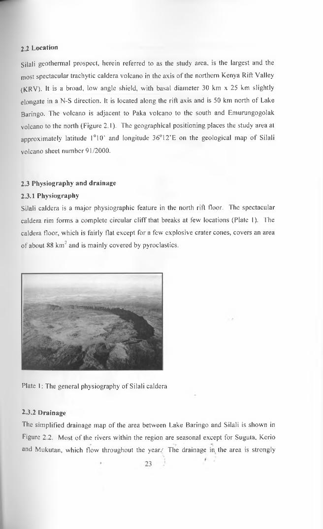
Silali caldera is a major physiographic feature in the north rift floor. The spectacular
caldera rim forms a complete circular cliff that breaks at few locations (Plate 1). The
caldera floor, which is fairly flat except for a few explosive crater cones, covers an area
of about 88 km2 and is mainly covered by pyroclastics.
Plate 1: The general physiography of Silali caldera
2.3.2 Drainage
The simplified drainage map of the area between Lake Baringo and Silali is shown in
Figure 2.2. Most of the rivers within the region are seasonal except for Suguta, Kerio
and Mukutan, which flow throughout the year/ The drainage in the area is strongly

controlled by the structural elements of the region. The crest of the eastern shoulder of
the rift acts as a watershed between rivers that flow westwards through steep gorges
into the inner trough, and the rivers that drain the high plateau and flow eastwards into
EwasoNgiro and eventually into the Indian Ocean.
Figure 2.2: The map of the drainage system in the area between Lake Baringo and Lake Turkana (modified from Dunkley et al., 1993)

The crest of the western shoulder of the rift marked by Baringo Hills to the south and
Loriu Plateau to the north acts as drainage divide between the Kerio system to the west
and drainage into the inner trough to the east. The inner trough consists of two major
drainage systems, namely Lake Baringo and Suguta River to the north of the study area
(Figure 2.2). Several rivers flowing from the south, the southeast and the west feed
Lake Baringo. The main feeder is the Molo River, which rises from the south on the
Mau escarpment but is joined by numerous tributaries flowing off the eastern flanks of
Baringo escarpment. The Endau and Perkerra also drain the Baringo escarpment and
flow into the west side of the lake, whilst the Mukutan and OlArabel drain the Ngelesha
escarpment and flow into the southeastern side of the lake. Suguta River, which is fed
by the seasonal Nginyang River, is the main drainage system north of the project area.
The Suguta is controlled by the northwesterly tilt of the inner trough and the locations
of the axial volcanoes.
2.4 Topography
The major topographical features in the prospect area are river valleys, plains, the hills,
the floor of the Rift Valley and the northern plateau. There are several volcanoes
especially in the the vicinity of the study area and these are Tiati, Paka, Karnugo and
Korosi.
2.5 Climate
The prospect experiences two seasons of rainfall; the long and the short rains. The long
rains start from the end of March to the beginning of June, and the short rains from the
end of September to November. The average rainfall varies from 486 to 755 mm per
year. The mean annual maximum temperature is about 30°C and occasionally rises to
over 35°C. The hottest months are from January to March.
2.6 Vegetation
Three vegetation types namely; evergreen bush, deciduous shrub land and chrysopon
grassland are dominant in the study area. During dry season, the area is mostly bare
ground. Other vegetation noted in the area is the geothermal grass (fibrilytis exillis)
which is found in hot grounds and around the fumaroles.
25/

2.7 Land use and land resources
The study area is 100% Arid and Semi-Arid Lands (ASAL). The local community
(Pokots and Turkanas) in the study area are mainly pastoralist; however, a few have
settled down to farming. Some crop farming is being done in agro-pastoralist livelihood
zones found in Churo, Tangulbei and Koloa division.
2.8 Geology of the study area
Silali is a large Quaternary caldera volcano in the axis of the northern Kenya rift at the
border between Turkana and Pokot East Districts at 1°10’N, 36°12’E (Figure 1.1). The
volcanic shield covers an area of about 850 knr and rises to 760 m above the rift floor.
The summit of the volcano is at 1528 masl and is occupied by a caldera that measures
7.5 km by 5 km and is bounded by 300 m cliffs.
The development of the 30 km wide Silali trachyte shield volcano was initiated during
the early Quaternary times with the eruption of largely basaltic lavas. Subsequent
activity comprised both basaltic and trachytic volcanism, which resulted in the
formation of a low shield volcano.The eruptions composed predominantly of basalts,
trachytes, hawaiite, mugearite, benmoreite and phonolite (Dunkley et al., 1993).
Activity continued and culminated in the incremental collapse of the caldera at the
summit with NW alignment. The simplified geological map of the area is shown in
Figure 2.3.
Basalt and trachyte (Katenmening lavas) erupted along the circumferential fissure zone
and from a major meridional summit fissure forming a series of flat summit benches
and ponded in summit depressions before overflowing. The continuing inward collapse
of the summit area and the lateral drainage of magma from a high level reservoir finally
culminated in the formation of a large caldera at around 63 ka. During the Katenmening
activity, three large pit craters formed on the southern flanks of Silali, probably as a
result of phreatomagmatic activity. The largest Katemening crater is mantled by a
basaltic agglutinate containing many thousands of dorerite blocks (McCall and
Hornung, 1970). Post caldera activity utilized pre-existing weaknesses within the
caldera, erupting basalt and trachyte lavas until around 7 ka within the caldera, and was
contemporaneous with the eruption of trachyte lava domes (9-7 ka).
26 i

(UI) flu (WO
N180000 18S000 190000 195000 200000 205000
Easting (m )
Legend— Alluvium
Rock typesMio-Pliocene lavas and pyroclastic rocks H Summit Trachytes
♦ Pyroclastic cone ] ] Recent basalts Arzett Tuffs
--------Faultline J Black Hills Trachyte lavas and intra-caldera lavas Kapedo Tuffs
j Upper pyroclastic deposits ^ Alluvium
| Katenmening basalts and trachytes | Discoid Trachytes
| Flank Fissure basalts | Lower Trachytes
Figure 2.3: Simplified geological and structural map of Silali volcano. Modified from Williams et al., (1984).
BlackHills trachytes on the eastern flanks and some late tongues of basalt on the outer
slopes are the latest eruptions in Silali and are not dated but are probably about 200 yrs
27

BP judging from the pristine nature of the lavas. Table 1 below shows the stratigraphic
sequences and the evolution of the Silali volcano.
Table 1: Stratigraphy and evolution of the Silali volcano. Modified from Smith et
al., (1995).
Event/eruption Age Activity
Young Basalt lavas 4±2-10±2 ka
WESTERN FLANK ACTIVITY
Summit Trachyte
Arzett Tuffs and Lavas
Discoid Trachyte
Kapedo Tuff
Black Hill Trachyte lavas
Late Pyroclastic Deposit
Upper basalt and trachyte lavas 7±3 ka
CALDERA FORMATION
Katenmening Lavas 64±2 ka
FAULTING AND SUB1SDENCE
Flank Fissure basalt
Upper Pyroclastic Deposit 133±3 ka
FAULTING
Intermediate Lavas
Lower Pyroclastic Deposit
Lower Trachyte Lavas
Mission Basalt
224±9 ka
2.8.1 Structural setting of Silali
The main structures in the area surrounding Silali include the NNE-SSW trending faults
and the caldera. The axial rift zone which has played an important part in the younger
phases of volcanism in Silali shows a change in orientation across the volcano. In the
north, it is parallel to the rift margin and trends NNE-SSW at 018°, whereas in the south
individual deformation belts become narrower, trend more N-S and are oblique to the
rift margins. The faults and fractures in the rift are curvilinear with strike lenghts of
28/

upto 5 km, and are often composed of a series of en echelon segments linked by short
up-faulted horsts or obliquely trending relay or transfer faults.
Figure 2.4: Tectonics of the Silali region with thin lines signifying the numerous faults while the bold dark lines are fissures (Modified from Smith et ah, 1995).
29

Downthrow directions are distributed equally between east and west and displacements
vary from 10-20 metres. Changes in diaplacement directions along individual faults are
not uncommon, particularly on the northern flanks. Post caldera within this zone is also
indicated by numerous faults which cut the caldera walls and the lavas on the caldera
floor. Figure 2.4 below shows the structural setup of Silali.
2.8.2 Geothermal manifestations
The major geothermal manifestations occur within the caldera floor and on the eastern
highly faulted slopes of the volcano and covers an area of about 20 km2. Some
manifestations also occur along river Suguta in the west and along fractures in the far
north of the volcano (Figure 2.5). Manifestations occur in form of altered grounds,
steaming grounds, hot springs and fumaroles. The hottest and most extensive activities
occur in the eastern half of the caldera floor. Temperatures of up to 97°C have been
measured (Geothermal Development Company, 2010). The Kapedo hot springs at the
base of the western slopes of the volcano are the source of Suguta river and they
discharge at 45-55°C with a combined estimated flow rate of about 1,000 1/s. Gas
geothermometry gave temperatures of 238-287°C using hydrogen (GDC, 2010).
In Kapedo, fault zones directly below the discoid trachyte result in a series of hot
springs at the riverbed. Hot springs sprout from faults and fissures in the discoid
trachytes, Kapedo tuffs, lower trachytes and underlying Mission basalts. These hot
springs at the base of the western slopes of the volcano are the source of Suguta River
and they discharge at temperatures of 45-55°C with a combined estimat6d flow rate of
about 1,000 1/s.
In Lorusio Main manifestations include hot springs with measured temperatures
between 65-74°C occurring on a flat pan. The hot springs flow eastwards away from
ranges of hills hosting dyke swarms and volcanic cones. There are about 5 springs
occurring within a discharge area of about 1 km2 of highly altered rock. They are
probably due to upwelling of meteoric waters along a fissure/fault zone after contact
with deep hot rocks.
/
I f30

Figure 2.5 Map showing the geothermal manifestations in the Silali geothermal prospect
/
31t

2.8.3 Hydrogeology
Dunkley et al., 1993 obtained data from records for a total of 70 boreholes, situated
within the floor of the rift and on its bounding intefluves between Lake Baringo and
Lake Turkana. This data has been used to gain information on aquifer properties and
regional groundwater flow patterns. It is important to stress that the borehole data set is
very limited for such an expansive area. It should also be emphasized that aquifer
properties determined by the analyses of borehole records can only apply to depths
penetrated by the boreholes.
2.8.4 The potentiometric map and regional flow patterns
The potentiometric map shown in Figure 2.6 was constructed using borehole water rest
level, borehole data and spring data. Where data was scarse contours have been
estimated by assuming that the potentiometric surface is a subdued replica of the
groundwater surface. The depth to the water table beneath the rift floor from the data
varies from less than 50 m near Korosi to 100 m near Silali. In broad terms,
groundwater flow lines are expected to be perpendicular to the groundwater contours
shown in Figure 2.4, with recharge occuring at high altitude and discharge at low
altitudes. The figure therefore indicates areas of groundwater recharge on the east and
west margins of the rift and a zone of discharge along the rift floor. Flows along the rift
floor are directed northwards from Lake Baringo as far as Lake Logipi which is a
regional discharge area with a water surface level of approximately 270 m above mean
sea level. Lake Turkana lies at an altitude of about 365 m and therefore subsurface
drainage from the lake is directed southwards towards Lake Logipi, passing beneath the
Barrier Volcanic Complex.
The potentiometric data indicates that the regions around the volcanic centres of Korosi,
Paka, Silali and Emuruangogolak are likely to be subjected to groundwater flows both
laterally from the rift margins and axially from the south. The rift margin component
appears to be dominantly from east for Paka, Silali and Emuruangogolak areas and
perharps also for Korosi. Lake Baringo water is likely to be the dominant component of
axial flow within the rift floor in the south of the area, but decreases northwards. The
potentiometric map (Figure 2.4) indicates that the axial flow is mainly directed along
the western side of the inner trough as far north as Emuruangogolak.

The Namarunu area appears to be one of the easterly groundwater flow, with a
component of axial flow, although it is unlikely that Lake Baringo water persists in a
readily identifiable form in this area. In the north of the area, around the Barrier
Volcanic Complex, groundwaters are likely to be dominated by southerly subsurface
flow from Lake Turkana with a strong component of easterly flow from the eastern
margin of the rift around Ngiro.
The hydrogeological model for the system can be explained in terms of upflow and
outflow within the caldera. The recharge is from the rains and mainly from the East, the
fluid then outflows mainly to the west and to the north through formation contacts and
faults and fractures discharging on the surface at the Kapedo springs. The recharge of
the system is mainly from the east which is intensely faulted and to some extent from
the south axially from Lake Baringo and the west.
33

120_ l_
100 200—1—
Figure 2.6: The potentionietric map between Lake Baringo and Lake Turkana (after Dunkley et al., 1993)
120

CHAPTER THREE
3.0 BASIC PRINCIPLES OF THE METHODS USED
3.1 General introduction
In this chapter, the principles of the geophysical methods used to achieve the objectives
of the study are outlined. These geophysical methods used include the Central Loop
Transient Electromagnetics and the Magnetotelluric methods.
3.2 Basic theory for Transient Electromagnetics (TEM) Method
In the central loop TEM method, a constant current is transmitted in a square loop of
wire placed on the ground generating a static primary magnetic field around it. The
current is then turned off abruptly and the decaying magnetic field induces currents in
the ground. These currents decrease, due to Ohmic losses, and the secondary magnetic
field decays with time. Figure 3.1 shows a schematic field layout and Figure 3.2 the
current waveform and the induced voltage in the receiver coil. Just after the transmitter
is switched off, the secondary magnetic field from the current in the ground will be
equivalent to the primary magnetic field (which is no longer there) but, with time, it
will diffuse downwards and outwards resulting in increasing depth of penetration with
time (Figure 3.1).
The magnitude and rate of decay of the secondary magnetic field is monitored by
measuring the voltage induced in a receiver coil usually placed at the centre of the
transmitter loop, as a function of time after the transmitter current is turned off. The
current distribution and the decay rate of the secondary magnetic field depend on the
resistivity structure of the earth with the decay being more gradual over a more
conductive earth (Amason, 1989).
The depth of penetration in the central loop TEM-sounding is dependent on how long
the induction in the receiver coil can be traced before it is drowned in noise. At the so
called late times (described later), the induced voltage in the receiving coil on a
homogeneous half space of conductivity, o, is (Arnason, 1989)
V(t, r) a Io (C( Ho a r 2 )3/2 / / 0nm t5/2), _ (3.1)
where, ( ,35
i

C = A m ir is Ho/2nr\
nr = Number of turns on the receiver coil,
Ar= Area of the receiver coil [m2],
As = Area of the transmitting loop [m2],
ns = Number of turns in transmitter loop,
t = Time elapsed after the current in the transmitter is turned off [s],
Ho = Magnetic permeability [Henry/m],
V(t,r) = Transient voltage [V],
r = Radius of the transmitter loop [m],
Io = Current in the transmitting loop [A].
This shows that the transient voltage for late times after current in the transmitter is
abruptly turned off, is proportional to o 12 and falls off with time as t 5 2. This leads to
the definition of the late time apparent resistivity by solving for the resistivity in
equation 3.1 leading to the equation
pa = p0/4n( UoPoArnrAsns/St5'2 V(t,r) ) 2/3. (3.2)
Depth of probing increases with time after the current is turned off.
Apparent resistivity, pa, is a function of several variables:
• Measured voltage,
• time elapsed from turn off,
• area of loops/coils,
• number of windings in loops/coils,/
• magnetic permeability.
For half-space, apparent resistivity, pa. (and the true resistivity for homogenous earth) is
expressed, in terms of induced voltage at late times after the source current is turned
off, as
Pa(0 = Po 2//0IArAsAn 5t5/2V(t)
2/3
where,
pa =Apparent resistivity,
Ho = Magnetic permeability [Henry/m],
Ar= Area of the receiver coil [m“],
. 36 t

i4i = Area of the transmitting loop [nr],
V(t,) = Transient voltage [V],
t = Time elapsed after the current in the transmitter is turned off.
Figure 3.1: The central loop TEM configuration (from Hersir and Bjornsson, 1991)
37t

Figure 3.2: Basic principles of the TEM method (a) Shows the current in the transmitter loop, (b) Is the induced electromotive force in the ground, and (c) is the secondary magnetic field measured in the receiver coil (from Christensen et al., 2006).
The time behavior of the diffusing current is divided into three phases according to their
characteristics as illustrated on Figure 3.3 which shows the induced voltage as a
function of time for a homogeneous earth. In the early phase, the induced voltage is
constant in time. In the intermediate phase, the voltage starts to decrease with time and
with steadily increasing negative slope on log-log scale until the late time phase is
reached where the voltage response decreases with time in such a way that the
logarithm of the induced voltage decreases linearly as a function of the logarithm of
time. The slope of the response curve in the late phase is -5/2 in accordance with
equation 3.1 which is only valid for the late-time phase.
* f38

Figure 3.3: Voltage response for homogenous half space of 1, 10, and 100 flm (from Arnason, 1989)
The apparent resistivity at early time increases with decreasing resistivity of the half
space and also that the transitions from early to late time get shifted towards earlier
times as the resistivity of the half space increases (Figure 3.4). However, it should be
noted that the response curve has the same shape for the different half space
resistivities. When the apparent resistivity for a homogenous half-space is plotted as a
function of time, it approaches asymptotically the true resistivity of the half-space for
late times.
39

Figure 3.4: Late time apparent resistivity for homogenous half space of 1, 10 and 100 ilm (from Arnason, 1989)
3.4 Basic theory of magnetotelluric methodThe magnetotellurics method is a natural-source, electromagnetic geophysical method
of imaging structures below the earth's surface, where natural variations in the earth's
magnetic field induce electric currents (or telluric currents) under the Earth's surface.
Both magnetic (Hx,Hy and Hz) and electric (Ex and Ey) fields are measured in
orthogonal directions giving two impedance tensors and their phase which are used to
derive the resistivity structure of the subsurface (Figure. 3.5).
40.'

360°
Figure 3.5: MT-soundings Layout
The ratio of the electric field to magnetic field can give simple information about the
subsurface conductivity. The high frequency gives information about the shallow
subsurface with the low frequency providing information about the deeper earth.
The magnetic and electric fields are measured in the frequency range 101 Hz to 10"4 Hz.
This time varying magnetic field comes from two sources with high frequencies (>1
Hz) coming from lightening discharges in the equatorial belt while the low frequencies
(<1 Hz) comes from the interaction between the solar wind and the earth's
magnetosphere and ionosphere. These natural phenomena create strong MT source
signals over the entire frequency spectrum.
The MT method can explore down to hundreds of kilometres, which makes it the EM
method which has the most exploration depth of all the EM methods, and is practically

the only method for studying resistivity deeper than few kilometres.
EM fields is described by the following set of relations, called the
which hold true for all frequencies.
VxE=~n(dH/dt) Faraday’s law,
VxH=J+£(dE/3t) Amperes law,
where,
E: Electrical field intensity (V/m),
H: Magnetic field intensity (A/m),
J: Electrical current density; J = o E (A/mm"),
a: Conductivity (Siemens/m); p =1/ a (Dm),
s: Electrical permittivity (F/m),
p: Magnetic permeability (H/m).
3.5 Electromagnetic induction in a homogenous earth
The ratio of electric to magnetic field intensity is a characteristic measure of the
electromagnetic properties often called the characteristic impedance (Equation 4.3 and
4.4)
Zxy= Ex/Hy= icopo/k, (4.3)
Zyx=Ey/Hx=- iconolk, (4.4)
where,
ZXy, Zyx= Characteristic impedance in x and y directions,/
co =Angular frequency (27rf) where f is frequency (Hz),
Po = Magnetic permeability (H/m),
Ex,y= Electric field intensity (V/m) in x, y direction,
H*,y= Magnetic field intensity (Tesla) in x, y direction,
k = V(io>/z (icoe+ a)) stands for the wave propagation constant,
£ = Dielectric permittivity (C/Vm),
a = Conductivity (Siemens/m).
The term coe in wave propagation constant k is much smaller than conductivity a and
can be ignored, therefore, k =V[icoa]. Putting this into equations 4.3 or 4.4 we get:
Zxy= Ex/Hy= icofi/k ~icon/'l[iooa] = Vi V[a>p/r]= V[a>pp] .e'"/4 (4.5)
The propagation of
Maxwell equations
(4.1)
(4.2)
42t

Z y x ~ E y !H x ~ i c j f l / k --------Zxy ( 4 -6)
Figure 3.6: Homogenous half space response of electric and magnetic field describing the 45° phase difference of the E and H fields, their amplitude are not the same.
Where, tt/4 is the phase angle by which Hy lags Ex as explained on Figure 3.6.
If the earth is homogenous and isotropic, then the true resistivity of the earth is related
to the characteristic impedance through the following relation (e.g. Hermance, 1973).
p= \/pco\ Zxy 12= \/pco \Zyx\ 2 (4.7)
For a non-homogeneous earth, an apparent resistivity (pn) can be defined as if the earth
were homogeneous using this same formula.
In practical units, for homogeneous earth the resistivity, p in the above equation can be
written as:
pa = 0.2T | Z |2=0.2T | Ex/By\ 2, (4.8)
and phase angle 0=arg( Z) =7r/4 or 45°,
where E’ is the electrical field in mV/km, E’ = Ex 10 6, B=pH is magnetic field in
Tesla, B=10 l) Tesla, T is period in seconds and p=47rxl0 7,
43 i

For a non-homogeneous earth, the apparent resistivity (pa) and phase (6a) are functions
of frequency and are defined as follows:-
Pa=0.271 Zol2 (4.9a)
9a=arg( Z0 ) 4 45°. (4.9b)
3.6 Skin depth
Skin depth, 8, is the depth where the electromagnetic fields have reduced to e 1 of its
original value at the surface. The propagation is time dependent on the oscillating
electromagnetic fields, that is H. E ~ e'"', and is vertically incident plane wave.
Therefore skin depth is used as a scale length for the time-varying field, or an estimate
of how deep such a wave penetrates into the earth, and is given by:
<5= \/Real(k)= 1 /Real (icopa)= V[2/copa] = 'J[2Tp/(2n*4nx\0 7)]= IOVttW [20/8]
W [7p],or <5-500 V[7>], (4.10)
where <5 is in metres, T is period in seconds and p in
3.7 MT dead band
MT data acquisition is prone to a number of problems, one of them being the dead band
problem. This occurs in the frequency band between 0.1 Hz to 10 Hz in which natural
signals are typically weak. The power spectrum of these fluctuations plummets in the
frequency range 0.5 - 5 Hz minimizing at 1Hz. This problem is attributable to the
inductive source mechanisms, one effective below -1Hz and another above -1Hz
which causes reduction in data quality. Induction magnetic coils used in MT data
acquisition are not sufficiently sensitive in the dead band to detect the natural
background.
However, it is to be noted that the dead band problem, due to the weak and fluctuating
signals with dominant noise in that band, does not get resolved satisfactorily by robust
processing with the site itself so remote reference processing is used to minimize
distortions at this band and improve on signal to noise ratio. This leads to poor inherent
geometric resolution of target structures at depths near the subsurface (Garcia and
Jones, 2002). ' , "
> 44 j
)

CHAPTER FOUR
4.0 DATA AQUISITION AND PROCESSING OF DATA
4.1 Brief Outline
In this chapter, the methods and instruments used during the field surveys and the data
processing procedures are presented.
Section 4.2 gives an outline of the general approach used in project administration right
from inception to completion. This is a procedure to guide the research in planning,
collecting, analyzing and interpreting observed facts.
Section 4.3 discusses the instrumentation used during the field surveys. The main focus
is on the foundation of each instrument used during the resistivity survey.
Section 4.4, discusses methods used to collect the data used to determine variations in
electrical conductivity of the sub-surface both laterally and with depth at the scale of
field mapping.
A procedure for processing all field data so as to achieve the results of the study is also
discussed critically in section 4.5.
4.2 Research Design
This study involved four main stages, namely;
• Review of available data,/
• Fieldwork,
• Data processing and interpretation,
• Reporting.
1.Review of available data: This step involved the collection and review of all relevant
available literature from existing files, reports, libraries, and the databases for a wide
range of information on Silali, such as:
^ Topographical maps, aerial photographs and satellite images,
> Geographical and geological data,
J

r> Reports of previous geophysical studies (magnetic, seismic, gravity and
electrical resistivity) in the area,
> MT and TEM data files,
> Data on the present energy use and the future energy demand.
The findings of this survey were used to plan the fieldwork in a way that:
> duplication of earlier investigations is avoided,
> data are collected in the significant locations,
> the best results are obtained for the least cost.
2. Fieldwork: The fieldwork involved the execution of magnetotellurics and transient
electromagnetic resistivity sounding at a number of points in the study area.
3. Data processing, interpretation and geothermal modelling: This stage involved
the processing of all the data collected both from the archive and from the fieldwork.
Geophysical anomaly maps and ID apparent resistivity pseudo-section models were
made using the software packages Winglink from Phoenix Geophysics. Integration and
overlay analysis of the processed field results were carried out using the GIS software,
ArcGIS 9.3 from ESRI, and software Surfer of Golden Software Inc.
4. Reporting: This stage included the reporting on the entire work (data collection, data
analysis and interpretation) and establishment of recommendations for future
developments.
This approach has been summarized as shown in Figure 4.1.
46 I

METHODOLOGY
I
iData analysis, integration and interpretation
______________ i __________________Conclusions and Recommendations
Figure 4.1: A schematic illustration of the approach used for during research project.
47
J

4.3.1 Magnetotelluric (MT) method
The instrument used was V5 System 2000 (MTU series i.e Satellite-Synchronized Data
Acquisition Units) from Phoenix Geophysics. The MTU is the heart of the V5 System
2000 (Figure 4.2 below). Introduced in the late 1990s, this patented system has now
been used at tens of thousands of survey sites worldwide. Flexibility of station spacing
from kilometres to tens of metres facilitates cost-effective broad reconnaissance or
resolution of fine details in a variety of applications.
4 .3 F i e l d I n s t r u m e n t a t i o n
Figure 4.2: V5 System 2000(MTU series)
The MT techniques are excellent supplements to seismic methods in hydrocarbon
exploration, but can also be used alone if logistics or geology makes the seismic method
impractical. GPS synchronization means that multiple stand-alone units can be
deployed simultaneously in almost any terrain, with no need for interconnecting cables.
A small number of magnetic channels can be combined with many electric channels to
form an economical system of virtually any size.
The deployment of synchronized remote reference stations permits sophisticated noise-
reduction methods during processing. Several channel complements are available—
electric (E) only, magnetic (H) only, or 2E + 3H combined. The units can be purchased
for MT alone (MTU) or for selectable MT/AMT (MTU-A). Acquisition setup files are
stored on the removable industrial-grade Compact Flash card for automatic operation.
Data files are stored on the same card for easy transfer to the processing PC.

4.3.2 Transient Electromagnetic method
The TEM equipment used is manufactured by Zonge Engineering and consists of a
current transmitter, Transmitter Controller (XMT), GDP-32 receiver, a receiver coil
with effective area of 10000 m2, a voltage regulator and a transmitter loop and a 120VA
three phase power generator as shown in figure 4.4 below.
The transmitter can transmit either frequency domain (100% duty cycle) or time domain
(50% duty cycle) waveforms. This transmitter is suitable for surveys ranging from
laboratory-scale (like core samples) to deep mining, geothermal, or petroleum
exploration. Figure 4.3 below shows a Zonge TEM transmitter used during the field
work.
The XMT-32 Transmitter controller (Figure 4.5) produces timing signals for controlling
all of the Zonge Engineering GGT, ZT, and NT transmitters

Figure 4.5: Transmitter Controllers
Provision is made for synchronizing multiple controllers and GDP receivers. Frequency
control can be accomplished either manually or by a time sequence program which is
loaded through the RS-232C port. The GDP-32 is Zonge Engineering's multi-channel
receiver for acquisition of controlled- and natural-source geoelectric and EM data
(Figure 4.6).
50

The Geophysical Data Processor receivers perform broadband synchronous time or
frequency domain measurements on both controlled-source (i.e., signals generated by
transmitting current into grounded dipoles or wire loops) and on natural fields.
Performance advantages:
• multifunction capability,
• synchronous timing,
• unique multi-channel acquisition.
Unique capabilities:
• Remote control operation,
• Broadband time-series recording,
• High-speed data transfer.
4.4 Field Data Acquisition and Processing
4.4.1 Magnetotelluric (MT) field survey
A total of 134 MT soundings are considered for interpretation in the Silali prospect
covering an area of about 81 km2 as shown in Figure 5.6. The data was acquired using
5-channel MT data acquisition system (MTU-5A) from Phoenix Geophyics.
The layout was made such that the electric dipoles were aligned in magnetic North-/
South and East-West, respectively, with corresponding magnetic channels in orthogonal
directions and the third channel positioned vertically in the ground as can be seen in
Figure 3.5. Before data acquisition, a start-up file was prepared with parameters like
gains, filters, time for data acquisition and calibrations for both equipment and the coils
and stored on a flash disk in the equipment. The ground contact resistance is generally
measured to gauge the electrode coupling to the ground and both high pass filter and
antialiasing filter used with a corner frequency of 0.005Hz to remove the effect of self
potential from the electric dipoles. The electric field was measured by lead chloride
porous pots and the magnetic sensors were buried about 20 cm below the surface to
minimize the wind effect.
51 i

MT data was acquired in frequency range from 104 Hz to 10'4 Hz for a period of about
20 hrs which ensures that deeper investigation of the subsurface is achieved. In this
survey, long period data was not realised in most of the stations because signals were
drowned in noise at low frequencies. The penetration depth of the electromagnetic wave
depends on the frequency.
4.4.2 TEM field survey
In this study a total of 100 Central Loop TEM soundings were carried out in the Silali
area spread over about 65 km". The stations were scattered within the prospect area
with denser coverage inside the caldera as shown in Figure 5.6 using the TEM
equipment described earlier.
Before data acquisition, both the receiver and the transmitter controller high-precision
crystals were warmed up for a period of about an hour and then synchronized to ensure
that induced voltage is measured by the receiver at the correct time after the current turn
off. In the field setup, a 300m x 300m transmitter wire loop was used and a 9 ampere
half-duty square wave current was transmitted at frequencies 16 Hz and 4 Hz. The
transient signal was recorded in the time interval of 36.14psec to 96.85msec at
logarithmically spaced sampling gates after the current turn-off. For each frequency
several repeated transients were stacked and stored in a memory cache inside the Zonge
data logger and later transferred to a personal computer for processing.
4.4.3 Data processing
4.4.3.1 General introduction
For magnetotelluric data a Fourier transform was applied to the time series data
collected and then processed into cross-power estimates. Processing was done and the
cross-powers were then analyzed to obtain an estimate of impedance, resistivity and
phase which was later converted to Electronic Data Interchange (EDI) format using the
Phoenix SSMT processing software. The raw Transient Electromagnetic (TEM) data
were converted to average (AVG) files appropriate for importing into the Winglink
software database for interpretation.
52

The EDI files were then imported to WinGlink software for interpretation. Here
Magnetotelluric data (MT) data were decomposed to principle axes to minimize the
diagonal elements of the impedance tensor.
For the Transient Electromagnetic data, raw data fdes were read and downloaded from
the GDP-32 receiver by using TEM SHRED (a Zonge Geophysics program) and the
TEM-AVG (also a Zonge Geophysics program) was used to calculate averages and
standard deviations of repeated transient voltage measurements and late time apparent
resistivity as a function of time. WingLink (Geosystem) interpretation program was
used to perform one dimensional inversion (ID) on the data. TEM data were then
included to correct for static shifts in MT data. A one dimensional inversion was
initially run for MT and TEM data and later, a one-dimensional (ID) joint inversion of
MT and TEM was run, and finally a two-dimensional (2D) MT inversion.
4.4.3.2 Magnetotelluric static shift correction using Transient Electromagnetic
One of the common problems in interpreting MT data is static-shift. Static-shift is
caused by the presence of small-scale heterogeneities near the ground surface at
stations. The shift is basically a constant vertical displacement of the MT apparent
resistivity curves on a log scale at all frequencies. These shifts are common to almost all
electrical methods where electrode-ground contact is allowed. MT data interpretation
can be very misleading if these shifts are not addressed (Meju, 1996).
Resistivity methods that do not use electrodes, like the transient electromagnetic
(TEM), are less affected by these localized resistivity contrasts (Pellerin and Hohmann,
1990; Cumming and Mackie, 2010). However, on the other hand, the TEM method is
limited by its shallow depth of investigation (usually less than 1km) and can sometimes
be affected by near surface heterogeneities at the initial times of recording. This is
because at initial times, the response corresponds to the very local geology near the
wire loop (Pellerin and Hohmann, 1990). In this study, TEM data were used to correct
for static shifts on MT data that result from near surface conductivity heterogeneity.
The other possible cause of distortion on MT data is topographic changes (Cumming
and Mackie, 2010). However, this effect can easily be handled by including topographic
information during the inversion process. Thus, TEM data were used entirely to correct
for galvanic distortion on MT data. t
53 ) i

Appendix I show some examples of the static shift corrections made to MT data using
TEM data. The static shifts varied across stations in this region. In this figure, the plots
labeled as (i) are the uncorrected apparent resistivity plots while the ones labeled as (ii)
are the static shift corrected resistivity data. It can be observed that only the apparent
resistivity curves incur this shift while the phases of the MT and TEM correlate.
The plots of the apparent resistivity and phases with time show that, the apparent
resistivity determined from the electric field in the north direction (Ex) and the
magnetic field in the east direction (Hy) that is XY, and the other curve which plots the
data for the other two orthogonal horizontal fields, Ey and Hx that is YX values
overlap, but at lower frequencies (longer periods) the values are different (split curves)
with the exception of station silMT24 whose values appear relatively the same at all
frequencies (Appendix 1). This shows that, the dimensionality can be detected from the
apparent resistivity plots. For 1D subsurface (resistivity only varies with depth) the XY
and YX apparent resistivity plots will be similar to the station silMT24. The curves
display a similar trend. However, for a 2D or 3D subsurface (resistivity varies both
horizontally and vertically) the XY and YX data separate, as displayed on stations
silMT55, silMT180, and silMT75. A careful analysis of the onset of these separations
provides the depth at which the subsurface deviates from a 1D structure. At geothermal
systems this information can help to determine the depth extent of the clay cap
(Onacha, 2006).
54 f

CHAPTER FIVE
5.0 DATA ANALYSIS AND DISCUSSION OF RESULTS
5.1 Introduction
In this chapter data obtained from methods deployed in chapter 4 are analyzed and
results are discussed. The chapter is divided into four sections 5.1, 5.2, 5.3 and 5.4.
Section 5.1 introduces the general approach used during data analysis and discussion of
results. This is a procedure to guide the research in analyzing and interpreting observed
facts so as to achieve the objectives of the study.
Section 5.2 gives an outline used in one dimension (ID) inversion and
interpretation.Further, results in form of iso-resistivity maps at varying elevations are
also presented.
Section 5.3, discusses the two dimension (2D) resistivity inversion results showing
significant variations in the resistivity distribution both vertically and horizontally on all
profiles.
Section 5.4, discusses the essential features considered while the conceptualized
geothermal model was being modelled.
5.2 One dimension (ID) inversion and interpretation
For 1D inversion, it is assumed that the resistivity only varies in the vertical direction
and is laterally constant. In this study, rotational invariant determinant JVIT data were
used for the ID Occam (minimum structure) inversions (Constable et al., 1987) (Figure
5.1). These data have the capability to reproduce 3D resistivity structures (Arnason et
al., 2010; Cumming et al., 2000). 1D Occam inversions were run for MT and TEM data
separately using the WinGlink software. Then the TEM plots were incorporated into the
MT for static shift correction as shown in Appendix 1.
Studies have shown that 1D joint inversion/interpretation of MT and TEM data not only
solves the static shift problem but also enhances the resolution of the subsurface
resistivity when inverted together for geological structures (Cumming and Mackie,
2010; Arnason et al., 2010). The integrated approach involves two related data
(resistivity) sets to optimize a model with better constraints on the inversion. In this
way, the problem of layer suppression is reduced while mitigating the highs and lows in55 ) ' •’

the resistivity equivalences that may be encountered without incorporating the TEM
data. Examples of typical 1D Occam inversion models of MT data after correcting for
static shift are shown in Figure 5.1.
The resistivity models show a resistive top layer overlying a conductive (less resistive)
layer at about 500 m depth. The base of the conductive layer is at about 1000 m depth.
The resistive layer overlies a less resistive layer at a depth below 2000 m. In general,
most of the MT soundings in this region have a similar trend where a conductor exists
at 1000 m depth. This is interpreted as hydrothermal alteration product (clay cap)
(Wright et al., 1985). This lateral conductor overlies a resistive zone that is interpreted
as a region of higher temperature altered rocks (Onacha 2006; Spichak and Manzella,
2009; Ingham, 2004).

Mode INVARIANT1D Model
Resistivity (ohro-m)
Sounding silmt172
Area Silali
Mode INVARIANT1D Model
Resistivity (ohm-m)
Sounding silmt23
Area: Silali
Figure 5.1: One-dimensional Occam resistivity inversion models of MT data at station silMT172 and silMT23.
Maps of resistivity versus elevation were generated from the ID Occam inversion result
(Figures 5.2-5.5). These maps show the lateral resistivity distribution around the Silali
region at a particular elevation. These figures $how resistivity at depths of 500, 1000
* 57 ) ' •’
(

meters above sea level and 2000 and 5000 m below sea level. At shallow depths (500 m
above sea level), the Silali region is in general conductive (low resistivity) (Figure 5.2).
A north-south striking resistivity gradient almost dissects the Silali calderas in two to
form an eastern conductive (less resistive) and a western less conductive (resistive)
section.
(a) Resistivity at 500 masl
At 500 masl (Figure 5.2), three distinct low resistivity (< 6 Qm) areas are clearly seen;
one large region to the east of the caldera towards Black Hills, one to the north-east of
the caldera and another on the south-eastern parts of the caldera near Kuttung area.
These low resistivity zones could probably be as a result of low temperature
hydrothermal clay minerals like smectite and zeolite. On the other hand, the south
western side of the caldera around Katenmening area is characterized by high
resistivities which are probably as a result of un-altered rocks near the surface.
180000 190000 200000
180000 190000 200000
Eastings (m)
Figure 5.2: Resistivity at 500 m above sea level
58 )
r

(b) Resistivity at sea level
At sea-level (Figure 5.3), the general resistivity structure of the prospect indicate a high
resistivity (about 49 ohm-m) particularly within the caldera and in the south western s
ide in the Katenmening area. This high resistivity portion could probably be associated
with high temperature alteration minerals such as chlorites and epidotes. Some higher
resistivity zones can be seen appearing on the southern part of the prospect area and
another in the north-western side of the caldera aligning in the NE-SW direction.
Slighty low resistivity values are still seen on the eastern part around Black Hills area.
140000
ohm.m
130000
120000
9563534235282317151211987654
130000
120000
140000 1-
180000 190000 200000
180000 190000 , 200000Eastings ( m)
Figure 5.3: Resistivity at sea level
(c) Resistivity at 2000 mbsl and 5000 mbsl
Figures 5.4 and 5.5 shows resistivity at 2000 mbsl and 5000 mbsl. respectively. These
figures reveal low resistivity bodies at depth that could be related to magmatic heat
sources. Three distinct low resistivity anomalies can be seen in the prospect area, one in
the eastern part of the caldera towards the Black Hills , the other in the north eastern
part of the caldera and the third towards Kuttung area.
r

Nor
thin
gs (m
)180000 190000 200000
140000
180000 190000 200000
Eastings (m)
Figure 5.4: Resistivity at 2000 m below sea level
9563534235282317151211987654321
60 t

180000 190000 200000
180000 190000 200000Eastings (ml
Figure 5.5: Resistivity at 5000 m below sea level
A low resistivity anomaly spreads almost in the entire survey area with more
prominence in the eastern part of the prospect area from the centre of the caldera
(Figure 5.5). This probably is a heat source extending towards the eastern part of the
prospect area. The relatively high resistivity seen in the upper elevation is still present
which shows that the heat source is structurally controlled./
5.3 Two dimension (2D) inversion and interpretation
In 2D inversion process, it is assumed that the resistivity varies vertically (z) and in one
lateral (either x or y) direction while in the other lateral direction (either y or x), the
resistivity is constant. It is also assumed that the soundings along a profile are
perpendicular to the geo-electric strike. During data collection, the MT instrument
layout has the E lines and H coils oriented in the north-south and east-west directions,
respectively, which does not necessarily coincide with the geo-electric strike (Figure
3.4). The data is rotated so that one axis is perpendicular and the other parallel to the
geo-electric strike before running the inversions. Hence the data is polarized in two
modes. The Transverse Electric (TE) mode is achieved when the electric field is parallel61 ; '

to the geo-electric strike while the Transverse Magnetic (TM) mode requires that the
electric field be perpendicular to the geo-electric strike. The inversion results shown
here include both the TE and TM modes (assumed to be an average of the two modes).
In this section, we aim to obtain 2D images and show the resistivity distribution from
the surface to 7000 m below sea level. To achieve this objective, we applied a 2D
smooth inversion for both transverse electric (TE) and transverse magnetic (TM) modes
on MT data along several profiles as shown in the figures below. In all the inversion
results, the root mean square (RMS) errors were less than 5. The number of iterations
was set to 45. This number was picked after running several inversions with iterations
ranging from 30 to 60. We realized that 45 iterations were good since additional
iterations beyond this value either did not change or had very little effect on the final
result. Figure 5.6 below shows lines over which 2D inversions were run.
uoooo
130000
120000
180000 190000 200000
180000 190000 200000Eastings (mj
Figure 5.6: Silali contour map showing the sounding points
In general, the 2D resistivity inversion results show significant variations in the
resistivity distribution'both vertically and horizontally on all profiles. A lateral\ ' '
62 } ' ;
r
conductor at about sea level shows up on all profiles. The conductor displays a varied
thickness at all profiles. In high temperature geothermal systems, a shallow (about 1000
m depth) lateral conductor is after a hydrothermal alteration product (clay) (Cumming
and Mackie, 2010; Spichak and Manzella, 2009; Ingham, 2004). The lateral conductor
overlies a resistive zone in almost all the two-dimensional resistivity models (Figures
5.7-5.12). In several profiles (i.e., Figures 5.7, 5.8, 5.9), the resistive zones have
signatures of nearly vertical conductors. The nearly vertical conductors are interpreted
as fluid filled fracture systems/faults.
We group the 2D resistivity inversion models into four categories: profiles that trend
east-west, profiles that trend north-south, the profiles that trend northwest-southeast,
and profiles that trend northeast-southwest.
5.3.1The east-west oriented profile lines.
a) Three east-west profile lines were drawn as shown in Figure 5.6 and their two
dimensional inversion results shown in Figures 5.7-5.9. The line that cut through the
caldera (Figure 5.6) shows a low resistivity layer that spreads laterally across the
caldera. This low resistivity layer (conductor) shows significant low resistivity (less
than 15 ohm meter) to the immediate west and far right of the caldera. The depth extent
of this lateral conductor varies across the profiles from about 1000 m depth near to the
caldera to over 3000 m away from it as shown in figure 5.7.
63 i
(

W e s t C aldera E a s t
0 2000 4000 8000 8000 10000 12000 14000 16000 18000
Vertical Exaggeration = 1.10 Distance (m ) L in e I
Figure 5.7: Two-dimensional resistivity cross-section along E-W Line 1 cutting through the Silali prospect in the north of the caldera.
Figure 5.8 also shows a nearly vertical conductor located at the central east section of
the caldera. This low resistivity is thin at shallow elevations and the thickness increases
with increasing depth. The resistivity variation trending east of the caldera was also
observed on elevation slices of the resistivity maps (Figure 5.8 and 5.9). The vertical
conductor zone is interpreted as a fault zone with fluid abundance. This interpretation
applies to the north trending profiles (Figure 5.6).
/
64 !

a&
3000
1000
-1000
2000
-3000
-6000
West Caldera E a s t4000
0 2000 4000 6000
Vortical Exaggeration =1.2
8000 10000 12000 14000
Distance (m)16000 16000 2 0000 22000
Line 2
O tim .m
Figure 5.8: Two-dimensional resistivity cross-section along E-W Line 2 cutting through the Silali prospect in the south of the caldera.
West East3000
H a » 0 P 8! ml
•-70002000 4000 6000 8000 10000 12000 14000 16000 18000 20000 22000 24000 26000 28000
Distance (m )
2 4 6
1 0 8
76
7 0
6 5
5 0
4 5
34
26
20
12
8
V e rtic a l E xag g era tio n ■ 1 .8 V Line 3
Figure 5.9: Two-dimensional resistivity cross-section along E-W Line 3 cutting through the Silali prospect in the south of the caldera.
t
65 i

5.3.2 The North-South oriented profile lines.
To investigate the southward extent of the observed high resistivity west of the caldera
and the low resistivity east of the caldera, a profile line was drawn far south of the
caldera (Figure 5.6). Interestingly, the vertical low resistivity zone is suppressed in this
section. There appears to be a connection between the shallow (about 1000 m below sea
level) low resistivity zone and the low resistivity at depths is 6000 m below sea level
Figure 5.9. The top and bottom resistivity connection could suggest a fault; however,
the lack of a significant low as in Figures 5.10 & 5.11 could imply that this fault has
less fluid.
Figure 5.10: Two-dimensional resistivity cross-section along the north-south profde line 4 running west of the caldera.
N o rth Summit4000
3000
2000
1000
0•§• -1000 6g- -2000
-3000
-4000
-5000
-6000
-7000
0 5000
Vertical Exaggeration = 1.150
South4000
10000 15000
Distance (m)20000
Line 4
3000
2000 Ohm.m
1000
0-1000
-2000
-3000
0̂00 -5000
-6000
-7000
246108
76706559
453426
2012

N o r t h Caldera S o u t h4000
fa
4000 -r
3000 -
2000 -
1000 -
o A -1000 A
-2000 A
-3000 A
-4000 J
-5000 A
-6000 -I
-7000 i
r 3000
2000
1000
0-1000
-2000
-3000
-4000
-5000
-eooo-7000
0 5000
Vortical Exaggeration = 0.950
10000
Distance (m)15000
Line 5
Ohm.m
246106767085594534262012a4
Figure 5.11: Two-dimensional resistivity cross-section along the north-south profile line 5 running east of the caldera.
5.3.3 The northwest-southeast oriented profile lines.
The general trend of faults around the Silali area is northeast from Figure 2.4 above.
Hence, to investigate the depth extent of these faults, northwest trending profiles lines
shown (Figure 5.6) were drawn. Figure 5.12 is a profile southwest of the caldera and
does not cut through the caldera while figure 5.13 cuts through the caldera. The base of
the clay cap (low resistivity) is shallow near the caldera (less than 1000 m below sea
level) and extends to deeper levels away from the caldera along this profile. There are
dipping conductors that are almost vertically oriented east of the caldera. These
conductors are interpreted as faults.
67 /

N o r t h w e s t So ut he as t4000
E
Ia-4000
-6000
3000
2000
1000
0-1000
-2000
-3000
-4000
-5000
-6000-7000
0 5000
Vertical Exaggeration - 1 099
10000Distance (m)
15000 20000
L ine 6
O h m .m
246106
76706559453426201284
Figure 5.12: Two-dimensional resistivity models of the northwest-southeast profiles cutting west of the caldera and the Silali summit.
ex:£
N o rth w est Caldera4000
3000
2000
1000
0-1000
-2000
-3000
-4000
-5000
-6000
-7000
Southeast4000
3000
2000
1000
0-1000
-2000
-3000
-4000
-5000
-6000
-7000
0 5000 10000 15000
Vertical Exaggeration ■ 1.35 D is tan ce (m )
20000 25000
L in e 7
Ohm in
240108
76700559453420201284
Figure 5.13: Two-dimensional resistivity models of the northwest-southeast Line7 cutting through the caldera.
68
/
I/

5.3.4 The southwest-northeast oriented profile lines.
The profile line that trends northeast-southwest (Figure 5.6) was not expected to show
much resistivity variations since it was assumed that it cuts along the fault line. This
profile line runs southeast of the Silali caldera but does not cut through the caldera. The
resistivity distribution along this profile shows a lateral conductor (cap rock) above and
a nearly vertical conductor in an otherwise resistive zone below and is interpreted as a
fluid filled fracture system (Figure 5.14).
The low resistivity layer at about 1000 m below sea level spreads throughout the profile
lines. For a typical high temperature geothermal system, this will be clays rich in
smectite and or zeolite (Cumming et al., 2000). The resistive zone that lies immediately
below this conductor represents high temperature clays (Arnason et al., 2010; Spichak
and Manzella, 2009).
f&
Southw est4000 ~|----------------------
3000 -
2000
1000
0-1000
-2000
-3000
-4000
-5000
-6000
-7000
N o rth east4000
3000
2000
1000
0-1000
-2000
-3000
-4000
-5000
-6000
-7000
0 5000
Vertical Exaggeration » 1.6
10000 15000 20000
Distance (m)2S000 30000
Line 8
Ohm.m
246108
76706559453426201284
Figure 5.14: Two-dimensional Resistivity cross-section along NW-SE Line 8.
A proposed resistivity conceptual model for high temperature geothermal system
requires that a conductive hydrothermal alteration zone .(clay cap) overlies a less
conductive (resistive) zone (Pellerin et al., 1996; Cumming et al., 2000). The resistivity
of these zones is related to temperature dependent hydrothermal alteration processes
(Flovenz et al., 2005). At low temperatures (but above 70°C), clay minerals like
smectite and zeolite are the dominant hydrothermal alteration products (Cumming et al.,/ \ \\ *69

2000). High concentration of smectite and zeolite minerals within the rock matrix will
reduce its electrical conductivity. At higher temperatures (up to 180°C), chlorite and
illite minerals form from hydrothermal effect. These minerals do not conduct
electricity. And hence, high amounts of illite and chlorite within the rock matrix will
increase its electrical resistivity. The concentration of illite and chlorite minerals
increases with increasing temperature. At temperatures of about 220°C and 240°C,
smectite and zeolite are never present and the only minerals are illite and chlorite
(Flovenz et al., 2005; Cumming et al., 2000).
The reduced resistivity in the smectite dominated zones is attributed to the electrical
double layer otherwise known as surface conduction (Flovenz et al., 2005). This surface
conduction happens because of the movement of free mobile ions through the system.
The freedom of ions is suppressed in the chlorite and illite rich zones and hence
increases in resistivity (Flovenz et al., 2005). In the high resistivity region, low
resistivity zones can occur and this has often been related to an increased porosity
(fractures) and hence fluids as in the Coso, Krafla, and Olkaria geothermal system in
California, Iceland and Kenya, respectively, (Newman et al., 2008, Onacha, 2006;
Lichoro, 2009). However, the high resistivity in the chlorite- illite mineral dominated
zone does not necessarily imply the absence of hydrothermal fluids. This could happen
when the conductivity due to the hydrothermal fluids is suppressed by the abundance of
the chlorite and illite and sometimes epidote minerals (Cumming et al., 2000; Flovenz
et al., 2005).
In this study, MT data together with TEM data were used to characterize the Silali
volcanic zone for its geothermal potential. Both 1D and 2D inversion models reveals a
picture of a typical high temperature geothermal system around the Silali caldera
(Amason et al., 2010; Cumming et al., 2000; Spichak and Manzella, 2009). The
resistivity data show a low resistivity (conductor) at shallow depth (about 0 -1000 m
below sea level) which sits on top of a high resistivity zone. This conductor could be
related to high temperature hydrothermal alteration product: the clay cap (Cumming
and Mackie, 2010; Cumming et al., 2000; Wright et al., 1985). The conductivity in
these regions is probably enhanced by smectite and/or zeolite minerals.
70

The increase in the resistivity of the underlying layer can be attributed to the transition
from the conductive smectite mineral to resistive illite and chlorite minerals. This high
resistivity zone is generally perceived to be the geothermal reservoir (Pellerin et al.,
1996; Flovenz et al., 2005/ Hence the conductivity of the reservoir is influenced most
by the resistive illite clays than by the fluids confined within the reservoir fractures.
However, in complex geothermal systems where faulting, hydrothermal alteration, fluid
distribution, and fluid salinity affect resistivity, it is difficult to isolate unique
relationships on resistivity signatures. In turn, this will often give room for
unambiguous interpretation to the observed resistivity signatures.
In some cases, a low resistivity may occur in the illite-chlorite dominated zones. Our
data show this type of anomalies as nearly vertical conductors. Similar conductors have
been observed at Coso geothermal field and Olkaria geothermal field and were
interpreted as zones of high fracture porosity and fluid abundance (Lichoro, 2009;
Newman et al., 2008). We place a similar interpretation to the vertical conductor
observed east of the Silali caldera.
From the ground surface to the base of the clay cap, the apparent resistivity plots show
ID characteristic (XY resistivity overlies the YX resistivity) as shown in Figure 4.8.
However, at depth below the base of the clay cap rock, most of the stations show a
separation of the XY and YX resistivity values (Figure 4.8). Onacha (2006) suggests
that the splitting of these data begins at the base of the clay cap rock and the split is an
indicator of the deviations from one dimensionality.
Results from the resistivity cross-sections derived from the 1-D joint MT and TEM
inversions in the study area reveals three layers namely: a very shallow high resistivity
layer of > 100 ftm, an intermediate low resistivity layer of > 10 Dm underlying the
upper high resistivity layer, and a deep high resistivity layer with values greater than 50
ftm underlying the low resistivity layer. MT resistivity cross-section also shows low
resistivity at few kilometres depth below sea level that could be related to heat sources
for this part of the field.
71 i

5.4 Conceptualized Geothermal Model
5.4.1 Silali Hydrothermal System
The apparent indicators for essential features for development of geothermal system(s)
are discussed below.
5.4.2 Heat source
The continued eruption (post, intra caldera) indicates that the magma chamber below
Silali caldera is still active (molten and hot). The Silali trachytes contain both silica-
oversaturated and silica under-saturated varieties. The oversaturated types occur in the
western flanks with the pre-caldera group while the caldera wall and post caldera
groups are under-saturated (Macdonald et al., 1995). In the post caldera group,
increasing differentiation is thought to have resulted in progressive silica under
saturation. The Blackhills trachytes are critically under-saturated with respect to silica.
A general progression from two-feldspar trachytes to the dominant, one-feldspar
varieties is accompanied by a decrease in phenocryst abundances with more evolved
trachytes tending to be aphyric and glassy. The youngest activity on Silali erupted
porphyritic olivine basalt on the north-eastern flanks of the caldera from a series of
small scoria cones. There is lack of vegetation here suggesting that activity may have
taken place only a few years ago probably 200-300 years ago (Dunkley et al., 1993).
5.4.3 Recharge and permeability
Silali prospect is located on the rift floor where hydrogeologic regime comprises of
recharge of meteoric waters from the higher rift scarps mainly from the east, i.e., the
Laikipia ranges and to some extent from the west, i.e., the Tiati hills. The intense rift
floor fracture/faulting resulting from extensional tectonics of regional rifting in this area
i.e., NNE and some EW structures, provide a good structural set up that allows water
from the rift scarps to penetrate deep into the crust towards the magma bodies under the
rift floor and normal faults conducting hot fluids from deep into possible geothermal
reservoirs at shallower depth. The E-W lineament and the NNE fissure swarm may be
such an important conduit of deep fluids, thus important geothermal controlling features
in the area.
72 /

5.4.4 System capping:
Silali Volcano eruption included issue of several extensive blankets of pyroclastics.
The spread of this debris, preferentially to the north and NW, is evidenced by the way
the rift floor faults are masked in the area. Glassy component pyroclastics are
susceptible to alteration forming hydrated clays that are the cause of self-sealing and the
layered pyroclastics formation becoming very good capping for geothermal systems.
5.4.5 Geothermal System
Studies reveal that a high temperature geothermal system exists under Silali caldera
within the prospect. It is envisaged that the reservoir is hosted within fractured trachytes
and associated pyroclastics of Silali formation and flood trachytes of the Kenya rift
floor. The intense fracturing of the formations is likely to have created high
permeability within the reservoir; however, it is expected that some regions could have
effects of sealing by dyke intrusions. It is envisaged that the reservoir primarily exists in
the central part of the caldera but extends to the eastern side.
The main upflow of the geothermal fluids is postulated to be around the centre of the
caldera and extending mainly east and southeast of the caldera. Resistivity data
indicates the eastern half of the caldera to have high potential as evidenced by lower
values. The top of the reservoir is to be expected to be at a depth of between 800-3,500
m and outflows at shallow levels to the east. From the above, a conceptualized
geothermal model of the study area has been developed and is shown in Figure 5.15.
i73

Baringo Ranges
1000-
Losiolo Escarpment
-4000
-5000
-6000
-7000
LEGENDESI Upper Trachyte/Basal and pyroclastics□ a Lower Trachyte/ Basalt3P! Pleistocene lavas and associated PyroclasticsH Plio-Pleistocene lavas and associated pyroclasticsi s Faulted Miocene lavas
Unidentified crystalline rocks [ H Magmatic intrusive
^ Cold recharge
^ Hot up flow
Fault
Scale
Figure 5.15: The E-W conceptualised geothermal model of Silali caldera along A- A” in Figure 2.3
i74

CHAPTER SIX
6.0 CONCLUSIONS AND RECOMMENDATIONS
Based on the results, the resistivity structure of the study area has been divided into 1) a
shallow high resistivity zone (> 100 Dm) to about 300 m below the surface which is as
a result of unaltered rocks, 2) An intermediate low resistivity zone (10 dm ) to depths
of about 1 km which is as a result of low temperature hydrothermal alteration minerals,
3) A deeper high resistivity (> 50 fim), up to 3-4 km depth indicating high temperature
minerals occurring at depth. The shallow boundary between an upper, low resistive
layer and the underlying intermediate resistivity zone at depths of 800-3500 m appears
to mark the change in clay mineralogy from low grade alteration mineralogy
represented by smectite to high grade alteration mineralogy represented by chlorite,
epidote and actinolite, which is interpreted as the geothermal reservoir zone of this
study area, and 4) a deeper low resistivity region, at a depth of about 5000 m below sea
level is inferred to be magmatic material or intrusion i.e., the heat source of this study
area.
The resultant 2-D resistivity models showing significant variations in the resistivity
distribution both vertically and horizontally on all profiles indicate major structural
controls of the geothermal system.
Further, the study area seems to host a much larger geothermal resource under Silali
caldera and extends to the eastern flanks covering an area of about 75 km" than
previously thought. The system appears to cover much larger area than the coverage of
soundings. The resource potential area has been determined using combined TEM and
MT resistivity anomaly at 5,000 m depth. Using a conservative value of an average of
15 MWe per square kilometer, it is estimated that more than 1125 MWe can be
generated from the identified resource at the study area.
It is therefore recommended that, more long period magnetotelluric (MT) and transient
electromagnetic (TEM) data at the same area be acquired in order to define the extent of
this field and 3-D interpretation be carried out to define three-dimensional features both
laterally and vertically. However, to reduce ambiguities _ in resistivity data
interpretations, constraints from other geophysical data (i.e. gravity and seismic),. 75 ) ' ;

geological, geochemical, and heat-flow data can greatly improve these interpretations
before any drilling is done. In addition, exploratory wells should be drilled to about
3,000-m depth in the caldera and on the eastern flanks (Figure 6.1) of the caldera to
confirm the characteristics and potential of the geothermal reservoir.
160000 110000 200000
160000 190000 200000fairings (m)
Figure 6.1: Resistivity anomaly map at 5000 mbsl showing the proposed wells.
/
76

REFERENCES
Achauer, U and the KRISP Teleseismic Working Group, 1994. New ideas based on the
Kenya rift based on the inversion of the combined dataset of the 1985 and
1989/90 seismic tomography experiments. Tectonophysics,. 236, p.305-329.
Achauer, U., 1992. A study of the Kenya rift using delay-time tomographic analysis and
gravity modeling. Tectonophysics, 209: 197-207.
AFREPREN (2004c). The Potential Contribution of Non-Electrical Renewable Energy
Technologies (RET’s) in Poverty Alleviation in Eastern Africa: The Case of
Wind Pumps, Ram Pumps and Treadle Pumps in Kenya and Tanzania, Nairobi,
African Energy Policy Research Network(AFREPREN)
AFREPREN (2005a) AFREPREN Occasional Paper 26. Renewables in Kenya’s
Electricity Industry: A Review of Geothermal and Cogeneration Technologies,
Nairobi, African Energy Policy Research Network (AFREPREN)
AFREPREN/FWD (2006) Influencing policy through the Active Involment of a
Reseach Institution in the Performance Contract Process- Lessons from the
Experience of AFREPREN/FWD, Nairobi, Energy, Environment and
Development Network for Africa (AFREPREN/FWD).
Arnason, K., 1989: Central-loop transient electromagnetic sounding over a horizontally
layered earth. Orkustofnun, Reykjavik, report OS-89032/JHD-06, 129 pp.
Arnason, K., Eysteinsson, H., Hersir, G. P., 2010. Joint ID inversion of TEM and MT
data and 3D inversion of MT data in the Hengill area, SW Iceland.
Geothermics, 39, 13-34.
Arnason, K., Karlsdottir, R., Eysteinsson, H., Flovenz, O.G., and Gudlaugsson, S.Th.,
2000: The resistivity structure of high-temperature geothermal systems in
Iceland. Proceedings of the World Geothermal Congress 2000, Kyushu-Tohoku,
Japan, 923-928.
Balia, P. (2005) National Study on Small Hydropower Development Status and
Potential of Small Hydropower Development in the Tea Industry in Kenya,
unpublished report, Nairobi and Mombasa, UNEP/GEF and East African Tea
Trade Association (EATTA).
\ \\ f
/
77

Balia, P. (2005) The Potential Contribution of Non-Electrical Renewable Energy
Technologies (RETs) towards Poverty Alleviation: Non-Electrical water
pumping technologies for irrigation, Nairobi, Energy, Environment and
Development Network for Africa (AFREPREN/FWD).
Berktold, A. (1983). Electromagnetic studies in geothermal regions. J. Geophys. Surv
6.173-200
Brace, W.F., and Orange A.S. 1968: Further studies of the effects of pressure on
electrical resistivity of rocks, J. Geophys. Res. 73-16, 5407-5420.
Brace, W.F., and Orange A.S. 1968: Further studies of the effects of pressure on
electrical resistivity of rocks, J. Geophys. Res. 73-16, 5407-5420.
Christensen, A., Auken, E., and Sorensen, K., 2006. The transient electromagnetic
method. Groundwater Geophysics, 71, 179-225.
Clarke, M.C.G., Woodhall, D.G., Allen, D., and Darling, G., 1990: Geological,
volcanological and hydogeological controls o f the occurrence o f geothermal
activity in the area surrounding Lake
Constable, S., Parker, P., Constable, C., 1987. Occam's inversion: a practical algorithm
for generating smooth models from electromagnetic sounding data. Geophysics
52. pp. 289- 300.
Cumming, W., Mackie, R., 2010. Resistivity imaging of geothermal resource using ID,
2D, and 3D MT inversion and TDEM static shift correction illustrated by a
Glass mountain case history. Proceeding World Geothermal Congress, 2010.
Cumming, W., Nordquest, G., astra, D., 2000. Geophysical exploration for geothermal
resources: an application for combined MT -TEM. In: Society of exploration
Geophysics Annual Meeting Teaching program expanded Abstracts, 6-11
August, Canary, Canada, pp. 1071-1074.
Dakhnov, V.N., 1962: Geophysical well logging. Q. Colorado Sch. Mines, 57-2, 445
pp.
Dunkley, P.N., Smith, M., Allen, D.J. and Darling, W.G. 1993. The geothermal activity
and geology of the northern sector of the Kenya Rift Valley. British Geol. Surv.,
Research Report. Ministry of Energy, Kenya.
Fairhead, J. D. and Stuart, G. W., 1982. The seismicity of the East African rift system
and comparison with other continental rift, In G. Palmason (editor),
Geodynamic series AGU, Washington DC, 8:41 -61.• \ t
78

Fairhead, J. D., 1976. The structure of the lithosphere beneath the Eastern rift, East
Africa, deduced from gravity studies. Tectonophysics, 30: 269-298.
Flovenz, O., Spangenberg, E., Kulenkampff, J., Anarson, K., Karlsdottir, R., and
Huenge, E. 2005. The role of electrical conduction in geothermal exploration.
Paper presented at the World Geothermal Congress, Antalya, Turkey.
Garcia, X., and Jones, A.G., 2002: Atmospheric sources for audio-magnetotelluric
(AMT) sounding. Geophysics, 67, 448^158.
GOK (2002b) National Development Plan 2002-2008, Nairobi, Government of Kenya
(GOK).
Hamilton R. M., Smith B. E., and Knopp F., 1973. Earthquakes in Geothermal Areas
near Lakes Naivasha and Hannington (Bogoria), Kenya. Unpublished report to
the UNDP/EAP&L.
Hamilton R.M. and Muffler, L. J. P. 1972. Micro-earthquakes at the Geysers
Geothermal area, California. J. Geophys. Res.,77, no. 11, 2081-2086
Henry, W.J., 1987. A seismic investigation of the Kenya Rift Valley. PhD thesis,
University of Leicester, Leicester. 214pp
Henry, W.J., Mechie, J., Maguire, P.K.H., Khan, M.A., Prodehl, C., Keller, G.R., and
Patel, J., 1990. A seismic investigation of the Kenya rift valley. Geophys. J. Int.
vol. 100, pp. 107-130.
Hermance, J.F., 1973: Processing of magnetotelluric data. Physics o f the Earth and
Planetary Interiors, 7, 349-364.
Hersir, G.P., and Bjornsson, A., 1991: Geophysical exploration for geothermal
resources. Principles and applications. UNU-GTP, Iceland, report 15, 94 pp.
Ingham, M. 2004. High resolution electrical imaging of fault zones. Phy. of the earth
and planetary interior. 150. p. 93-105
Kearey, P., and Brooks, M., 1994: An introduction to geophysical exploration (2nd
edition). Blackwell Scientific Publ., London, 236 pp.
Keller, G. R., Mechie, J., Braile, L. W., Mooney, W. D. and Prodehl, C., 1994. Seismic
structure of the uppermost mantle beneath the Kenya rift. In C. Prodehl, G. R.
Keller and M.A Khan (Editors), Crustal and Upper Mantle structure of the
Kenya Rift. Tectonophysics, 236: 201-210.
79 I

Keller, G.R., Prodehl, C., Khan M.A., Morgan, P., Braile, C.W., Ulsen, K.H.,
Wendlandt, R.F., and Baldridge W.S., 1994. The East African Rift system in
the light of KRISP 90. Tectonophysics, 236: 465-483.
Keller, G.V., and Frischknecht, F.C., 1966: Electrical methods in geophysical
prospecting. Pergamon Press Ltd., Oxford, 527 pp.
KNBS (2006) Kenya Facts and Figures, Kenya National Bureau of Statistics (KNBS)
KPLC (2006). Annual Report, 2006, Nairobi Kenya Power and Lightning Company
(KPLC)
Lee Lemer, K., Lerner, B.W., and Cengage, G., 2003: Porosity and permeability.
World of Earth Science, Retrieved from http://www.enotes.com/earth-science/
Lichoro, 2009., Joint 1-D inversion of TEM and MT data from Olkaria domes
geothermal area, Kenya. Paper presented at the UNU geothermal Training
Programme.
Mariita, N. O., Keller, G. R., 2007. An integrated geophysical study of the northern
Kenya rift. J. Afr Earth Sc. 48, 80-94.
Mariita, N.O. 2003. An integrated geophysical study of the northern Kenya rift crustal
structure: implications for geothermal energy prospecting for Menengai area. A
PhD dissertation, University o f Texas at El Paso, USA.
Meju, M. A., 1996. Joint inversion of TEM and MT data soundings: some effective
practical considerations. Geophysics, 61. 56-65.
MOE, 2002. Study on Kenya's Energy Demand, Supply And Policy Strategy for
Households, Small Scale Industries and Service Establishments, Ministry of
Energy (MOE)
Newman, G. A., Hoversten, M.,Gasperikova, E., Wannamaker, P. E., (2008). Three-
dimensional magnetotelluric characterization of the Coso geothermal field
Geothermics 37, 369-399
Ngigi, A. and D. Macharia, IT Power East Africa.2006. Health Sector Policy Overview
Paper.Nairobi, ENABLE.
NOCK 1987. Aeromagnetic data interpretation of the Winam Gulf and the east African
Rift areas in Kenya. National oil Corporation of Kenya, unpubl report no. 26/2
16D. ' - • -■
80 I /

Omenda, P.A., 2000: Anatectic origin for Comendite in Olkaria geothermal field,
Kenya Rift; Geochemical evidence for syenitic protholith. African Journal o f
Science and Technology, Science and Engineering series, 1,39-47.
Onacha, S.A.: The electrical resistivity structure of the Eburru prospect. KPC Internal
report, (1990)
Pellerin, L., and Hohmann, G. W. 1990. Transient electromagnetic inversion: a remedy
for magnetotelluric static shift. Geophysics 55. 1241-1250.
Pellerin, L., Johnston, J. M., Hohmann, G. W„ 1996. A numerical evaluation of
electromagnetic methods in geothermal exploration. Geophysics. 61, 121-130.
Quist, A.S., and Marshall, W.L., 1968: Electrical conductances of aqueous sodium
chloride solutions from 0 to 800°C and at pressures to 4000 bars. J. Phys.
Chem., 72, 684-703.
Simiyu, S. M., Keller, G. R 1997. An integrated analysis of the lithospheric structure
across the east African plateau based on gravity analysis and recent seismic
studies. Tectonophysics Vol. 278.
Simiyu, S. M., Keller, G. R., 2001. An integrated geophysical analysis of the upper
crust of the Southern Kenya rift. Geophys. J. Int. 147, 543-561.
Simiyu, S.M., and Keller, G. R., 1997. Integrated geophysical analysis of the East
African Plateau from gravity anomalies and recent seismic studies.
Tectonophysics, 278:291-314.
Slack, P. D., Davis, P. M. and the KR1SP Teleseismic Working Group. 1994.
Attenuation and velocity of P-waves in the mantle beneath the East African rift,
Kenya. In: C. Prodehl, G. R. Keller and M. A. Khan (Editors), Crustal and
Upper Mantle Structure of the Kenya Rift. Tectonophysics, 236, 179-199.
Smith, M., 1994. Stratigraphic and structure constraints on the mechanism of active
rifting in the Gregory rift Kenya. In: C. Prodehl, G. R. Keller and M. A. Khan
(Editors), Crustal and Upper mantle structure of the Kenya rift.
Tectonophysics,236, 3-22.
Spichak, V., Manzella, A. 2009. Electromagnetic sounding of geothermal zones. J.
Appl. Geophys. 68, 459-478.
Swain, C. J. and, Khan, M. A., 1978. Gravity measurements in Kenya. Geophys. J.R.
Astron. Soc., 53, 427-428.
81
Swain, C. J., Khan, M. A., Wilton, T. J., Maguire, P. K. H., and Griffiths, D. H., 1981.
Seismic and gravity surveys in the Lake Baringo-Tugen Hills area, Kenya rift
valley. J. Geol. Soc. London, 138, 93-102.
Swain, C.J., 1992. The Kenya Rift axial high: a re-interpretation. Tectonophysics, 204:
59-70.
Swain, C.J., Maguire P.K., and Khan M.A., 1994. Geophysical experiments and models
of the Kenya rift before 1989. Tectonophysics, 236: 23-33.
Tongue, J.A., 1992. Tomographic study of local earthquake data from the Lake Bogoria
region of the Kenya Rift. Geophys. J. Int., 109, 249-258.
Tongue, J.A., Maguire, P.K.H., and Burton, P. 1994. An earthquake study in the Lake
Baringo basin of the central Kenya Rift. Tectonophysics, 236, 151-164.
Wannamaker, P. E. 1999. Affordable magnetotellurics; interpretation in natural
environments. In; Orastaglio, M., Spies, B. (Eds.), Three-Dimension
Electromagnetic. Geophysical Development Series,. Society of exploration
Geophysicist, Tulsa, Vol. 7p. 724.
Williams, L.A.J., Macdonald.R., and Chapman, G.R. 1984. Late Quaternary caldera
volcanoes of the Kenya Rift. Journal o f Geophysical research, 89, BIO, 8553-
8570.
World bank, 2004. Africa Development Indicators. Washington D.C: The World Bank.
World bank, 2006. World Development Indicators, 2006. Washington D.C: The World
Bank.
Wright, P. M„ Ward, S. H„ Ross, H. P., West, R. C., 1985). State-of-the-art
geophysical exploration for geothermal resources. Geophysics, 55. 2666-2699.
Young P„ Maguire P„ Laffoley A., and Evans J., 1991. Implications of the distribution
of seismicity near Lake Bogoria in the Kenya rift. Geophys. J. Int., 105, 665-
674.
82 /

Dim
en
Parm
. A
zim
uth
(deg
) Ph
ase
(deg
) Ap
p. R
ho (
ohm
-m)
APPENDIX I: STATIC SHIFT CORRECTION OF MT USING TEM.
Sounding silM T09}— .......... ............. . i i
« r
10'
10°
-" r * ttetj
_ul_ I MlJ L Ui«« * * a.«.
180 -
135
90
45
0
180
90
0
-90
-180
f RhoXYT I » ■ Ifl̂
RrvjYX —"ITT ru n
MF P -O jtv# (EM *W_*am08>
r_ ? i j i j r j j j i V J . " . rtffv _ I IfJfT _
^ P tm e X V 1 Ph»s«YX — HF P-Curva (EM •il.tam O®)
: v j ___ ™ 1 7 7 7 I• a ♦ . « #
1 ♦ # • i a *
1.................P - — .
. . . . » ”
— \ . . • * * * ♦ * *• V f ;
-•- -
4a a1
1 i
----------------r --------- ................. - f -
it .-.i— r -
• A 1 i7 . - « — . - r -
i
■ Z rotation a Z sink* • T fttnka • Ind Artg (R aa ll
i• i• ii• i • i • it i • 1 ii _ _• ___
Period (sec)
83

Dim
en.
Par
m.
Azi
mut
h (d
eg)
90
o
-90
180
11
ii
••
•i 1 i
| PhaseXY 1 Phase YX — HF P-Curve (EM w l_lem 08)
* " l " " 1 ” ---------; ; V -<r - - - - '“• i * - ♦ ♦ o Z
e
• i
a *
t ___- • - t -
*” * •
" " " " " " " l - - - - - - - - ,
i iw • >
* • >
♦ © ♦ 1 *
ii • i
•i *
. . . . . . .A
• Z rotation 3 Z strike • T strike a ind Ang (R ea l)
-180 -
Tipper m ag o Z skew • Z aUip i i i i i i J i « i m i l l i i i i t n a > i m u i t i i m i l l i i l l m i l i i >
10-3 lO"2 10'1 1cPPeriod (sec)
10 « r
84

Pha
se (
deg)
A
pp.
Rho
(oh
m-m
)

Dim
en
Parm
A
zim
uth
(deg
)
0 -- rP haeeY X — MF P-Curv« (E M »»tt«m_24)
jX- m
Period (sec)
85

Phas
e (d
eg)
App
. R
ho (
ohm
-m)
180
135
90
45
i i » i mi| t t ’ i »i'i|1 • 1 1 • • »
1 1 • 1 i t
111 1 • i i
r ----------- -----1 ----- i - » ---------------- ri i i • * • il ___________ »___________ i ------------------L ---------------- 1-----------------A----------------- L

Dim
en.
Par
m.
Azi
mut
h (d
eg)
mPhaseXY PIu m YX — HF P-CurvaiEM t>Ham_24>
86

Pha
se (
deg)
A
pp
Rho
(oh
m-m
)
. . . . . I . . . . . . . . . . . . . J _____i i m i n i _____t . t . -m .-----1 i i m u J -------1 i t n i . i l i| RhoXY RhoYX — HF P -O jrve (EM &itt«Mn_24>

Dim
en.
Par
m.
Azi
mut
h (d
eg)
01
v . t.tJ - - - . - :1 i i1 ' ' r r.TJ" " . * 7 7 t .t j t
1 •- I
7 Ph«*«XY { PhaaaVX — MF P-Curve (EM wltem_S5>
180 i ” 4^ . . : ------ •«. V - 1
•180
Tipper mag a Z skew • Z a«ip i i i mill i i i mill r i m u il i i ntul i i 11 ind i i him!
10 '.-3 10 ' ' 10.-1 «/> 10 «r 10J
Period (sec)
87

Pha
se (
deg)
A
pp.
Rho
(oh
m-m
)
Rotation PA Sounding silMT55
180
135
90
45
0 )

Dim
en
Per
m.
Azi
mu
th (
deg
)
01 1 1 • 1 1
1 PhaseXY 1*1 Phase Y X — HF P-Curve (EM sittem_56)
-180------- }■----♦**“ ■•*- u :■ Z rotation □ Z Strike • T strike Ang (R eal)
TT ■T- i ' , r , i -------- i i i i j --------- 1 i ■ i m i i [_ ■■■»-------- — i r r —
’* I I ”I I________ '_________ ■ J ________________ L ______________
0 - * * -^ Tipper m ag □ Z skew e Z elhp
i i m i n i i i i i n u i r i t i m i l * i m r i n m l i i 11 n y l i i m u d i t
Period (sec)88 !

Phas
e (d
eg)
App
Rho
(ohm
-m)
Sounding silMT55
.. i * . i i l l 1 J. i-A liii. f RhoXY § RhoYX
i . h .aJ i i fcudl i . *■!.. —■ MF P -Q jrv « (EM
------ -ki»
j_i_IMM
180
136
90
45
1 1 1 • 1 • 1 1 I 1 • 1 I t
___________ L ______l I l I
................... i --------I i I i i •
»i

Dim
en.
Par
m.
Azi
mut
h (d
eg)
| PhaseXY $ P hasaY X — H F P -C uiva (E M s*ltem 75|
- - 1 1 1 • i * 7a 1
- -
■ Z rotation 0 Z stnke • T stnke * ind Ang (R ea l)
Tippar m ag a Z skaw a Z allip m u l t i i m u l 1 I I I n u l > i m i u l i i i m ill l m u l i t i m ill
10',-3 10 ' 10 10°
Period (sec)1 0 ' 10‘ 10°
89

Ph
ase
(deg
) A
pp
R
ho (
oh
m-m
)
180
135
90
11 i• ii •i •• ii i•11__ i i i i ii— t — 1 i• ii •i i• i i•11r * ' ?
•• i• ii i• i• ii
45

Dim
en.
Par
m.
Azi
mu
th (
deg
) P
has
e (d
eg)
Ap
p
Rh
o (
oh
m-m
)
o+ P tiaseXY $ P haseY X — MF P-C urve<EM Hl1em75>
180
-1 80
■ Z rotation O Z ttnke • T strike » Ind Ang (R ea l)
180
i ■ 11 ■ 11Sounding silMT75
R hoYX — H F P -C u rve (E M siltem75)
Rotation PAi ■! i i ' l l ; '» I i I I " Tf—
103 r* “ t -
Tipper m ag o Z skew • Z eilip
m i i i i i i u u i i ------1 > i a aaaal------1 i m u l l i i ii»U i > >»UMl i t > m ill i
10P , 10'Period (sec)
90

Dim
en.
Par
m.
Azi
mu
th (
deg
) P
has
e (d
eg)
App
. R
ho
(o
hm
-m)
j Tipper m ag □ 2 *kew • 2 ellip■ ■ ■ ■ ■ ■ ■ • ! » ■ i ■ ■ m l i t i l w i l l 1 ■ ■
KT3 KT2 10'1 10° 101 102
Period (sec)
91 t

Dim
en.
Par
m.
Azi
mu
th (
deg
) P
has
e (d
eg)
App
. R
ho
(o
hm
-m)
Period (sec)
92