ms excel 2010 – an overview · pdf filewaikato management school - information...

Waikato Management School - Information Technology Team

MS Excel 2010 – an overview

Contents

Introductory Concepts ................................................................................................................ 2 Getting In ......................................................................................................................................................................... 2 Entering Data and Creating a Simple Formula .................................................................................................................. 2 Copying Formulas ............................................................................................................................................................. 2 Using the “Built-In” Formulas (Functions) ........................................................................................................................ 3 Enhancing the Spreadsheet .............................................................................................................................................. 5

Text ............................................................................................................................................................................ 5 Centering Text Across Columns .................................................................................................................................. 5 Numbers .................................................................................................................................................................... 5 Borders And Patterns ................................................................................................................................................. 6

Formatting Shortcuts ....................................................................................................................................................... 6 Exercise ...................................................................................................................................................................... 7

Charts ......................................................................................................................................... 7 Parts of a Chart................................................................................................................................................................. 7 Creating a Chart ............................................................................................................................................................... 8

The first steps ............................................................................................................................................................. 8 Changing the Legend .................................................................................................................................................. 8 Changing the x-axis .................................................................................................................................................... 9 Adding titles ............................................................................................................................................................. 10 Changing the Chart type ........................................................................................................................................... 10

Moving and Resizing a Chart .......................................................................................................................................... 11 Editing a Chart ................................................................................................................................................................ 11 Trend Analysis in a Chart ................................................................................................................................................ 11

Exercise .................................................................................................................................................................... 12 Linking Chart Text to a Worksheet Cell........................................................................................................................... 12

Exercise .................................................................................................................................................................... 12 Copying a Chart .............................................................................................................................................................. 12

Copying Charts to Microsoft Word ........................................................................................................................... 12 Other Features .......................................................................................................................... 12

Auditing a Spreadsheet .................................................................................................................................................. 12 Exercise .................................................................................................................................................................... 13

Using the AutoFill feature .............................................................................................................................................. 13 Inserting/Deleting Rows and Columns ........................................................................................................................... 13 Inserting/Deleting Cells .................................................................................................................................................. 14 Using Sheets ................................................................................................................................................................... 15 “Freezing” Titles ............................................................................................................................................................. 16 Cell References ............................................................................................................................................................... 17 Sorting Data ................................................................................................................................................................... 17

Guidelines ................................................................................................................................................................ 17 Exercises ................................................................................................................................................................... 18

Filtering Data in a List ..................................................................................................................................................... 18 Guidelines ................................................................................................................................................................ 18 Exercises ................................................................................................................................................................... 19

Copying Data to Microsoft Word .................................................................................................................................... 19 Printing ..................................................................................................................................... 19

General ........................................................................................................................................................................... 20 Printing Part of a Spreadsheet........................................................................................................................................ 20

Selecting Multiple Ranges ........................................................................................................................................ 20 Print Titles ...................................................................................................................................................................... 20 Printing With/Without the Gridlines Showing ................................................................................................................ 21 Printing Everything on One Page .................................................................................................................................... 21 Centering on a Page ....................................................................................................................................................... 21 Headers and Footers ...................................................................................................................................................... 21 Printing a Chart .............................................................................................................................................................. 22

Extra Notes ............................................................................................................................... 22

2 Waikato Management School Information Technology Team

Introductory Concepts

Microsoft Excel is a spreadsheet program. A spreadsheet allows you to store data, perform calculations, analyse data and create graphs. A spreadsheet consists of columns, rows, and cells. Each cell has an address (or reference) which is defined by its row and column, for example A1, B25 etc. You fill in a spreadsheet by entering text, numbers, and formulas in the cells. When you add or change data, any mathematical formulas are automatically recalculated. Charts are graphic representations of spreadsheet data. Charts are linked to the spreadsheet data they were created from, and will be updated when you update the spreadsheet.

Getting In

1. Open Excel. (In the Waikato Management School computer labs; navigate from the Start button, move to the Microsoft Office folder and then select Microsoft Excel 2010. Alternatively, click on the icon on the taskbar near the bottom of the screen.)

2. An empty spreadsheet appears. Make sure you have copied the practice files to your H-drive (i.e. your Student Home account) or to another drive.

Entering Data and Creating a Simple Formula

1. In a new spreadsheet:

• Click into cell A1. Type in: 6 Press the Enter key.

2. You should be in cell A2.

• Type in: 5 Press the Enter key.

3. You should be in cell A3.

• Type in: =A1+A2 Press the Enter key.

4. Cell A3 should now show: 11

5. Move back to cell A1.

• Type in: 16 Press the Enter key. • Note how cell A3 has changed.

6. Click on the File tab and choose Close (no need to save).

Copying Formulas

1. Open the file Happy_Harry.xlsx. This is a simple spreadsheet which shows sales and expenses for a small business over seven years.

2. To enter a formula to calculate net profit (ie Sales less Total Expenses), complete the following steps.

Computer Competency Module 2011 3

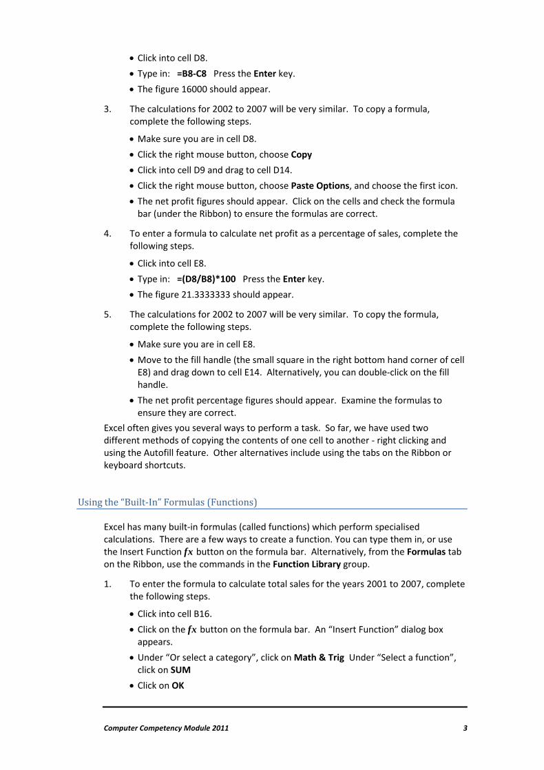
• Click into cell D8. • Type in: =B8-C8 Press the Enter key. • The figure 16000 should appear.

3. The calculations for 2002 to 2007 will be very similar. To copy a formula, complete the following steps.

• Make sure you are in cell D8. • Click the right mouse button, choose Copy • Click into cell D9 and drag to cell D14. • Click the right mouse button, choose Paste Options, and choose the first icon. • The net profit figures should appear. Click on the cells and check the formula

bar (under the Ribbon) to ensure the formulas are correct.

4. To enter a formula to calculate net profit as a percentage of sales, complete the following steps.

• Click into cell E8. • Type in: =(D8/B8)*100 Press the Enter key. • The figure 21.3333333 should appear.

5. The calculations for 2002 to 2007 will be very similar. To copy the formula, complete the following steps.

• Make sure you are in cell E8. • Move to the fill handle (the small square in the right bottom hand corner of cell

E8) and drag down to cell E14. Alternatively, you can double-click on the fill handle.

• The net profit percentage figures should appear. Examine the formulas to ensure they are correct.

Excel often gives you several ways to perform a task. So far, we have used two different methods of copying the contents of one cell to another - right clicking and using the Autofill feature. Other alternatives include using the tabs on the Ribbon or keyboard shortcuts.

Using the “Built-In” Formulas (Functions)

Excel has many built-in formulas (called functions) which perform specialised calculations. There are a few ways to create a function. You can type them in, or use the Insert Function fx button on the formula bar. Alternatively, from the Formulas tab on the Ribbon, use the commands in the Function Library group.

1. To enter the formula to calculate total sales for the years 2001 to 2007, complete the following steps.

• Click into cell B16. • Click on the fx button on the formula bar. An “Insert Function” dialog box

appears. • Under “Or select a category”, click on Math & Trig Under “Select a function”,

click on SUM • Click on OK


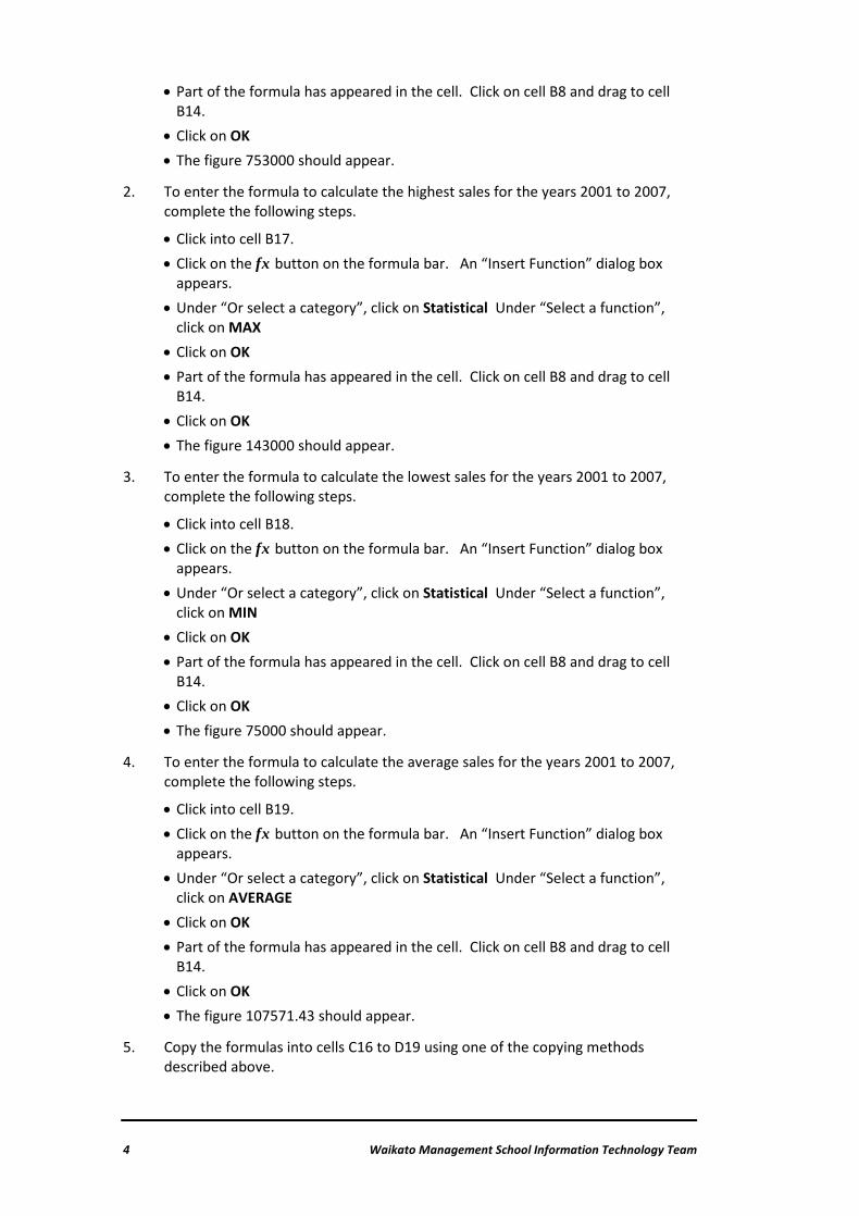
• Part of the formula has appeared in the cell. Click on cell B8 and drag to cell B14.

• Click on OK • The figure 753000 should appear.

2. To enter the formula to calculate the highest sales for the years 2001 to 2007, complete the following steps.


appears. • Under “Or select a category”, click on Statistical Under “Select a function”,

click on MAX • Click on OK • Part of the formula has appeared in the cell. Click on cell B8 and drag to cell

B14. • Click on OK • The figure 143000 should appear.

3. To enter the formula to calculate the lowest sales for the years 2001 to 2007, complete the following steps.



click on MIN • Click on OK • Part of the formula has appeared in the cell. Click on cell B8 and drag to cell

B14. • Click on OK • The figure 75000 should appear.

4. To enter the formula to calculate the average sales for the years 2001 to 2007, complete the following steps.



click on AVERAGE • Click on OK • Part of the formula has appeared in the cell. Click on cell B8 and drag to cell

B14. • Click on OK • The figure 107571.43 should appear.

5. Copy the formulas into cells C16 to D19 using one of the copying methods described above.


6. Save the file (click on the File tab and choose Save or click on the disk icon on the Quick Access toolbar).

Enhancing the Spreadsheet

In this exercise we will improve the appearance of the spreadsheet. You should still be in the file Happy_Harry.xlsx

Text

1. To bold the headings and change the font:

• Highlight the range A1 to E7. • Under the Home tab, within the Font group click on the Bold button on the

toolbar . • All the headings should be bolded.

2. With the same range still highlighted, under the Home tab, within the Font group change the font and size. Notice that you get a “live preview” of fonts and styles. When you move the mouse over a formatting button, "live preview" temporarily applies formatting to what you have selected.

3. Perform steps 1. and 2. on the range A16 to A19.

Centering Text Across Columns

1. To centre the heading across columns:

• Highlight the range A1 to E3. • From the Home tab, in the Alignment group click on the dialog box launcher.

A “Format Cells” dialog box appears. • Click on the Alignment tab and under “Horizontal” choose Center Across

Selection • Click on OK • The row cells are merged and the headings should centre across the selected

columns.

NB You can also highlight the text (one row at a time) and click on the button within the Alignment group under the Home tab.

Numbers

1. To change the way the numbers are shown, complete the following steps.

• Highlight the range B8 to D19. • Click the right mouse button, choose Format Cells • A “Format Cells” dialog box appears. Select the Number tab. • Under “Category” choose Number and under “Decimal places” choose 0 • Check the Use 1000 Separator (,) box. • Click on OK The numbers should now have commas and no decimal places.


2. Under the Home tab, in the Number group experiment with other number formats.

Borders And Patterns

1. To apply borders and patterns, complete the following steps.

• Highlight the desired range. • Click the right mouse button, choose Format Cells • A “Format Cells” dialog box appears. Select the Border tab and choose from

the options available. • Select the Fill tab and choose from the options available. • Click on OK

2. You can also change the borders and fill from the Home tab in the Font group. Experiment.

Formatting Shortcuts

We have covered some basic formatting features, such as changing the text, numbers, and using borders and patterns. Several formatting shortcuts are described below. In the file Happy_Harry.xlsx:

1. Once you have formatted a range of cells you can select the next range that you want to have the same “look” using the keyboard shortcut Ctrl+Y The previous format is repeated for the selected cells.

2. You can also copy cell formats with the Format Painter.

• Select the cell that has the format you want to copy.

• Click on the Format Painter button in the Clipboard group under the Home tab.

• Drag through the range where you want to paste the format. • The format is copied to the selected cells. • You can double-click the Format Painter button to apply the formatting to

multiple places in your spreadsheet.

3. Excel has some built-in combinations of formats or cell styles that you can apply or modify. A cell style is a defined set of formatting characteristics, such as fonts and font sizes, number formats, cell borders, and cell shading. To use these:

• Select the range of cells you want to format. • From the Home tab, in the Styles group choose Cell Styles • When you move the mouse over a cell style, "Live Preview", temporarily

applies formatting to what you have selected • Select a format by clicking on it. • The format is applied to the selected cells.

Similarly, Table Styles provide a way to quickly format an entire table using a preset style definition.


• Select the range of cells you want to format. • From the Home tab, in the Styles group choose Format as Table • Select a format by clicking on it. • Choose from the options available and click on OK • The table format is applied. • When you click into the table a Table Tools Design tab appears. In the Table

Style Options group you can turn different formatting elements on and off. • Experiment!

4. To clear the formats from a cell:

• Select the range of cells you want to “unformat”.

• From the Home tab, in the Editing group, click the Clear button and choose Clear Formats

• The cell formats are removed, but the data and formulas remain intact.

Exercise

• Practice applying, copying and clearing various formats.

Charts

A chart is a graphic representation of worksheet data. You can create either an embedded chart on a worksheet, or a chart sheet as a separate sheet in your file. If you change the data in your worksheet, the chart is updated to reflect the changes.

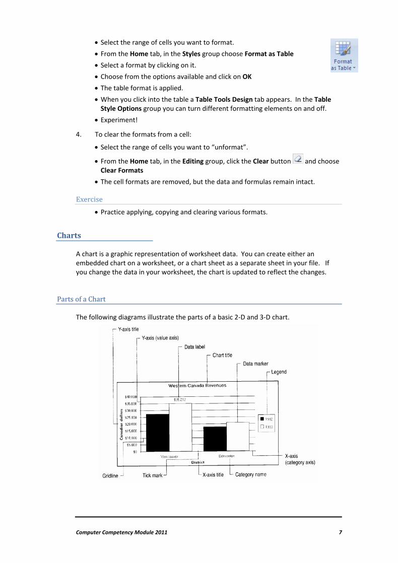
Parts of a Chart

The following diagrams illustrate the parts of a basic 2-D and 3-D chart.


(Source: Microsoft Excel 5 manual pp 270-271)

Creating a Chart

The first steps In the file Happy_Harry.xlsx. To create a column chart, complete the following steps: 1. Highlight the range B8 to D14. This is the data that you want to chart.

2. Click the Insert tab and from the Charts group click the Column button.

3. You will see a number of column chart types to choose from. Click the first column chart in the 2-D column list – the Clustered Column.

4. The chart appears.

5. Once your chart is inserted on the worksheet, the Chart Tools appear on the Ribbon with three tabs: Design, Layout, and Format. On these tabs, you’ll find various commands to work with charts.

Changing the Legend The chart legend (currently labelled Series1, Series2 and Series3) shows (by colour) which column represents the data (Sales, Total Expenses and Net Profit). To add the labels to the legend, complete the following steps:

1. Click on the chart to select it.

2. Click the Design tab, and from the Data group, click the Select Data button.


3. A “Select Data Source” dialog box appears.

• On the left hand side of the dialog box, ensure that Series1 is selected. • Click on the Edit button. • An “Edit Series” dialog box appears. • Click in the “Series name” box then click in cell B5 in the worksheet. Click on

OK • You should be back in the “Select Data Source” dialog box. • “Series1” should be replaced with “Sales”, and it should be visible in the

legend in the graph. • Ensure that Series2 is selected.

• Click on the Edit button. • An “Edit Series” dialog box appears. • Click in the “Series name” box then click in cell C5 in the worksheet. Click on

OK • You should be back in the “Select Data Source” dialog box. • “Series2” should be replaced with “Total Expenses”, and it should be visible

in the legend in the graph. • Ensure that Series3 is selected.

• Click on the Edit button. • An “Edit Series” dialog box appears. • Click in the “Series name” box then click in cell D5 in the worksheet. Click on

OK • You should be back in the “Select Data Source” dialog box. • “Series3” should be replaced with “Net Profit”, and it should be visible in the

legend in the graph.

4. Click on OK

Changing the x-axis The x-axis identifies the data being charted on the horizontal axis, in this case the years 2001 to 2007 (currently labelled 1 to 7). To add the correct labels to the x-axis, complete the following steps:

1. Click on the chart to select it.

2. Click the Design tab, and from the Data group, click the Select Data button.

3. A “Select Data Source” dialog box appears.

• On the right hand side of the dialog box (under Horizontal (Category) Axis Labels) click on the Edit button.

• An “Axis Labels” dialog box appears. • Click in the “Axis label range” box. • Select cells A8 to A14 in the worksheet. • Click on OK

• You should be back in the “Select Data Source” dialog box. • Click on OK


4. The years should appear under the x-axis.

Adding titles You can give a title to the chart itself, as well as to the chart axes to describe the chart data. It’s a good idea to add descriptive titles to your chart, so that readers don’t have to guess what the chart is about.

1. A chart title is a short summary of the information displayed. To add a chart title, complete the following steps:

• Click on the chart to select it. • Click the Layout tab, and from the Labels group, click the Chart Title button. • Select a location for the title. • A “Chart Title” text box appears in your chart. • In the “Chart Title” text box, type a description of your chart.

2. In charts, axes are the two lines that frame your data. The horizontal line is called the x-axis; the vertical line is called the y-axis. To add an axis title, complete the following steps:

• Click on the chart to select it. • Click the Layout tab, and from the Labels group, click the Axis Titles

button. • To create a title for your x-axis, select Primary Horizontal Axis Title

• Click on Title Below Axis • An “Axis Title” text box appears in the chart. • Type in “Years ending 31 March”

• To create a title for your y-axis, select Primary Vertical Axis Title • Choose the title location you want. • An “Axis Title” text box appears in the chart. • Type in “$”

NB A quick way to add chart titles is to click the chart to select it, and then go to the Design tab and the Charts Layout group. Click the More button to see all the layouts. Each option shows different layouts that change the way chart elements appear. Also, you can go the Layout tab, and from the Axes group, click the Axes button and choose from the options. Experiment!

Changing the Chart type You can change the chart type (say from a Column chart to a Line chart) after you create your chart. To change the chart type:

1. Click inside the chart to select it.

2. On the Design tab, within the Type group, click Change Chart Type, and then select another chart type.


Moving and Resizing a Chart

1. To move a chart, click on it to select it and drag it to the appropriate position.

2. To resize a chart:

• Click on it to select it. • Move to a selection handle (one of the back squares on the border) until the

mouse pointer changes to a double headed arrow. • Drag to the desired size.

3. To make a chart snap to the cell borders hold down the Alt key as you resize it.

Editing a Chart

1. To modify an embedded chart, you must select it. To do this, simply click in the chart.

2. To edit any aspect of the chart:

• Select an item by clicking on it (several clicks may be necessary to select a single item).

• Click the right mouse button and choose the desired option from the menu.

3. Other ways of editing a chart include using commands under the Design, Layout and Format tabs that appear when you select a chart. Practice editing the chart you created.

Trend Analysis in a Chart

To insert a trend line complete the following steps:

1. Activate the chart by clicking on it. (Make sure you have a line or column graph available.)

2. Click the Layout tab, and from the Analysis group, click the Trendline button.

3. Choose from the options available (eg a Linear trendline).

4. An “Add Trendline” dialog box appears.

• Choose the series you want to add a trendline to and click on OK

5. The trendline appears.

6. To format the trendline:

• Right-click on the trendline. • A “Format Trendline” dialog box appears. • Choose from the options and click on Close • The appropriate trend line and any equations should appear.


Exercise

• Practice adding trend lines to the data series using the various options.

Linking Chart Text to a Worksheet Cell

Linking chart text (for example a chart title, axis title, or text box) to a worksheet cell ensures any changes to the worksheet are reflected in the chart. To do this:

1. Select the title or text box on the chart.

2. Click into the formula bar and type: =

3. Select the worksheet cell you wish to link to.

4. Press the Enter key. The appropriate title should appear.

Exercise

• Practice linking the title on the chart to one of the headings on the basic info sheet of the Happy_Harry.xlsx file.

Copying a Chart

Copying Charts to Microsoft Word To copy a chart to another application (for example, Microsoft Word):

1. Click the chart to select it.

2. On the Home tab, in the Clipboard group, click the copy icon or right-click the chart and choose Copy

3. Switch to the Word document and click where you want the chart to appear.

4. Go to the Home tab, in the Clipboard group, click the lower half of the Paste button and choose Paste Special

• A “Paste Special” dialog box appears. • The various options are described under “Result” when you select them.

5. Choose an option and click on OK

6. The chart should appear.

Other Features

The following features are often useful.

Auditing a Spreadsheet

It is sometimes useful to be able to see the relationships in a spreadsheet, especially when things are not working as expected. Excel has several auditing features that can


track the flow of calculations on your spreadsheet by showing the precedents and dependants.

• Precedents are cells that are referred to by a formula in another cell. • Dependants are cells that contain formulas that refer to other cells.

In the file Happy_Harry.xlsx:

1. Click into cell D8. Go to the Formulas tab and within the Formula Auditing group click Trace Precedents An arrow appears that shows the cells that are referred to in cell D8.

2. Go to the Formulas tab and within the Formula Auditing group click Trace Dependants An arrow appears that shows the cells that depend on cell D8.

Exercise

• Experiment with other cells in the spreadsheet and with the other items in the Formula Auditing group.

Using the AutoFill feature

We have already used the AutoFill feature for copying data. It can also be used to enter a series.

1. Open the file autofill.xlsx This file contains several series. If column F shows ####### simply widen the column to see the contents.

2. To complete the list of months in column A:

• Highlight the range A2 to A3. • Move to the fill handle (the small square in the right hand corner of cell A3) and

drag down as many rows as you want to extend the list. • The months should appear in the appropriate format.

3. Experiment with the other lists in the file.

Inserting/Deleting Rows and Columns

1. To insert a column:

• Select a cell to the right of where you want to add a new column • From the Home tab, with the Cells group click the arrow next to (or under) the

Insert button and choose Insert Sheet Columns • A new column appears to the left of your insertion point.

2. To insert more than one column:

• Select the number of columns you want to insert by dragging across the column letter headings. Alternatively, to select multiple non-contiguous columns, hold down the Ctrl key and select each column.

• From the Home tab, with the Cells group click the arrow next to (or under) the Insert button and choose Insert Sheet Columns (or click the right mouse button and choose Insert)


• The new columns appear to the left of your selection.

3. To insert a row:

• Select a cell below where you want to add a new row. • From the Home tab, with the Cells group click the arrow next to (or under) the

Insert button and choose Insert Sheet Rows (or click the right mouse button and choose Insert)

• A new row appears above your insertion point.

4. To insert more than one row:

• Select the number of rows you want to insert by dragging across the row number headings. Alternatively, to select multiple non-contiguous rows, hold down the Ctrl key and select each row, or a cell in each row.

• From the Home tab, with the Cells group click the arrow next to (or under) the Insert button and choose Insert Sheet Rows (or click the right mouse button and choose Insert)

• The new rows appear above your selection.

5. To delete rows or columns:

• Select the row(s) or column(s) to be deleted. • From the Home tab, with the Cells group click the arrow next to (or under) the

Delete button and choose from the options available.

NB There is a difference between deleting and clearing rows or columns. Deleting a row or column completely removes it from the worksheet and moves adjacent rows or columns to close up the space. Clearing a row or column (from the

Home tab, in the Editing group, click the Clear button ) clears the contents (formulas and data) formats, notes, or all three from the row or column.

Inserting/Deleting Cells

1. To insert a cell or cells:

• Select a cell or cells. • From the Home tab, with the Cells group click the arrow next to (or under) the

Insert button and choose Insert Cells (or click the right mouse button and choose Insert)

• An “Insert” dialog box appears. • Select from the options and click on OK

2. To delete a cell or cells:

• Select a cell or cells. • From the Home tab, with the Cells group click the arrow next to (or under) the

Delete button and choose Delete Cells (or click the right mouse button and choose Delete)

• A “Delete” dialog box appears. • Select from the options and click on OK


NB Deleting a cell removes it from the worksheet and moves adjacent cells to close up the space. Clearing a cell (from the Home command tab, in the Editing group) clears its contents.

Using Sheets

A default file (called a workbook) has three worksheets, called Sheet1, Sheet2 etc You can:

• Rename the sheets • Insert or delete sheets • Move sheets (within the same workbook or to a different workbook) • Copy sheets (within the same workbook or to a different workbook) • Hide sheets • Colour sheets

1. To rename a sheet:

• Double click the sheet tab (or move to a tab, click the right mouse button and choose Rename)

• Type in an appropriate name.

2. To colour the name of a sheet:

• Move to the tab you want to colour, click the right mouse button and choose Tab Color

• Choose a colour.

3. To insert a sheet:

• Move to a sheet tab, click the right mouse button and choose Insert from the menu.

• An “Insert” dialog box appears. • Select Worksheet and click on OK • Alternatively:

• At the far right of all the worksheet tabs, click the Insert Worksheet button.

• A new worksheet is added to the right of all other worksheets. • Or:

• From the Home tab, with the Cells group click the arrow next to (or under) the Insert button and choose Insert Sheet

• Practice inserting several sheets using the methods described above.

4. To delete a sheet:

• Move to a sheet tab, click the right mouse button and choose Delete from the menu.

• A message appears. Click on Delete

5. To move a sheet within the same workbook, using the drag and drop method:

• Move to its tab, hold down the left mouse button and drag to a new position.


6. To move or copy a sheet to another workbook:

• Open the worksheet to be copied and the workbook to which it will be copied. • To display the worksheet that will be moved:

• Select the View tab. • In the Window group, click the Switch Windows button. • Select the workbook containing the worksheet to be moved. • Right click the Sheet tab of the worksheet to be copied. • Select Move or Copy... • The “Move or Copy” dialog box appears.

• To copy the worksheet into an existing workbook, from the To book: pull-down list, select the destination workbook.

• To copy the worksheet into a new workbook, from the To book: pull-down list, select (new book)

• From the Before sheet: scroll box, select where you want the worksheet copied. • NOTE: The sheet copy will be placed in front of the sheet you select.

• Tick Create a copy • Click OK • The worksheet is copied.

7. To hide a sheet:

• Click on a sheet tab to select it. • Click the right mouse button and choose Hide from the menu. • The sheet tab disappears.

8. To “unhide” a sheet:

• Click on a sheet tab to select it. • Click the right mouse button and choose Unhide • An “Unhide” dialog box appears. • Select the sheet you wish to show and click on OK

NB To select more than one sheet at a time, hold down the Ctrl key and click on the appropriate tabs.

“Freezing” Titles

Most worksheets are much larger than can be displayed on the screen at one time. Data can be hard to understand when titles at the top of the worksheet and descriptions at the left, scroll off the screen. To keep column or row titles in view while you are moving through a worksheet:

1. Move to the cell that marks the top left of the working area of the spreadsheet.

2. Go to View tab and from the Window group click on the Freeze Panes button and choose Freeze Panes


3. Now, everything above and to the left of that cell will always be visible, no matter where you are in the worksheet.

NB When you freeze panes, the Freeze Panes option changes to Unfreeze Panes so that you can unlock the frozen rows or columns

Cell References

So far, all the formulas we have created have used relative references. When cells containing relative references are copied, the column letters and row numbers adjust automatically. Absolute references are used to refer to a cell in an exact location. An absolute reference is created by adding a $ sign before the column letter and row number. When cells that contain absolute references are copied, the column letter and row number do not change. Cell references can also be mixed. A mixed reference is created by adding a $ sign before either the column letter or the row number, ie whichever part of the address you want to remain the same.

NB You can create absolute references without typing in the $ signs. After you type in the cell reference, press the F4 key and the relative reference changes to an absolute reference. To change the reference again, keep pressing the F4 key until the desired result is achieved.

Sorting Data

When you sort a list, the data in rows is rearranged according to the contents of the “Sort by” column that you choose.

1. Open the file SORTING.xlsx

2. To use the Sort feature to sort an entire list:

• Place the cursor somewhere in the list. • Go to the Data tab, and then within the Sort & Filter group click on the Sort

button. • The list is selected and a “Sort” dialog box appears. • To sort the students by their marks from the highest to the lowest:

• Under “Sort By” choose Mark, under “Sort On” choose Values and under “Order” choose Smallest to Largest

• Click on OK • The list is sorted.

Guidelines

• Excel identifies the column labels by looking at the formatting in the top rows of the list.

• If the sort was a mistake, use the Undo button in the Quick Access toolbar. • To sort by more than one column:

• When in the “Sort” dialog box, click the Add Level button.


• In the “Then by” row that appears, select your additional sort options • If you want to return a list to its original unsorted order, make sure you have a

column that numbers the rows, such as the OO (Original Order) column in the sample file. Then, when you want to return the list to the original order, sort by this column.

Exercises

1. Sort the students:

• By Sex • By Marks and Sex • Back to the original order

2. Explore the other options in the “Sort” dialog box.

Filtering Data in a List

AutoFilter allows you to display any data in a list that meets certain criteria. Any data not matching the specified criteria is hidden from view. Filtered data can be easily viewed again by removing the filter. Unlike sorting, filtering does not rearrange a list.

1. Open the file AUTOFILTER.xlsx

2. To use the AutoFilter feature:

• Place the cursor in the list you want to query. • Go to the Data tab, and then within the Sort & Filter group click on the Filter

button. • Arrows (called AutoFilter buttons) appear next to each heading in the list. • Select the list you want to use by clicking on its arrow - for example, click on the

arrow next to Grade • The list displays the various items in the column. • To filter the selected column, untick the items you do not want to show (for

example untick Fail) be sure that only the records you want displayed are selected).

• Click on OK • The list collapses so that only the records that meet that criterion (ie students

who passed) are displayed. The button next to the heading changes to a small version of the Filter command.

Guidelines

• You can choose from a range of filters, including number filters. • You can specify custom criteria for each column. Click on the arrow and choose

Number Filters, (or Text Filters depending on your data) Custom Filter • AutoFilter hides the rows that do not meet the criteria, so you should not put

other data in the same rows in the worksheet - note how the lookup table keeps disappearing!


• To remove a filter from a single column, click on small version of the Filter command. and choose Clear Filter From… (do this before starting the exercises below).

• To remove AutoFilter from the entire list, go to the Data tab, and then within the Sort & Filter group click on the Filter button.

Exercises Determine (using the Auto Filter):

• Those students who received a B grade • Those students who received the top 10 marks • Those students who received the bottom 10 marks • Those students who received either an A+ or an A++ grade (note that the A++

grade does not exist anymore – this is just an example) • Those students who were female and received an A+ grade

Close the file (no need to save).

Copying Data to Microsoft Word

To copy data to another application (for example, Microsoft Word):

1. In Excel, select some data.

2. On the Home tab, in the Clipboard group, click the copy icon or right-click the data and choose Copy

3. Move to the Word document and click where you want the data to appear.

4. Go to the Home tab, in the Clipboard group, click the lower half of the Paste button and choose Paste Special

• A “Paste Special” dialog box appears. The various options are described under “Result” when you select them. • Formatted Text (RTF) inserts the contents as text with font and table

formatting. • Unformatted Text inserts the contents as text without any formatting.

• Choose an option and click on OK

5. The data should appear.

Printing

For the following exercises, use any file you have been working with, follow the instructions and look at Print to preview the results. To get to the Print Preview window, go to the File tab and choose Print The “preview” is on the right hand side of the window.


General

1. Go to the File tab and choose Print

2. Check the print preview and choose from the settings to get the layout etc that you want. Click on Print

NB Page Layout view is useful to fine-tune the layout of your spreadsheet before printing. Go to the View tab, and from the Workbook Views group choose Page Layout When you want to return to the normal view, click on the Normal button in the Workbook Views group. Alternatively, use the icons on the right of the status bar.

Printing Part of a Spreadsheet

1. Select the range you want to print.

2. Go to the Page Layout tab and within the Page Setup group click the Print Area button and choose Set Print Area

• You can add more data to the print area by selecting a range of cells, clicking on the Print Area button and choosing Set Print Area

3. Print in the usual way.

NB To clear the print area, click on the Print Area button and choose Clear Print Area

Selecting Multiple Ranges Excel lets you print non-contiguous ranges, ie ranges that are not next to each other.

1. Select the first range to be printed.

2. Hold down the Ctrl key and select the next range to be printed, and repeat as necessary.

Print Titles

Print titles are the rows and columns in a spreadsheet that print at the top or left of every page. If you select a row for a title, it repeats at the top of every page. If you select a column for a title it repeats at the left of every page.

1. Go to the Page Layout tab and within the Page Setup group click the Print Titles button.

2. A “Page Setup” dialog box appears. You should be on the Sheet tab.

3. Under “Print Titles”, click into the appropriate box.

4. On the worksheet, select the rows or columns you want repeated on each page. (You may have to move the “Page Setup” dialog box out of the way.)


Printing With/Without the Gridlines Showing

1. Go to the Page Layout tab.

2. Within the Sheet Options group under Gridlines tick/untick the Print option.

Printing Everything on One Page

1. Go to the Page Layout tab and within the Scale to Fit group click the dialog box arrow.

2. A “Page Setup” dialog box appears. You should be on the Page tab.

3. Under “Scaling” choose Fit to: and ensure 1 appears in both boxes.

4. Click on OK

Centering on a Page

1. Go to the Page Layout tab and within the Page Setup group click on the Margins button.

2. Choose Custom Margins

3. A “Page Setup” dialog box appears. You should be on the Margins tab.

4. Under “Center on page” choose either Horizontally or Vertically

5. Click on OK

Headers and Footers

Headers and footers contain the text that prints at the top and bottom of each page. There are “built in” headers, or you can create your own.

1. Go to the Insert tab and from the Text group choose Header & Footer

2. The view changes to Page Layout view.

3. You can choose items for your header and footer from the buttons in the Header & Footer Elements group or type in your own details.

4. When you have finished, click back into the main body of your spreadsheet, go to the View tab, and from the Workbook Views group choose Normal, or click on the Normal view icon on the right-hand side of the status bar.


Printing a Chart

1. To print an embedded chart as part of a spreadsheet, simply include it in the range of data to be printed.

2. To print an embedded chart by itself on a page:

• Activate the chart by clicking on it. • Go to File tab button and choose Print • Check the way the chart is displayed on the page and make any changes using

the Page Setup link, then click on Print

Extra Notes

__________________________________________________________________

__________________________________________________________________

__________________________________________________________________

__________________________________________________________________

__________________________________________________________________

__________________________________________________________________

__________________________________________________________________

__________________________________________________________________

__________________________________________________________________

__________________________________________________________________

__________________________________________________________________

__________________________________________________________________

© 2011

The form and content of this document, as well as the accompanying materials, are copyright. For permission to reproduce all or part of this document please contact:

Monica van Oostrom

Waikato Management School IT Team

Waikato Management School

The University of Waikato

Private Bag 3105

Hamilton

email: [email protected]

Text finalised August 6, 2012

ms excel 2010 – an overview · pdf filewaikato management school - information...

Documents