MPRI M2 Internship report : Micro-F* in F*

Simon Forest, under the supervision of Catalin Hritcu, INRIA Paris

August 21, 2015

The general context

The F* project. F* [1, 13] is a joint project between INRIA and Microsoft Research. It is aimed atachieving three different goals at once: First, it is an OCaml-like functional programming language. Second, itis a verification system, like Why3 or Dafny, that is able to prove semi-automatically that a program satisfies acertain specification. Finally, it is a proof assistant, like Coq and Agda, that allows users to manually constructproofs and checks that these proofs are correct. As a tool aimed at achieving these three goals simultaneously,F* is the state of the art; related tools include Zombie/Trellys [5] and HTT [9].

As a proof assistant, F* provides a combination of SMT-based automation and constructive proofs, whichshould lead to more maintainable proofs compared to tactic proofs in Coq. The proofs in F* are typed functionalprograms, whereas in Coq they are produced by untyped imperative meta-programs written in Ltac. F* alsoprovides a semantic termination check based on a well-founded order on expressions; this check is much moreconvenient and flexible than syntactic termination checks e.g. in Coq. In particular, in F*, one can definecustom termination metrics, using lexicographic orders for instance, which leads to natural definitions andconcise proofs. However, F* became a proof assistant only very recently [13], so, at the moment, there are fewexamples of proofs written with it. The biggest example before this internship was the metatheory of SystemF-omega, which is only around 2000 lines of code.

Mechanized metatheory. The proofs of programming language metatheories are long and tedious, oftennot very deep and very easy to get wrong on paper. One can use proof assistants to help construct such proofsinteractively and mechanically check these proofs, following the POPLMark spirit [3].

The research problem

The question I have studied is whether a rich fragment of F* can be formalized within F* itself. This is aninteresting and challenging problem for two main reasons.

First, it gives a mechanized metatheory of F*, which is of first importance in order to gain confidence inthe use of F* as a verification tool. Also, the current metatheory is very complex and easy to get wrong, andis still work in progress. Until now, there were only paper proof sketches with a lot of holes, with some partsthat were not up-to-date, and with some serious errors. So there was a need to get all of this straight.

Second, it gives a mechanized metatheory in F*, which is also important in order to see what are the limitsand the capabilities of the F* tool. Until now, there were not many examples of F* used as a proof assistantand all these examples are quite small. Moreover, since F* has features that are not present in standard proofassistants, it was an opportunity to discover interesting proof patterns that are specific to F*. Finally, theextensive use of F* for such a big proof was also an opportunity to find bugs in the implementation.

Other attempts like this one have been done with other proof assistants, for example, Coq in Coq [4]. Butthis was new to F*; in the self-certification effort for the previous (a lot less expressive) F* variant [12] themetatheory was done in Coq and the verification effort was limited to producing Coq certificates [11].

Contributions

We have mechanically checked in F* most of the progress and preservation proofs for a rich subset calledmicro-F*, featuring dependent types and kinds, type operators, subtyping, subkinding, semantic terminationchecking, and a weakest-precondition calculus based on predicate transformers. Micro-F* is defined using 7mutually defined judgments (typing, subtyping, kinding, subkinding etc.) which are defined by a total ofalmost 100 rules. This mechanization became the largest case study of F* as a proof assistant. At the moment,the code is about 6500 lines of code.

During this process, we discovered effective proof patterns allowed by the features of F* that can be re-usedfor formalizing the metatheory of other programming languages. First, we defined parallel substitution in a

1

concise way using the lexicographic metrics of F* to show termination. Then, we proved a strong version ofthe substitution lemma [10], which is inspired by category theory [7, 8] and which entails many other usuallemmas, like weakening, bound strengthening, and the usual substitution lemma, that are usually proved oneby one in usual proofs about lambda-calculus. We also simplified a lot the paper preservation proof by usinga different induction scheme. Finally, we defined a generic inversion lemma, which entails all other inversionlemmas, and we used it extensively in the proof of progress. We have also used these patterns to simplify theproofs of the other mechanized metatheory examples in F*, such as STLC and λω.

The paper proof sketch of micro-F* was also fixed and improved by the experience acquired by the mech-anization: we fixed the proof of the substitution lemma, while finding a way to allow both CBV and CBNreductions in the operational semantics of pure expressions. Our solution involved significantly generalizingone of the logical validity rules of F*. We fixed the proof of the progress lemma by extending the definitionof values and adding some new reduction rules. We changed the way recursive functions are defined, using afixpoint operator instead of ‘let rec’, which is easier to handle in the mechanization. Finally, we fixed a lot ofsmall technical bugs in the rules of the language that were hard to detect in the paper proof sketch.

This experiment also brought about improvements to the F* tool. Indeed, during the proof, we found twopractical inconsistencies (ways to derive false from a consistent environment) that we filed as bugs and are nowfixed. Also, features were added in order to make this mechanization easier to work on: an interactive modeto work easily on a part of the code without having to verify all the code every time, and a way to focus oncases of a proof in order for the check to be quicker. Moreover, our efforts informed several new features weplan to add to the F* tool that could have been useful in the proofs, like a tactic language and a way to printthe proof context.

Arguments supporting its validity

The final result of this work is a mechanized proof of micro-F* in F*; this was considered valuable enough tobe part of a paper submitted to POPL 2016 [13]. Even though the correctness of the proof still depends on thecorrectness of F* itself, machine-checked proofs are generally considered more reliable than paper proofs [3].While we have already written the most interesting parts of the proof, we needed to admit some lemmas fortechnical reasons (e.g. current limitations in the F* tool), but we strongly believe that these lemmas are correct.

Conclusion and future work

To summarize, after proving such a big mechanized metatheory proof in F*, there are three main takeaways:First, F* can naturally express carefully designed lemmas and proofs, such that the category theory inspiredsubstitution lemma, which can greatly simplify the proofs. In particular, we often used functions and proofsthat have a non-trivial termination argument, often based on lexicographic metrics, and this allowed us towrite the most general version of functions and proofs and saved us a lot of time. Second, the constructiveproofs in F* are readable, easy to adapt to changes in definitions, and generally more maintainable than proofsmade with a tactic language. Third, while SMT-automation relieved us from a lot of tedious code one wouldhave to write manually in a prover like Coq, we found this kind of automation to be a mixed blessing. Whennot working correctly, there are few ways to get around the limitations. This explains why some proofs ofthis project could not be fully completed. In order to address this problem, a tactic language is planned to beadded to F*, in order to be able to write the proofs manually when the SMT-automation fails.

Several aspects of future work have been identified: Concerning F* as a proof assistant, adding an Mtac-inspired tactic language would increase completeness of the tool. Also, having a way to debug the proofs wouldbe useful. Finally, having an Agda-style editor mode would make writing proofs more convenient.

Concerning the metatheory of F*, a lot of work still remains to be done. In the short term, it would be niceto finish the last holes in our soundness proof for micro-F* and to extend this proof to bigger F* fragments(e.g. the lattice of effects, higher-order state, polymorphism, etc). In the medium term, the main goals areformally proving normalization and consistency for F*, and ideally machine checking these proofs (they arecurrently done only on paper and only for a small subset of F*), and also formalizing and proving the soundnessof the SMT encoding. In the long term, we are aiming for the self-certification of F* in F*, while still producingcertificates that can be checked by Coq in order to build strong confidence in the proofs [11].

2

1 Technical background

1.1 Overview of F* as a proof assistant

As a programming language, F* is an ML-like functional programming language with dependent typesand kinds, type operators, subtyping, subkinding, refinement types, inductive types, a lattice of effects and,most importantly, a weakest precondition calculus based on predicate transformers. The syntax F* expressionsis basically the same as Caml-light or F#. F* differs from these languages at the type and kind level. Inparticular F* allows programs to be given total or partial correctness specifications and includes a weakestprecondition calculus that produces proof obligations that are discharged using an SMT solver.

The type syntax of F* allows type-level lambda abstractions on expressions and types, and also type-levelapplications on expression and types.

In order to be able to write proofs with it, the type system includes a logical part with a validity judgmenton formulas. In this setting, formulas are types and types are formulas, which let the user mix the two whenmaking proofs. In particular, the type syntax includes usual logical operators like =⇒,∧,∨,∀.

In the next paragraph, we present the weakest precondition calculus used in F*.Weakest preconditions. Dijkstra [6] defines the semantics of programs as predicate transformers: func-

tions that produces preconditions on the input of the program from postconditions on the output of theprogram. This approach is inspired from Hoare logic, where the postcondition holds after the execution of theprogram on a state where the precondition is true. With predicate transformers, there are no specific precon-dition or postcondition, only a function that can build a precondition out of any postcondition, which happensto be more flexible in practice, but a bit less intuitive for humans. In the case of Dijkstra [6], the preconditionsproduced by the predicate transformer are weakest preconditions, that is, sufficient and necessary conditionssuch that the postconditions hold. Also, this was originally stated for an imperative language.

In the following, we denote wp(p, post) the weakest precondition for the program p such that the postcon-dition post holds after the execution.

One of the nice thing about this kind of predicate transformers is that the computation of the weakest-precondition behaves well on most of usual program syntax. For example, for a simple imperative languagethat acts on a heap, where preconditions and postconditions are just predicates written as formulas on thisheap:

• assignment: wp(x:=e, post) = post[e/x].

• sequencing: wp(p1; p2, post) = wp(p1, wp(p2, post)).

• conditional (where the if branch is executed when the guard is equal to 0, the else branch otherwise):wp(if e then p1 else p2, post) = (e=0 =⇒ wp(p1, post)) ∧ (e 6= 0 =⇒ wp(p2, post)).

For example: wp(if x-3 then x:=x+1 else x:=0, x=4) = (x-3 = 0 =⇒ x=3)∧(x-3 6= 0 =⇒ 0 = 4), which is equivalentto x = 3.

This setting can be changed a bit in order to work with a pure functional programming languages: ba-sically, the postconditions are now predicates on the values returned by expressions after computation, andpreconditions are predicates on the free-variables of the expression. For example, the weakest precondition forthe expression if y = 0 then 42 else -42 and the postcondition λ(x:int).x ≥ 0 (the predicate which tests whether thereturned value is positive) is y = 0.

As we have seen, the weakest precondition calculus let us compute the condition (that is, the precondition)with which a conclusion (that is, the postcondition) would be true. This can be used to build a verificationsystem. Indeed, if we want to prove a property of a program, that is a conclusion under certain premises, thenone can build the weakest precondition associated to the conclusion, and check, using for example SMT-solver,that the precondition is implied by the premises of the property.

Instead of using weakest precondition calculus as a tool to analyze a program from an outside point of view,one can try to directly integrate it in the programming language. In [14], a type system which includes thisweakest-precondition calculus in the typing judgment of expressions. This extension gives a structure of monadat the type level, which is called the Dijkstra monad. In more recent work on F* [13], this weakest preconditioncalculus is generalized to a lattice of effects including divergent, stateful and exception-throwing computations.At the end, the new typing judgment looks like this: Γ ` e : M t wp where M is the kind of computation (pure,divergent etc.), t the usual type, and wp the predicate transformer built from the weakest precondition calculus.These triples of three elements (monadic effect, type and WP) are called computation types. The WPs liveat the type level and should still be seen as functions from postconditions to preconditions, that also live atthe type level. And the built WPs let F* check the properties we want to show.

3

In order to verify something with a proof assistant, one needs to write definitions describing the conceptsinvolved, write the properties about these definitions, and write the proof of these properties. In F* there aretwo ways for this: a logical style and a constructive style.

Logical style. In the logical style, the verification process is devolved to the SMT-solver, which basicallyhave to check that some formulas are correct, imply other formulas etc. In this style, writing a definition iswriting a formula or an expression that computes something , writing a property is writing the formulas thatneed to be true or implied, and writing a proof is helping the SMT-solver to prove itself by adding in its contextalready-proved properties.

In order to introduce the properties we want to prove and their associated proofs in this style, we can usetwo mechanisms: intrinsic proofs and extrinsic proofs. With intrinsic proofs, we write the property wewant about an expression directly in the declaration of this expression. It is convenient for properties usedvery often, because one does not need use explicitly a lemma in order to get this property.

For example, if we want to specify that the usual append function on list that concatenates two lists l1 andl2 produces a list of length that is the sum of the two lists.

let rec append l1 l2 =match l1 with| [] → l2| a:l1’ → a:(append l1’ l2)

We first need to define what is the length of a list with a simple function:

let rec length l =match l with| [] → 0| x:l’ → 1+(length l)

Then we write the property we want to show. With intrinsic proofs, we specify the property in thedeclaration of the function, before the definition:

val append: #a:Type → l1:list a → l2:list a →Tot (list a) (requires True) (ensures (length (append l1 l2) = length l1 + length l2))

In this example, we declare a polymorphic function (on the variable a of kind Type) append that takes twolists as arguments and which is total (the Tot is a syntax-sugar notation for computation types that are totalcomputations), which does not require anything on the data (the requires part), and which ensures the propertyon lengths that we wanted (the ensures part). Now, every time append is used, the property about the lengthswill be added in the context and used transparently. Also, in this case, since the property we want to prove issimple, F* will be able to prove just with the code of append.

But intrinsic proofs are limited because they can only be chosen at declaration time, and because they canharm performance: the property is always added to the context even if it is not used.

We can also write extrinsic proofs that are separate from the definition. Using the same example, we canwrite the property on lengths in a extrinsic style like this:

val append property: #a:Type → l1:list a → l2:list a →Lemma (requires True) (ensures (length (append l1 l2) = length l1 + length l2))

let rec append property a l1 l2 =match l1 with| [] → ()| x:l1’ → append property l1’ l2

Here we declare the property we want to prove the same way we declare a function, except we return a Lemma

instead of a real type. And then we provide the body of the proof with a let, which can be recursive just likeusual let. As one can see, the proof is quite small, because F* is able to automate most of the reasoning: it canunfold itself the expressions appearing in the proof (in the example, the body of length and append are unfolded),it can reduce the expressions that are present, and it can use equalities in context to replace expressions byothers, and it can automate the small reasoning about arithmetics using the SMT-solver.

In general, the way to write proofs in F* is just to call the minimum number of lemmas at a particularpoint in order to introduce the needed properties into the context, then we let the SMT solver figure the detailsout. Note that we can only prove properties that involve pure expressions (that is, that F* already considersas pure). This is because F* does not allow impure expressions to appear at the type level, and that all thespecifications and properties we write live at the type level.

Constructive style. In the constructive style, the verification process is devolved to the type system. Inthis style, writing a definition is defining an inductive type, writing a property is declaring a function whichtakes terms of some types as arguments (the premises) and returns a term of some type (the conclusion), andwriting a proof is about writing an expression of the right type.

4

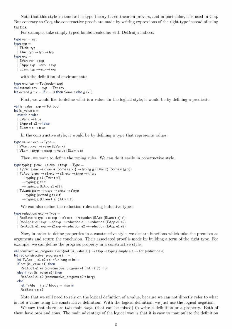
Note that this style is standard in type-theory-based theorem provers, and in particular, it is used in Coq.But contrary to Coq, the constructive proofs are made by writing expressions of the right type instead of usingtactics.

For example, take simply typed lambda-calculus with DeBruijn indices:

type var = nattype typ =| TUnit: typ| TArr: typ → typ → typ

type exp =| EVar: var → exp| EApp: exp → exp → exp| ELam: typ → exp → exp

with the definition of environments:

type env: var →Tot(option exp)val extend: env → typ →Tot envlet extend g t x = if x = 0 then Some t else g (x1)

First, we would like to define what is a value. In the logical style, it would be by defining a predicate:

val is value : exp →Tot boollet is value e =match e with| EVar x → true| EApp e1 e2 → false| ELam t e → true

In the constructive style, it would be by defining a type that represents values:

type value : exp →Type =| VVar : x:var → value (EVar x)| VLam : t:typ → e:exp → value (ELam t e)

Then, we want to define the typing rules. We can do it easily in constructive style.

type typing: g:env → e:exp → t:typ →Type =| TyVar: g:env → x:var{is Some (g x)} → typing g (EVar x) (Some.v (g x))| TyApp: g:env → e1:exp → e2: exp → t:typ → t’:typ→ typing g e1 (TArr t t’)→ typing g e2 t→ typing g (EApp e1 e2) t’

| TyLam: g:env → t:typ → e:exp → t’:typ→ typing (extend g t) e t’→ typing g (ELam t e) (TArr t t’)

We can also define the reduction rules using inductive types:

type reduction: exp →Type =| RedBeta: t: typ → e: exp → e’: exp → reduction (EApp (ELam t e) e’)| RedApp1: e1: exp → e2:exp → reduction e1 → reduction (EApp e1 e2)| RedApp2: e1: exp → e2:exp → reduction e2 → reduction (EApp e1 e2)

Now, in order to define properties in a constructive style, we declare functions which take the premises asarguments and return the conclusion. Their associated proof is made by building a term of the right type. Forexample, we can define the progress property in a constructive style:

val constructive progress: e:exp{not (is value e)} → t:typ → typing empty e t →Tot (reduction e)let rec constructive progress e t h =let TyApp e1 e2 t t’ hfun harg = ht inif not (is value e1) then

RedApp1 e1 e2 (constructive progress e1 (TArr t t’) hfunelse if not (is value e2) then

RedApp2 e1 e2 (constructive progress e2 t harg)elselet TyAbs t e t’ hbody = hfun inRedBeta t e e2

Note that we still need to rely on the logical definition of a value, because we can not directly refer to whatis not a value using the constructive definition. With the logical definition, we just use the logical negation.

We saw that there are two main ways (that can be mixed) to write a definition or a property. Both ofthem have pros and cons. The main advantage of the logical way is that it is easy to manipulate the definition

5

using logical operators, like negation, as we have seen for the value definition. On the other hand, reasoningabout it heavily relies on SMT-solver, which can fail to prove anything if the definitions or the properties aretoo complicated. It is hard to get the negation of a property defined by a constructive type, but it is easierto reason with: it is just about constructing and deconstructing terms, which needs less SMT-solving, so morethings can be proved in this way. Also inductive types are a very comfortable way to represent inference rulesof type systems, that will be useful for the work of this internship.

Termination. When defining lemmas or expressions that are total, F* needs to check that the computationterminates. In order to do it, a metric is defined on some of the types: for natural numbers, F* uses the classicaldecreasing metric, and for inductive types, a term of a certain type is considered lesser than another one ifthe former is a subterm of the latter. When defining a recursive function which is supposed to be total, F*will check that all the calls to the defined function are made with smaller arguments: by default, it checksthat the tuple of non-functional arguments decreases with a lexicographic ordering based on the metrics ofthe different types. But one can define other decreasing metrics on the tuples, by writing (decreases %[e1;...;en])where %[e1;...;en] defines a lexicographic metric using n expressions.

For example, take the Ackermann function:

val ackermann: n:nat →m:nat →Tot natlet rec ackermann n m =if m=0 then n + 1else if n = 0 then ackermann 1 (m 1)else ackermann (ackermann (n 1) m) (m 1)

F* will refuse this code, because it is not able to show that the arguments of ackermann decrease, based onthe default termination check mode. One can see that the recursive calls to ackermann are made with either asmaller m or with the same m but with a smaller n. So we can make F* understand that this code terminatesby specifying another lexicographic metric in the declaration:

val ackermann: n:nat →m:nat →Tot nat (decreases %[m;n])

Note that the expressions appearing in the user-defined lexicographic clauses can be any total expression.So we can write anything we want for them: one of the argument of the function, a computation returning atype with a metric (natural numbers for example), or even a non computable expression which still expresses aproperty of the arguments (for example, all0 f, which returns 0 if f x = 0 for all x, 1 otherwise). This terminationcheck also work with mutually defined functions: F* checks that the arguments of the calls to other mutualrecursive functions decrease. It can also be used with proofs and let the user define non-trivial induction.

1.2 Overview of micro-F*

Micro-F* is a sub-language of F* and shares a lot of features and concepts: monadic effects, WPs, typeoperators, subtyping, subkinding, logical fragment with types as formulas. One way to see it is as an extensionof λω. Even though it is only a fragment of F*, it is still very complex and hard to understand entirely. Sincemost of the ideas here are not specific to Micro-F*, the description of Micro-F* will stay high-level in thisreport. We only present some overview. The complete details can be found in [13].

Syntax. Micro-F* is based on three principal syntactic classes: expressions, types and kinds (as usual ina language with type operators). There is also syntax for computation types, which are tuples of 3 elements:a monadic effect (in this report, we will almost only talk about the PURE effect), a concrete type and a WP.The grammar for the syntax is presented in figure 1.

effects M ::= PURE | ALLexpression constants ec ::= () | n | h | l | bang | assign | select | update | fixpure | fixomega

expressions e ::= x | ec | e e | λx:t.e

values v ::= () | n | h | l | λx:t.e | partially applied constantstype constants tc ::= unit | int | heap | location | false | and | forallexpr | foralltype k | prectypes t ::= a | tc | t e | t t | t → c | λ x:t . t | λ a:k. t

kinds k ::= Type | x:t → k | a:k → k

computation types c ::= M t t

Figure 1: Syntax of micro-F?

Some details about this syntactic definition:

6

(Ps-Beta)

(λx : t.e) e′ → e[e′/x]

(Ps-LamT)

t→ t′

λx : t.e→ λx : t′.e

(Ps-FixPure)

fixpure e e′ v → e′ v (fixpure e e′)

(Ps-Update)

update h l i→ h[l→ i]

(Ps-Select)

select h l→ h[l]

(Ts-EBeta)

(λx : t.t′)e→ t′[e/x]

(Ts-TBeta)

(λa : k.t′)t→ t′[t/a]

(Ts-TLamT)

t→ t′

(λa : k.t)→ (λa : k.t′)

(Ts-TLamE)

t1 → t′1(λx : t1.t)→ (λx : t1.t)

(Ts-TAppE)

e→ e′

t e→ t e′

Figure 2: Reduction rules of micro-F?

• for expression constants: n are integers, h are heaps (functions from integers to integers), l are locationsin the heap (or references). bang and assign are the effectful functions to read and write references (sothey do not take heaps as argument). select and update are the pure functions to read and write in heaps(they take heaps as argument), and they are used to write properties of effectful computations at thetype level. fixpure and fixomega are the two fixpoint operators, one for pure computations and the otherfor effectful ones. They are parametrized by types that will define its type (since micro-F* does not havepolymorphism, it is a way to have polymorphic fixpoints).

• for type constants: false, and are the usual logical operators. forallexpr and foralltype are used to introduceda forall quantification for expressions and types at the logical level. prec is used to build inductiveinequalities between expressions.

• computation types: as we said earlier, are triples with an effect, a type for the result of the computation,and a WP, which is also encoded as a type. We will use the syntactic sugar Tot t to denote the computationtype PURE t wp, where wp requires the given postcondition to hold for all elements of the type.

• also note that we distinguish between expression variables and type variables, we have lambda-abstractionboth at the type and expression levels.

Reduction Micro-F* has reduction rules on both types and expressions, that are mutually recursive.We list here some of the most important reduction rules in figure 2. The definitions need to be mutuallyrecursive because of (Ps-LamT) and (Ts-TAppE). The reduction strategy of micro-F* involves both call-by-value (because of the fixpoint) and call-by-name (because of the β-reduction).

Type system. The type system is composed of 7 judgments that are mutually recursive:

• the typing judgment (figure 3), which assigns a computation type c for an expression e in an environ-ment Γ: Γ ` e : c. It may have been better to call it the computation judgment, but still it can be seenas an extension of the usual typing judgment. Sometimes in this report, to keep explanations simple, wewill do as if this judgment was only assigning a type to an expression, as in standard typing judgment forlambda-calculus. There are two specificities here. First, there are two application rules: since the typesystem asks for expressions that appear in types to be total, we have a rule checking that the argumentof the function is total when the arrow is dependent, which is T-App1. But when the arrow is notdependent, we allow applications of arguments that are not necessarily total with T-App2. Second, thereare two other rules that are not syntax directed and that only change the computation type part: thereis T-Sub which replaces the computation by a weaker one (according to a subcomputation judgment),and the T-Ret rule which acts only on total computations and returns a typing judgment where the WPis strengthened. Intuitively, the T-Ret rule allows the F* type system to reason about the concrete codeof pure expressions, not just about their type. We call these two rules the non-syntactic rules.

• the kinding judgment (figure 4), which assigns a kind k for a type t in an environment Γ: Γ ` t : k.The rules of this judgment are what one could expect from a lambda-calculus with subkinding and typeoperators.

• the kind well-formedness judgment, which establishes that a kind k is well-formed in an environment Γ:Γ ` k kwf . The definition of this judgment is not very interesting regarding what is following. It justchecks that the types appearing in the kind are kindable. We will not talk much about it.

7

(T-Var)

x : t ∈ ΓΓ ` x : Tot t

(T-Abs)

Γ ` t : Type Γ, x:t ` e : M t wp

Γ ` λx:t. e : Tot (x:t→M t wp)

(T-Const)

Γ ` ec : Tot (tec)

(T-App1)

x ∈ FV (t′) Γ ` e1 : M (x : t→M t′ wp) wp1 Γ ` e2 : Tot t

Γ ` e1 e2 : M (t′[e2/x]) (bindM wp1 λ .wp[e2/x])

(T-App2)

x 6∈ FV (t′) Γ ` e1 : M (x : t→M t′ wp) wp1 Γ ` e2 : M t wp2

Γ ` e1 e2 : M t′ (bindM wp1 (λ .bindM wp2 λx.wp))

(T-If0)Γ ` e0 : M int wp0 Γ ` e1 : M t wp1 Γ ` e2 : M t wp2

Γ ` if0 e0 then e1 else e2 : M t (iteM wp0 wp1 wp2)

(T-Sub)Γ ` e : M ′ t′ wp′ Γ `M ′ t′ wp′ <: M t wp

Γ ` e : M t wp(T-Ret)

Γ ` e : Tot tΓ ` e : PURE t (return t e)

Figure 3: Typing rules of micro-F?

(K-Var)

a : k ∈ ΓΓ ` a : k

(K-Const)

Γ ` tc : ktc

(K-Arr)

Γ ` t1 : Type Γ, x : t1 ` t2 : Type (some condition on wp)

Γ ` t1 →M t2 wp : Type

Figure 4: Some of the kinding rules of micro-F?

• the subtyping judgment (figure 5), which establishes that a type t’ is a subtype of a type t in an envi-ronment Γ: Γ ` t’ <: t. Note that it can not directly be used to apply subtyping in the typing judgment.Also note that we can get a subtyping relation from an equality at the logical level (validity judgmentbelow). So expression and type conversions are done in F* via subtyping and involve the SMT solver.

• the subkinding judgment, which establishes that a kind k’ is a subkind of a kind k in an environment Γ:Γ ` k’ <: k.

• the validity judgment (figure 6), which establishes that a formula (which is a type with kind Type)is logically true in an environment Γ: Γ |= φ. The validity judgment is essentially used to get typeequalities, that are used to build subtyping relations, and implications between WPs that are used tobuild subcomputation derivations. In the F* tool validity is discharged using the SMT solver.

• the subcomputation judgment (figure 7), which establishes that a computation type c’ is a subtype fromanother computation type c in an environment Γ: Γ ` c’ <: c. This is a judgment with only one rulewhich asks to prove that the type t’ in c’ is a subtype of the type t in c, and that the WP in c is “stronger”than the WP in c’.

The environment Γ contains expression variables (which are introduced by the typing judgment with ex-pression abstractions at the expression level, by the kinding judgment with expression abstractions at the typelevel etc. ) and type variables (which are introduced by the kinding judgment with type abstractions at thetype level, by the validity judgment with forall introduction etc. . . ). In order to say that the types and kindsin the environment are well defined, there is also a well-formedness judgment for environments.

Take away. In order to keep the explanations high level, but still to be able to imagine what were thechallenges faced when writing the proofs, we make the following summary.

First, about the main features of micro-F*: it is a lambda-calculus, of which λω can be seen as a fragment. It

(Sub-Conv)

Γ ` t1 : Type Γ ` t2 : Type Γ |= t1 =Type t2

Γ ` t1 <: t2

(Sub-Trans)

Γ ` t1 <: t2 Γ ` t2 <: t3Γ ` t1 <: t3

(Sub-Fun)

Γ ` t <: t′ Γ, x : t ` c′ <: c

Γ ` t′ → c′ <: t→ c

Figure 5: Subtyping rules of micro-F?

8

(V-Assume)

Γ ` e : tΓ |= t

(V-RedE)

e→ e′

Γ |= e = e′

(V-SubstE)

Γ |= e = e′ Γ |= φ[e/x]

Γ |= φ[e′/x]

(V-AndIntro)

Γ |= φ1 Γ |= φ2

Γ |= and φ1 φ2

(V-FalseElim)

Γ |= false Γ ` φ : Type

Γ |= φ

(V-ForallExpIntro)

Γ ` t : Type Γ, x : t |= φ

Γ |= forallexp(x : t).φ

(V-DistinctTH)

t1, t2 in head normal form t1 6= t2Γ |= not (t1 = t2)

Figure 6: Some validity rules of micro-F?

(SCmp)

M ′ ≤M Γ ` t′ <: t Γ |= wp =⇒ wp′

Γ |= M ′ t′ wp′ <: M t wp

Figure 7: Subcomputation rule of micro-F?

has more features, like subkinding, subtyping, a logical fragment . . . This calculus has expression variables andtype variables. It has expression and type variables because there are lambda abstraction at both expressionlevel and type level. Second, about the complexity of its specification. The specification of micro-F* is reallybig: 97 rules in total, more than a thousand lines in the code. It is also a challenge to write a proof about thiscalculus because both the syntactic forms and the judgments of the type system are mutually defined. So it isnot possible to handle what is going on at the kind level, then go to the type level then finish at the expressionlevel. Instead, a property on the type system needs to be proved mutually with all the judgments.

Additional formalization details. In order to write the proofs for this language in F*, different choicesof implementation were made.

First, the formalization uses a nameless representation of variables based on DeBruijn indices. The num-bering of expression variables and type variables are independent. As a consequence, we will stop showingnamed variables from here. For example, lambda abstraction will be denoted by λt.e instead of λx:t.e.

Also, environments are represented as a pair of two functions: one from variables to the types of micro-F*,and one from variables to the kinds of micro-F*. The result is returned using an option type, in case thevariables are not defined in the environment. When the environment are extended with other variables, itis always at the 0 position. Remember that the environment binds variables to types and kinds that canthemselves refer to variables of the environment. This implies that, when the environment is extended, thetypes and kinds in the environment must be shifted, that is, the free variables appearing in them must beincreased, in order to match the extended environment.

Finally, the judgments of the type system are written in F* using inductive types in order to write con-structive proofs. The reduction of terms is also represented with inductive types.

We refer the reader to the appendix (A.1) for the implementation details of the definitions.Goal. The goal of this internship was essentially to prove that micro-F* satisfies the progress and preser-

vation properties. We only attempted the proof for PURE computation types.

2 Substitution

In this section, we describe how we dealt with the definitions and the properties involving the generalnotion of substitution. We first explain how we defined the substitution of terms for micro-F* using parallelsubstitution. Then, we show how we extended this parallel substitution to the level of the type system to geta strong substitution lemma, which is needed for the preservation property among others.

2.1 Defining parallel substitution

Substitution is part of the formalization of micro-F*, since it appears in the type judgments and in thereduction relation. In order to simplify proofs, a concise and general definition of substitution was needed. Inthis section, we show how we defined substitution for micro-F* in detail, since it is a key component of the

9

formalization, and also because it shows some interesting termination problem that can be solved in F*. Wedefine parallel substitution functions that handle both expression and type variables.

We first define parallel substitution functions for each syntactic form, that is, a function that substitutesthe free variables inside expressions, types, kinds by expressions for expression variables and by types fortype variables. We substitute both expression variables and type variables at the same time. Since all thesyntactic forms are mutually defined, the parallel substitution functions are also mutually defined. There is asubstitution function for each syntactic form: esubst for expression substitution, tsubst for type substitution etc.Each of these functions takes two arguments:

• an argument s that we call a sub (for parallel substitution), which is a pair of functions, one from variablesto expressions (which we refer to with s.es), and one from variables to types (which we refer to with s.ts).This argument defines what will be substituted for the free variables met in the terms

• the syntactic form in which the substitution occurs

As one could imagine, these functions just go recursively on the structure of the terms, and when a freevariable is encountered, it is replaced by the corresponding element defined in the sub argument.

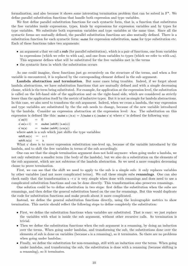
Lambda abstraction and termination. But some cases bring troubles. Indeed, if we forget aboutlambda abstractions, we have substitution functions that are mutually defined and with a simple decreasingclause, which is the term being substituted. For example, for application at the expression level, the substitutionis called on the left-hand side of the application and on the right-hand side, which are considered as strictlylesser than the application itself by the metric of inductive types. But it is not as simple for lambda abstractions.In this case, we also need to transform the sub argument. Indeed, when we cross a lambda, the way expressionand type variables are substituted by the the sub needs to change, because of the new variable introducedby the lambda. Consider an expression abstraction at the expression level: λt.e. The substitution on thisexpression is defined like this: esubst s (λt.e) = λ(tsubst s t).(esubst s’ e) where s’ is defined the following way:

s’.es(0) = 0s’.es(x+1) = esubst (eshift) (s.es(x))

s’.ts(a) = tsubst (eshift) (s.ts(a))

where eshift is a sub which just shifts the type variables:eshift.es(x) = x+1

eshift.ts(a) = aWhat s’ does is to move expression substitution one-level up, because of the variable introduced by the

lambda, and to shift the free variables in terms of the sub accordingly.One can see that the simple termination argument does not hold anymore: when going under a lambda, we

not only substitute a smaller term (the body of the lambda), but we also do a substitution on the elements ofthe sub argument, which are not subterms of the lambda abstraction. So we need a more complex decreasingclause to prove termination.

First, we can see that the shift we need to apply to the sub is a simple sub: it only replaces variablesby other variables (and not more complicated terms). We call these simple subs renamings. One can alsocheck easily that the transformation s → s’ is very simple when done with renamings and does need to use acomplicated substitution functions and can be done directly. This transformation also preserves renamings.

One solution could be to define substitution in two steps: first define the substitution when the subs arerenamings, and then define the general substitution based on the one for renamings. But this would duplicatethe code for substitution functions and make proofs about it more complicated.

Instead, we define the general substitution functions directly, using the lexicographic metrics to showtermination. This metric should reflect the following steps to define completely the substitution:

• First, we define the substitution functions when variables are substituted. That is easy: we just replacethe variables with what is inside the sub argument, without other recursive calls. So termination istrivial.

• Then we define the substitution functions when the sub argument is a renaming, by doing an inductionover the terms. When going under lambdas, and transforming the sub, the substitutions done over theelements of sub is done on variables (because s is a renaming), so it terminates. So there are no problemswhen going under lambdas.

• Finally, we define the substitution for non-renamings, still with an induction over the terms. When goingunder lambdas, and transforming the sub, the substitution is done with a renaming (because shifting isa renaming), so it terminates.

10

This induction was proposed by Altenkirch and Reus in [2]. At the end, we get the following decreasingclauses for the different functions:

• for esubst s e: [is evar e; is renaming s; e]

• for tsubst s t: [is tvar t; is renaming s; t]

• for ksubst s k: [1;is renaming s; k] (in the first position, there is a 1 because there are no variables at the kindlevel)

with is evar and is tvar functions that return 0 when their argument is a variable and 1 otherwise, andis renaming a function that returns 0 if its argument is a renaming, 1 otherwise.

let is evar e = if is EVar e then 0 else 1let is tvar t = if is TVar t then 0 else 1

type renaming (s:sub) = (forall (x:var). is EVar (Sub.es s x)) ∧ (forall (a:var). is TVar (Sub.ts s a))

let is renaming (s:sub) = if excluded middle (renaming s) then 0 else 1

Note that is renaming is not computable. It uses the function from F*’s classical logic library excluded middle

which is not defined, but only assumed as a function of this type:

val excluded middle: p:Type →Tot (b:bool{b = true ⇐⇒ p})

So excluded middle returns true if and only if the property passed as argument is true. When checkingtermination, F* will be able to do a case analysis on the result of excluded middle, that is, on whether thesubstitution is a renaming. So we are able to use it to finish our induction using this non-trivial property. Notealso that, once the decreasing clauses are given, the proof of termination is almost completely automated. Westill need to write some refinement types that concern renamings but that’s all.

Putting out the sub transformation. Now we have terminating mutually defined substitution functions.But there is still a problem: the sub transformation when going under lambdas is defined locally in thesubstitution functions and we can not refer to it from outside. Later, when we will want to prove some thingsabout this substitution, we will not be able to refer to this transformation:

let rec esubst s e =match e with...| ELam t e →(let s’ = (∗transformation of s to s’∗) inELam (tsubst s t) (esubst s’ e)

)(∗We can not refer to s’ from here, because it is a local variable∗)

One thing that can be done is to define again this transformation globally after the substitution functionsand prove that this global transformation does the same thing than the local transformation. But, due to F*limitations, this method slows down the verification process. So we need a better way.

A better way is to define this transformation mutually recursively with the 3 other substitution functions,instead of defining it locally every time a lambda is crossed. So we define sub elam (the transformation whengoing under expression lambdas) and sub tlam (the transformation when going under type lambdas) which takesone argument, which is the sub s on which the transformation is to be applied. The decreasing clauses needto be changed in order for the substitution functions to be able to call these transformations. That is, call tothe substitution functions need to be one level higher than the calls to the substitution transformations. Todo this, we simply add another parameter to the decreasing clause that will be 1 for the substitution functionsand 0 for the sub transformations.

At the end we get the following decreasing clauses:

• for esubst s e: [is evar e; is renaming s; 1; e]

• for tsubst s t: [is tvar t; is renaming s; 1; t]

• for ksubst s k: [1; is renaming s; 1; k]

• for sub elam s: [1; is renaming s; 0; (void)]

• for sub tlam s: [1; is renaming s; 0; (void)]

The last parameter of the decreasing clause is never relevant for termination of sub elam and sub tlam, whatis why it is replaced by void. This was a good example of an aspect of writing proofs with F*, which is findingthe right decreasing clause that makes the computation terminate.

11

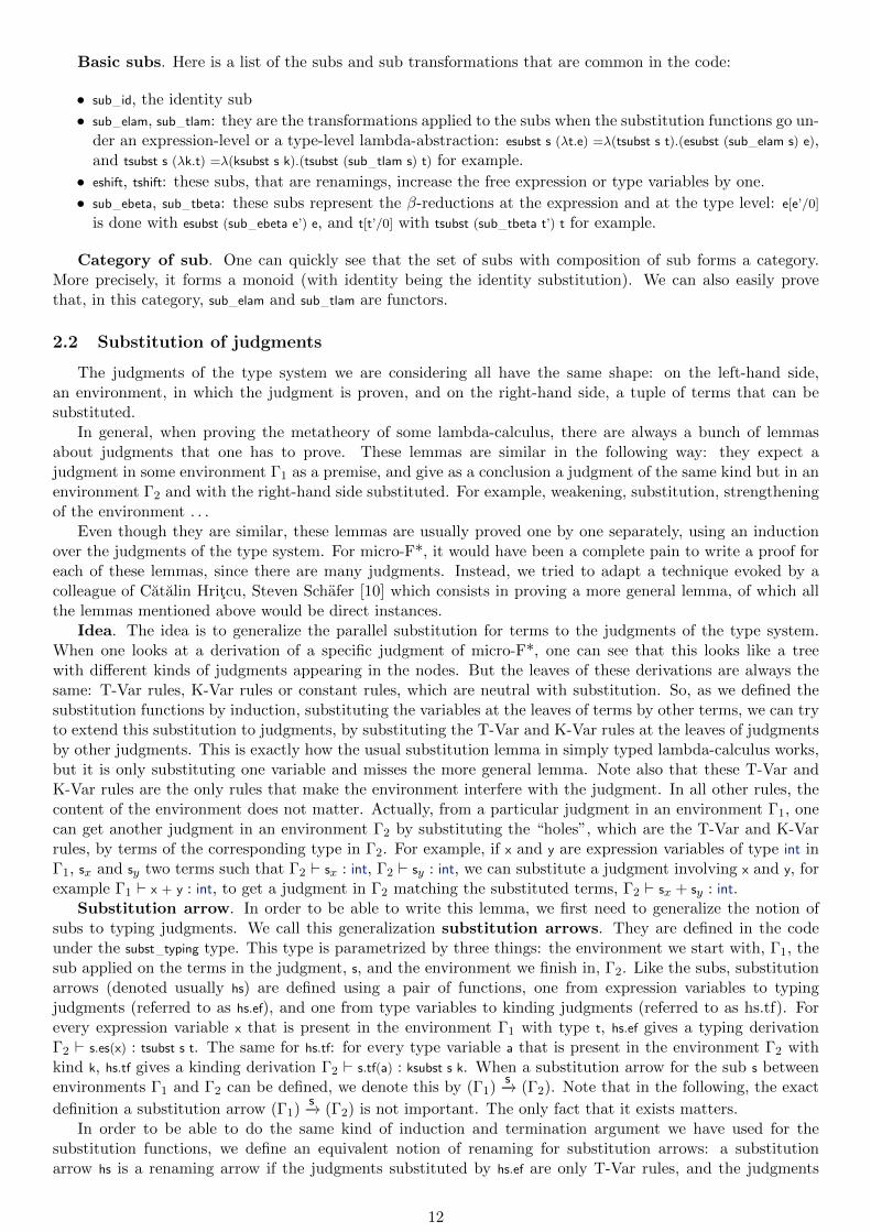
Basic subs. Here is a list of the subs and sub transformations that are common in the code:

• sub id, the identity sub

• sub elam, sub tlam: they are the transformations applied to the subs when the substitution functions go un-der an expression-level or a type-level lambda-abstraction: esubst s (λt.e) =λ(tsubst s t).(esubst (sub elam s) e),and tsubst s (λk.t) =λ(ksubst s k).(tsubst (sub tlam s) t) for example.

• eshift, tshift: these subs, that are renamings, increase the free expression or type variables by one.

• sub ebeta, sub tbeta: these subs represent the β-reductions at the expression and at the type level: e[e’/0]

is done with esubst (sub ebeta e’) e, and t[t’/0] with tsubst (sub tbeta t’) t for example.

Category of sub. One can quickly see that the set of subs with composition of sub forms a category.More precisely, it forms a monoid (with identity being the identity substitution). We can also easily provethat, in this category, sub elam and sub tlam are functors.

2.2 Substitution of judgments

The judgments of the type system we are considering all have the same shape: on the left-hand side,an environment, in which the judgment is proven, and on the right-hand side, a tuple of terms that can besubstituted.

In general, when proving the metatheory of some lambda-calculus, there are always a bunch of lemmasabout judgments that one has to prove. These lemmas are similar in the following way: they expect ajudgment in some environment Γ1 as a premise, and give as a conclusion a judgment of the same kind but in anenvironment Γ2 and with the right-hand side substituted. For example, weakening, substitution, strengtheningof the environment . . .

Even though they are similar, these lemmas are usually proved one by one separately, using an inductionover the judgments of the type system. For micro-F*, it would have been a complete pain to write a proof foreach of these lemmas, since there are many judgments. Instead, we tried to adapt a technique evoked by acolleague of Catalin Hritcu, Steven Schafer [10] which consists in proving a more general lemma, of which allthe lemmas mentioned above would be direct instances.

Idea. The idea is to generalize the parallel substitution for terms to the judgments of the type system.When one looks at a derivation of a specific judgment of micro-F*, one can see that this looks like a treewith different kinds of judgments appearing in the nodes. But the leaves of these derivations are always thesame: T-Var rules, K-Var rules or constant rules, which are neutral with substitution. So, as we defined thesubstitution functions by induction, substituting the variables at the leaves of terms by other terms, we can tryto extend this substitution to judgments, by substituting the T-Var and K-Var rules at the leaves of judgmentsby other judgments. This is exactly how the usual substitution lemma in simply typed lambda-calculus works,but it is only substituting one variable and misses the more general lemma. Note also that these T-Var andK-Var rules are the only rules that make the environment interfere with the judgment. In all other rules, thecontent of the environment does not matter. Actually, from a particular judgment in an environment Γ1, onecan get another judgment in an environment Γ2 by substituting the “holes”, which are the T-Var and K-Varrules, by terms of the corresponding type in Γ2. For example, if x and y are expression variables of type int inΓ1, sx and sy two terms such that Γ2 ` sx : int, Γ2 ` sy : int, we can substitute a judgment involving x and y, forexample Γ1 ` x + y : int, to get a judgment in Γ2 matching the substituted terms, Γ2 ` sx + sy : int.

Substitution arrow. In order to be able to write this lemma, we first need to generalize the notion ofsubs to typing judgments. We call this generalization substitution arrows. They are defined in the codeunder the subst typing type. This type is parametrized by three things: the environment we start with, Γ1, thesub applied on the terms in the judgment, s, and the environment we finish in, Γ2. Like the subs, substitutionarrows (denoted usually hs) are defined using a pair of functions, one from expression variables to typingjudgments (referred to as hs.ef), and one from type variables to kinding judgments (referred to as hs.tf). Forevery expression variable x that is present in the environment Γ1 with type t, hs.ef gives a typing derivationΓ2 ` s.es(x) : tsubst s t. The same for hs.tf: for every type variable a that is present in the environment Γ2 withkind k, hs.tf gives a kinding derivation Γ2 ` s.tf(a) : ksubst s k. When a substitution arrow for the sub s betweenenvironments Γ1 and Γ2 can be defined, we denote this by (Γ1)

s−→ (Γ2). Note that in the following, the exact

definition a substitution arrow (Γ1)s−→ (Γ2) is not important. The only fact that it exists matters.

In order to be able to do the same kind of induction and termination argument we have used for thesubstitution functions, we define an equivalent notion of renaming for substitution arrows: a substitutionarrow hs is a renaming arrow if the judgments substituted by hs.ef are only T-Var rules, and the judgments

12

substituted by hs.tf are only K-Var rules. So the effect on a typing derivation of this kind of arrow is to replaceT-Var leaves by other T-Var leaves, and K-Var leaves by other K-Var leaves.

Details specific to micro-F*. Once the idea is understood for a simple calculus, like the simply typedlambda-calculus, the following differences with micro-F* need to be emphasized: first, contrary to STLC, oreven λω, there is no stratification between the terms. There are all mutually recursive. The same for the typejudgments. So, contrary to STLC, where from a typing judgment we get another typing judgment where theonly thing which is replaced is the expression, here we substitute all the elements of the right hand side, sincefree variables can appear in any of them. Plus, remember that we have both expression variables and typevariables to handle. Also, we have to handle what the substitution does on the complicated encodings thatappear in the WPs in the computation types.

Statement and proof. Once we have defined these substitution arrows, we state how we can use them tosubstitute whole judgments. So, suppose we have built a substitution arrow (Γ1)

s−→ (Γ2). Then we have thefollowing statements on each kind of judgments:

Theorem 1. (Substitution lemma) If a substitution arrow (Γ1)s−→ (Γ2) can be built then the following state-

ments hold:

• Typing judgment: for e expression and c computation, if we have a derivation Γ1 ` e : c, then we canbuild the derivation Γ2 ` (esubst s e) : (csubst s e)

• Kinding judgment: for t type and k kind, if we have a derivation Γ1 ` t : k, then we can build thederivation Γ2 ` (tsubst s t) : (ksubst s k)

• Kind well formedness judgment: for k kind, if we have a derivation Γ1 ` k kwf , then we can build thederivation Γ2 ` (ksubst s k) kwf

• Subtyping judgment: for t’, t types, if we have a derivation Γ1 ` t’ <: t, then we can build the derivationΓ2 ` (tsubst s t’) <: (tsubst s t)

• Subkinding judgment: for k’, k kinds, if we have a derivation Γ1 ` k’ <: k, then we can build the derivationΓ2 ` (ksubst s k’) <: (ksubst s k)

• Validity judgment: for t type, if we have a derivation Γ1 |= t, then we can build the derivation Γ2 |=(tsubst s t)

• Subcomputation judgment: for c’, c computations, if we have a derivation Γ1 ` c’ <: c, then we can buildthe derivation Γ2 ` (csubst s c’) <: (csubst s c)

The proof of this big lemma needed different kinds of ingredients.First, since there are some substitutions appearing in the rules of the type judgment, and in the encodings

of WPs, we need to prove some commutation laws about the subs. For example, if Γ ` e1 : t→ t’ and Γ ` e2 : t,then, using dependent application, the final type is obtained with a substitution: Γ ` e1 e2 : t’[e2/0]. In thiscase, we need to show that substitution commutes well with the substitution on t’.

These proofs were completely carried out.Secondly, we need to prove that substitution of terms behaves nicely on encodings, that is to say that we

have some kind of morphism property on the encodings. For example, we need to prove that the tot function,which produces a computation for a type t which encodes the totalness property, verify the following property:csubst s (tot t) = tot (tsubst s t). These proofs were not carried out completely. The reasons for this are that theseproofs are generally tedious and non-interesting, that there are a lot of encodings that need proofs, and that itis difficult to write this proof to the end on complicated encodings, because at some point we reach a limitationwith the SMT automation. Still, these proofs help to find bugs in the encodings of the WPs that are done byend, in a DeBruijn fashion, that are very difficult to read and write.

Finally, we can write the big induction on all the judgments of the type system. The general way to writeeach case is to apply substitution on the premises, reapply by the constructor, and then use the morphismproperty of the encodings to conclude. But, as with substitution functions, we face some problems whengoing under a lambda. Indeed, when going under an expression or type lambda, the sub is transformed withsub elam or sub tlam, so we need to change the substitution arrow accordingly: we need to define a substitutionarrow transformation, as we have done for the subs. And, since there are substitutions happening duringthis transformation, we need to make these transformations mutually recursive, as before. We call these twotransformations elam hs and tlam hs.

13

Let’s see what transformation we need to write. So suppose we have a substitution arrow (Γ1)s−→ (Γ2) and

we are trying to substitute a T-Abs rule in the environment Γ1 into Γ2 with s : from Γ1 ` λt.e : t → t’ , wewant to build Γ2 ` esubst s (λt.e) : tsubst s (t → t’). (we just write the types instead of the whole computationtypes for clarity). By deconstructing the T-Abs rule in Γ1, one can get the judgment Γ1, t ` e : t’, and in orderbuild the conclusion in Γ2 with the T-Abs rule, one needs the judgment Γ2, tsubst s t ` esubst (sub elam s) e :tsubst (sub elam s) t’. We can see that we can get the latter judgment using the substitution lemma on the

former judgment with the substitution arrow (Γ1, t)sub elam s−−−−−−−→ (Γ2, tsubst s t). In order to conclude, we need

to build a substitution arrow transformation that builds a substitution arrow (Γ1, t)sub elam s−−−−−−−→ (Γ2, tsubst s t)

out of the substitution arrow (Γ1)s−→ (Γ2). We explain in detail how this transformation is done.

Lambda transformation We need to build a term hs’ that represents the arrow (Γ1, t)sub elam s−−−−−−−→ (Γ2, tsubst s t)

from the hs term. First, let’s build hs’.ef. In what follows, we denote ↑ the substitution with eshift, that is, theshifting of expression variables inside terms. There are two cases:

• for x = 0, we have that x is a variable of type t in (Γ1, t), so we need to give a derivation that(sub elam s).es(x), which is 0, is of type (tsubst s t) in (Γ2, tsubst s t) which is trivial.

• for x = n + 1, we have that x is a variable of type ↑ (t’) in Γ1, t, where x′ = n is a variable of type t′

in Γ1 (remember that an extended environment has its variables shifted). So we need build a derivationΓ2, (tsubst s t) ` (sub elam s).es(x) : tsubst (sub elam s)(↑ t’). Unfolding the definition of sub elam, and usinga commuting property with eshift this amounts to the derivation Γ2, (tsubst s t) `↑ (s.es(x’)) :↑ (tsubst s t’)But from hs.es(x’), we know a derivation Γ2 ` (s.es(x’)) : tsubst s t’. In order to conclude, we just need to

apply the substitution lemma on this last judgment with the substitution arrow (Γ2)eshift−−−−→ (Γ2, tsubst s t),

which we can easily build.

It is the same for hs’.tf. And we define the same way tlam hs. So we are able to correctly define thesetransformations, up to the termination check that gets trickier, as with substitution functions, that we solvethe same way.

We write the same kind of transformation for type lambdas. And this finish the global scheme of the proof.Deriving usual lemmas. We can now enjoy the power of our strong lemma and derive, painlessly, all the

interesting lemmas we want, just by providing a substitution arrow !

• Weakening: for t a type, we build the substitution arrow (Γ)eshift−−−→ (Γ, t) (this arrow is used in the proof

to build the lambda transformation)

• Substitution: for t a type, and e such that Γ ` e : Tot t, we build the substitution arrow (Γ, t)sub ebeta e−−−−−−−−→ (Γ)

• Supertyping in the environment: for t, t’ types such that Γ ` t’ <: t, we build the substitution arrow

(Γ, t)sub id−−−−→ (Γ, t′)

• Superkinding in the environment: basically the same than before but for kinds instead of types

So we get all the usual lemmas that were supposed to be proved one by one, with an induction eachtime. With this method, only one was necessary. And the amount of work that needs to be done to build asubstitution arrow is substantially lower than with an induction. And even the substitution arrows are flexible:if you want some other lemma which is a mix of the lemmas above, you can compose the existing substitutionarrows instead of writing a specific one.

A challenge. Writing this lemma was a challenge for several reasons. First, the general substitutionlemma was not part of the paper proof sketch. We turned to it because there were too many lemmas aboutsubstitution and they were not flexible enough.

The proof took a very long time to write (1 month) since it is an induction on all the judgments. At theend, this proof is 700 LoC.

Also, during this proof, the first F* limitations started to appear. First, as the proof went on, the verificationprocess took longer. Also SMT automation started to fail as the code got bigger. So a very awkward strategywas used to get around this: all the code for working cases was admitted. Only the case being written wasnot commented. Partly because of this awkwardness, an interactive mode was added to F* in order to avoidcompiling every time from the beginning. Also, an option was added in order to better handle big inductionson a lot of cases. Even with this feature, we could not make the proof completely work.

Some simplifications were also needed in order to make proofs easier to write. First, we changed the wayenvironment well-formedness was checked. In the paper proof version, environment well-formedness is another

14

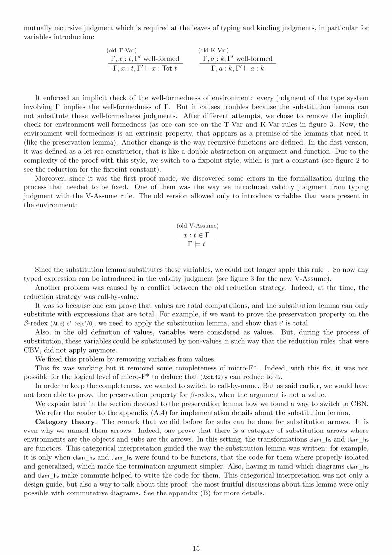
mutually recursive judgment which is required at the leaves of typing and kinding judgments, in particular forvariables introduction:

(old T-Var)

Γ, x : t,Γ′ well-formed

Γ, x : t,Γ′ ` x : Tot t

(old K-Var)

Γ, a : k,Γ′ well-formed

Γ, a : k,Γ′ ` a : k

It enforced an implicit check of the well-formedness of environment: every judgment of the type systeminvolving Γ implies the well-formedness of Γ. But it causes troubles because the substitution lemma cannot substitute these well-formedness judgments. After different attempts, we chose to remove the implicitcheck for environment well-formedness (as one can see on the T-Var and K-Var rules in figure 3. Now, theenvironment well-formedness is an extrinsic property, that appears as a premise of the lemmas that need it(like the preservation lemma). Another change is the way recursive functions are defined. In the first version,it was defined as a let rec constructor, that is like a double abstraction on argument and function. Due to thecomplexity of the proof with this style, we switch to a fixpoint style, which is just a constant (see figure 2 tosee the reduction for the fixpoint constant).

Moreover, since it was the first proof made, we discovered some errors in the formalization during theprocess that needed to be fixed. One of them was the way we introduced validity judgment from typingjudgment with the V-Assume rule. The old version allowed only to introduce variables that were present inthe environment:

(old V-Assume)

x : t ∈ ΓΓ |= t

Since the substitution lemma substitutes these variables, we could not longer apply this rule . So now anytyped expression can be introduced in the validity judgment (see figure 3 for the new V-Assume).

Another problem was caused by a conflict between the old reduction strategy. Indeed, at the time, thereduction strategy was call-by-value.

It was so because one can prove that values are total computations, and the substitution lemma can onlysubstitute with expressions that are total. For example, if we want to prove the preservation property on theβ-redex (λt.e) e’→e[e’/0], we need to apply the substitution lemma, and show that e’ is total.

Also, in the old definition of values, variables were considered as values. But, during the process ofsubstitution, these variables could be substituted by non-values in such way that the reduction rules, that wereCBV, did not apply anymore.

We fixed this problem by removing variables from values.This fix was working but it removed some completeness of micro-F*. Indeed, with this fix, it was not

possible for the logical level of micro-F* to deduce that (λx:t.42) y can reduce to 42.In order to keep the completeness, we wanted to switch to call-by-name. But as said earlier, we would have

not been able to prove the preservation property for β-redex, when the argument is not a value.We explain later in the section devoted to the preservation lemma how we found a way to switch to CBN.We refer the reader to the appendix (A.4) for implementation details about the substitution lemma.Category theory. The remark that we did before for subs can be done for substitution arrows. It is

even why we named them arrows. Indeed, one prove that there is a category of substitution arrows whereenvironments are the objects and subs are the arrows. In this setting, the transformations elam hs and tlam hs

are functors. This categorical interpretation guided the way the substitution lemma was written: for example,it is only when elam hs and tlam hs were found to be functors, that the code for them where properly isolatedand generalized, which made the termination argument simpler. Also, having in mind which diagrams elam hs

and tlam hs make commute helped to write the code for them. This categorical interpretation was not only adesign guide, but also a way to talk about this proof: the most fruitful discussions about this lemma were onlypossible with commutative diagrams. See the appendix (B) for more details.

15

3 Simple inversion scheme and preservation

In this section, we talk about the proof of the usual preservation lemma. One of the specificities of thislemma for micro-F* is that it handles both type-level reductions and expression-level reductions, since they aremutually-recursively defined. We will only give details about the proof for expressions. One of the contributionsof this internship was to simplify the proof of preservation lemma, and in particular, to remove the need towrite the complicated proofs of some lemmas called inversion lemmas.

Inversion lemmas. In STLC, when one has a judgment Γ ` e1 e2 : t, one knows that the last rule appliedis an application rule and can get directly that Γ ` e1 : t’→ t and Γ ` e2 : t’. And it is the same story for lambdaabstraction, variables introduction etc. So basically, one can reason about typing judgment syntactically: thelast rule applied only depends on the syntax of what is in the judgment.

In Micro-F*, things are not as simple. For the typing judgment, there can be up to three rules that producesthe same term, essentially because there are non-syntactic rules, which do not change the typed expression.So, when one has Γ ` e1 e2 : t in Micro-F*, one can not directly deconstruct and get the same judgments thanin STLC. But still, it would be nice to be able to reason syntactically. Which is the goal of inversion lemmas:to let one invert syntactically typing judgments.

In the paper proof, these inversion lemmas were used in the preservation lemma, because of the way theinduction was done. The preservation lemma (for typing judgments) takes a typing judgment Γ ` e : c and areduction step e→ e′ as arguments and returns a typing judgment Γ ` e’ : t as conclusion. In the paper proofof preservation, the induction was done on the reduction step, which is completely syntactic. So, this inductionneeds inversion lemmas, for all syntactic constructions at the expression level. And each one of them wouldhave been a difficult to write, because of what was needed for the WPs, which are a pain to handle in general.So inversion lemmas are basically a bad idea in Micro-F*

Induction on typing derivation. So, is it possible to avoid these inversion lemmas during the preserva-tion proof ?

The problem was present because of the gap between the induction on the reduction proof, which iscompletely syntactic, and the typing derivation, which has non-syntactic rules.

So one idea was to do an induction on the typing derivation instead of reduction in order to handle directlythe non-syntactic rules as one step of the induction.

But then how do we relate the induction on the typing derivation to the induction on the reduction ? For,this we do a three-level matching: first, a match on typing induction in order to handle the non-syntactic rules,then a match on the reduction term, and then a final match on the typing derivation. We do this in threesteps in order for F* to do some automation: after the first match, F* knows that the non-syntactic rules arealready handled. After the second match, F* knows what is the syntax of the expression. With these twoinformation, F* directly knows what is the last rule applied in the typing derivation. We show a piece of theproof that shows this three level match:

let rec pure typing preservation g e e’ t wp post hwf ht hstep hv = (∗ ht: the typing derivation, hstep: the reduction proof∗)match ht with| TySub ht’ hsc → ... (∗handling of TSub∗)| TyRet t htot → ... (∗handling of TRet∗)| → (

(∗ At this point, F∗ knows that ht is not built with TSub or TRet∗)match hstep with| PsBeta t e e’ →((∗At this point, F∗ knows that the typed expression is (\lambda t. e) e’ ∗)(∗And it can deduce that the last rule of the typing derivation is an application rule ∗)let TyApp htfuns htargs htotargs hktrets = ht in... (∗end of the proof for the beta case∗)

)| ... (∗other cases∗))

This induction with the typing derivation and this three-level matching simplified a lot the initial proof ofthe preservation lemma, and removed the need for almost all inversion lemmas (the PsBeta case still needs aninversion for lambda-abstraction) where the paper proof needs them.

But during the proof, we found that other cases (which were forgotten by the paper proof) needed inversionlemmas: the fully-applied expression constants, and each of them needed a specific inversion lemma.

We also found out that the inversion lemmas were needed in other places than the preservation lemma. Forexample, the progress proof needs them too.

16

So, even though we simplified the proof of the preservation lemma, the need for a lot of inversion lemmaswas still there.

Generic inversion lemma. But we can still try to avoid writing several inversion lemmas, by writinga generic inversion lemma that does not give the specific properties needed in each situation but allows tocompute them outside of this lemma out of more general properties it would return. In order to do this, wefirst make the following remark: the typing derivation of Γ ` e : c is a chain of non-syntactic rules (maybeempty) with a final typing rule which acts syntactically. For example, when we inductively go through thetyping derivation of Γ ` λt.e : c, we will first meet a number of T-Ret and T-Sub rules, and then we will hit aT-Abs rule.

Also, one can see that the information given by inversion lemmas can be derived from the informationcontained in the final syntactic rule and from the chain of non-syntactic rules.

So we just need to return these two pieces of information.In order to handle the first part, we need to represent typing derivations where the last applied rule is a

syntactic rule, that is, not a non-syntactic rule. We do this using F* refinements:ht:typing g e c{not(is TySub ht) && not (is TyRet ht)}.Note that we are using is TySub and is TyRet predicates that are automatically built by F* when defining

inductive types.In order to handle the second part, we define a type that represents the chain of non-syntactic rules that

we call scmpex for SubCoMPutationEXtended. This type is parametrized by four elements: the environment g,the typed expression e, and the two computations c and c’ that are at the borders of the chain.

The generic inversion lemma just builds and returns these two elements. And that’s all. Now, we can usethis lemma in all situations where inversion is needed and derive what we need in some specific case out ofwhat is returned. The interested reader can see more details in the appendix (see A.5).

Beta-reduction case. As we said earlier, the fix done to the values definition during the proof of thesubstitution lemma made F* less complete. In order to keep the same completeness, we wanted to switch toCBN.

But switching to CBN raises a problem in the preservation lemma proof because of the following facts:First, in order to prove the β-case ((λt.e) e’→e[e’/0]), one needs to use the substitution lemma. Second, thesubstitution lemma needs the expressions it substitutes with (e’ in the example) to be total.

But in general, expressions are not total. However, values are total. So we can prove the β-reduction casefor CBV but not for CBN.

In order to switch to CBN, we tried to find other conditions under which an expression was total. Weintroduced the notion of satisfiability of WPs at this point:

Definition 1. (Satisfiability) A WP wp is said to be satisfiable in the environment Γ if there exists a postcon-dition p such that the precondition wp post is satisfied in Γ : Γ |= wp p.

One can show as a first property that an expression typed with a satisfiable WP is total. Also, as a secondproperty, one can show that if the WP of an application e1 e2 is satisfiable, then the WP of e2 is satisfiable.

So, in order to use CBN anyway, we weakened the preservation lemma for expressions, and asked as premisethat the WP associated to the typing judgment is satisfiable.

With the two properties in mind, the new preservation property can be proved. Indeed, in the β-reductioncase (λt.e) e’, one can get the satisfiability of e’ with the premise, and deduce the fact that e’ is total. So we canapply the substitution lemma and conclude that e[e’/0] has the same computation type than (λt.e) e’.

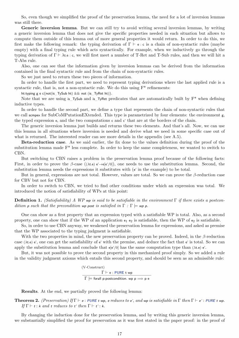
But, it was not possible to prove the second property in this mechanized proof simply. So we added a rulein the validity judgment axioms which entails this second property, and should be seen as an admissible rule:

(V-Construct)

Γ ` e : PURE t wp

Γ |= forall p:postcondition. wp p =⇒ p e

Results. At the end, we partially proved the following lemma:

Theorem 2. (Preservation) If Γ ` e : PURE t wp, e reduces to e’, and wp is satisfiable in Γ then Γ ` e’ : PURE t wp.If Γ ` t : k and t reduces to t’ then Γ ` t’ : k.

By changing the induction done for the preservation lemma, and by writing this generic inversion lemma,we substantially simplified the proof for preservation as it was first stated in the paper proof: in the proof of

17

the preservation lemma, we do not need anymore to apply an inversion lemma at each step. So we do not needanymore to prove difficult lemmas about WPs transformations that were needed before. These lemmas hadquit difficult proofs, were returning big and complicated types, were not flexible and were used only once. Sothis is a huge gain.

Also this design is generic enough to handled all situations where inversion is needed in Micro-F*. Plus,the complexity of the proofs are reduced since we only return a simple structure with a typing judgment anda scmpex in every case, instead of different complicated structures, which are all case specific So this design isreally useful and could be reused easily in other contexts.

Even with these new techniques, it was too difficult to write a complete proof. Even though most of thecases are handled, the most problematic one, which is the fix-point case, is not: the encoding of the type ofthe fix-point is too heavy to handle for F* at this point. Also, there are two holes in two other cases, dueto the difficulty to get a subkinding relation out of an expression/typing equality. For example, if we havea kind k with a free variable x and an equality judgment Γ |= e = e’, we need to build a subkinding relationΓ ` k[e/x] <: k[e’/ x]. Because of DeBruijn indices, this is actually very difficult, and we are still trying to figureout how to write a simple proof for it. Otherwise, the results are encouraging.

Also, during the proof, we were able to find a bug in the specification, which is that preservation does notnecessarily hold in an inconsistent environment.

The reader can refer to the appendix (A.6) for details of implementation.

4 Progress

We want to prove here the usual progress lemma: an expression which is typable in the empty environmentand which is not a value can be reduced.

The definition of values is quite heavy because of constants: every partial application of constants isconsidered as a value. Without automation, this would make the proof quite difficult since we would need toshow that all the non-values cases are handled by hand. But hopefully, F* is able to check automatically thatall the possible cases are handled.

The proof is done by induction on the typing derivation. Most of the cases for this match on the derivationare trivial: either we apply progress recursively (T-Sub, or T-Ret . . . ), or we return a simple reduction term(T-If0). The only difficult case is the application case e1 e2. There are different cases:

• if e1 is not a value, we apply progress recursively on e1

• if e2 is not a value, we apply progress recursively on e2

• if e1 is a lambda abstraction, we do a beta reduction

• otherwise, we are facing a fully applied constant

Fully applied constants are responsible for most of the work and the code on progress proof. Each one ofthem need to be treated individually. Here are the main cases:

• Pure fix-point: this is the easiest case since we do not need to check anything about the arguments andwe can directly apply the reduction step for fixpoint

• Pure operations: these are pure manipulations of heaps at the logical level. There are two operations:the select, which takes a heap and a location as arguments and returns the value in the heap at thislocation, and the update, which takes a heap, a location and an integer as arguments and returns themodified heap.

• Impure operations: these are constants that are not possible in a pure computation: the bang, whichreads a reference, the assign, which assigns an integer to a reference, and the impure fixpoint. But it isnot possible to remove these cases automatically. We need to show that such cases trigger a contradictionat the type-level.

The case of pure operations. What prevents us to apply the reduction step on these fully appliedconstants is that the reduction steps associated to these operations behave syntactically: the argument, that isexpected to be of type heap/integer/locations, needs to be a syntactic heap/integer/location. So, we proceedthe following way:

• we use inversion lemma to get the necessary information about the arguments of the fully applied con-stants: we build a typing judgment for each argument, such that the argument which is supposed to bea heap/integer/location at the end is typed as heap/integer/location.

18

• we show that, in the empty environment, a value of type heap/integer/location is a syntactic heap/inte-ger/location

These two points are not trivial and will be explained in detail in the next two paragraphs.Multiple Inversions for Application scheme. So, how do we show that the argument which is supposed

to be a heap/integer/location at the end can be typed as heap/integer/location ? In order to keep things simple,we will focus on only one example, which is the update constant. The only constraint about the argumentsof this constant is in the type of this constant, which is heap → location → int → heap (only the types ofcomputation types are written). We call this type the base type.

But relating the type of the constant to the type of the arguments is not simple, because of the subtypingrules that can be applied anywhere, and in particular on the constant. Since the subtyping relation includesbeta reduction at the type level, we can not even assume that we are handling an arrow type with threearguments at each step. The only thing we know about the shape of the handled types is that whenever anargument is applied to the (partially applied) constant, the type of the (partially applied) constant is t → t’

and the type of its argument is t. We call these types the upper types. What we want to do is to relate thebase type to the upper types. We do this in three steps (see figure 4):

• Unroll the type derivation of the fully applied constants, using the generic inversion lemma. This producesscmpex relations between the different upper types (the blue arrows on the figure)

• Hit the constant introduction and introduce the type for it (bottom of the figure)

• Apply back the arguments and use the subtyping relations in the scmpex to build a subcomputationrelation between the arguments types in the base type and the argument types in the upper types (redarrows on the figure), and also to get a subcomputation relation for the returned type (the green arrowon the figure)

Γ ` update e1 e2 e3 : t3

Γ ` update e1 e2 : ti → t3 Γ ` e3 : ti

Γ ` update e1 e2 : t2

Γ ` update e1 : tl → t2 Γ ` e2 : tl

Γ ` update e1 : t1

Γ ` update : th → t1 Γ ` e1 : th

Γ ` update : heap location int heap

Figure 8: Multiple inversions for application

Once we have the subtyping relation, we can apply subtyping to show that the arguments can be typedwith the right type.

This scheme, where one applies several times sequentially inversion lemmas to handle an application withseveral arguments, is used in other places, with something different each time. We call this design the multipleinversions for application scheme.

Getting syntactic heap/integer/location. So now we have values of type heap/integer/location. Howdo we prove that they are syntactically heaps/integers/locations ? The way we proceed is to handle all possiblesvalues and show that only one is possible, by reaching a contradiction in all other cases. The way we show acontradiction is to build a validity term of false in micro-F*, and use an axiom which raises the proof of falsein micro-F* to a contradiction at F* level: this axiom is basically the assumption that the empty environment

19

is consistent (that is, that you can not build a syntactic proof of false). Once false is in the context of theproof, we can finish the proof directly.

In order to show a contradiction, we go recursively in the typing derivation and we maintain an equalityproof term between the type we began with (heap/integer/location) and the type of the current subtree ofthe derivation, until we hit a rule which is not a non-syntactic one. Once we have this equality, we can usean axiom in the validity judgment which states that two types in normal form that are syntactically differentare different for the validity judgment. For example, if we start with e of type int, we maintain a judgment. |= t = int as we go recursively in the typing derivation of e. Then, we hit a rule which is not a subtyping one.There are different cases that are basically all the kinds of values we can encounter:

• if it is an integer introduction, we get the result of the lemma

• if it is a heap or a location introduction, we have an equality . |= t = int with t = heap or t = location fromwhich we deduce a contradiction

• if it is a lambda introduction, we have an equality . |= t1 → t2 = int which can be converted to acontradiction

• if it is a partially applied constant, one proves that the final type is equal to an arrow, which producesthe same contradiction than with lambda abstraction. In order to do this, a multiple inversions forapplication scheme is used, this time to relate the returned type at the base level to the returned type atthe upper level. For example, if we have a judgment . ` update e1 e2 : t, we show that . ` int→ heap <: t.From this, we can prove, using a helper lemma, that t itself is equal to an arrow type t1 → t2, and, bytransitivity, t1 → t2 = int and we get a contradiction.

Once we proved this lemma, we can do a reduction step on update and select operations.The case of impure computations. There are still one case left in the proof of progress, which are the

fully applied constants that lead to impure computations. For this paragraph, we introduce back the notionof effect of computations. The idea for this case is to do again a multiple inversions for application scheme inorder to get the fact that an effectful computation is a subcomputation of a pure one. For example, for theassign operation: the assign operation has the following type: location → int → ALL unit wp. When we have atyping derivation . ` assign e1 e2 : c, where c = PURE t wp’, we use the multiple inversions for application schemeto get a subcomputation term: . ` ALL unit wp <: PURE t wp’, which is impossible since the subcomputationconstructor prevents syntactically an effectful computation to be a subcomputation of a pure computation.This introduces the contradiction in F* and let us finish the proof.

Results. At the end, we were able to almost completely prove the progress lemma:

Theorem 3. (Progress) If Γ ` e : c and e is not a value then e reduces to some e’.

Contrary to the preservation proof, all the cases are handled. But the proof still relies on lemmas aboutWPs that are partially proved. This proof was also an occasion to develop several variants of the multipleinversions for application scheme, and a way to test the flexibility of the generic inversion lemma. The resultsare quite satisfying and it should make the case for reusing these schemes in other proofs about programminglanguages.

We also fixed the metatheory of micro-F*: at some point, the select and update constants were not reduciblewhen fully applied (so Ps-Select and Ps-Update did not exist). They were just used at the logical level andthe the properties about them were axioms at the logical level.

But still, when fully applied, select would produce a value of type int. This made the following typableexpression not reducible: if select h l then e else e’, which is not a value and so breaks the progress lemma. So weintroduced reduction rules for select and update in order to fix the problem.

We refer the reader to the appendix (A.7) for implementation details.

Conclusion

Due to space constraint, we refer the reader to page 2 for a summary of contributions and future work.

20

A Pieces of code of the project

A.1 Definitions of terms

type eff =| EfPure| EfAll

type econst =| EcUnit| EcInt : i:int → econst| EcLoc : l:loc → econst| EcBang| EcAssign| EcSel| EcUpd| EcHeap : h:heap → econst| EcFixPure : tx:typ → t’:typ → t’’:typ →wp:typ → econst| EcFixOmega : tx:typ → t’:typ →wp:typ → econst

and tconst =| TcUnit| TcInt| TcRefInt| TcHeap

| TcFalse| TcAnd

| TcForallE| TcForallT : k:knd → tconst

| TcEqE| TcEqT : k:knd → tconst

| TcPrecedes

and knd =| KType : knd| KKArr : karg:knd → kres:knd → knd| KTArr : targ:typ → kres:knd → knd

and typ =| TVar : a:var → typ| TConst : c:tconst → typ

| TArr : t:typ → c:cmp → typ| TTLam : k:knd → tbody:typ → typ| TELam : t:typ → tbody:typ → typ| TTApp : t1:typ → t2:typ → typ| TEApp : t:typ → e:exp → typ

and exp =| EVar : x:var → exp| EConst : c:econst → exp| ELam : t:typ → ebody:exp → exp| EIf0 : eguard:exp → ethen:exp → eelse:exp → exp| EApp : e1:exp → e2:exp → exp

and cmp =| Cmp : m:eff → t:typ →wp:typ → cmp

A.2 Definitions of reduction

type tstep : typ → typ →Type =| TsEBeta : tx:typ →

t:typ →e:exp →tstep (TEApp (TELam tx t) e) (tsubst ebeta e t)

| TsTBeta : k:knd →

21

t:typ →t’:typ →tstep (TTApp (TTLam k t) t’) (tsubst tbeta t’ t)

| TsArrT1 : #t1:typ→#t1’:typ→c:cmp →=ht:tstep t1 t1’ →tstep (TArr t1 c) (TArr t1’ c)

| TsTAppT1 : #t1:typ →#t1’:typ →t2 : typ →=ht:tstep t1 t1’ →tstep (TTApp t1 t2) (TTApp t1’ t2)

| TsTAppT2 : t1:typ →#t2:typ →#t2’:typ →=ht:tstep t2 t2’ →tstep (TTApp t1 t2) (TTApp t1 t2’)

| TsEAppT : #t:typ →#t’:typ →e:exp →=ht:tstep t t’ →tstep (TEApp t e) (TEApp t’ e)

| TsEAppE : t:typ →#e:exp →#e’:exp →=he:epstep e e’ →tstep (TEApp t e) (TEApp t e’)

| TsTLamT : k:knd →#t:typ →#t’:typ →=ht:tstep t t’ →tstep (TTLam k t) (TTLam k t’)

| TsELamT1 : #t1:typ →#t1’:typ →t2:typ →=ht:tstep t1 t1’ →tstep (TELam t1 t2) (TELam t1’ t2)

and epstep : exp → exp →Type =| PsBeta : t:typ →

ebody:exp →e:exp →epstep (EApp (ELam t ebody) e) (esubst ebeta e ebody)

| PsIf0 : e1:exp →e2:exp →epstep (EIf0 (eint 0) e1 e2) e1

| PsIfS : i:int{i<>0} →e1:exp →e2:exp →epstep (EIf0 (eint i) e1 e2) e2

| PsAppE1 : #e1:exp →#e1’:exp →e2:exp →=ht:epstep e1 e1’ →epstep (EApp e1 e2) (EApp e1’ e2)

| PsAppE2 : e1:exp →#e2:exp →#e2’:exp →=ht:epstep e2 e2’ →epstep (EApp e1 e2) (EApp e1 e2’)

| PsLamT : #t:typ →#t’:typ →ebody:exp →=ht:tstep t t’ →epstep (ELam t ebody) (ELam t’ ebody)

| PsIf0E0 : #e0:exp →#e0’:exp →ethen:exp →eelse:exp →=ht:epstep e0 e0’ →

22

epstep (EIf0 e0 ethen eelse) (EIf0 e0’ ethen eelse)| PsFixPure : tx:typ → t’:typ → t’’:typ →wp:typ →

d:exp → f:exp → v:value →epstep (eapp3 (EConst (EcFixPure tx t’ t’’ wp)) d f v)(eapp2 f v (eapp2 (EConst (EcFixPure tx t’ t’’ wp)) d f))

| PsUpd : h:heap → l:loc → i:int →epstep (eapp3 (EConst EcUpd) (eheap h) (eloc l) (eint i)) (eheap (upd heap l i h))

| PsSel : h:heap → l:loc →epstep (eapp2 (EConst EcSel) (eheap h) (eloc l)) (eint (h l))

A.3 Definition of type system

type typing : env → exp → cmp →Type = (∗typing judgment∗)

| TyVar : #g:env → x:var{is Some (lookup evar g x)} →typing g (EVar x) (tot (Some.v (lookup evar g x)))

| TyConst : g:env → c:econst → ecwf g c →typing g (EConst c) (tot (econsts c))

| TyAbs : #g:env →#t1:typ →#ebody:exp →m:eff →t2:typ →wp:typ →=hk:kinding g t1 KType →typing (eextend t1 g) ebody (Cmp m t2 wp) →typing g (ELam t1 ebody) (tot (TArr t1 (Cmp m t2 wp)))

| TyIf0 : g:env → e0 : exp → e1:exp → e2:exp →m:eff →t:typ →wp0 : typ →wp1 : typ →wp2:typ →typing g e0 (Cmp m tint wp0) →typing g e1 (Cmp m t wp1) →typing g e2 (Cmp m t wp2) →typing g (EIf0 e0 e1 e2) (Cmp m t (ite m t wp0 wp1 wp2))

| TyApp : #g:env →#e1:exp →#e2:exp →#m:eff →#t:typ →#t’:typ →#wp:typ →#wp1:typ →#wp2:typ →=ht1:typing g e1 (Cmp m (TArr t (Cmp m t’ wp)) wp1) →

=ht2:typing g e2 (Cmp m t wp2) →=htot:option (typing g e2 (tot t)){teappears 0 t’ =⇒ is Some htot} →=hk:option (kinding g (teshd t’) KType){not (teappears 0 t’) =⇒ is Some hk} →

typing g (EApp e1 e2) (Cmp m (tsubst (sub ebeta e2) t’) (tyapp wp m e2 t t’ wp wp1 wp2))

| TyRet : #g:env →#e:exp → t:typ →typing g e (tot t) →typing g e (Cmp EfPure t (return pure t e))

| TySub : #g:env →#e:exp →#c’:cmp →#c:cmp →=ht:typing g e c’ →=hsc:scmp g c’ c →

typing g e c

and scmp : g:env → c1:cmp → c2:cmp →Type = (∗subcomputation judgment∗)

| SCmp : #g:env →m’:eff →#t’:typ →wp’:typ →m:eff{eff sub m’ m} →#t:typ →wp:typ →=hs:styping g t’ t →=hk:kinding g wp (k m m t) →=hvmono:validity g (monotonic m t wp) →=hk’:kinding g wp’ (k m m’ t’) →=hvmono’:validity g (monotonic m’ t’ wp’) →

=hvsub :validity g (sub computation m t wp m’ t’ wp’) →scmp g (Cmp m’ t’ wp’) (Cmp m t wp)

and styping : g:env → t’:typ → t:typ →Type = (∗subtyping judgment∗)| SubConv : #g:env →#t:typ → t’:typ →

=hv:validity g (teqtype t’ t) →

23

=hk:kinding g t KType →=hk’:kinding g t’ KType →

styping g t’ t

| SubFun : #g:env →#t:typ →#t’:typ →#c’:cmp →#c:cmp →=hst:styping g t t’ →=hsc:scmp (eextend t g) c’ c →

=hk’:kinding g (TArr t’ c’) KType →styping g (TArr t’ c’) (TArr t c)

| SubTrans : #g:env →#t1:typ →#t2:typ →#t3:typ →=hs12:styping g t1 t2 →=hs23:styping g t2 t3 →

styping g t1 t3and tcwf : g:env → tc:tconst →Type = ... (∗type constant wellformedness∗)and ecwf : g:env → ec:econst →Type = ... (∗expression constant wellformedness∗)and kinding : g:env → t : typ → k:knd →Type =

| KVar : #g:env → x:var{is Some (lookup tvar g x)} →kinding g (TVar x) (Some.v (lookup tvar g x))

| KConst : #g:env →#c:tconst →tcwf g c →kinding g (TConst c) (tconsts c)

| KArr : #g:env →#t1:typ →#t2:typ →#phi:typ →#m:eff →=hk1:kinding g t1 KType →=hk2:kinding (eextend t1 g) t2 KType →=hkp:kinding (eextend t1 g) phi (k m m t2) →=hv :validity (eextend t1 g) (monotonic m t2 phi) →

kinding g (TArr t1 (Cmp m t2 phi)) KType

...

and skinding : g:env → k1:knd → k2:knd →Type= ... (∗subkinding judgment ∗)and kwf : env → knd →Type = ... (∗kind wellformedness ∗)and validity : g:env → t:typ →Type = (∗validity judgment∗)

| VRedE : #g:env →#e:exp →#t:typ →#e’:exp →=ht :typing g e (tot t) →=ht’:typing g e’ (tot t) →=hst:epstep e e’ →

validity g (teqe t e e’)

| VSubstE : #g:env →#e1:exp →#e2:exp →#t’:typ → t:typ →=hv12 :validity g (teqe t’ e1 e2) →=ht1 :typing g e1 (tot t’) →=ht2 :typing g e2 (tot t’) →=hk :kinding (eextend t’ g) t KType →=hvsub:validity g (tsubst ebeta e1 t) →

validity g (tsubst ebeta e2 t)

| VForallIntro : #g:env →#t:typ →#phi:typ →=hk:kinding g t KType →=hv:validity (eextend t g) phi →

validity g (tforalle t phi)

| VAndIntro : #g:env →#p1:typ →#p2:typ →=hv1:validity g p1 →=hv2:validity g p2 →

validity g (tand p1 p2)

| VFalseElim : #g:env →#t:typ →=hv:validity g tfalse →=hk:kinding g t KType →

validity g t

24

| VDistinctTH : #g:env →#t1:typ{is hnf t1} →#t2:typ{is hnf t2 && not (head eq t1 t2)} →

=hk1:kinding g t1 KType →=hk2:kinding g t2 KType →

validity g (tnot (teqtype t1 t2))

We also define a judgment for the well-formedness of environments:

type ewf : env →Type =

| GEmpty : ewf empty

| GType : #g:env →#t:typ →=hw:ewf g →=hk:kinding g t KType →

ewf (eextend t g)

| GKind : #g:env →#k:knd →=hw:ewf g →=h:kwf g k →

ewf (textend k g)

A.4 Substitution of judgments

We first define in the code what are substitution arrows:

type subst typing : s:sub → g1:env → g2:env →Type =| SubstTyping : s:sub→ g1:env → g2:env →

ef:(x:var{is Some (lookup evar g1 x)} →Tot(typing g2 (Sub.es s x) (tot (tsubst s (Some.v (lookup evar g1 x)))))) →

tf:(a:var{is Some (lookup tvar g1 a)} →Tot(kinding g2 (Sub.ts s a) (ksubst s (Some.v (lookup tvar g1 a))))) →

subst typing s g1 g2| RenamingTyping : s:sub → g1:env → g2:env →

ef:(x:var{is Some (lookup evar g1 x)} →Tot(hr:typing g2 (Sub.es s x) (tot (tsubst s (Some.v (lookup evar g1 x)))){is TyVar hr})) →

tf:(a:var{is Some (lookup tvar g1 a)} →Tot(hr:kinding g2 (Sub.ts s a) (ksubst s (Some.v (lookup tvar g1 a))){is KVar hr})) →

subst typing s g1 g2

Then, we prove the lemma by declaring mutually recursive functions of the following types:

val typing substitution : #g1:env →#e:exp →#c:cmp → s:sub →#g2:env →h1:typing g1 e c →hs:subst typing s g1 g2 →Tot (hr:typing g2 (esubst s e) (csubst s c) {is RenamingTyping hs ∧ is TyVar h1 =⇒ is TyVar hr} )

(decreases %[is tyvar h1; is renaming typing hs; 1;h1])val scmp substitution : #g1:env →#c1:cmp →#c2:cmp → s:sub →#g2:env →

h1:scmp g1 c1 c2 →hs:subst typing s g1 g2 →Tot (scmp g2 (csubst s c1) (csubst s c2) )

(decreases %[1; is renaming typing hs; 1; h1])val styping substitution : #g1:env →#t’:typ →#t:typ → s:sub →#g2:env →

h1:styping g1 t’ t →hs:subst typing s g1 g2 →Tot (styping g2 (tsubst s t’) (tsubst s t) )

(decreases %[1;is renaming typing hs; 1; h1])val tcwf substitution : #g1:env →#c:tconst → s:sub →#g2:env →

h1:tcwf g1 c →hs:subst typing s g1 g2 →Tot (tcwf g2 (tcsubst s c))

(decreases %[1;is renaming typing hs; 1; h1])val ecwf substitution : #g1:env →#ec:econst → s:sub →#g2:env →

h1:ecwf g1 ec →hs:subst typing s g1 g2 →Tot (ecwf g2 (ecsubst s ec))

(decreases %[1;is renaming typing hs; 1; h1])val kinding substitution : #g1:env →#t:typ →#k:knd → s:sub →#g2:env →

h1:kinding g1 t k →hs:subst typing s g1 g2 →

25

Tot (hr:kinding g2 (tsubst s t) (ksubst s k){is RenamingTyping hs ∧ is KVar h1 =⇒ is KVar hr})(decreases %[is kvar h1; is renaming typing hs; 1; h1])val skinding substitution : #g1:env →#k1:knd →#k2:knd → s:sub →#g2:env →

h1:skinding g1 k1 k2 →hs:subst typing s g1 g2 →Tot (skinding g2 (ksubst s k1) (ksubst s k2) )

(decreases %[1; is renaming typing hs; 1; h1])val kwf substitution : #g1:env →#k:knd → s:sub →#g2:env →

h1:kwf g1 k →hs:subst typing s g1 g2 →Tot (kwf g2 (ksubst s k))

(decreases %[1;is renaming typing hs; 1; h1])val validity substitution : #g1:env →#t:typ → s:sub →#g2:env →

h1:validity g1 t →hs:subst typing s g1 g2 →Tot (validity g2 (tsubst s t))

(decreases %[1;is renaming typing hs; 1; h1])val elam hs : #g1:env → s:sub →#g2:env → t:typ →

hs:subst typing s g1 g2 →Tot (hr:subst typing (sub elam s) (eextend t g1) (eextend (tsubst s t) g2){is RenamingTyping hs =⇒ is RenamingTyping hr})

(decreases %[1;is renaming typing hs; 0; EVar 0])val tlam hs : #g1:env → s:sub →#g2:env → k:knd →

hs:subst typing s g1 g2 →Tot (hr:subst typing (sub tlam s) (textend k g1) (textend (ksubst s k) g2){is RenamingTyping hs =⇒ is RenamingTyping hr})

(decreases %[1;is renaming typing hs; 0; TVar 0])

Note that the lexicographic metrics given looks like the ones for the substitution functions.

A.5 Simple inversion scheme

We first define the extended subcomputations judgment used to get a simpler generic inversion lemma:

type scmpex : env → e:exp → cmp → cmp →Type =| SExTrans : #g:env →#e:exp →#c1:cmp →#c2:cmp →#c3:cmp →

scmpex g e c1 c2 →scmpex g e c2 c3 →

scmpex g e c1 c3| SExSCmp : #g:env →#e:exp →#c1:cmp →#c2:cmp →

scmp g c1 c2 →scmpex g e c1 c2

| SExRet : #g:env →#e:exp →#t:typ →typing g e (tot t) →

scmpex g e (tot t) (return pure cmp t e)

Then we define what is returned by the inversion lemma:

type remove subtyping res : env → exp → cmp →Type =| RemoveSub : #g:env →#e:exp →#c:cmp →

c’ : cmp →hsc: scmpex g e c’ c →ht’: typing g e c’{not(is TySub ht’) ∧ not(is TyRet ht’)} →remove subtyping res g e c

So the structure remove subtyping res g e c contains three things:

• another computation type c’ defined existentially

• an extended subcomputation judgment that can relate the judgments g ` e : c and g ` e’ : c’

• and a typing judgment g ` e : c’ refined such that the last rule applied is neither a T-Sub rule nor a T-Retrule, that is a non-syntactic rule.

It is a very lightweight returned type compared to the result of the initial inversion lemmas.We finally declare the actual inversion lemma:

val remove subtyping : #g:env →#e:exp →#c:cmp →hwf:ewf g →ht:typing g e c →Tot(remove subtyping res g e c)

It asks for a proof that the environment g to be well-formed (with the argument of type ewf g), and for atyping judgment, and returns a structure of the type defined before.

26

A.6 Preservation property

We prove the property by defining the two following functions:

val pure typing preservation : #g:env →#e:exp →#e’:exp →#t:typ →#wp:typ →#post:typ →hwf:ewf g →ht:typing g e (Cmp EfPure t wp) →hstep:epstep e e’ →hv :validity g (TTApp wp post) →Tot (either (typing g e’ (Cmp EfPure t wp)) (validity g tfalse))

val pure kinding preservation : #g:env →#t:typ →#t’:typ →#k:knd →hwf:ewf g →hk:kinding g t k →hstep:tstep t t’ →Tot (either (kinding g t’ k) (validity g tfalse))

The returned type of these lemmas is a sum type, which is either the fact that the reduced expression/typehas the same type, or the fact that the environment is inconsistent.

A.7 Progress property

We first define a type to represent the conclusion of this lemma. We use an existential construction in orderto introduce the expression e’ to which e reduces:

type pure progress res : exp →Type =| PureProgress : #e:exp →

e’ :exp →epstep e e’ →pure progress res e

We then prove the progress property by defining a function of the following type :

val pure progress : #e : exp{not (is value e)} →#t:typ →#wp:typ →ht:typing empty e (Cmp EfPure t wp) →Tot (pure progress res e)

B Categorical interpretation

We give here more details about the categorical interpretation of the substitution of judgments.We define the category of substitution arrows SubArr where the objects are the environments Γ of expression

and type variables, and the arrows between two environments Γ1 and Γ2 are the subs s such that for all x:t ∈ Γ1,one can find a typing derivation Γ2 ` s.es(x) : (tsubst s t) and for all a:k ∈ Γ1, one can find a kinding derivationΓ2 ` s.ts(a) : (ksubst s k).

One can show that the arrows are composable using the substitution lemma.In this interpretation, the sub transformers sub elam and sub tlam have a special role. In the categorical

interpretation, they are defining two parametrized endofunctors called elam hs and tlam hs.For some type t, the functor elam hst sends the object Γ to Γ, t and the substitution s to sub elam s.The main property of this functor is that it makes the following diagram commute.

Γ1, tsub elam s−−−−−−−→ Γ2, (tsubst s t)

eshift

x xeshift

Γ1s−−−−−−−→ Γ2

The same for tlam hs: for some kind k, the functor tlam hsk sends the object Γ to Γ, k and the substitutions to sub tlam s.

It makes the following diagram commute:

Γ1, ksub tlam s−−−−−−−→ Γ2, (ksubst s k)

tshift

x xtshift

Γ1s−−−−−−−→ Γ2

27

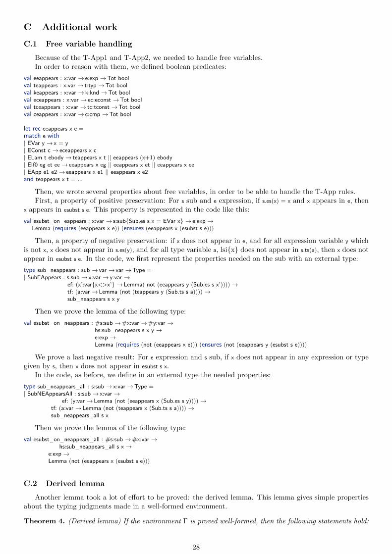
C Additional work

C.1 Free variable handling

Because of the T-App1 and T-App2, we needed to handle free variables.In order to reason with them, we defined boolean predicates:

val eeappears : x:var → e:exp →Tot boolval teappears : x:var → t:typ →Tot boolval keappears : x:var → k:knd →Tot boolval eceappears : x:var → ec:econst →Tot boolval tceappears : x:var → tc:tconst →Tot boolval ceappears : x:var → c:cmp →Tot bool

let rec eeappears x e =match e with| EVar y → x = y| EConst c → eceappears x c| ELam t ebody → teappears x t || eeappears (x+1) ebody| EIf0 eg et ee → eeappears x eg || eeappears x et || eeappears x ee| EApp e1 e2 → eeappears x e1 || eeappears x e2and teappears x t = ...

Then, we wrote several properties about free variables, in order to be able to handle the T-App rules.First, a property of positive preservation: For s sub and e expression, if s.es(x) = x and x appears in e, then

x appears in esubst s e. This property is represented in the code like this:

val esubst on eappears : x:var → s:sub{Sub.es s x = EVar x} → e:exp →Lemma (requires (eeappears x e)) (ensures (eeappears x (esubst s e)))

Then, a property of negative preservation: if x does not appear in e, and for all expression variable y whichis not x, x does not appear in s.es(y), and for all type variable a, lsi{x} does not appear in s.ts(a), then x does notappear in esubst s e. In the code, we first represent the properties needed on the sub with an external type:

type sub neappears : sub → var → var →Type =| SubEAppears : s:sub → x:var → y:var →

ef: (x’:var{x<>x’} → Lemma( not (eeappears y (Sub.es s x’)))) →tf: (a:var → Lemma (not (teappears y (Sub.ts s a)))) →sub neappears s x y

Then we prove the lemma of the following type:

val esubst on neappears : #s:sub →#x:var →#y:var →hs:sub neappears s x y →e:exp →Lemma (requires (not (eeappears x e))) (ensures (not (eeappears y (esubst s e))))

We prove a last negative result: For e expression and s sub, if x does not appear in any expression or typegiven by s, then x does not appear in esubst s x.

In the code, as before, we define in an external type the needed properties:

type sub neappears all : s:sub → x:var →Type =| SubNEAppearsAll : s:sub → x:var →

ef: (y:var → Lemma (not (eeappears x (Sub.es s y)))) →tf: (a:var → Lemma (not (teappears x (Sub.ts s a)))) →sub neappears all s x

Then we prove the lemma of the following type:

val esubst on neappears all : #s:sub →#x:var →hs:sub neappears all s x →

e:exp →Lemma (not (eeappears x (esubst s e)))

C.2 Derived lemma

Another lemma took a lot of effort to be proved: the derived lemma. This lemma gives simple propertiesabout the typing judgments made in a well-formed environment.

Theorem 4. (Derived lemma) If the environment Γ is proved well-formed, then the following statements hold:

28

• Typing judgment: for e expression and M t wp computation, if Γ ` e : M t wp, then Γ ` t : Type

• Kinding judgment: for t type and k kind, if Γ ` t : k, then Γ ` k kwf

• Subtyping judgment: for t’, t types, if Γ ` t’ <: t, then Γ ` t’ : Type and Γ ` t : Type

• Subkinding judgment: for k’, k kinds, if Γ ` k’ <: k, then Γ ` k’ kwf and Γ ` k kwf

• Validity judgment: for phi formula, if Γ |= phi, then Γ ` phi : Type

Just like the substitution lemma, this lemma was proved using an induction on all the judgments. Duringthe proof, we also discovered some bugs in the metatheory.

C.3 Mechanized proof for the weakest-preconditions calculus

At the beginning of my internship, when I was in Saarbrucken to learn how to use F*, I made a projectwith another student, Enrico Steffinlongo.

The goal of this project was to write a mechanized proof of the correctness and completeness of the weakest-precondition calculus on a small language in F*. The correctness part is about proving that the computedprecondition is sufficient to get the postcondition after the execution of the program. The completeness part isabout proving that the computed precondition is the weakest, compared to the other valid Hoare triples withthe same postcondition.

Definitions In order to do this, we first defined the formulas and the deduction system on it:

type form =| FFalse : form| FImpl : form → form → form| FAnd : form → form → form| FForall : (heap →Tot form) → form| FEq : #a:Type → a → a → form

type deduce : form →Type =| DFalseElim :

f:form →deduce FFalse →deduce f

| DImplIntro :f1:form →f2:form →(deduce f1 →Tot (deduce f2)) → (∗ <- meta level implication ∗)deduce (FImpl f1 f2)

| DImplElim :f1:form →

f2:form →deduce (FImpl f1 f2) →deduce f1 →deduce f2

| DAndIntro :f1:form →f2:form →deduce f1 →deduce f2 →deduce (FAnd f1 f2)

...

Then we defined a small language in F*, with its operational semantics:

type com =| Skip : com| Assign : var:id → term:aexp → com| Seq : first:com → second:com → com| If : cond:bexp → then branch:com → else branch:com → com| While : cond:bexp → body:com → inv:pred → com

type reval : com →heap →heap →Type =| ESkip : h0:heap →

reval Skip h0 h0

| EAssign : h0:heap → x:id → e:aexp →

29

reval (Assign x e) h0 (update h0 x (eval aexp h0 e))

| ESeq : #h0:heap →#c1:com →#c2:com →#h1:heap →#h2:heap →reval c1 h0 h1 →reval c2 h1 h2 →reval (Seq c1 c2) h0 h2

| EIfTrue : #h0:heap → be:bexp{eval bexp h0 be = true} →ct:com → ce:com →#h1:heap →reval ct h0 h1 →reval (If be ct ce) h0 h1

| EIfFalse : #h0:heap → be:bexp{eval bexp h0 be = false} →ct:com → ce:com →#h1:heap →reval ce h0 h1 →reval (If be ct ce) h0 h1

| EWhileEnd : #h0:heap → be:bexp{eval bexp h0 be = false} →cb:com → i:pred →reval (While be cb i) h0 h0

| EWhileLoop : #h0:heap → be:bexp{eval bexp h0 be = true} →cb:com → i:pred →#h1:heap →#h2:heap →reval cb h0 h1 →reval (While be cb i) h1 h2 →reval (While be cb i) h0 h2

We then defined what we call Hoare triple in two different ways: one semantically and one syntactically.The semantic definition:

type hoare (p:pred) (c:com) (q:pred) : Type =(#h:heap →#h’:heap → reval c h h’ → deduce (p h) →Tot (deduce (q h’)))

Here, a Hoare triple {p}c{q} is seen as a function which, for any heaps h,h’, takes as argument a reductionproof of the program c which changes the state from h to h’, and the validity of the predicate p on h andproduces the validity of q on h’.

The syntactic definition:

type hoare syn : pred → com → pred →Type =| HoareSynAssign : q:pred → x:id → e:aexp →

hoare syn (pred sub x e q) (Assign x e) q| HoareSynConsequence : p:pred → p’:pred → q:pred → q’:pred → c:com →

hoare syn p’ c q’ →deduce (pred impl p p’) →deduce (pred impl q’ q) →hoare syn p c q

| HoareSynSkip : p:pred →hoare syn p Skip p

| HoareSynSeq : p:pred → c1:com → q:pred → c2:com → r:pred →hoare syn p c1 q →hoare syn q c2 r →hoare syn p (Seq c1 c2) r

| HoareSynIf : p:pred → q:pred → be:bexp → t:com → e:com →hoare syn (pand p (bpred be)) t q →hoare syn (pand p (pnot (bpred be))) e q →hoare syn p (If be t e) q

| HoareSynWhile : p:pred → be:bexp → c:com →hoare syn (pand p (bpred be)) c p →hoare syn p (While be c p) (pand p (pnot (bpred be)))

We finally defined the weakest-precondition calculus:

val wlp : com → pred →Tot predlet rec wlp c q =match c with| Skip → q| Assign x e → pred sub x e q| Seq c1 c2 →wlp c1 (wlp c2 q)| If be ct ce → pif (bpred be) (wlp ct q) (wlp ce q)| While be c’ i →

pand i (fun →FForall (pimpl i (pif (bpred be) (wlp c’ i) q)))

30

ResultsFor the semantic version, we were able to prove only correctness. The completeness part is false with the

semantic definition anyway, because of the while loops. Indeed, the weakest-precondition calculus uses theinvariant given by the loop to build the precondition. But this invariant might not be the most efficient one,and can introduce non-necessary conditions.

The proof of correctness is done by defining a function of the following type:

val wlp sound : c:com → q:pred →Tot (hoare (wlp c q) c q)

For the syntactic version, we were able to prove completeness, by defining a function of the following type:

val wlp weakest’ : c:com → p:pred → q:pred →hpcq:hoare syn p c q →Tot (deduce (pred impl p (wlp c q)))

In the conclusion, (pred impl p (wlp c q)) is the formula which states that the precondition wlp c q is weakerthan p. So the conclusion states precisely what we want. []

References

[1] F*’s home page. https://fstar-lang.org/.

[2] Thorsten Altenkirch and Bernhard Reus. Monadic presentations of lambda terms using generalized in-ductive types. In Computer Science Logic, pages 453–468. Springer, 1999.

[3] Brian E Aydemir, Aaron Bohannon, Matthew Fairbairn, J Nathan Foster, Benjamin C Pierce, PeterSewell, Dimitrios Vytiniotis, Geoffrey Washburn, Stephanie Weirich, and Steve Zdancewic. Mechanizedmetatheory for the masses: The POPLmark challenge. In Theorem Proving in Higher Order Logics, pages50–65. Springer, 2005.

[4] Bruno Barras. Coq en Coq. 1996.

[5] Chris Casinghino, Vilhelm Sjoberg, and Stephanie Weirich. Combining proofs and programs in a depen-dently typed language. ACM SIGPLAN Notices, 49(1):33–45, 2014.

[6] Edsger W Dijkstra. Guarded commands, nondeterminacy and formal derivation of programs. Communi-cations of the ACM, 18(8):453–457, 1975.

[7] C. Keller. Substitutions for simply-typed λ-calculus. Internship Report, Ecole Normale Superieure deLyon, 2008.

[8] C. Keller. The category of simply typed λ-terms in Agda. Unpublished note, 2008.

[9] Aleksandar Nanevski, Greg Morrisett, and Lars Birkedal. Hoare type theory, polymorphism and separa-tion. Journal of Functional Programming, 18(5-6):865–911, 2008.

[10] Steven Schafer, Tobias Tebbi, and Gert Smolka. Autosubst: Reasoning with de bruijn terms and parallelsubstitutions. In Xingyuan Zhang and Christian Urban, editors, Interactive Theorem Proving - 6th Inter-national Conference, ITP 2015, Nanjing, China, August 24-27, 2015, LNAI. Springer-Verlag, Aug 2015.To appear.

[11] Pierre-Yves Strub, Nikhil Swamy, Cedric Fournet, and Juan Chen. Self-certification: bootstrapping cer-tified typecheckers in F* with Coq. In Proceedings of the 39th ACM SIGPLAN-SIGACT Symposium onPrinciples of Programming Languages, POPL 2012, Philadelphia, Pennsylvania, USA, January 22-28,2012, pages 571–584, 2012.

[12] Nikhil Swamy, Juan Chen, Cedric Fournet, Pierre-Yves Strub, Karthikeyan Bhargavan, and Jean Yang.Secure distributed programming with value-dependent types. J. Funct. Program., 23(4):402–451, 2013.

[13] Nikhil Swamy, Catalin Hritcu, Chantal Keller, Aseem Rastogi, Antoine Delignat-Lavaud, Simon Forest,Karthikeyan Bhargavan, Cedric Fournet, Pierre-Yves Strub, Markulf Kohlweiss, and Jean-Karim Zinzin-dohoue. Dependent types and multi-monadic effects in F?. 2016. https://www.fstar-lang.org/papers/mumon/.

31

[14] Nikhil Swamy, Joel Weinberger, Cole Schlesinger, Juan Chen, and Benjamin Livshits. Verifying higher-order programs with the dijkstra monad. In ACM SIGPLAN Notices, volume 48, pages 387–398. ACM,2013.

32