moving from static to dynamic general equilibrium …paltsev/docs/move.pdf · equilibrium model...
TRANSCRIPT

Moving from Static to Dynamic General EquilibriumEconomic Models (Notes for a beginner in MPSGE)
Sergey V. Paltsev ∗
Department of Economics, University of Colorado †
Draft:‡
June 1999 (Revised: June 2000)
Abstract
The document is intended to serve as a guide for beginners in MPSGE. It starts witha short introduction to the class of economic problems which can be solved with MPSGE,followed by a detailed description of step-by-step transformation of a simple static generalequilibrium model into a dynamic Ramsey model. The model is based on a simplified dataset.Two cases are considered: the first dataset represents an economy on the steady-state growthpath and the second dataset is off the steady-state growth path in a base year. The paperincludes GAMS-MPSGE codes which can be copied and used as a starting point for furtherexploration of dynamic economic modelling.
∗Thanks to Thomas Rutherford and Miles Light for not letting me sink when I hit the MPSGE iceberg. Theauthor can be reached at: [email protected]†University of Colorado, Department of Economics, Boulder, CO 80309-0256, USA.‡The latest version of this document in PDF format can be downloaded from
http://debreu.colorado.edu/papers/move.pdf

From Static to Dynamic Models 2
1 Instead of Introduction
“This is not a paper. These are notes for your own understanding” - Thomas Rutherford, theauthor of MPSGE, put these words on the first draft of this document. “I already have a paper ona Ramsey model. Read it.” - he added1. At that time I was (and still am) a poor graduate studentin desperate need for a research assistantship money. So I haven’t told him that I have read hispaper several times. Even after that, my understanding of what MPSGE is and how to build adynamic model was not much better than my understanding of how to build a bridge in Nepal.Therefore, I put these notes together as a reference for myself. Then I thought that if these noteswere helpful for me, they might be useful for other beginners. Tom’s resolution sent the paperto the bottom drawer of my desk for a long time. It was sitting there until the moment whensome people suddenly decided that I know something and asked me the question: “How do youbuild a dynamic model in MPSGE?”. Obviously, my advice for them was to read the Rutherford’spaper. For some reason, which is still unknown to me, almost all of them returned and asked forsomething more clear and detailed. My subsequent explanations in the mix of English and Russianleft them even more confused. At that moment, I decided that the idea that these are “notes forunderstanding” may not be that bad after all. In short, if you are smart as Tom Rutherford, thesenotes are not for you. However, if you have overrated yourself a little bit and still have somequestions about modelling dynamics in MPSGE, you may try to find the answers here. Tom doesnot like to write papers at the beginner’s level. I hope I am stupid enough to try it. Ready? Thenlet’s go through the basics together.
In the next section, I will try to share my understanding of what is MPSGE and what kindof problems can be solved with its help. Section 3 describes how a simple static model can berepresented in the MPSGE format. If you are already familiar with MPSGE, you may skip thatpart and turn directly to section 4, which shows the transition of a static model into a dynamicmodel2. This is done for the case where an economy is initially on a steady-state growth path.Section 5 presents adjustments in the model, which are necessary for the off steady-state case.Program listings are provided in the Appendices. I have also included Appendices on MPSGE-MCP conversion and representation of different functional forms in MPSGE format. They are notdirectly relevant to dynamic models. However, they are important for better understanding theprocess of economic modelling with MPSGE.
Finally, I am always amazed by those IMF and The World Bank-like disclaimers. Now I alsohave a chance to provide one. Here it is: “The views expressed in this document are those ofthe author and do not necessarily reflect the views of the MPSGE creator.” In simple English itmeans that these notes are just notes for my own understanding. If you have any questions aboutMPSGE, then “ask Tom”.
2 MPSGE and General Economic Equilibrium Models
MPSGE (Mathematical Programming System for General Equilibrium Analysis) is a programminglanguage designed by Thomas Rutherford [1999] in late 80s for solving Arrow-Debreu economicequilibrium models. The MPSGE is very powerful but badly documented language. Due to thatfact, the usual recipe for mastering in MPSGE is “learning by doing”.
MPSGE uses the programming language GAMS (General Algebraic Modeling System) as aninterface3. As a result, if one wants to use MPSGE, he needs to learn basic GAMS syntax4 (Brook,Kendrick, Meeraus [1992]) as well. As it follows from the name, MPSGE solves computable general
1I refer to this dynamic modelling paper (Lau, Pahlke, Rutherford [1997]) as the Rutherford’s paper. It isavailable at: http://nash.colorado.edu/tomruth/primer/paper.htm
2The discussion in this paper is limited to a Ramsey model. Another approach to introducing dynamics isoverlapping generations (OLG) models. For OLG formulation in MPSGE, see Rutherford [1998].
3To learn more about GAMS, visit their homepage at http://www.gams.com4As of April 2000, a free student version of GAMS is available at: http://www.gams.de/5download/cd.htm
From Static to Dynamic Models 3
equilibrium (CGE) economic models. These models consist of economic agents who interact amongeach other. The word “general” means that all economic flows are accounted for, i.e there is a“sink” for every “source”. Finding an equilibrium for a CGE model involves finding equilibriumprices, quantities, and incomes.
As an illustration of a simple economic model, consider the task of finding an equilibrium inthe economy (for the future reference I will call it Wonderland), which consists of two economicagents: consumers and producers. Consumers have an initial endowment of labor L and capitalK. For simplicity, there is a single representative consumer5 CONS in Wonderland. The consumerderives his income I from the sales of his endowments. Then he purchases his preferred choiceof goods. There are two goods, X and Y , in the economy. The consumer obtains utility fromconsumption of the goods. Producers are the firms that take initial endowments of the consumeras inputs of production and convert them into outputs. Both production sectors, X and Y , arecharacterized by the available technology F and G, respectively.
We want to determine the prices and quantities which maximize producers’ profits and con-sumer’s utility6. The solution to this problem (which is a simple Arrow-Debreu [1954] problem)can be found using a non-linear formulation. It can be represented as an optimization problem ofthe consumer subject to income, technology, and feasibility constraints.
maxW (X,Y ) s.t I = pxX + pyYX = F (Kx, Lx)Y = G(Ky, Ly)L = Lx + LyK = Kx +Ky
where W is a utility function, px and py are the prices of goods X and Y , Kx and Lx are capitaland labor used in the production sector X, Ky and Ly are capital and labor used in the sectorY . This is a standard microeconomic textbook optimization problem, and a usual technique forfinding the solution is the method of Lagrange multipliers. This problem can be solved in GAMSas a non-linear programming (NLP).
There are some cases (such as a presence of several consumers, taxes, or other distortions)where it is not possible to solve the problem of finding a market equilibrium as an optimizationproblem. Then the problem could be approached in a different way. It can be turned into a MixedComplimentarity Problem (MCP) and solved as a system of non-linear equations. NLP problemsare a subset of MCP and MPSGE finds an equilibrium as a solution to MCP.
Here is the first test to check if you should be reading these notes or go directly to Ruther-ford’s [1997] paper. I had never heard about MCP formulation before. When I asked about it, aknowledgeable person told me that it is very easy, something like:
Given: f : Rn → Rn
Find: z ∈ Rns.t. f(z) ≥ 0, z ≥ 0, zT f(z) = 0.
If everything is clear for you in the statement above, you are wasting your time with these notes.Close them and go to do real work!
If you are still here, then let’s try to convert the mathematical symbols into simple English. Ishould tell that it won’t help very much to a beginner because it sounds like: given the functionf between two n-dimensional sets of real numbers (function f assigns to each member of the firstset exactly one member of the second set), find z which belongs to an n-dimensional set of realnumbers, such that function f (z) is greater or equal to zero, z is greater or equal to zero, and
5Or, equivalently, a population of identical households.6It sounds funny for non-economists that there is a single consumer who owns the firms and purchases the
goods produced by these firms. But for economists with their “economic way of thinking” it seems natural. Thesignificance of this assumption is that distributional considerations between different types of consumers are ignored.

From Static to Dynamic Models 4
associated complimentary slackness condition7 is satisfied. The complimentary slackness conditionrequires that either z equals zero (i.e. the dual multiplier vanishes), or the inequality constraint issatisfied with strict equality, or both.
However, these words is just a usual scientific way of hiding something simple. Do you recallfrom your 6th grade math the solution to an equation like: x(5 − x) = 0? Yes, it is x = 0 andx = 5. To make it more clear for a comparison, the equation above can be rewritten as xf(x) = 0,where f(x) = 5 − x. It leads to the condition that either x or f(x) has to be equal zero. This isthe main idea behind MCP.
In the case when we have not just one x, but a vector of x̄ = (x1, x2, ..., xn), then there is asystem of n equations like x̄f(x̄) = 0, which forms an MCP problem. The word “mixed” in MCPreflects the fact that the solution is a mix of equalities f(x) = 0 and inequalities f(x) > 0.
Mathiesen [1985] has shown that the Arrow-Debreu economic equilibrium model can be formu-lated as MCP, where three inequalities should be satisfied: zero profit condition, market clearancecondition, and income balance condition. A set of three non-negative variables is involved in solv-ing MCP problem: prices, quantities (they are called as activity levels in MPSGE), and incomelevels.
Zero profit condition requires that any activity operated at a positive intensity must earn zeroprofit (i.e. value of inputs must be equal or greater than value of outputs). Activity levels y forconstant returns to scale production sectors are the associated variables with this condition. Itmeans that either y > 0 (a positive amount of y is produced) and profit is zero, or profit isnegative and y = 0 (no production activity takes place). In terms of MCP, the following conditionshould be satisfied for every sector in an economy:
−profit ≥ 0, y ≥ 0, outputT (−profit) = 0
Market clearance condition requires that any good with positive price must have a balancebetween supply and demand and any good in excess supply must have a zero price. Price vector p(which includes prices of final goods, intermediate goods and factors of production) is associatedvariable. In terms of MCP, the following condition should be satisfied for every good and everyfactor of production:
supply − demand ≥ 0, p ≥ 0, pT (supply − demand) = 0
Income balance condition requires that for each agent (including any government entities) valueof income must equal the value of factor endowments. Is it possible to formulate it in terms ofMCP:
(endowment− income) ≥ 0, income ≥ 0, incomeT (endowment− income) = 0
However, income usually does not equal to zero and the condition endowment − income = 0 issatisfied as an equality. As such, income balance condition is definitional rather than complimen-tary.
To illustrate the equilibrium conditions, consider the Wonderland example. For the reasonswhich will be clear later, additional production sector W is introduced to represent utility derivedfrom the consumption of X and Y . Accordingly, Pw is a price of the output of the productionsector W . First, consider zero profit conditions. In the Wonderland example, an activity level yis a vector with the following components y = (X,Y,W ). Profit in a particular sector is definedas a difference between total revenue and total cost. We assume that activity levels X, Y , and Ware positive (i.e., the condition y ≥ 0 is satisfied with the strict inequality as y > 0). Hence, zeroprofit conditions ((−profit) = 0) can be written as
−(Px − Cx(w, r)) = 0, (1)
7An expression written as xT y = 0 means xiyi = 0, for all i = 1, ..., n. The variables xi and yi are called acomplementary pair and are said to be complements to each other
From Static to Dynamic Models 5
−(Py − Cy(w, r)) = 0, (2)
−(Pw − e(Px, Py)) = 0, (3)
where Cx, Cy are unit cost functions for X and Y (cost of production of one unit of a good underthe factor prices w and r); e is a unit cost (expenditure) function for W (cost of buying one unitof utility under the prices Px and Py).
Market clearance condition requires that if prices are positive then supply should be equal todemand. It is represented by the following equations
X =∂e
∂PxW, (4)
Y =∂e
∂PyW, (5)
W =I
Pw, (6)
L =∂Cx∂w
X +∂Cy∂w
Y, (7)
K =∂Cx∂r
X +∂Cy∂r
Y. (8)
On the demand side, partial derivatives ∂e/∂Pi, ∂Ci/∂w, and ∂Ci/∂r represent Shephard’s lemma8.Income balance condition states that the value of endowments equals consumer’s income:
wL+ rK = I (9)
MPSGE would solve nine equations (1-9) for nine unknowns: activity levels, X,Y,W ; prices,Px, Py, Pw, w, r; and income I. It should be noted that equilibrium conditions are hard to formulatein an explicit form for certain problems. The good news for a MPSGE user is that one doesnot need to spend any time deriving the equilibrium conditions. MPSGE builds them for youautomatically. However, it is always helpful to understand what the algebraic representation ofa particular MPSGE model is9. For a comparison, alternative formulations of a simple model oftaxation and international trade (Shoven and Whalley [1984]) in MPSGE and its algebraic form(MCP formulation) are presented in Appendix 2. An MCP formulation of a dynamic Ramseyproblem can be found in the Rutherford’s paper. In order to run MPSGE program, MCP solversshould be used. GAMS has two MCP solvers: MILES and PATH. In Tom’s words, MILES is hisabandoned child, which leaves PATH as the first choice.
3 A Static Model
In the previous section we have briefly discussed how MPSGE finds an equilibrium. It is niceto know that MPSGE will solve it not as an optimization problem, but instead by finding anequilibrium in a system of inequalities. However, in order to create a simple MPSGE programa user does not need to know this. What is much more important for a beginner is the syntaxof the MPSGE language10. A big advantage of MPSGE is that it is based on nested constantelasticity of substitution (CES) utility and production functions11. Use of nested functions can
8For more information on Shephard’s lemma see, for example, Varian [1992].9When I saw an MPSGE code for the first time, I said: “I need to see an underlying algebra”. Later on I have
realized that MPSGE representation is much more attractive and intuitive than its algebraic formulation. So nowthe knowledgeable person always smiles when I am saying: “I don’t want those ugly MCP equations, show me anMPSGE code”.
10MPSGE syntax can be found at http://debreu.colorado.edu/mainpage/mpsge.htm11See Appendix 1 for the examples of conversion of different functions into the MPSGE format.

From Static to Dynamic Models 6
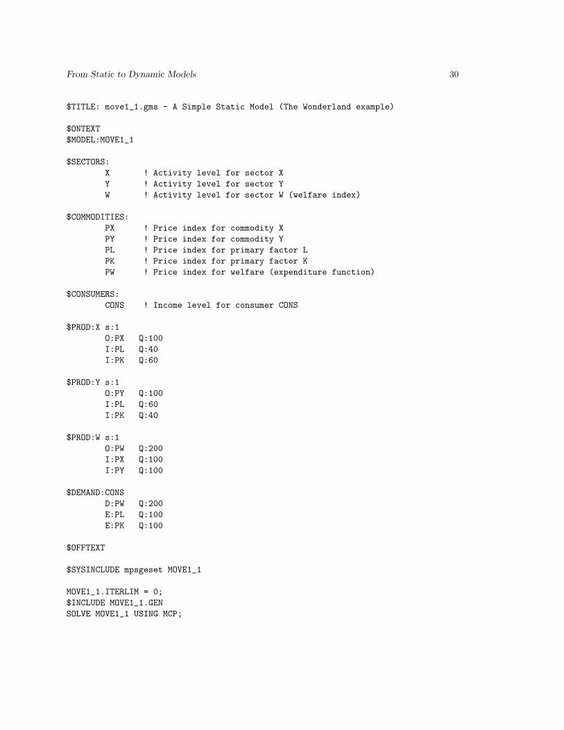
provide a flexible representation of how inputs are related. To introduce the MPSGE syntax12, wewill consider again the Wonderland example described in Section 2. The GAMS-MPSGE programof the Wonderland static model (move1 1.gms) is listed in Appendix 3.
Economic models are based on data which in turn are usually organized into a Social Ac-counting Matrix (SAM)13. We assume the following data represented in Table 1 where a SAM hasthree production sectors X, Y, and W (they are declared in the $SECTORS block of the MPSGEprogram), one consumer CONS (declared in the $CONSUMERS block), and five markets X, Y, W,L, and K (declared in the $COMMODITIES block). Because the variables which are associated withcommodities are their prices, they usually begin with the letter P.
Production Sectors ConsumersMarkets X Y W CONS
PX 100 -100PY 100 -100PW 200 -200PL -40 -60 100PK -60 -40 100
Table 1. A Static Model SAM (the Wonderland example)
A SAM describes a data set, which is usually referred to as a benchmark dataset. Numbersrepresent the values (price times quantity) of economic transactions in a given period of time. Apositive entry means a value of output (or sales). A negative entry reflects a value of input (orpurchases). Zero profit, market clearance and income balance conditions imply that row sums andcolumn sums are equal to zero.
To illustrate how SAM is balanced, consider the following row and column of Table 1. Aproduction sector X purchases 40 units14 of labor and 60 units of capital, and sales 100 units ofgood X . The sum over X column is equal to zero. It shows that there is no excess profit (zeroprofit) in the sector X. A row PX shows that 100 units of X which are produced and sold (positiveentry of 100) are consumed by sector W (negative entry of 100). The sum over PX row is equal tozero. It shows that supply equals to demand (market clearance) for a good X.
For simplicity, sometimes a Harberger convention is adopted in a benchmark SAM. It consistsin normalizing all prices to 1. Then quantities in a SAM represent expenditures, or how much of agood or factor one can buy for $1. It should be noted that an Arrow-Debreu economy only dependupon relative prices. Doubling all prices double money profits and income, which is resulted inthe same solution for quantities (or activity levels). The absolute price level has no impact on theequilibrium outcome.
As it has already been noted, MPSGE does not require a user to formulate an algebraic repre-sentation of production and utility functions. The user only needs to provide reference quantities,reference prices, and elasticities. Based on provided information, MPSGE constructs underly-ing production and utility functions. At the solution, MPSGE returns equilibrium values for thevariables, described in $SECTORS, $COMMODITIES, and $CONSUMERS.
In the Wonderland example, there are two products (X and Y), two factors (L and K), and oneconsumer (CONS). An extra row and column (PW and W) are introduced in order to explicitlyrepresent utility derived from an aggregate consumption. As we will discuss later, it could havebeen done directly in the $DEMAND block15.
12In this treatment of simple static and dynamic models, many MPSGE features are not going to be dis-cussed. For additional practice, see the Markusen examples (Markusen and Rutherford [1995]), available at:http://nash.colorado.edu/tomruth/6433/markusen.htm .
13For more information on converting input-output data into an MPSGE model, see Rutherford and Paltsev [1999]14Make sure to remember that units here represent the value, i.e. price times quantity.15However, a separate block for utility is helpful for an introduction of a consumption tax and for welfare analysis.

From Static to Dynamic Models 7
The program starts with declaration of the title, which will be printed in a solution listing.Usually, GAMS-formatted declarations of scalars, parameters, and sets then follow. We do notneed them in our simple static model. The next portion is in MPSGE format.
$ONTEXT$MODEL:NAMEThese two blocks shifts control from GAMS to MPSGE compiler. Model name is chosen by a user.For example, our model has the name MOVE1 1. The model name has to be a legitimate filename,because a file NAME.GEN (MOVE1 1.GEN in our case) is going to be generated.
$SECTORS:In this block, production sectors are declared. They determine how inputs are converted intooutputs. The variables here are activity levels and they are associated with zero profit conditions(i.e. they make sure that a production sector earn zero profit). In the Wonderland model, we havethree sectors: X, Y, and W. Comments can be made in the same line after ! mark.
$COMMODITIES:Commodities are declared in this block. The variables here are prices. They are associated withmarket clearance conditions (i.e. they make sure that supply is equal to demand). We have fivecommodities: two output prices PX, PY, two factor prices PK, PL, and price index PW for welfare(i.e. utility derived from an aggregate consumption).
$CONSUMERS:Consumers who supply factors and receive utility are described. The variable here is income fromall sources. It is associated with income balance condition (i.e. it makes sure that total income isequal to total consumption (or total demand)). In our case, we have one representative consumerCONS.
$PROD:Production block constructs the underlying production function (i.e., the rule how inputs areconverted into output). Sectors and commodities used in a production block should be declared inrespective blocks. Consider the first production block for X (Production blocks for Y and W havea similar structure):
$PROD:X s:1O:PX Q:100I:PL Q:40I:PK Q:60
This block describes a Cobb-Douglas production function (we can see it from s:1, which meansthat the elasticity of substitution between inputs is equal to one). Inputs here are PL and PK(we can see it from I:PL and I:PK). Output is PX (O:PX). This production sector converts 40units of PL and 60 units of PK into 100 units of PX. Mathematically, the production function forthis technology can be written as X = φL0.4 K0.6 (See Appendix 1 for conversion of productionand utility function into the MPSGE format). Figure 1 illustrates the calibration of a productionfunction to benchmark prices and quantities.

From Static to Dynamic Models 8
K
60
L40
isoquant X=100 (s:1)
@@@@@@@@@@@@
isocost (slope = -1)
Fig.1. Production function calibration
MPSGE specifies the production function with a single reference point. In this example wehave explicitly specified reference quantities only. Reference prices are set to 1 by default. Relativeprice of inputs determines the slope of isocost (which in turn equals to the slope of isoquant at thereference quantities). It means that our production block is identical to:
$PROD:X s:1O:PX Q:100 P:1I:PL Q:40 P:1I:PK Q:60 P:1
The curvature of isoquant is determined by s, the elasticity of substitution between inputs (s : 1corresponds to a Cobb-Douglas production function). Default value for elasticity is zero. Thereference quantities and prices are used only for calibration. They are not used by the solver asstarting values of the variables. Production block Y is similar to X.
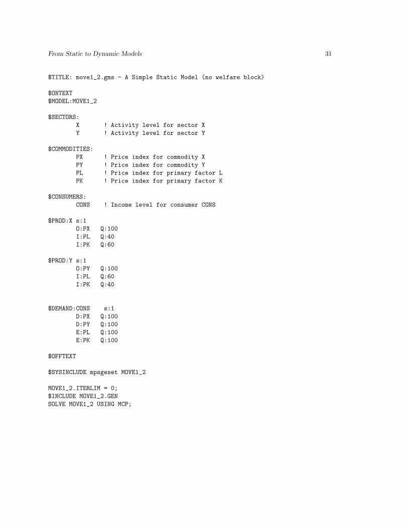
Production block for W (Welfare) serves as a tool for conversion of goods X and Y consumptioninto utility derived from an aggregate consumption. In this simple model we have introduced thisproduction block for clarity purposes only. We could have eliminated the production block W andchanged the demand block into16
$DEMAND:CONSD:PX Q:100D:PY Q:100E:PL Q:100E:PK Q:100
However, in more complicated models the representation of welfare as a production block may bevery useful (for example, in the analysis of a consumption tax).
$DEMAND:Demand block represents an income balance constraint.
16See the code of the program move1 2.gms from Appendix 3. You can run it to compare the results withmove1 1.gms.

From Static to Dynamic Models 9
$DEMAND:CONSD:PW Q:200E:PL Q:100E:PK Q:100
A consumer receives income from its L and K endowments (E:PK and E:PL) and demands goodPW (D:PW). Reference quantities (Q fields) are used for calibration of the utility function in thesame way that the production block calibrates production function.
$OFFTEXT$SYSINCLUDE mpsgeset NAMEThese two blocks shift control from MPSGE back to GAMS.
NAME.ITERLIM = 0;This command determines the number of iterations. With zero iteration limit, we tell the solvernot to solve the model but to return the values which are based on the initial data. Setting theiteration limit to zero is important to assure that the benchmark data (i.e., the data described ina SAM) represent the equilibrium solution.
$INCLUDE NAME.GENSOLVE NAME USING MCP;These two blocks are used for running the model.
The solution of the static model (reported in a listing (move1 1.lst) file) is:
LOWER LEVEL UPPER MARGINAL
VAR X . 1.0000 +INF .VAR Y . 1.0000 +INF .VAR W . 1.0000 +INF .VAR PX . 1.0000 +INF .VAR PY . 1.0000 +INF .VAR PL . 1.0000 +INF .VAR PK . 1.0000 +INF .VAR PW . 1.0000 +INF .VAR CONS . 200.0000 +INF .
In the solution, LOWER and UPPER columns show the bounds of respective variables. Zerois represented by “.”. INF means infinity. The LEVEL column reports the solution value. TheMARGINAL column shows the value of the complimentary slackness (shadow) variable. We needto pay close attention to LEVEL and MARGINAL columns. Complimentary slackness implies thatin equilibrium, either the level of a variable will be positive or the marginal value will be positive,but not both. If both of them are positive, we need to check our model.
The solution to the static model tells us that the benchmark data (represented in the SAM)are consistent with the equilibrium of the model. We can see it because all marginals are equalto zero after benchmark replication (i.e., after solving the model with ITERLIM=0). Equilibriumactivity levels X, Y, and Z are equal to 1 (and not to 100, 100, and 200 as in SAM !). Equilibriumprices are equal to 1. Equilibrium income level of a representative consumer is equal to 200.
Somewhat confusing for beginners is that activity levels in the solution are all equal to one.This is just due to rescaling and it is done for the purpose of future analysis of counterfactualexperiments, where a user can easily see the percentage change of a value deviated from 1. If wewant to see unscaled activity levels, we need to multiply the levels from the solution by Q: fieldsin the production blocks. For example, for the activity level X it equals to 1*100=100.
From Static to Dynamic Models 10
There are other ways to get actual activity levels in the solution listing. One possible way isto rescale production blocks and assign initial values for activities as it is done in the programmove1 3.gms. The solution for this case directly replicates the benchmark data:
LOWER LEVEL UPPER MARGINAL
VAR X . 100.0000 +INF .VAR Y . 100.0000 +INF .VAR W . 200.0000 +INF .VAR PX . 1.0000 +INF .VAR PY . 1.0000 +INF .VAR PL . 1.0000 +INF .VAR PK . 1.0000 +INF .VAR PW . 1.0000 +INF .VAR CONS . 200.0000 +INF .
However, for numerical reasons, it is advisable to scale equilibrium values close to unity. That iswhy it is better to use a REPORT block as it is shown in the program move1 4.gms, where theinitial SAM is recreated using the reported values.
All initial values for activity levels and prices are equal to 1 by default. A variable CONS,which represents a consumer income level, is somewhat different. It is determined by endowments.Remember from income balance condition that income is equal to total value of endowments, andin turn equal to total demand. In the case of static model it is equal to 200 because endowment ofcapital (E:PK) is 100 and endowment of labor (E:PL) is 100, and prices PK and PL are equal to1 by default.
As we have noted, the model determines only relative prices. So if we assign all initial pricesas being equal to 2, then variable CONS will be calculated to be equal to 400. We can check itby modifying the static model. Initial price levels can be assigned after $SYSINCLUDE mpsgesetNAME, but before $INCLUDE NAME.GEN command in the following way:
PX.L = 2;PY.L = 2;PW.L = 2;PK.L = 2;PL.L = 2;
Then the solution listing shows an increase in all prices and the income level.
LOWER LEVEL UPPER MARGINAL
VAR X . 1.0000 +INF .VAR Y . 1.0000 +INF .VAR W . 1.0000 +INF .VAR PX . 2.0000 +INF .VAR PY . 2.0000 +INF .VAR PL . 2.0000 +INF .VAR PK . 2.0000 +INF .VAR PW . 2.0000 +INF .VAR CONS . 400.0000 +INF .
Due to determination of relative prices only, usually one price is fixed by a user. If no price is fixedinitially (i.e. no good is chosen as a numeraire), then MPSGE will do a default price normalization.In the case of our static model, a consumer’s income level CONS is fixed. It can be seen in thesolution listing file (.lst) by looking at the statement Default price normalization usingincome for CONS.

From Static to Dynamic Models 11
The model can also be specified in a different format. Instead of using numbers in referencequantity and price field, we could have introduced parameters at the beginning of the programand used them for calibration in the fields of production and demand blocks. An example of thevector syntax is presented in the program move1 5.gms.
After benchmark calibration, counterfactual experiments (for example, an introduction oftaxes or changes in labor endowment) are performed. It is important to remember to changethe iteration limit before running counterfactuals, which is done with the GAMS statement likeNAME.ITERLIM=2000;. The solver will stop as soon as this limit is reached if the solution is notfound before a user defined number of iterations. In this paper, we will not describe any counter-factuals with our static model17. Our interest here is different and consists of the conversion ofthe static model into a dynamic one.
4 Dynamic models
When I had started to learn economic modeling, I immediately wanted to build a dynamic model.I wanted to predict the future, so what kind of predictions one can make with a static model?Later on, I realized that my attempts of dynamic modeling were like a desire to build a spaceshipwith a screwdriver only. Besides, I wanted too much out of dynamic models. Dynamic models arenowhere near the goal of predicting the future. A model can more or less tell you what is goingto happen if there are no shocks and structural changes in an economy. In addition, one need tomake assumptions about the rate of economic growth for several decades into the future, the rateof time preference, the growth rate of population, inflation, depreciation, etc. All these necessaryassumptions bring us very far from the reality. But policy makers still need to make their decisionsand economists need to provide answers about the future. Therefore, dynamic general equilibriummodels are important tools for economic policy evaluation. But now I know that it is much moreinformative to develop a good static model than a poor dynamic one (and so far, I have never everseen a good dynamic model).
With such an encouragement, we will attempt to develop a dynamic model based on the Won-derland example. There are different approaches to dynamic economic modeling (see, Ginsburghand Keyzer [1997] for an overview). We limit our discussion to a simple Ramsey model. The modelbehaves differently if it is on a so called steady-state than it is not. A steady-state is defined asa situation in which the various quantities (such as capital, output, consumption, etc.) grow atconstant rates. We start our consideration with the situation when benchmark data describe aneconomy on a steady-state in a base period.
4.1 An economy on a steady-state in a base period
In a dynamic version of the Wonderland example, a representative consumer maximizes the presentvalue of his lifetime utility
max∞∑t=0
(1
1 + ρ
)tU(ct), (10)
where t - time periods, ρ - individual time-preference parameter, U - utility function, ct - con-sumption in period t. The consumer faces several constraints. First, total output produced in theeconomy is divided to consumption and investment, It. Second, capital depreciates at the rate δ.Third, investment cannot be negative. This constraints can be written as
ct ≤ F (Kt, Lt)− It, (11)
17See Markusen examples for practice (Markusen and Rutherford [1995]).
From Static to Dynamic Models 12
Kt+1 = Kt(1− δ) + It, (12)
It ≥ 0, (13)
where K is capital and F represents production function. Solving the utility maximization problemresults in the following first-order conditions:
Pt = (1
1 + ρ)t∂U(ct)∂ct
, (14)
PKt = (1− δ)PKt+1 + Pt∂F (Kt, Lt)
∂Kt, (15)
Pt = PKt+1, (16)
where Pt, PKt, and PKt+1 are the values of the corresponding Lagrange multipliers. They canbe interpreted as the price of output, the price of capital today, and the price of capital tomorrow,respectively. The utility maximization problem above is formulated as an NLP problem. As hasalready been discussed, MPSGE solves it as an MCP problem. Let RKt and Wt represent rentalrate of capital and wage rate in period t. Denote unit cost function
as C(RKt,Wt) and demand functionas D(Pt,M), where M is consumer’s income. Then MCP can be formulated as follows.Zero profit conditions:
Pt ≥ PKt+1, It ≥ 0, It(Pt − PKt+1) = 0 (17)
PKt ≥ RKt + (1− δ)PKt+1, Kt ≥ 0, Kt(PKt −RKt + (1− δ)PKt+1) = 0 (18)
C(RKt,Wt) ≥ Pt, Yt ≥ 0, Yt(C(RKt,Wt)− Pt) = 0 (19)
Market clearance conditions:
Yt ≥ D(Pt,M) + It, Pt ≥ 0, Pt(Yt −D(Pt,M) + It) = 0 (20)
Lt ≥ Yt∂C(RKt,Wt)
∂Wt, Wt ≥ 0, Wt(Lt − Yt
∂C(RKt,Wt)∂Wt
) = 0 (21)
Kt ≥ Yt∂C(RKt,Wt)
∂RKt, RKt ≥ 0, RKt(Kt − Yt
∂C(RKt,Wt)∂RKt
= 0 (22)
Income balance condition:
M = PK0K0 +∞∑t=0
WtLt, M > 0 (23)
As noted before, a modeller does not need to program these equilibrium conditions explicitly.MPSGE constructs them automatically. However, we need to describe a change in capital overtime. This requires modification of the SAM, presented in Table 1. We add one more productionsector for investment. This, in turn, will change the composition of the welfare block W, becausenow output can be consumed or invested, rather than just consumed as in the static case.
From Static to Dynamic Models 13
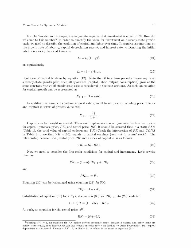
For the Wonderland example, a steady-state requires that investment is equal to 70. How didwe come to this number? In order to quantify the value for investment on a steady-state growthpath, we need to describe the evolution of capital and labor over time. It requires assumptions onthe growth rate of labor, g, capital depreciation rate, δ, and interest rate, r. Denoting the initiallabor force as L0, labor at time t is
Lt = L0(1 + g)t, (24)
or, equivalently,
Lt = (1 + g)Lt−1. (25)
Evolution of capital is given by equation (12). Note that if in a base period an economy is ona steady-state growth path, then all quantities (capital, labor, output, consumption) grow at thesame constant rate g (off steady-state case is considered in the next section). As such, an equationfor capital growth can be represented as
Kt+1 = (1 + g)Kt. (26)
In addition, we assume a constant interest rate r, so all future prices (including price of laborand capital) in terms of present value are:
Pt+1 =Pt
1 + r. (27)
Capital can be bought or rented. Therefore, implementation of dynamics involves two pricesfor capital: purchase price, PK, and rental price, RK. It should be stressed that in a static SAM(Table 1), the total value of capital endowment, V K (Check the intersection of PK and CONSin Table 1 to see that V K =100), equals to capital earnings (and not to capital stock!). Therelationship between V K, rental price RK and a stock of capital K is as follows:
V Kt = Kt ·RKt. (28)
Now we need to consider the first-order conditions for capital and investment. Let’s rewritethem as
PKt = (1− δ)PKt+1 +RKt (29)
and
PKt+1 = Pt. (30)
Equation (30) can be rearranged using equation (27) for PK:
PKt = (1 + r)Pt. (31)
Substitution of equation (31) for PKt and equation (30) for PKt+1 into (29) leads to:
(1 + r)Pt = (1− δ)Pt +RKt. (32)
As such, an equation for the rental price is18:
RKt = (δ + r)Pt (33)
18Setting P(t) = 1, an equation for RK makes perfect economic sense, because if capital and other loans areperfect substitutes, then households can also receive interest rate r on lending to other households. But capitaldepreciates at the rate δ. Then r = RK − δ, or RK = δ + r, which is the same as equation (33).

From Static to Dynamic Models 14
From equations (12) and (26), we have the following rule for investment on a steady-state
It = (δ + g)Kt, (34)
or using (28) and (33), investment in a base period is equal to
I0 =(δ + g)V K0
δ + r. (35)
Equation (35) describes the value of investment which we need to introduce into the SAM for asteady-state growth path. We assume19 δ = 0.05, g = 0.02, and r = 0.05. Then, investment isI = (0.05 + 0.02) · 100/(0.05 + 0.05) = 70. We assume that goods are invested in the same propor-tion (35:35). In addition, we need to modify the welfare block W by dividing it into consumptionand savings. The total amount of produced goods is 200, 70 of which is invested. It leaves 130units for consumption in a base period, 65 of which is consumption of good X and another 65 isconsumption of good Y. The benchmark SAM after these changes is represented in Table 2.
Production Sectors ConsumersMarkets X Y W inv CONS
PX 100 -65 -35PY 100 -65 -35PW 200 -200PL -40 -60 100PK -60 -40 100sav -70 70
Table 2. Dynamic Model SAM
An important characteristic of the dynamic problem is a treatment of capital in the last periodof modeling. We cannot solve numerically for an infinite number of periods, hence, some adjust-ments are needed for approximation of finite horizon model to the infinite horizon choices. Specialprocedures should be introduced for the terminal capital, otherwise, all capital would be consumedin the last period and nothing would be invested. We have followed the Rutherford’s paper andintroduced the level of post-terminal capital as a variable and added a constraint on the growthrate of investment in the terminal period:
ITIT−1
=YTYT−1
, (36)
where T is a terminal period. The advantage of the usage of this constraint is that it imposesbalanced growth in the terminal period but does not require that the model achieve steady-stategrowth. The meaning of the constraint is that investment in a terminal period should grow at thesame rate as output20.
A program listing of the dynamic model is represented in Appendix 3 (file move2 1.gms). Belowwe list and then discuss the changes which are necessary to make in the code of the static model.
1. Introduce time sets;
2. Declare the assumed interest rate, growth rate and depreciation rate;19It should be noted that the transversality condition requires that r > g, otherwise, there is a possibility of a
chain-letter borrowing (for detailed discussion see, for example, Barro and Sala-i-Martin (1995)).20Because all quantities grow at the same rate, it is possible to use a growth of total output, output in a certain
production sector, or consumption (or simply 1+g in a steady-state case) as a right-hand side variable of equation(36).
From Static to Dynamic Models 15
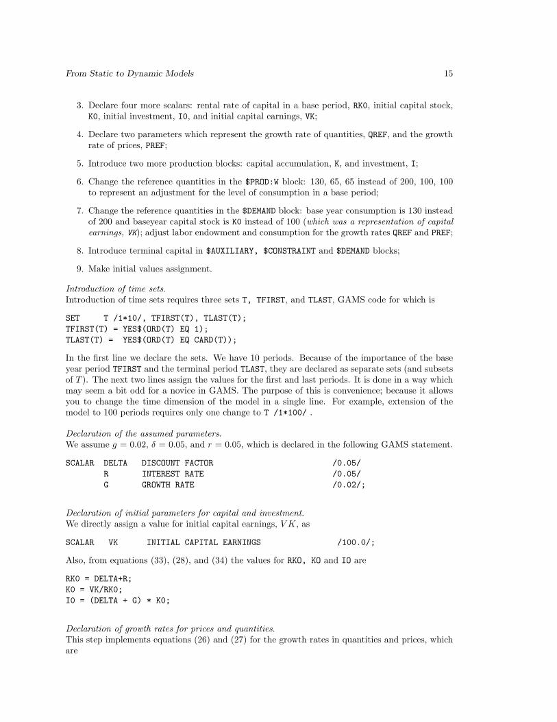
3. Declare four more scalars: rental rate of capital in a base period, RK0, initial capital stock,K0, initial investment, I0, and initial capital earnings, VK;
4. Declare two parameters which represent the growth rate of quantities, QREF, and the growthrate of prices, PREF;
5. Introduce two more production blocks: capital accumulation, K, and investment, I;
6. Change the reference quantities in the $PROD:W block: 130, 65, 65 instead of 200, 100, 100to represent an adjustment for the level of consumption in a base period;
7. Change the reference quantities in the $DEMAND block: base year consumption is 130 insteadof 200 and baseyear capital stock is K0 instead of 100 (which was a representation of capitalearnings, VK); adjust labor endowment and consumption for the growth rates QREF and PREF;
8. Introduce terminal capital in $AUXILIARY, $CONSTRAINT and $DEMAND blocks;
9. Make initial values assignment.
Introduction of time sets.Introduction of time sets requires three sets T, TFIRST, and TLAST, GAMS code for which is
SET T /1*10/, TFIRST(T), TLAST(T);TFIRST(T) = YES$(ORD(T) EQ 1);TLAST(T) = YES$(ORD(T) EQ CARD(T));
In the first line we declare the sets. We have 10 periods. Because of the importance of the baseyear period TFIRST and the terminal period TLAST, they are declared as separate sets (and subsetsof T ). The next two lines assign the values for the first and last periods. It is done in a way whichmay seem a bit odd for a novice in GAMS. The purpose of this is convenience; because it allowsyou to change the time dimension of the model in a single line. For example, extension of themodel to 100 periods requires only one change to T /1*100/ .
Declaration of the assumed parameters.We assume g = 0.02, δ = 0.05, and r = 0.05, which is declared in the following GAMS statement.
SCALAR DELTA DISCOUNT FACTOR /0.05/R INTEREST RATE /0.05/G GROWTH RATE /0.02/;
Declaration of initial parameters for capital and investment.We directly assign a value for initial capital earnings, V K, as
SCALAR VK INITIAL CAPITAL EARNINGS /100.0/;
Also, from equations (33), (28), and (34) the values for RKO, KO and IO are
RK0 = DELTA+R;K0 = VK/RK0;I0 = (DELTA + G) * K0;
Declaration of growth rates for prices and quantities.This step implements equations (26) and (27) for the growth rates in quantities and prices, whichare

From Static to Dynamic Models 16
QREF(T) = (1 + G) ** (ORD(T) - 1);PREF(T) = (1/(1 + R)) ** (ORD(T) - 1);
We have ORD(T)-1 as an exponent to represent the fact that in the base year QREF and PREF areequal to 1 and grow thereafter.
Production blocks for capital and investment.New production block for K(T) implements capital accumulation as it represented by equation(29). The MPSGE format of the production block is (we skip terminal capital for a moment):
$PROD:K(T)O:PK(T+1) Q:(K0*(1-DELTA))O:RK(T) Q:(K0*(R+DELTA))I:PK(T) Q:K0
Those who learn the MPSGE representation of the Ramsey dynamic model are mostly confusedby the reference quantity of RK(T). The difference with equation (29) is that in the productionblock the reference quantity for capital rental price21 is K0*(R+DELTA), whereas in equation (29)(r + δ) does not appear as a coefficient of RKt. The dynamic model would not calibrate withoutthis reference quantity. The reason for this is the fact that RK is used in several production blocks:X, Y , and K and we need to to reflect the relationship between RKt and Pt given by equation(33)
Alternatively, we could have used K0 as a reference price for O:RK(T) and assign the rental pricegrowth as RK.L(T) = (DELTA+R)*PREF(T);, but in this case the input fields for production of Xand Y blocks should also be changed as represented in the program move2 2.gms of Appendix 3.
Production block I introduces equation (30). We assume that investment is split equallybetween two production sectors.
$PROD:I(T) S:0O:PK(T+1) Q:I0I:PY(T) Q:(0.5*I0)I:PX(T) Q:(0.5*I0)
Note that S:0 corresponds to Leontief production function, i.e., elasticity of substitution betweeninputs is equal to zero. If no elasticity is specified in a production block, MPSGE uses zero elasticityas a default value. Therefore, S:0 can be skipped from the code of this block.
Change in the Welfare block.We need to make changes in the production of W , because in the dynamic version of the modelnot all output is consumed but some portion of it is invested. From Table 2 we know the newvalues for output (Q:130) and inputs (Q:65).
Change in the Demand block.For the same reason, in the DEMAND block we need to modify a reference quantity for PW(T)from 200 to 130. Also, growth in consumption and labor over time is represented by QREF(T).
We use the reference price PREF(T) as the value of the discount on the future consumptiongiven by equation (10). Introduction of individual time-preference as a separate parameter is notneeded because in the Ramsey model, the steady-state leads to a constant pattern of per capitaconsumption and to the condition that ρ = r.
Another change in the DEMAND block involves the usage of initial capital stock K0 as areference quantity for PK(TFIRST), instead of the value of capital V K as in the static case. Thisis determined by income balance condition of the dynamic model.
21Note that K0*(R+DELTA)=VK, so we could have used Q:VK as a reference quantity for O:RK(T).
From Static to Dynamic Models 17
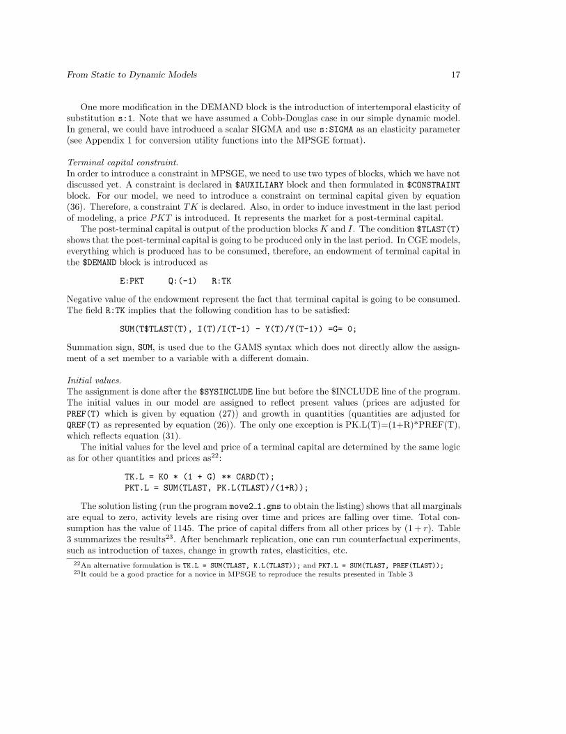
One more modification in the DEMAND block is the introduction of intertemporal elasticity ofsubstitution s:1. Note that we have assumed a Cobb-Douglas case in our simple dynamic model.In general, we could have introduced a scalar SIGMA and use s:SIGMA as an elasticity parameter(see Appendix 1 for conversion utility functions into the MPSGE format).
Terminal capital constraint.In order to introduce a constraint in MPSGE, we need to use two types of blocks, which we have notdiscussed yet. A constraint is declared in $AUXILIARY block and then formulated in $CONSTRAINTblock. For our model, we need to introduce a constraint on terminal capital given by equation(36). Therefore, a constraint TK is declared. Also, in order to induce investment in the last periodof modeling, a price PKT is introduced. It represents the market for a post-terminal capital.
The post-terminal capital is output of the production blocks K and I. The condition $TLAST(T)shows that the post-terminal capital is going to be produced only in the last period. In CGE models,everything which is produced has to be consumed, therefore, an endowment of terminal capital inthe $DEMAND block is introduced as
E:PKT Q:(-1) R:TK
Negative value of the endowment represent the fact that terminal capital is going to be consumed.The field R:TK implies that the following condition has to be satisfied:
SUM(T$TLAST(T), I(T)/I(T-1) - Y(T)/Y(T-1)) =G= 0;
Summation sign, SUM, is used due to the GAMS syntax which does not directly allow the assign-ment of a set member to a variable with a different domain.
Initial values.The assignment is done after the $SYSINCLUDE line but before the $INCLUDE line of the program.The initial values in our model are assigned to reflect present values (prices are adjusted forPREF(T) which is given by equation (27)) and growth in quantities (quantities are adjusted forQREF(T) as represented by equation (26)). The only one exception is PK.L(T)=(1+R)*PREF(T),which reflects equation (31).
The initial values for the level and price of a terminal capital are determined by the same logicas for other quantities and prices as22:
TK.L = K0 * (1 + G) ** CARD(T);PKT.L = SUM(TLAST, PK.L(TLAST)/(1+R));
The solution listing (run the program move2 1.gms to obtain the listing) shows that all marginalsare equal to zero, activity levels are rising over time and prices are falling over time. Total con-sumption has the value of 1145. The price of capital differs from all other prices by (1 + r). Table3 summarizes the results23. After benchmark replication, one can run counterfactual experiments,such as introduction of taxes, change in growth rates, elasticities, etc.
22An alternative formulation is TK.L = SUM(TLAST, K.L(TLAST)); and PKT.L = SUM(TLAST, PREF(TLAST));23It could be a good practice for a novice in MPSGE to reproduce the results presented in Table 3

From Static to Dynamic Models 18
Quantities Prices X Y W K I1 1.0000 1.0000 100.00 100.00 130.00 1000.00 70.002 1.0200 0.9524 102.00 102.00 132.60 1020.00 71.403 1.0404 0.9070 104.04 104.04 135.25 1040.40 72.834 1.0612 0.8638 106.12 106.12 137.96 1061.21 74.295 1.0824 0.8227 108.24 108.24 140.72 1082.43 75.776 1.1041 0.7835 110.41 110.41 143.53 1104.08 77.297 1.1262 0.7462 112.62 112.62 146.40 1126.16 78.838 1.1487 0.7107 114.87 114.87 149.33 1148.69 80.419 1.1717 0.6768 117.17 117.17 152.32 1171.66 82.0210 1.1951 0.6446 119.51 119.51 155.36 1195.09 83.66
Table 3. Steady-state prices and quantities
4.2 Calibrating dynamic models to a benchmark data which are not ona steady-state
Data for a base period may be inconsistent with a steady-state growth path. Table 4 gives anexample of the situation where investment is “too big”, i.e., from equation (35) the value ofinvestment is 80 > (0.05 + 0.02) · 100/(0.05 + 0.05) = 70.
Production Sectors ConsumersMarkets X Y W Inv CONS
PX 100 -60 -40PY 100 -60 -40PW 200 -200PL -40 -60 100PK -60 -40 100sav -80 80
Table 4. A Dynamic Model SAM off a Steady-State
One possible solution for model calibration in the case of the off-steady-state data is to assumethat g is the labor growth rate, but the capital growth rate is different initially and converges to gover time24. We use the calibration which is based on the secant algorithm. It finds the solutionto an equation f(x) = 0 as:1. Initial guess on x(n), where n is the number of iteration.2. Calculate x(n+ 1) as25:
xn+1 = xn −f(xn)
f(xn)− f(xn−1)(xn − xn−1) (37)
To reiterate our current dynamic problem, we know the initial values given in the SAM. TheSAM is not consistent with a steady-state growth path. Also, we know (assumed) depreciation rateand long-run interest rate but the rental price in a base period is unknown. Our goal is calibratinga dynamic model to the data represented in the SAM. In order to do that we use iterations basedon the secant algorithm described above. The calibration involves the following iteration process:
24Another way of calibrating to a static data set involves given data on a base year investment, interest rate, andreturn to capital. The long-run steady-state interest rate is determined based on assumed labor growth rate andcalibrated utility discount rate.
25Equation (37) could be derived from an equation of tangent: y−ynx−xn
= f ′(xn). Put y = 0 and yn = f(xn), then
x = xn − f(xn)f ′(xn)) . Using f ′(xn) = f(xn)−f(xn−1)
xn−xn−1we receive equation (37).

From Static to Dynamic Models 19
guessing initial rental rate of capital, RK0, calculating a model of the transition path, observinginvestment, I0, in the current equilibrium, and adjusting RK0.
The program listing for the off-steady-state dynamic model is provided in Appendix 3 (filemove3 1.gms). At first, we guess about the rental price, RKG, in the first period. In the on-steady-state case the rental price (which is also equal to return to capital) is δ + r. We make our guessusing this knowledge. Note that if our guess is “too far”, the algorithm does not work. Also, ifinvestment is “too far” from the steady-state value, the algorithm does not work as well.
The off-steady-state dynamic program has the same structure as before, except for the factthat we have used an alternative formulation similar to the program described in Appendix 3 (filemove2 2.gms). We apply equation (37) for finding f(x), which is in our case the difference betweenthe value of investment calculated in the program and the one given in the SAM. Accordingly, x(n)is the guess on rental price at the first period. During the first iteration we simply add 0.1 to ourguess value for RK0 in order to produce a basis for further iterations. During all other iterationswe reproduce equation (37) as
RKG = RKG + ERROR(ITER)/(ERROR(ITER-1)-ERROR(ITER))* (RK0VAL(ITER)-RK0VAL(ITER-1));
where ERROR represents26 f(x) and RK0VAL represents x(n).The last portion of the program includes graphing the results for investment, consumption,
growth rate and interest rate. We have used GNUPLOT utility to produce graphs. It can beseen from the graphs (run the model move3 1.gms to obtain the graphs) that the values eventuallyconverge to a steady-state growth path. The speed of convergence to a steady-state is determinedby production and preference parameters (Barro and Sala-i-Martin [1995]).
4.3 Dynamic GTAP
Adjustments similar to the described above can be applied to a static model of the GTAPinGAMSpackage (Rutherford [1998b]). The listing of the dynamic model is presented in Appendix 4.
5 Conclusion
Learn MPSGE!!!
References
[1] Arrow, K.J., and G. Debreu (1954). “Existence of an Equilibrium for a Competitive Economy.”Econometrica, 22, 265-90.
[2] Barro, R.J., and X. Sala-i-Martin (1995). Economic Growth, McGraw-Hill.
[3] Brooke, A., D. Kendrick, and A. Meeraus (1992). GAMS: A User’s Guide, Release 2.25,Scientific Press.
[4] Ginsburgh V., and M. Keyzer (1997). The Structure of Applied General Equilibrium Models,The MIT Press.
[5] Lau M.I., A. Pahlke, and T.F. Rutherford (1997). “Modeling Economic Adjustment: A Primerin Dynamic General Equilibrium Analysis”, University of Colorado. Working Paper, availableat: http://nash.colorado.edu/tomruth/primer/paper.htm
26Note that for f(x) we use an equation for consumption instead of investment in order to explicitly separatecalculated and given values. Usage of ERROR(ITER) = I.L("1")*I0 - I0; instead of ERROR(ITER) = C.L("1") -(200-I0); produces the same result.

From Static to Dynamic Models 20
[6] Markusen, J.R., and T.F. Rutherford (1995). The Markusen examples. Notes for GAMSworkshop, 1995. (available athttp://nash.colorado.edu/tomruth/6433/markusen.htm)
[7] Mathiesen, L. (1985). “Computation of Economic Equilibrium by a Sequence of Linear Com-plementarity Problems”, Mathematical Programming Study 23, North-Holland, pp. 144-162.
[8] Rutherford, T.F. (1998). “Overlapping Generations with Pure Exchange: An MPSGE For-mulation”, University of Colorado, mimeo, available at: http://debreu.colorado.edu/ tom-ruth/olg/exchange/index.html
[9] Rutherford, T.F. (1998b). “GTAPinGAMS: The Dataset and Static Model”, University of Col-orado, available at: http://debreu.colorado.edu/ tomruth/gtapingams/html/gtapgams.html
[10] Rutherford, T.F. (1999). “Applied General Equilibrium Modeling with MPSGE as a GAMSSubsystem: An overview of the Modeling Framework and Syntax”, Computational Economics,V.14, Nos. 1-2.
[11] Rutherford, T.F., and S.V. Paltsev (1999). From an Input-Output Table to a General Equi-librium Model: Assessing the Excess Burden of Indirect Taxes in Russia. University of Col-orado. Working Paper. (available at http://nash.colorado.edu/gams-x/ruswebfiles/gams-cgi-stat.html)
[12] Varian, H.R. (1992). Microeconomic Analysis, Third Edition, Norton & Company.

From Static to Dynamic Models 21
Appendix 1. Conversion of production and utility functionsinto the MPSGE format
MPSGE represents production and preferences as nested CES functions.
Production:A production technology is identically represented by either the production function or corre-sponding cost function. A general form of a nested CES production function is X(K,L) =(aKρ + (1 − a)Lρ)
1ρ where ρ is the substitution parameter (−∞ < ρ < 1), which is related to
the elasticity of substitution σ as σ = 11−ρ . When ρ = −∞ (or σ = 0), CES production function
converts into Leontief (or fixed proportions) production function X1(K,L) = min(aK1, (1−a)L1).When ρ = 1 (or σ =∞), then inputs are perfect substitutes in production X2 = aK2 + (1− a)L2.When ρ = 0 (or σ = 1), then CES production function converts into a Cobb-Douglas caseX3(K,L) = Ka
3 L1−a3 .
Let’s consider MPSGE representation of a particular example of a Cobb-Douglas productionfunction: X(K,L) = K0.6L0.4. The following production blocks represent the same technology:a)
$PROD:X s:1O:PX Q:1I:PK Q:0.6I:PL Q:0.4
b)
$PROD:X s:1O:PX Q:100I:PK Q:60I:PL Q:40
c)
$PROD:X s:1O:PX Q:100I:PK Q:60 P:2I:PL Q:40 P:2
d)
$PROD:X s:1O:PX Q:100 P:2I:PK Q:60I:PL Q:40
e)
$PROD:X s:1O:PX Q:100 P:2I:PK Q:60 P:2I:PL Q:40 P:2

From Static to Dynamic Models 22
Remember that reference prices and quantities are used for calibration only and not transferred toa solver as initial values! Another important issue is that only relative prices matter. As such, useof P:1 or P:2 for both inputs gives the same marginal rate of substitution. Price of output doesnot matter in this example because we have one output only. In the case of two outputs relativeprices would matter as they determine marginal rate of transformation.
How about this production block?
$PROD:X s:1O:PX Q:1I:PK Q:1 P:0.6I:PL Q:1 P:0.4
It still represents the same production technology (?) as all above MPSGE production blocks.Now consider a production block:
$PROD:X s:1O:PX Q:1I:PK Q:0.6 P:2I:PL Q:0.4
This production block is described by the function X(K,L) = K0.75L0.25, because value sharesare: K = 0.6
1.2+0.4 = 0.75 and L = 0.41.2+0.4 = 0.25.
Leontief production function can be represented either as
$PROD:X s:0O:PX Q:100I:PK Q:60I:PL Q:40
or as
$PROD:XO:PX Q:100I:PK Q:60I:PL Q:40
because default value for top level elasticity is zero.
Preferences:
General form of a nested CES utility function is U(X,Y ) = (aXρ + (1 − a)Y ρ)1ρ where ρ is
an elasticity parameter. Elasticity of substitution σ is related to elasticity parameter as σ = 11−ρ .
$DEMAND block represents utility derived from consumption of goods and consumer’s endowments.If quantities demanded and endowments are all equal to 100, then demand block in MPSGE is:
$DEMAND:CONS s:(1/1-RHO)D:PX Q:100D:PY Q:100E:PL Q:100E:PK Q:100
There is a particular utility function which is widely used in a dynamic analysis. It is aConstant Intertemporal Elasticity of Substitution utility function (CIES), which has a form:
U(Ct) = C1−θt −11−θ , where σ = 1
θ is the elasticity of substitution.As θ → 0, U(C) approaches a linear case U(Ct) = Ct−1 (which represent the same preferences
as U(Ct) = Ct). As θ → 1, then U(Ct) = ln(Ct).

From Static to Dynamic Models 23
In order to see a relationship between CES and CIES utility functions, we start with CESform: U(Ct) = (aCρt )
1ρ . Then substitute ρ = 1 − θ because σ = 1
θ and σ = 11−ρ . It leads
to U(C) = (aC1−θ)1
1−θ . Maximization of (aC1−θ)1
1−θ and aC1−θ
1−θ produces the same result foroptimal value of C (because maxX
1b ⇔ maxXb ⇔ max X
b ). For utility maximization overinfinite horizon we sum over instanteneous utilities and adjust for a discount factor, which leadsto a traditional form of utility function:
U =∑∞t=0( 1
1+ρ )t C1−θt −11−θ .
If a consumer has an endowment of labor and capital and elasticity of intertemporal substitutionSIGMA between consumption in different periods is defined as SIGMA=1/THETA; to reflect therelationship between σ and θ, then $DEMAND block for CIES utility function has the following form:
$DEMAND:CONS s:SIGMAD:PC(T) Q:QREF(T) P:PREF(T)E:PL(T) Q:QREF(T)E:PK(TFIRST) Q:K0
Note that if consumer gets utility from two goods (for example, in a Cobb-Douglas form) wecan keep the same $DEMAND block as above and add a production block
$PROD:C(T) s:1O:PC(T) Q:C0I:PX(T) Q:X0I:PY(T) Q:Y0
Multilevel nestsConsider a case when T=1,2. Then from production block
a)
$PROD:C s:1O:PC Q:C0I:PX(T) Q:X0I:PY(T) Q:Y0
elasticity between PX1, PX2, PY1, PY2 is 1.b)
$PROD:C s:1 a:0.5O:PC Q:C0I:PX(T) Q:X0 a:I:PY(T) Q:Y0
elasticity between PX1 and PX2 is 0.5, and elasticity between PY1, PY2 and PX1:PX2 is 1.c)
$PROD:C s:1 a:0.5 b:1.5O:PC Q:C0I:PX(T) Q:X0 a:I:PY(T) Q:Y0 b:
elasticity between PX1 and PX2 is 0.5, elasticity between PY1 and PY2 is 1.5, and elasticitybetween PX1:PX2 and PY1:PY2 is 1.
d)
$PROD:C s:1 a:0.5O:PC Q:C0I:PX(T) Q:X0 a:I:PY(T) Q:Y0 a:
From Static to Dynamic Models 24
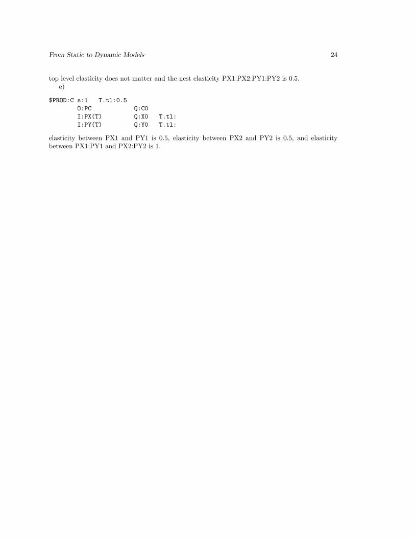
top level elasticity does not matter and the nest elasticity PX1:PX2:PY1:PY2 is 0.5.e)
$PROD:C s:1 T.tl:0.5O:PC Q:C0I:PX(T) Q:X0 T.tl:I:PY(T) Q:Y0 T.tl:
elasticity between PX1 and PY1 is 0.5, elasticity between PX2 and PY2 is 0.5, and elasticitybetween PX1:PY1 and PX2:PY2 is 1.

From Static to Dynamic Models 25
Appendix 2. MPSGE and algebraic formulation
Appendix 2 contains the MPSGE and algebraic (MCP) versions for the following problem (Shovenand Whalley, Applied General-Equilibrium Models of Taxation and International Trade: An Intro-duction and Survey, Journal of Economic Literature, Vol. 22, No. 3. (Sep., 1984), pp. 1007-1051).It is provided for illustration purposes. One can compare the degree of difficulty in both versions.If you are interested in an MCP version of a dynamic Ramsey model, see Rutherford’s [1997] pa-per. I have some preliminary notes on conversion of MPSGE into MCP. Check with me if I havefinished them yet.
In this model, there are two final commodities (M, N), two factors of production (K, L) and twoconsumers (R,P). Producers are competitive, minimizing unit cost taking market prices as given.Production functions are of the constant-elasticity-of-substitution (CES) form:
Qi = φi [δiLρii + (1− δ)Kρi
i ]1/ρi i ∈M,N
where ρi = (σi−1)/σi, and σi is an elasticity of substitution between capital and labor. Parametersof the production function are given by:
Sector φi δi σiManufacturing (M) 1.5 0.6 2.0
Non-Manufacturing (N) 2.0 0.7 0.5
Consumers are endowed with primary factors form which they earn income. This income is usedto purchase goods to maximize utility. The CES utility functions are:
Uc =
[∑i
α1/σcic Xρc
ic
]1/ρc
c ∈ R,P
where ρc = (σc−1)/σc, and σc is an elasticity of substitution between goods M and N. Commodityendowments and parameters of the utility function are given by:
Household K L αM αN σcRich 25 0 0.5 0.5 1.5Poor 0 60 0.3 0.7 0.75
After computing the benchmark equilibrium, a single counterfactual experiment is done inwhich a 50% ad-valorem tax is levied on each unit of capital services employed in the manufacturingsector. Tax revenue is returned as lump-sum income for the two households, 40% to the rich and60% to the poor.
$title Compare MPSGE and its algebraic representation
set i /M, N/;set c /RICH, POOR/;set rich(c) /rich/;set poor(c) /poor/;
parameterssigma /m 2, n 0.5/,phi /m 1.5, n 2/,delta /m 0.6, n 0.7/,sig /rich 1.5, poor 0.75/,capital /rich 25, poor 0/,labor /rich 0, poor 60/;

From Static to Dynamic Models 26
table alpha(c,i)M N
RICH 0.5 0.5POOR 0.3 0.7 ;
parameter taxrate(i);
$ontext$model:work
$SECTORS:Y(i) !Production
$COMMODITIES:P(i) !PriceW !Price of laborR !Price of capital
$CONSUMERS:cons(c) ! Representative agent
$prod:y(i) s:sigma(i)o:p(i) q:phi(i)i:w q:1 p:delta(i)i:r q:1 p:(1-delta(i))
+ a:cons("rich") t:(0.4*taxrate(i))+ a:cons("poor") t:(0.6*taxrate(i))
$demand:cons(c) s:sig(c)d:p(i) q:1 p:(alpha(c,i)**(1/sig(c)))e:r q:capital(c)e:w q:labor(c)
$offtext$sysinclude mpsgeset work
taxrate(i) = 0;work.iterlim = 5000;$include work.gensolve work using mcp;
taxrate("M") = 0.5;$include work.gensolve work using mcp;
* MCP version
alias(i,j);
taxrate("M") = 0;

From Static to Dynamic Models 27
parameter pk0(i);pk0(i) = 1+taxrate(i);
parameter thetak(i), thetal(i);thetak(i) = 1-delta(i);thetal(i) = delta(i);
parameter abeta(c,i);abeta(c,i) = alpha(c,i)**(1/sig(c));
equationsprf_y(i)mkt_y(i)mkt_kmkt_li_cons(c);
* Zero profit
prf_y(i)..(thetak(i)*(r*(1+taxrate(i))/(pk0(i)*(1-delta(i))))**(1-sigma(i))+ thetal(i)*(w/delta(i))**(1-sigma(i)))**(1/(1-sigma(i)))=e= p(i) * phi(i);
* Market clearance
mkt_y(i)..y(i) * phi(i) =e=sum(c, 1 *((((sum(j, abeta(c,j) * (p(j)/abeta(c,j))** (1-sig(c))))**(1/(1-sig(c)))) * abeta(c,i) / p(i)) ** sig(c)) *cons(c) / ( ((sum(j, abeta(c,j) * (p(j)/abeta(c,j))** (1-sig(c))))**(1/(1-sig(c))))) );
mkt_k..sum(c, capital(c)) =e=sum(i,((thetal(i)*(w/delta(i))**(1-sigma(i))+ thetak(i)*(r*(1+taxrate(i))/(pk0(i)*(1-delta(i))))**(1-sigma(i)))**(1/(1-sigma(i))) / (r*(1+taxrate(i))/(pk0(i)*(1-delta(i)))))**(sigma(i)) * y(i));
mkt_l..sum(c, labor(c)) =e=sum(i,((thetal(i)*(w/delta(i))**(1-sigma(i))+ thetak(i)*(r*(1+taxrate(i))/(pk0(i)*(1-delta(i))))**(1-sigma(i)))**(1/(1-sigma(i))) * delta(i)/w)**(sigma(i)) * y(i));
i_cons(c)..cons(c) =e= r*capital(c) + w*labor(c)
From Static to Dynamic Models 28
+ (sum(i, 0.6 * taxrate(i) * y(i) * r *((thetal(i)*(w/delta(i))**(1-sigma(i))+ thetak(i)*(r*(1+taxrate(i))/(pk0(i)*(1-delta(i))))**(1-sigma(i)))**(1/(1-sigma(i)))/ (r*(1+taxrate(i))/(pk0(i)*(1-delta(i)))))**(sigma(i))))$poor(c)+ (sum(i, 0.4 * taxrate(i) * y(i) * r *((thetal(i)*(w/delta(i))**(1-sigma(i))+ thetak(i)*(r*(1+taxrate(i))/(pk0(i)*(1-delta(i))))**(1-sigma(i)))**(1/(1-sigma(i)))/ (r*(1+taxrate(i))/(pk0(i)*(1-delta(i)))))**(sigma(i))))$rich(c);
model obana /prf_y.y, mkt_y.p, mkt_k.r, mkt_l.w, i_cons.cons/;
cons.fx("rich") = 34.3368;cons.fx("poor") = 60.0000;obana.iterlim = 5000;solve obana using mcp;
* Introduce tax
taxrate("M") = 0.5;cons.fx("rich") = 29.0935;cons.fx("poor") = 61.3484;solve obana using mcp;

From Static to Dynamic Models 29
Appendix 3. Program listings
Appendix 3 contains GAMS programs which can be copied and executed. The following files arelocated here.
move1 1.gms Static model The Wonderland examplemove1 2.gms no welfare blockmove1 3.gms initial quantities in the listingmove1 4.gms report blockmove1 5.gms vector syntaxmove2 1.gms Dynamic model on a steady-state in a baseyearmove2 2.gms alternative formulation of capital blockmove3 1.gms not on a steady-state in a baseyear
From Static to Dynamic Models 30
$TITLE: move1_1.gms - A Simple Static Model (The Wonderland example)
$ONTEXT$MODEL:MOVE1_1
$SECTORS:X ! Activity level for sector XY ! Activity level for sector YW ! Activity level for sector W (welfare index)
$COMMODITIES:PX ! Price index for commodity XPY ! Price index for commodity YPL ! Price index for primary factor LPK ! Price index for primary factor KPW ! Price index for welfare (expenditure function)
$CONSUMERS:CONS ! Income level for consumer CONS
$PROD:X s:1O:PX Q:100I:PL Q:40I:PK Q:60
$PROD:Y s:1O:PY Q:100I:PL Q:60I:PK Q:40
$PROD:W s:1O:PW Q:200I:PX Q:100I:PY Q:100
$DEMAND:CONSD:PW Q:200E:PL Q:100E:PK Q:100
$OFFTEXT
$SYSINCLUDE mpsgeset MOVE1_1
MOVE1_1.ITERLIM = 0;$INCLUDE MOVE1_1.GENSOLVE MOVE1_1 USING MCP;
From Static to Dynamic Models 31
$TITLE: move1_2.gms - A Simple Static Model (no welfare block)
$ONTEXT$MODEL:MOVE1_2
$SECTORS:X ! Activity level for sector XY ! Activity level for sector Y
$COMMODITIES:PX ! Price index for commodity XPY ! Price index for commodity YPL ! Price index for primary factor LPK ! Price index for primary factor K
$CONSUMERS:CONS ! Income level for consumer CONS
$PROD:X s:1O:PX Q:100I:PL Q:40I:PK Q:60
$PROD:Y s:1O:PY Q:100I:PL Q:60I:PK Q:40
$DEMAND:CONS s:1D:PX Q:100D:PY Q:100E:PL Q:100E:PK Q:100
$OFFTEXT
$SYSINCLUDE mpsgeset MOVE1_2
MOVE1_2.ITERLIM = 0;$INCLUDE MOVE1_2.GENSOLVE MOVE1_2 USING MCP;

From Static to Dynamic Models 32
$TITLE: move1_3.gms. Simple Static Model: Formulation for Initial Quantities
$ONTEXT$MODEL:MOVE1_3
$SECTORS:X ! Activity level for sector XY ! Activity level for sector YW ! Activity level for sector W (welfare index)
$COMMODITIES:PX ! Price index for commodity XPY ! Price index for commodity YPL ! Price index for primary factor LPK ! Price index for primary factor KPW ! Price index for welfare (expenditure function)
$CONSUMERS:CONS ! Income level for consumer CONS
$PROD:X s:1O:PX Q:1I:PL Q:0.4I:PK Q:0.6
$PROD:Y s:1O:PY Q:1I:PL Q:0.6I:PK Q:0.4
$PROD:W s:1O:PW Q:1I:PX Q:0.5I:PY Q:0.5
$DEMAND:CONSD:PW Q:200E:PL Q:100E:PK Q:100
$OFFTEXT
$SYSINCLUDE mpsgeset MOVE1_3
X.L=100;Y.L=100;W.L=200;
MOVE1_3.ITERLIM = 0;$INCLUDE MOVE1_3.GENSOLVE MOVE1_3 USING MCP;

From Static to Dynamic Models 33
$TITLE: move1_4.gms - A Simple Static Model (report block)
$ONTEXT$MODEL:MOVE1_4
$SECTORS:X ! Activity level for sector XY ! Activity level for sector YW ! Activity level for sector W (welfare index)
$COMMODITIES:PX ! Price index for commodity XPY ! Price index for commodity YPL ! Price index for primary factor LPK ! Price index for primary factor KPW ! Price index for welfare (expenditure function)
$CONSUMERS:CONS ! Income level for consumer CONS
$PROD:X s:1O:PX Q:100I:PL Q:40I:PK Q:60
$PROD:Y s:1O:PY Q:100I:PL Q:60I:PK Q:40
$PROD:W s:1O:PW Q:200I:PX Q:100I:PY Q:100
$DEMAND:CONSD:PW Q:200E:PL Q:100E:PK Q:100
$REPORT:V:X_OUT O:PX PROD:XV:K_X I:PK PROD:XV:L_X I:PL PROD:XV:Y_OUT O:PY PROD:YV:K_Y I:PK PROD:YV:L_Y I:PL PROD:YV:W_OUT O:PW PROD:WV:X_W I:PX PROD:WV:Y_W I:PY PROD:WV:C D:PW DEMAND:CONS

From Static to Dynamic Models 34
$OFFTEXT
$SYSINCLUDE mpsgeset MOVE1_4
MOVE1_4.ITERLIM = 0;$INCLUDE MOVE1_4.GENSOLVE MOVE1_4 USING MCP;
parameter report;
report("px","X") = x_out.l;report("py","y") = y_out.l;report("pw","w") = w_out.l;report("pl","X") = -l_x.l;report("pk","X") = -k_x.l;report("pl","y") = -l_y.l;report("pk","y") = -k_y.l;report("px","w") = -x_w.l;report("py","w") = -y_w.l;report("pl","cons") = l_x.l+l_y.l;report("pk","cons") = k_x.l+k_y.l;report("pw","cons") = -w_out.l;
display report;

From Static to Dynamic Models 35
$TITLE: move1_5.gms - A Simple Static Model (vector syntax)
set i Sectors /x,y/,f Factors /k,l/;
TABLE sam(*,*) Benchmark data
X Y W CONSX 100 -100Y 100 -100W 200 -200L -40 -60 100K -60 -40 100 ;
PARAMETER Y0(I) Benchmark sectoral output,FD0(F,I) Benchmark factor demands,C0(I) Benchmark consumption demand,E0(F) Factor endowments,W0 Benchmark total consumption;
* Extract data from the original format into model-specific arrays:
Y0(I) = SAM(I,I);FD0(F,I) = -SAM(F,I);C0(I) = -SAM(I,"W");W0 = SUM(I, C0(I));E0(F) = SAM(F,"CONS");
$ONTEXT$MODEL:MOVE1_5
$SECTORS:OUT(i) ! Production Activity LevelW ! Welfare Index
$COMMODITIES:P(i) ! Price index for commoditiesPF(f) ! Price index for factorsPW ! Utility Price Index
$CONSUMERS:CONS ! Income level for consumer CONS
$PROD:OUT(i)O:P(i) Q:Y0(i)I:PF(f) Q:FD0(f,i)
$PROD:W s:1

From Static to Dynamic Models 36
O:PW Q:W0I:P(i) Q:C0(i)
$DEMAND:CONSD:PW Q:W0E:PF(f) Q:E0(f)
$REPORT:V:OUT_o(i) O:P(i) PROD:OUT(i)V:INP(f,i) I:PF(f) PROD:OUT(i)V:OUT_w O:PW PROD:WV:INP_w(i) I:P(i) PROD:WV:C D:PW DEMAND:CONS
$OFFTEXT
$SYSINCLUDE mpsgeset MOVE1_5
MOVE1_5.ITERLIM = 0;$INCLUDE MOVE1_5.GENSOLVE MOVE1_5 USING MCP;
parameter report;
report(i,i) = out_o.l(i);report("w","w") = out_w.l;report(i,"w") = -inp_w.l(i);report(f,i) = inp.l(f,i);report(f,"cons") = sum(i, inp.l(f,i));report("w","cons") = -out_w.l;
display report;

From Static to Dynamic Models 37
$TITLE: move2_1.gms. A Simple Ramsey Dynamic Model
SET T /1*10/,TFIRST(T),TLAST(T);
TFIRST(T) = YES$(ORD(T) EQ 1);TLAST(T) = YES$(ORD(T) EQ CARD(T));
SCALAR DELTA DISCOUNT FACTOR /0.05/R INTEREST RATE /0.05/G GROWTH RATE /0.02/VK INITIAL CAPITAL EARNINGS /100.0/K0 INITIAL CAPITAL STOCKRK0 INITIAL RETURN TO CAPITALI0 INITIAL INVESTMENT;
PARAMETER QREF(T) QUANTITIESPREF(T) PRICES;
RK0 = DELTA+R;K0 = VK/RK0;I0 = (DELTA + G) * K0;QREF(T) = (1 + G) ** (ORD(T) - 1);PREF(T) = (1/(1 + R)) ** (ORD(T) - 1);
$ONTEXT$MODEL:MOVE2_1
$SECTORS:X(T) ! Activity level for sector XY(T) ! Activity level for sector YW(T) ! Activity level for sector W (welfare index)I(T) ! Investment SectorK(T) ! Capital Accumulation
$COMMODITIES:PX(T) ! Price index for commodity XPY(T) ! Price index for commodity YPL(T) ! Price index for primary factor LPK(T) ! Price index for primary factor KPW(T) ! Price index for welfare (expenditure function)RK(T) ! Rental rate for capitalPKT ! Post-terminal capital constraint
$CONSUMERS:CONS ! Income level for consumer CONS
$AUXILIARY:TK ! Terminal Capital Stock

From Static to Dynamic Models 38
$PROD:X(T) s:1O:PX(T) Q:100I:PL(T) Q:40I:RK(T) Q:60
$PROD:Y(T) s:1O:PY(T) Q:100I:PL(T) Q:60I:RK(T) Q:40
$PROD:K(T)O:PK(T+1) Q:((1-DELTA)*K0)O:PKT$TLAST(T) Q:((1-DELTA)*K0)O:RK(T) Q:(K0*(DELTA+R))I:PK(T) Q:K0
$PROD:I(T)O:PK(T+1) Q:I0O:PKT$TLAST(T) Q:I0I:PY(T) Q:(0.5*I0)I:PX(T) Q:(0.5*I0)
$PROD:W(T) s:1O:PW(T) Q:130I:PX(T) Q:65I:PY(T) Q:65
$DEMAND:CONS s:1D:PW(T) Q:(130*QREF(T)) P:PREF(T)E:PL(T) Q:(100*QREF(T))E:PK(TFIRST) Q:K0E:PKT Q:(-1) R:TK
$CONSTRAINT:TKSUM(T$TLAST(T), I(T)/I(T-1) - Y(T)/Y(T-1)) =G= 0;
$OFFTEXT
$SYSINCLUDE mpsgeset MOVE2_1
X.L(T) = QREF(T);Y.L(T) = QREF(T);W.L(T) = QREF(T);I.L(T) = QREF(T);K.L(T) = QREF(T);TK.L = K0 * (1 + G) ** CARD(T);
PX.L(T) = PREF(T);PY.L(T) = PREF(T);PL.L(T) = PREF(T);PK.L(T) = (1+R)*PREF(T);
From Static to Dynamic Models 39
PW.L(T) = PREF(T);RK.L(T) = PREF(T);PKT.L = SUM(TLAST, PK.L(TLAST)/(1+R));
MOVE2_1.ITERLIM = 0;$INCLUDE MOVE2_1.GENSOLVE MOVE2_1 USING MCP;

From Static to Dynamic Models 40
$TITLE move2_2.gms Simple Dynamic Model
* No RK0=DELTA+R in O:RK(T), but in initial RK.L and* in production blocks
SET T /1*10/,TFIRST(T),TLAST(T);
TFIRST(T) = YES$(ORD(T) EQ 1);TLAST(T) = YES$(ORD(T) EQ CARD(T));
SCALAR DELTA DISCOUNT FACTOR /0.05/R INTEREST RATE /0.05/G GROWTH RATE /0.02/VK INITIAL CAPITAL EARNINGS /100.0/K0 INITIAL CAPITAL STOCKRK0 INITIAL RETURN TO CAPITALI0 INITIAL INVESTMENT;
PARAMETER QREF(T) QUANTITIESPREF(T) PRICES;
RK0 = DELTA+R;K0 = VK/RK0;I0 = (DELTA + G) * K0;QREF(T) = (1 + G) ** (ORD(T) - 1);PREF(T) = (1/(1 + R)) ** (ORD(T) - 1);
$ONTEXT$MODEL:MOVE2_2
$SECTORS:X(T) ! Activity level for sector XY(T) ! Activity level for sector YW(T) ! Activity level for sector W (welfare index)I(T) ! Investment sectorK(T) ! Capital accumulation
$COMMODITIES:PX(T) ! Price index for commodity XPY(T) ! Price index for commodity YPL(T) ! Price index for primary factor LPK(T) ! Price index for primary factor KPW(T) ! Price index for welfare (expenditure function)RK(T) ! Rental rate for capitalPKT ! Post-terminal capital constraint
$CONSUMERS:

From Static to Dynamic Models 41
CONS ! Income level for consumer CONS
$AUXILIARY:TK ! Terminal Capital Stock
$PROD:X(T) s:1O:PX(T) Q:100I:PL(T) Q:40I:RK(T) Q:(60/RK0) P:RK0
$PROD:Y(T) s:1O:PY(T) Q:100I:PL(T) Q:60I:RK(T) Q:(40/RK0) P:RK0
$PROD:K(T)O:PK(T+1) Q:((1-DELTA)*K0)O:PKT$TLAST(T) Q:((1-DELTA)*K0)O:RK(T) Q:K0I:PK(T) Q:K0
$PROD:I(T)O:PK(T+1) Q:I0O:PKT$TLAST(T) Q:I0I:PY(T) Q:(0.5*I0)I:PX(T) Q:(0.5*I0)
$PROD:W(T) s:1O:PW(T) Q:130I:PX(T) Q:65I:PY(T) Q:65
$DEMAND:CONS s:1D:PW(T) Q:(130*QREF(T)) P:PREF(T)E:PL(T) Q:(100*QREF(T))E:PK(TFIRST) Q:K0E:PKT Q:(-1) R:TK
$CONSTRAINT:TKSUM(T$TLAST(T), I(T)/I(T-1) - Y(T)/Y(T-1)) =G= 0;
$OFFTEXT
$SYSINCLUDE mpsgeset MOVE2_2
X.L(T) = QREF(T);Y.L(T) = QREF(T);W.L(T) = QREF(T);I.L(T) = QREF(T);K.L(T) = QREF(T);TK.L = K0 * (1 + G) ** CARD(T);

From Static to Dynamic Models 42
PX.L(T) = PREF(T);PY.L(T) = PREF(T);PL.L(T) = PREF(T);PK.L(T) = (1+R)*PREF(T);PW.L(T) = PREF(T);RK.L(T) = RK0*PREF(T);PKT.L = SUM(TLAST, PK.L(TLAST)/(1+R));
MOVE2_2.ITERLIM = 0;$INCLUDE MOVE2_2.GENSOLVE MOVE2_2 USING MCP;
From Static to Dynamic Models 43
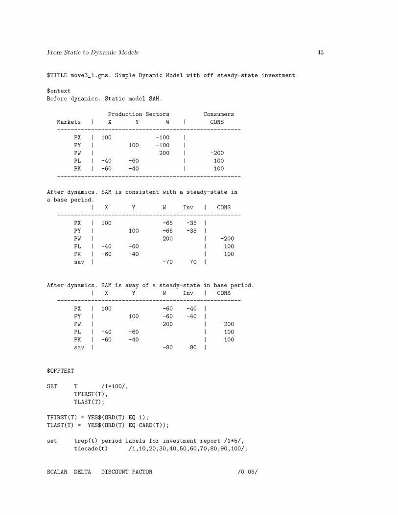
$TITLE move3_1.gms. Simple Dynamic Model with off steady-state investment
$ontextBefore dynamics. Static model SAM.
Production Sectors ConsumersMarkets | X Y W | CONS------------------------------------------------------
PX | 100 -100 |PY | 100 -100 |PW | 200 | -200PL | -40 -60 | 100PK | -60 -40 | 100
------------------------------------------------------
After dynamics. SAM is consistent with a steady-state ina base period.
| X Y W Inv | CONS------------------------------------------------------
PX | 100 -65 -35 |PY | 100 -65 -35 |PW | 200 | -200PL | -40 -60 | 100PK | -60 -40 | 100sav | -70 70 |
After dynamics. SAM is away of a steady-state in base period.| X Y W Inv | CONS
------------------------------------------------------PX | 100 -60 -40 |PY | 100 -60 -40 |PW | 200 | -200PL | -40 -60 | 100PK | -60 -40 | 100sav | -80 80 |
$OFFTEXT
SET T /1*100/,TFIRST(T),TLAST(T);
TFIRST(T) = YES$(ORD(T) EQ 1);TLAST(T) = YES$(ORD(T) EQ CARD(T));
set trep(t) period labels for investment report /1*5/,tdecade(t) /1,10,20,30,40,50,60,70,80,90,100/;
SCALAR DELTA DISCOUNT FACTOR /0.05/
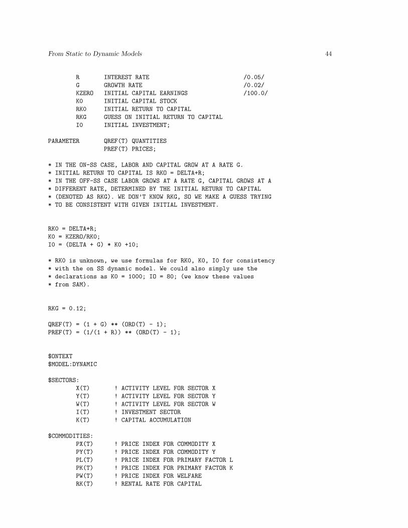
From Static to Dynamic Models 44
R INTEREST RATE /0.05/G GROWTH RATE /0.02/KZERO INITIAL CAPITAL EARNINGS /100.0/K0 INITIAL CAPITAL STOCKRK0 INITIAL RETURN TO CAPITALRKG GUESS ON INITIAL RETURN TO CAPITALI0 INITIAL INVESTMENT;
PARAMETER QREF(T) QUANTITIESPREF(T) PRICES;
* IN THE ON-SS CASE, LABOR AND CAPITAL GROW AT A RATE G.* INITIAL RETURN TO CAPITAL IS RKO = DELTA+R;* IN THE OFF-SS CASE LABOR GROWS AT A RATE G, CAPITAL GROWS AT A* DIFFERENT RATE, DETERMINED BY THE INITIAL RETURN TO CAPITAL* (DENOTED AS RKG). WE DON’T KNOW RKG, SO WE MAKE A GUESS TRYING* TO BE CONSISTENT WITH GIVEN INITIAL INVESTMENT.
RK0 = DELTA+R;K0 = KZERO/RK0;I0 = (DELTA + G) * K0 +10;
* RK0 is unknown, we use formulas for RK0, K0, I0 for consistency* with the on SS dynamic model. We could also simply use the* declarations as K0 = 1000; IO = 80; (we know these values* from SAM).
RKG = 0.12;
QREF(T) = (1 + G) ** (ORD(T) - 1);PREF(T) = (1/(1 + R)) ** (ORD(T) - 1);
$ONTEXT$MODEL:DYNAMIC
$SECTORS:X(T) ! ACTIVITY LEVEL FOR SECTOR XY(T) ! ACTIVITY LEVEL FOR SECTOR YW(T) ! ACTIVITY LEVEL FOR SECTOR WI(T) ! INVESTMENT SECTORK(T) ! CAPITAL ACCUMULATION
$COMMODITIES:PX(T) ! PRICE INDEX FOR COMMODITY XPY(T) ! PRICE INDEX FOR COMMODITY YPL(T) ! PRICE INDEX FOR PRIMARY FACTOR LPK(T) ! PRICE INDEX FOR PRIMARY FACTOR KPW(T) ! PRICE INDEX FOR WELFARERK(T) ! RENTAL RATE FOR CAPITAL
From Static to Dynamic Models 45
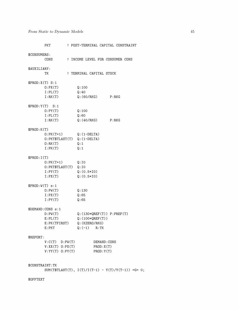
PKT ! POST-TERMINAL CAPITAL CONSTRAINT
$CONSUMERS:CONS ! INCOME LEVEL FOR CONSUMER CONS
$AUXILIARY:TK ! TERMINAL CAPITAL STOCK
$PROD:X(T) S:1O:PX(T) Q:100I:PL(T) Q:40I:RK(T) Q:(60/RKG) P:RKG
$PROD:Y(T) S:1O:PY(T) Q:100I:PL(T) Q:60I:RK(T) Q:(40/RKG) P:RKG
$PROD:K(T)O:PK(T+1) Q:(1-DELTA)O:PKT$TLAST(T) Q:(1-DELTA)O:RK(T) Q:1I:PK(T) Q:1
$PROD:I(T)O:PK(T+1) Q:I0O:PKT$TLAST(T) Q:I0I:PY(T) Q:(0.5*I0)I:PX(T) Q:(0.5*I0)
$PROD:W(T) s:1O:PW(T) Q:130I:PX(T) Q:65I:PY(T) Q:65
$DEMAND:CONS s:1D:PW(T) Q:(130*QREF(T)) P:PREF(T)E:PL(T) Q:(100*QREF(T))E:PK(TFIRST) Q:(KZERO/RKG)E:PKT Q:(-1) R:TK
$REPORT:V:C(T) D:PW(T) DEMAND:CONSV:XX(T) O:PX(T) PROD:X(T)V:YY(T) O:PY(T) PROD:Y(T)
$CONSTRAINT:TKSUM(T$TLAST(T), I(T)/I(T-1) - Y(T)/Y(T-1)) =G= 0;
$OFFTEXT

From Static to Dynamic Models 46
$SYSINCLUDE MPSGESET DYNAMIC
X.L(T) = QREF(T);Y.L(T) = QREF(T);W.L(T) = QREF(T);I.L(T) = QREF(T);K.L(T) = K0*QREF(T);TK.L = K0 * (1 + G) ** CARD(T);
PX.L(T) = PREF(T);PY.L(T) = PREF(T);PL.L(T) = PREF(T);PK.L(T) = (1+R)*PREF(T);PW.L(T) = PREF(T);RK.L(T) = RKG*PREF(T);PKT.L = SUM(TLAST, PK.L(TLAST)/(1+R));
SET ITER JACOBI-SECANT ITERATIONS / ITER1*ITER6/;
PARAMETERINVEST INVESTMENT PATHINTRATE INTEREST RATECONSUM CONSUMPTION LEVELGROWTH CONSUMPTION GROWTH RATEERROR ERROR ESTIMATE BY ITERATIONRK0VAL VALUE OF RK0;
LOOP(ITER,
$INCLUDE DYNAMIC.GENSOLVE DYNAMIC USING MCP;
INVEST(TREP,ITER) = I.L(TREP) * I0;INTRATE(TFIRST,ITER) = RKG-DELTA;INTRATE(T+1,ITER)$PX.L(T+1) = PX.L(T)/PX.L(T+1) - 1;CONSUM(T,ITER) = C.L(T);
* ERROR(ITER) = C.L("1") - (200-I0);* ERROR(ITER) = I.L("1")*I0 - I0;
ERROR(ITER) = C.L("1") - (XX.L("1")+YY.L("1")-I0);RK0VAL(ITER) = RKG;
IF (ORD(ITER)-1,RKG = RKG + ERROR(ITER)/(ERROR(ITER-1)-ERROR(ITER))
* (RK0VAL(ITER)-RK0VAL(ITER-1));ELSE
RKG = RKG + 0.01;);
);INVEST(TREP,"I0") = I0;DISPLAY INVEST, INTRATE, CONSUM;
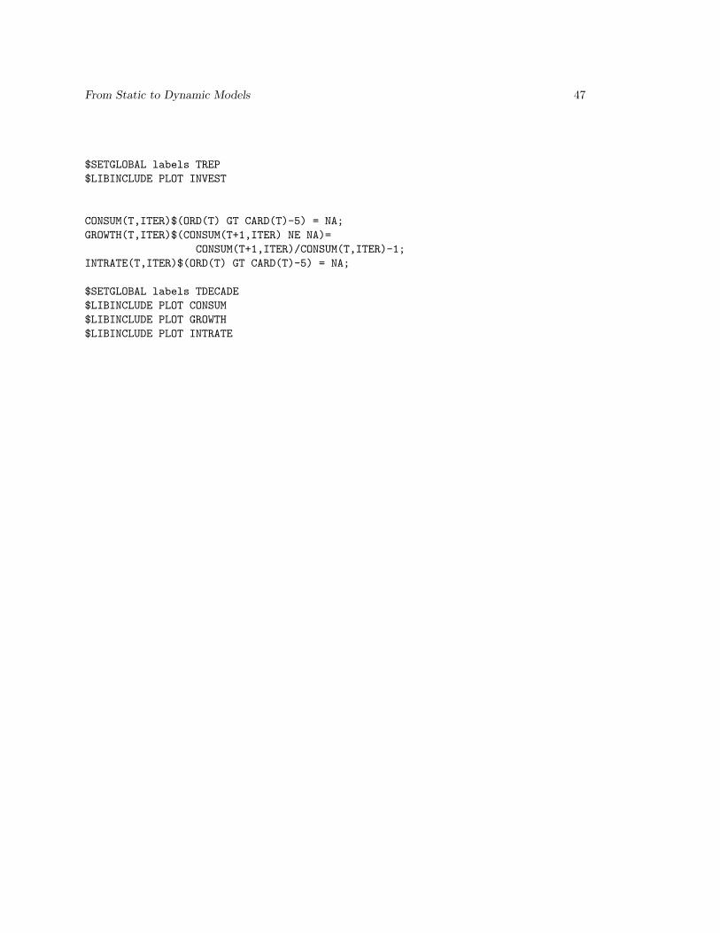
From Static to Dynamic Models 47
$SETGLOBAL labels TREP$LIBINCLUDE PLOT INVEST
CONSUM(T,ITER)$(ORD(T) GT CARD(T)-5) = NA;GROWTH(T,ITER)$(CONSUM(T+1,ITER) NE NA)=
CONSUM(T+1,ITER)/CONSUM(T,ITER)-1;INTRATE(T,ITER)$(ORD(T) GT CARD(T)-5) = NA;
$SETGLOBAL labels TDECADE$LIBINCLUDE PLOT CONSUM$LIBINCLUDE PLOT GROWTH$LIBINCLUDE PLOT INTRATE

From Static to Dynamic Models 48
Appendix 4. Dynamic GTAP
Appendix 4 contains Rutherford’s version of dynamic GTAP.
$title A Forward-Looking GTAP Model
scalar debug Switch for debugging with steady-state calibration /0/;
set t Time periods (annual steps) /1995*2080/t0(t) First period of the model /1995/,tl(t) Final period of the model /2080/,decade(t) Decade identifiers /2000, 2010, 2020, 2030, 2040, 2050,
2060, 2070, 2080 /;
parameter year(t); year(t) = 1995 + (ord(t)-1);
scalaresubt Intertemporal elasticity of substitution /0.5/depr Annual depreciation rate /0.07/gterm Baseline (long-run) growth rate /0.02/r0 Benchmark interest rate /0.05/,pk0 Benchmark capital pricesrvshr Single period survival sharetermcap Terminal period capital;
* ======================================================================* Calibration of savings and investment to a uniform steady-state* equilibrium across all regions:
pk0 = 1 + r0;
* ======================================================================* Read the dataset and define regional affiliations and baseline* growth rates:
$libinclude mrtdata shock
SCALAResubdm Elasticity of substitution - domestic vs. imports / 4 /,esubmm Elasticity of substitution - imports / 8 /;
parameter gr0(r) Base year growth rate /
DNK 0.02, USA 0.02, OOE 0.01, ASI 0.08, JPN 0.04, CHN 0.05, FSU 0.05, ROW 0.04/,
gr(t,r) Growth rates through the model horizon;
* First pass: check steady-state consistency:
if (debug, gr0(r) = gterm;);
parameterqref(t,r) Reference quantity path
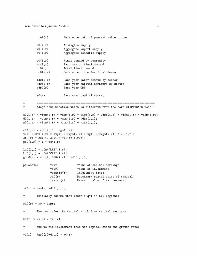
From Static to Dynamic Models 49
pref(t) Reference path of present value prices
a0(i,r) Armington supplym0(i,r) Aggregate import supplyd0(i,r) Aggregate domestic supply
c0(i,r) Final demand by commoditytc(i,r) Tax rate on final demandct0(r) Total final demandpc0(i,r) Reference price for final demand
ld0(i,r) Base year labor demand by sectorkd0(i,r) Base year capital earnings by sectorgdp0(r) Base year GDP
k0(r) Base year capital stock;
* ======================================================================* Adopt some notation which is different from the core GTAPinGAMS model:
a0(i,r) = vipm(i,r) + vdpm(i,r) + vigm(i,r) + vdgm(i,r) + vifm(i,r) + vdfm(i,r);d0(i,r) = vdpm(i,r) + vdgm(i,r) + vdfm(i,r);m0(i,r) = vipm(i,r) + vigm(i,r) + vifm(i,r);
c0(i,r) = vpm(i,r) + vgm(i,r);tc(i,r)$c0(i,r) = (tp(i,r)*vpm(i,r) + tg(i,r)*vgm(i,r)) / c0(i,r);ct0(r) = sum(i, c0(i,r)*(1+tc(i,r)));pc0(i,r) = 1 + tc(i,r);
ld0(i,r) = vfm("LAB",i,r);kd0(i,r) = vfm("CAP",i,r);gdp0(r) = sum(i, ld0(i,r) + kd0(i,r));
parameter vk(r) Value of capital earningsvi(r) Value of investmentviratio(r) Investment ratiork0(r) Benchmark rental price of capitaltaxrev(r) Present value of tax revenue;
vk(r) = sum(i, kd0(i,r));
* Initially assume that Tobin’s q=1 in all regions:
rk0(r) = r0 + depr;
* Then we infer the capital stock from capital earnings:
k0(r) = vk(r) / rk0(r);
* and we fix investment from the capital stock and growth rate:
vi(r) = (gr0(r)+depr) * k0(r);

From Static to Dynamic Models 50
parameter profit;profit(r,i) = vom(i,r) * (1-ty(i,r)) - sum(j, vafm(j,i,r)*(1+ti(j,i,r)))
- ld0(i,r) - kd0(i,r);display profit;
parameter c0adj Increment in consumption for investment,i0adj Increment in investment to match benchmarklamda Adjustment scaling factor;
c0adj(r) = max(0, vom("cgd",r)-vi(r));i0adj(r) = max(0, vi(r)-vom("cgd",r));
lamda(r) = (1-ty("cgd",r))*i0adj(r)/sum(i, c0(i,r)*pai0(i,"cgd",r));vafm(i,"cgd",r) = vafm(i,"cgd",r) + lamda(r) * c0(i,r);c0(i,r) = c0(i,r) * (1 - lamda(r));
* Investment exceeds the target -- move some of the investment* demand into final demand:
lamda(r) = (1-ty("cgd",r)) * c0adj(r) / sum(i, vafm(i,"cgd",r)*pai0(i,"cgd",r));c0(i,r) = c0(i,r) + lamda(r) * vafm(i,"cgd",r);vafm(i,"cgd",r) = vafm(i,"cgd",r) * (1 - lamda(r));
ct0(r) = sum(i, c0(i,r) * pc0(i,r));vom(cgd,r) = vi(r);
profit(r,i) = vom(i,r) * (1-ty(i,r)) - sum(j, vafm(j,i,r)*(1+ti(j,i,r)))- ld0(i,r) - kd0(i,r);
display c0adj, i0adj;display profit;
parameter gdp(t,r) Relative GDP indexeff(t,i,r) Efficiency index (adjustment factor)ieff(t,r) Investment efficiency index (shock parameter)keff(t,r) Capital efficiency index (shock parameter);
ieff(t,r) = 1;keff(t,r) = 1;
$ontext$model:gtap
$sectors:c(t,r) ! Private consumptiony(i,t,r)$vom(i,r) ! Outputa(i,t,r)$a0(i,r) ! Armington aggregation of domestic and importsk(t,r) ! Capital stockinv(t,r) ! Investmentyt(t) ! Transport
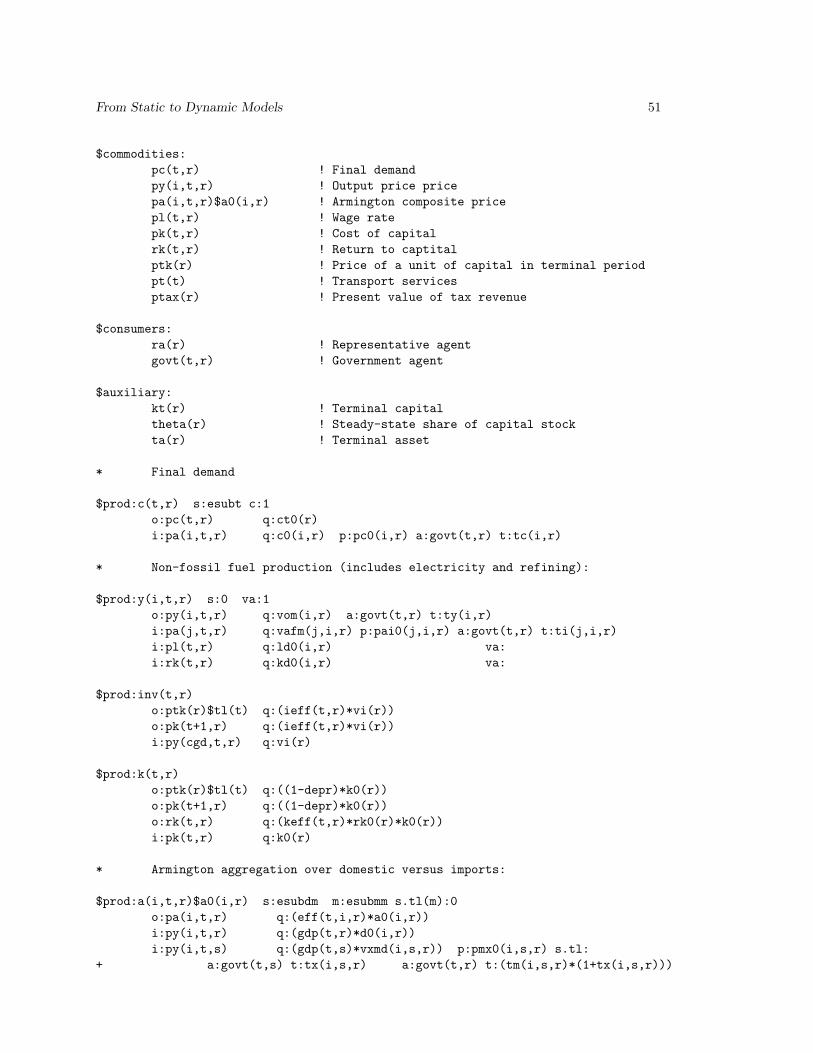
From Static to Dynamic Models 51
$commodities:pc(t,r) ! Final demandpy(i,t,r) ! Output price pricepa(i,t,r)$a0(i,r) ! Armington composite pricepl(t,r) ! Wage ratepk(t,r) ! Cost of capitalrk(t,r) ! Return to captitalptk(r) ! Price of a unit of capital in terminal periodpt(t) ! Transport servicesptax(r) ! Present value of tax revenue
$consumers:ra(r) ! Representative agentgovt(t,r) ! Government agent
$auxiliary:kt(r) ! Terminal capitaltheta(r) ! Steady-state share of capital stockta(r) ! Terminal asset
* Final demand
$prod:c(t,r) s:esubt c:1o:pc(t,r) q:ct0(r)i:pa(i,t,r) q:c0(i,r) p:pc0(i,r) a:govt(t,r) t:tc(i,r)
* Non-fossil fuel production (includes electricity and refining):
$prod:y(i,t,r) s:0 va:1o:py(i,t,r) q:vom(i,r) a:govt(t,r) t:ty(i,r)i:pa(j,t,r) q:vafm(j,i,r) p:pai0(j,i,r) a:govt(t,r) t:ti(j,i,r)i:pl(t,r) q:ld0(i,r) va:i:rk(t,r) q:kd0(i,r) va:
$prod:inv(t,r)o:ptk(r)$tl(t) q:(ieff(t,r)*vi(r))o:pk(t+1,r) q:(ieff(t,r)*vi(r))i:py(cgd,t,r) q:vi(r)
$prod:k(t,r)o:ptk(r)$tl(t) q:((1-depr)*k0(r))o:pk(t+1,r) q:((1-depr)*k0(r))o:rk(t,r) q:(keff(t,r)*rk0(r)*k0(r))i:pk(t,r) q:k0(r)
* Armington aggregation over domestic versus imports:
$prod:a(i,t,r)$a0(i,r) s:esubdm m:esubmm s.tl(m):0o:pa(i,t,r) q:(eff(t,i,r)*a0(i,r))i:py(i,t,r) q:(gdp(t,r)*d0(i,r))i:py(i,t,s) q:(gdp(t,s)*vxmd(i,s,r)) p:pmx0(i,s,r) s.tl:
+ a:govt(t,s) t:tx(i,s,r) a:govt(t,r) t:(tm(i,s,r)*(1+tx(i,s,r)))

From Static to Dynamic Models 52
i:pt(t)#(s) q:(gdp(t,s)*vtwr(i,s,r)) p:pmt0(i,s,r) s.tl:+ a:govt(t,r) t:tm(i,s,r)
* International transport services (Cobb-Douglas):
$prod:yt(t) s:1o:pt(t) q:(sum((i,r), vst(i,r)))i:py(i,t,r) q:vst(i,r)
* Final demand:
$demand:ra(r) s:esubtd:pc(t,r) q:(ct0(r)*qref(t,r)) p:pref(t)e:ptk(r) q:(-k0(r)) r:kt(r)
* value of base year trade balance:
e:pc(t,"usa") q:(vb(r)*qref(t,r))e:pl(t,r) q:(evoa("lab",r)*qref(t,r))
e:pl(t0,"usa") q:(-1) r:ta(r)e:pk(t0,r) q:k0(r)
e:ptax(r) q:taxrev(r)
$demand:govt(t,r)d:ptax(r)
$constraint:kt(r)sum(t$tl(t+1), c(t,r)*inv(t+1,r) - c(t+1,r)*inv(t,r)) =e= 0;
* Region r share of aggregate assets:
$constraint:theta(r)theta(r) * sum((tl,rr), c(tl,rr)*pc(tl,rr)*ct0(rr)
- evoa("lab",rr)*qref(tl,rr)*pl(tl,rr)- vb(rr)*qref(tl,rr)*pc(tl,"usa"))=e= sum(tl, c(tl,r)*pc(tl,r)*ct0(r)
- evoa("lab",r)*qref(tl,r)*pl(tl,r)- vb(r)*qref(tl,r)*pc(tl,"usa"));
* Terminal asset adjustment:
$constraint:ta(r)sum(t0, pl(t0,"usa")) * ta(r) =e=theta(r) * sum(rr,ptk(rr)*kt(rr)*k0(rr)) - ptk(r)*kt(r)*k0(r);
$offtext$sysinclude mpsgeset gtap
* Growth rates through the horizon:

From Static to Dynamic Models 53
scalar ssyear /2060/;
set tss(t); tss(t) = yes$(year(t) ge ssyear);gr(t,r)$(not tss(t)) = gterm * (year(t)-1995)/(ssyear-1995) +
gr0(r) * (ssyear-year(t))/(ssyear-1995);gr(tss,r) = gterm;
*$setglobal gp_xl decade*$libinclude gnuplot gr
qref(t,r) = 1;loop(t, qref(t+1,r) = qref(t,r) * (1 + gr(t,r)););
* Generate an index to control Armington demand structure:
gdp(t,r) = ( qref(t,r) * gdp0(r) / sum(rr, qref(t,rr)*gdp0(rr)) ) /( gdp0(r) / sum(rr, gdp0(rr)) );
eff(t,i,r)$a0(i,r) = ( gdp(t,r)*d0(i,r) +sum(s, gdp(t,s) *
(vxmd(i,s,r)*pmx0(i,s,r)+ vtwr(i,s,r)*pmt0(i,s,r))) ) / a0(i,r);display gdp, eff;
pref(t) = (1/(1+r0))**(ord(t)-1);pref(t) = pref(t) / sum(t0, pref(t0));
pc.l(t,r) = pref(t);py.l(i,t,r) = pref(t);pa.l(i,t,r) = pref(t);pl.l(t,r) = pref(t);pk.l(t,r) = pk0 * pref(t);rk.l(t,r) = pref(t);ptk.l(r) = sum(t$tl(t),pk.l(t,r))/(1+r0);pt.l(t) = pref(t);
c.l(t,r) = qref(t,r);y.l(i,t,r) = qref(t,r);a.l(i,t,r) = qref(t,r);
k.l(t,r) = qref(t,r);inv.l(t,r) = qref(t,r);yt.l(t) = qref(t,"usa");
kt.l(r) = sum(tl, qref(tl,r))*(1 + gterm);
* Replicate the 1995 calibrated benchmark -- the deviation should be* on the order of 1e-5:
if (debug,gtap.iterlim = 0;
elsevb(r) = 0;

From Static to Dynamic Models 54
);
ta.lo(r) = -inf;theta.lo(r) = -inf;
theta.l(r) = sum(tl, c.l(tl,r)*pc.l(tl,r)*ct0(r)- evoa("lab",r)*qref(tl,r)*pl.l(tl,r)- vb(r)*qref(tl,r)*pc.l(tl,"usa")) /
sum((tl,rr), c.l(tl,rr)*pc.l(tl,rr)*ct0(rr)- evoa("lab",rr)*qref(tl,rr)*pl.l(tl,rr)- vb(rr)*qref(tl,rr)*pc.l(tl,"usa"));
taxrev(r) = sum(t, qref(t,r) * pref(t) *(sum((i,s), gdp(t,s) * tm(i,s,r)*( vtwr(i,s,r) +vxmd(i,s,r)*(1+tx(i,s,r)) )+ gdp(t,r) * tx(i,r,s) * vxmd(i,r,s) ) +sum((i,j), ti(j,i,r)*vafm(j,i,r)) +sum(i, ty(i,r) * vom(i,r)) +sum(i, tc(i,r) * c0(i,r)) ));
$include gtap.gensolve gtap using mcp;
abort$debug "Benchmark precision:", gtap.objval;
parameter capital(t,r) Capital growth rateconsum(t,r) Consumption levelinterest(t,r) Interate rate (%);
capital(t,r) = 100 * (k.l(t+1,r)/k.l(t,r) - 1);consum(t,r) = 100 * (c.l(t+1,r)/c.l(t,r) - 1);interest(t,r)$(not tl(t)) = 100 * (pc.l(t,r)/pc.l(t+1,r)-1);
capital(tl,r) = na;consum(tl,r) = na;interest(tl,r) = na;
parameter tasum Check sum for terminal assets;tasum = sum(r,ta.l(r)); display tasum;
display capital, consum, interest;
*.$setglobal gp_xl decade*.$libinclude gnuplot capital*.$libinclude gnuplot consum*.$libinclude gnuplot interest
parameterassets(t,*) Beginning of period assetsborrow(*,*) Net borrowing by periodpvdebt(*,*) Present value of debtfvdebt(*,*) Future value of debt;

From Static to Dynamic Models 55
* Net borrowing from abroad equals
pvdebt(t,r) = 0;assets(t0,r) = pk.l(t0,r)*k.l(t0,r)*k0(r);borrow(t,r) = pc.l(t,r)*c.l(t,r)*ct0(r) + py.l("cgd",t,r)*inv.l(t,r)*vi(r)
- pl.l(t,r)*evoa("lab",r)*qref(t,r)- rk.l(t,r)*rk0(r)*k0(r)*k.l(t,r)- govt.l(t,r);
loop(t,pvdebt(t+1,r) = pvdebt(t,r) + borrow(t,r);assets(t+1,r) = pk.l(t+1,r)*k.l(t+1,r)*k0(r) - pvdebt(t,r);
);
fvdebt(t,r) = pvdebt(t,r)/pc.l(t,"usa");
loop(t0,assets(t,r) = assets(t,r)/pc.l(t0,"usa");borrow(t,r) = borrow(t,r)/pc.l(t0,"usa");pvdebt(t,r) = pvdebt(t,r)/pc.l(t0,"usa"););
*.$libinclude gnuplot assets*.$libinclude gnuplot borrow*.$libinclude gnuplot pvdebt*.$libinclude gnuplot fvdebt
borrow(t,"chk") = sum(r, borrow(t,r));pvdebt(t,"chk") = sum(r, pvdebt(t,r));display assets, borrow, pvdebt, fvdebt;
borrow(t,"chk") = 0;pvdebt(t,"chk") = 0;