motivation when we do word processing, graphics, spreadsheets, games etc, we let the operating...

MotivationMotivation

When we do word processing, graphics, spreadsheets, games etc, we let the operating system take charge of saving and retrieving files. However, for databases, we will bypass the operating system and take care of file input/output (I/O) ourselves. Why?

• Speed

• Reliability

• Scalability (addressability, files can’t span disks)

• Portability

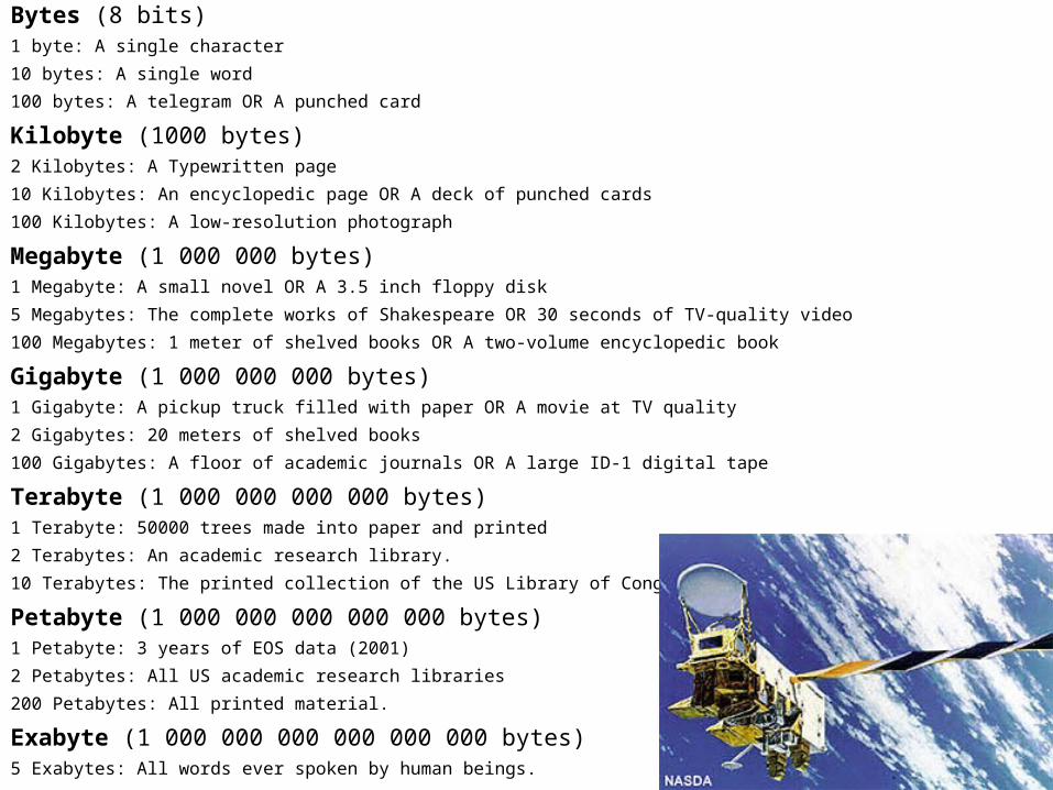
Bytes (8 bits)1 byte: A single character

10 bytes: A single word

100 bytes: A telegram OR A punched card

Kilobyte (1000 bytes)2 Kilobytes: A Typewritten page

10 Kilobytes: An encyclopedic page OR A deck of punched cards

100 Kilobytes: A low-resolution photograph

Megabyte (1 000 000 bytes)1 Megabyte: A small novel OR A 3.5 inch floppy disk

5 Megabytes: The complete works of Shakespeare OR 30 seconds of TV-quality video

100 Megabytes: 1 meter of shelved books OR A two-volume encyclopedic book

Gigabyte (1 000 000 000 bytes)1 Gigabyte: A pickup truck filled with paper OR A movie at TV quality

2 Gigabytes: 20 meters of shelved books

100 Gigabytes: A floor of academic journals OR A large ID-1 digital tape

Terabyte (1 000 000 000 000 bytes)1 Terabyte: 50000 trees made into paper and printed

2 Terabytes: An academic research library.

10 Terabytes: The printed collection of the US Library of Congress

Petabyte (1 000 000 000 000 000 bytes)1 Petabyte: 3 years of EOS data (2001)

2 Petabytes: All US academic research libraries

200 Petabytes: All printed material.

Exabyte (1 000 000 000 000 000 000 bytes)5 Exabytes: All words ever spoken by human beings.

Classification of Physical Storage MediaClassification of Physical Storage Media

• Speed with which data can be accessed• Cost per unit of data• Reliability

– data loss on power failure or system crash

– physical failure of the storage device

• Can differentiate storage into:– volatile storage: loses contents when power is switched off

– non-volatile storage: • Contents persist even when power is switched off.

• Includes secondary and tertiary storage, as well as batter-backed up main-memory.

1 1 0 1 1 0 0 0

Physical Storage MediaPhysical Storage Media

• Cache – fastest and most costly form of storage; volatile; managed by the computer system hardware.

• Main memory:– fast access (10s to 100s of nanoseconds; 1 nanosecond = 10–9

seconds)

– generally too small (or too expensive) to store the entire database

• capacities of up to a few Gigabytes widely used currently

• Capacities have gone up and per-byte costs have decreased steadily and rapidly (roughly factor of 2 every 2 to 3 years)

– Volatile — contents of main memory are usually lost if a power failure or system crash occurs.

Physical Storage Media (Cont.)Physical Storage Media (Cont.)• Flash memory

– Data survives power failure

– Data can be written at a location only once, but location can be erased and written to again

• Can support only a limited number of write/erase cycles.

• Erasing of memory has to be done to an entire bank of memory

– Reads are roughly as fast as main memory

– But writes are slow (few microseconds), erase is slower

– Cost per unit of storage roughly similar to main memory

– Widely used in embedded devices such as digital cameras

– also known as EEPROM (Electrically Erasable Programmable Read-Only Memory)We will i

gnore this type of m

emory for this c

lass

Physical Storage Media (Cont.)Physical Storage Media (Cont.)• Magnetic-disk

– Data is stored on spinning disk, and read/written magnetically

– Primary medium for the long-term storage of data; typically stores entire database.

– Data must be moved from disk to main memory for access, and written back for storage• Much slower access than main memory (more on this later)

– direct-access – possible to read data on disk in any order, unlike magnetic tape

– Capacities range up to roughly 200 GB currently• Much larger capacity and cost/byte than main memory/flash memory

• Growing constantly and rapidly with technology improvements (factor of 2 to 3 every 2 years)

– Survives power failures and system crashes• disk failure can destroy data, but is very rare

Physical Storage Media (Cont.)Physical Storage Media (Cont.)

• Optical storage – non-volatile, data is read optically from a spinning disk

using a laser – CD-ROM (640 - 800 MB) and DVD (4.7 to 17 GB) most

popular forms– Write-one, read-many (WORM) optical disks used for

archival storage (CD-R and DVD-R)– Multiple write versions also available (CD-RW, DVD-

RW, and DVD-RAM)– Reads and writes are slower than with magnetic disk – Juke-box systems, with large numbers of removable

disks, a few drives, and a mechanism for automatic loading/unloading of disks available for storing large volumes of data

Physical Storage Media (Cont.)Physical Storage Media (Cont.)

• Tape storage – non-volatile, used primarily for backup (to

recover from disk failure), and for archival data– sequential-access – much slower than disk – very high capacity (40 to 300 GB tapes available)– tape can be removed from drive storage costs

much cheaper than disk, but drives are expensive– Tape jukeboxes available for storing massive

amounts of data • hundreds of terabytes (1 terabyte = 109 bytes) to even

a petabyte (1 petabyte = 1012 bytes)

Storage HierarchyStorage HierarchyPrimary storage:

Fastest media but volatile

(cache, main memory)

Primary storage:

Fastest media but volatile

(cache, main memory)

Secondary storage: next

level in hierarchy, non-volatile,

moderately fast access time(also called on-line storage)

Secondary storage: next

level in hierarchy, non-volatile,

moderately fast access time(also called on-line storage)

Tertiary storage: lowest

level in hierarchy, non-volatile, slow

access time (also called off-line storage)

Tertiary storage: lowest

level in hierarchy, non-volatile, slow

access time (also called off-line storage)

CPU

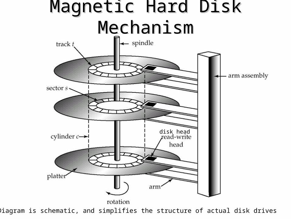
Magnetic Hard Disk MechanismMagnetic Hard Disk Mechanism

NOTE: Diagram is schematic, and simplifies the structure of actual disk drives

disk head

Track: The green ring

Cylinder: The yellow “tube”

Sector: The “pizza slice”

Block: The blue intersection of a track and sector

Block size is a multiple of sector size, (which is fixed) in this example the multiple is one

Notion of Notion of “closeness” “closeness” for a hard for a hard

drivedrive

1 2

3

456

7

8

9 10

11

12

16

15

17 18

19

20

24

23Note direction of rotation

Where should 25 go?

This notion of closeness is very important, and we should try to exploit it where possible I.

Suppose we fill a hard drive with a million records. We could organize them such that the ith record is close to the ith + 1 record.

If we retrieve them in order from 1 to one million, we can do this is X time.(this is called a sequential scan, or a linear scan)

If instead we retrieve them in random order it will take in class times longer.

•`Next’ block concept: blocks on same track, followed by

blocks on same cylinder, followed by

blocks on adjacent cylinder




This notion of closeness is very important, and we should try to exploit it where possible II.

If we know we are going to do a sequential scan, we may even be able to do prefetching. This can make a huge difference.







Magnetic DisksMagnetic Disks• Read-write head

– Positioned very close to the platter surface (almost touching it)– Reads or writes magnetically encoded information.

• Surface of platter divided into circular tracks– Over 16,000 tracks per platter on typical hard disks

• Each track is divided into sectors. – A sector is the smallest unit of data that can be read or written.– Sector size typically 512 bytes– Typical sectors per track: 200 (on inner tracks) to 400 (on outer tracks)

• To read/write a sector– disk arm swings to position head on right track– platter spins continually; data is read/written as sector passes under head

• Head-disk assemblies – multiple disk platters on a single spindle (typically 2 to 4)– one head per platter, mounted on a common arm.

• Cylinder i consists of ith track of all the platters

Magnetic Disks (Cont.)Magnetic Disks (Cont.)• Earlier generation disks were susceptible to head-crashes

– Surface of earlier generation disks had metal-oxide coatings which would disintegrate on head crash and damage all data on disk

– Current generation disks are less susceptible to such disastrous failures, although individual sectors may get corrupted

• Disk controller – interfaces between the computer system and the disk drive hardware.– accepts high-level commands to read or write a sector – initiates actions such as moving the disk arm to the right track and

actually reading or writing the data– Computes and attaches checksums to each sector to verify that data

is read back correctly• If data is corrupted, with very high probability stored checksum won’t

match recomputed checksum

– Ensures successful writing by reading back sector after writing it– Performs remapping of bad sectors

0 1 0 1 1 1 1 0 1

A very simple checksum:Single parity check code. This code appends to each K data bits an additional bit whose value is taken to make number of bits even

0 1 0 1 1 1 1 0 ?We want to record the message “01011110” to the disk.

We set the ninth bit (the checksum bit) to whatever value makes the number of bits (all nine of them) to be even.

Suppose that the first bit gets flipped by mistake…

We can tell that one bit was flipped (one or three or five…)

1 1 0 1 1 1 1 0 1

Although we can not tell which one...

Suppose we have no parity bit, and we want to store 8 bitsP{single bit error} = pP{no error in single bit} = (1 – p)P{no error in 8 bits} = (1 – p)8

P{unseen error in 8 bits} = 1 - (1 – p)8

= 7.9 10-4

Suppose instead we have 1 parity bit per 8 bitsP{no error in single bit} = (1 – p)P{no error in 9 bits} = (1 – p)9

P{single error in 9 bits} = 9(P{single bit error} P{no error in 8 other bits} ) = 9p(1 – p)8

P{unseen error in 9 bits} = 1 - P{no error in 9 bits} - P{single error in 9 bits} = 1 – (1 – p)9 – 9p(1 – p)8

= 3.6 10-7

Suppose that the probability of a bit being in error is p = 10-4

Suppose that the probability of a bit being in error is p = 10-4

We are about 2194 times less likely to have an error go unnoticed.

Disk Subsystem

• Multiple disks connected to a computer system through a controller– Controllers functionality (checksum, bad sector remapping) often

carried out by individual disks; reduces load on controller

• Disk interface standards families– ATA (AT adaptor) range of standards – SCSI (Small Computer System Interconnect) range of standards– Several variants of each standard (different speeds and capabilities)

Performance Measures of DisksPerformance Measures of Disks• Access time – the time it takes from when a read or write request is

issued to when data transfer begins. Consists of: – Seek time – time it takes to reposition the arm over the correct track.

• Average seek time is 1/2 the worst case seek time.

• 4 to 10 milliseconds on typical disks

– Rotational delay (Rotational latency) – time it takes for the sector to be accessed to appear under the head. • Average latency is 1/2 of the worst case latency.

• 4 to 11 milliseconds on typical disks (5400 to 15000 r.p.m.)

– Transfer time – the rate at which data can be retrieved from or stored to the disk.• 4 to 8 MB per second is typical

Seek time and rotational delay dominate, and we can do some things to help (in the context of databases). Transfer time is less important, and in any case, there is nothing we can really do about it.

Performance Measures (Cont.)Performance Measures (Cont.)

• Mean time to failure (MTTF) – the average time the disk is expected to run continuously without any failure.– Typically 3 to 5 years– Probability of failure of new disks is quite low,

corresponding to a“theoretical MTTF” of 30,000 to 1,200,000 hours for a new disk

• E.g., an MTTF of 1,200,000 hours for a new disk means that given 1000 relatively new disks, on an average one will fail every 1200 hours

– MTTF decreases as disk ages!!

Optimization of Disk-Block AccessOptimization of Disk-Block Access• Block – a contiguous sequence of sectors from a

single track – data is transferred between disk and main memory in

blocks (i.e, you can’t ask for a single bit)• Smaller blocks: more transfers from disk

• Larger blocks: more space wasted due to partially filled blocks

• Typical block sizes today range from 4 to 16 kilobytes

• Disk-arm-scheduling algorithms order pending accesses to tracks so that disk arm movement is minimized – elevator algorithm : move disk arm in one direction (from

outer to inner tracks or vice versa), processing next request in that direction, till no more requests in that direction, then reverse direction and repeat

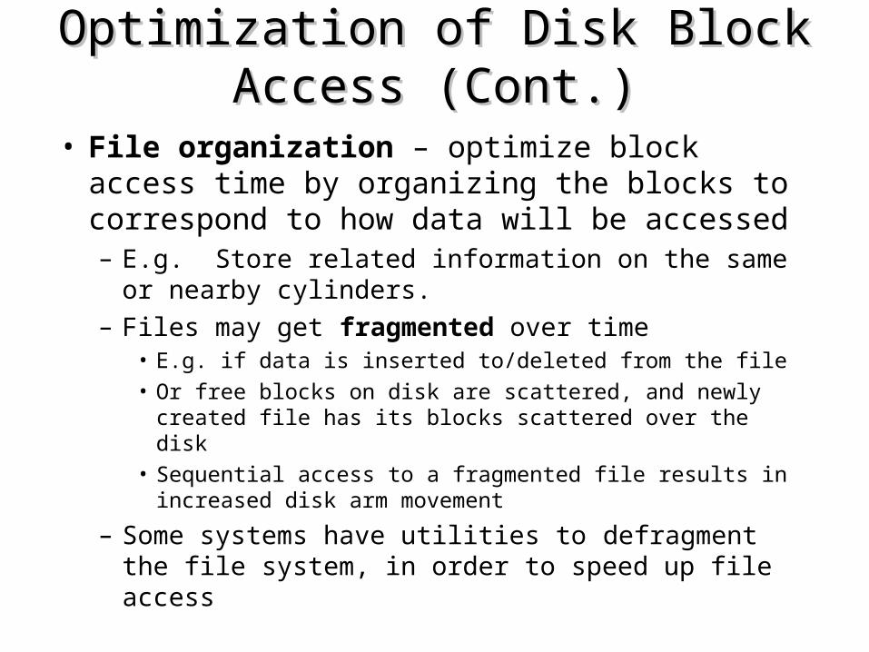
Optimization of Disk Block Access (Cont.)Optimization of Disk Block Access (Cont.)

• File organization – optimize block access time by organizing the blocks to correspond to how data will be accessed– E.g. Store related information on the same or nearby

cylinders.

– Files may get fragmented over time• E.g. if data is inserted to/deleted from the file

• Or free blocks on disk are scattered, and newly created file has its blocks scattered over the disk

• Sequential access to a fragmented file results in increased disk arm movement

– Some systems have utilities to defragment the file system, in order to speed up file access

Backup DisksBackup Disks

0 1 0 1 1 1 1 0

Suppose we have critical data in our database, and we want to back it up…

We can use another hard drive of the same size to back up the data. This is typically called mirroring or shadowing.

Suppose we want to back up two disks, or sixteen disks. How many backup disks do we need?

Hard drive

0 1 0 1 1 1 1 0

Mirror drive

Backup Disks: Parity Scheme IBackup Disks: Parity Scheme I

0 1 0 1 1 1 1 0

Suppose we want to backup 4 hard drives, we can do this with just one hard drive of equal size!!!

Consider just the first bit for a moment….

We count all the bits in the first position that are 1’s. If this number is odd, then the first bit of the check disk is set to one, otherwise it is set to zero.

HD1

0 1 0 1 1 0 1 0

1 1 0 1 0 0 0 1

1 1 0 0 1 0 1 0

0 0 0 1 1 1 1 1

HD2

HD3

HD4

Check Disk

Backup Disks: Parity Scheme IIBackup Disks: Parity Scheme II

0 1 0 1 1 1 1 0

Suppose that one disk fails…

Consider just the first bit for a moment….

If we count the number of bits that are set to one in three other disks, then look at the check disk, we can recover the correct value of the corrupt bit.

If the number of bits on the remaining disks is odd, and the check disk bit is zero, then we now that the corrupt bit must have been one.

If the number of bits on the remaining disks is even….Can be implemented as XOR of bits Reed-Solomon http://www.4i2i.com/reed_solomon_codes.htm

HD1

0 1 0 1 1 0 1 0

1 1 0 1 0 0 0 1

? ? ? ? ? ? ? ?

0 0 0 1 1 1 1 1

HD2

HD3

HD4

Check Disk

1 1 0 0 1 0 1 0

RAIDRAID

• RAID: Redundant Arrays of Disks

– disk organization techniques that manage a large numbers of disks, providing a view of a single disk of • high capacity and high speed by using multiple disks in

parallel, and

• high reliability by storing data redundantly, so that data can be recovered even if a disk fails

InexpensiveIndependent

Originally a cost-effective alternative to large, expensive disks

• The chance that some disk out of a set of N disks will fail is much higher than the chance that a specific single disk will fail.– E.g., a system with 100 disks, each with MTTF of 100,000

hours (approx. 11 years), will have a system MTTF of 1000 hours (approx. 41 days)

– Techniques for using redundancy to avoid data loss are critical with large numbers of disks.

Improvement of Reliability via RedundancyImprovement of Reliability via Redundancy

• Redundancy – store extra information that can be used to rebuild information lost in a disk failure

• E.g., Mirroring (or shadowing)– Duplicate every disk. Logical disk consists of two physical disks.– Every write is carried out on both disks

• Reads can take place from either disk

– If one disk in a pair fails, data still available in the other• Data loss would occur only if a disk fails, and its mirror disk also fails

before the system is repaired– Probability of combined event is very small

» Except for dependent failure modes such as fire or building collapse or electrical power surges

• Mean time to data loss depends on mean time to failure, and mean time to repair– E.g. MTTF of 100,000 hours, mean time to repair of 10 hours gives

mean time to data loss of 500*106 hours (or 57,000 years) for a mirrored pair of disks (ignoring dependent failure modes)

Improvement in Performance via ParallelismImprovement in Performance via Parallelism• Two main goals of parallelism in a disk system:

1. Load balance multiple small accesses to increase throughput2. Parallelize large accesses to reduce response time.

• Improve transfer rate by striping data across multiple disks.• Bit-level striping – split the bits of each byte across

multiple disks– In an array of eight disks, write bit i of each byte to disk i.– Each access can read data at eight times the rate of a single disk.– But seek/access time worse than for a single disk

• Bit level striping is not used much any more

• Block-level striping – with n disks, block i of a file goes to disk (i mod n) + 1– Requests for different blocks can run in parallel if the blocks reside

on different disks– A request for a long sequence of blocks can utilize all disks in

parallel

RAID LevelsRAID Levels• Schemes to provide redundancy at lower cost by using disk

striping combined with parity bits– Different RAID organizations, or RAID levels, have differing cost,

performance and reliability characteristics

•RAID Level 1: Mirrored disks with block striping

• Offers best write performance.

• Popular for applications such as storing log files in a database system.

• RAID Level 0: Block striping; non-redundant.

• Used in high-performance applications where data lost is not critical.

RAID Levels (Cont.)RAID Levels (Cont.)• RAID Level 2: Memory-Style Error-Correcting-Codes (ECC)

with bit striping.

• RAID Level 3: Bit-Interleaved Parity– a single parity bit is enough for error correction, not just detection,

since we know which disk has failed• When writing data, corresponding parity bits must also be computed and

written to a parity bit disk

• To recover data in a damaged disk, compute XOR of bits from other disks (including parity bit disk)

RAID Levels (Cont.)RAID Levels (Cont.)• RAID Level 3 (Cont.)

– Faster data transfer than with a single disk, but fewer I/Os per second since every disk has to participate in every I/O.

– Subsumes Level 2 (provides all its benefits, at lower cost).

• RAID Level 4: Block-Interleaved Parity; uses block-level striping, and keeps a parity block on a separate disk for corresponding blocks from N other disks.– When writing data block, corresponding block of parity bits must

also be computed and written to parity disk– To find value of a damaged block, compute XOR of bits from

corresponding blocks (including parity block) from other disks.


– Provides higher I/O rates for independent block reads than Level 3 • block read goes to a single disk, so blocks stored on different disks can be

read in parallel

– Provides high transfer rates for reads of multiple blocks than no-striping

– Before writing a block, parity data must be computed • Can be done by using old parity block, old value of current block and new

value of current block (2 block reads + 2 block writes)

• Or by recomputing the parity value using the new values of blocks corresponding to the parity block

– More efficient for writing large amounts of data sequentially

– Parity block becomes a bottleneck for independent block writes since every block write also writes to parity disk

RAID Levels (Cont.)RAID Levels (Cont.)• RAID Level 5: Block-Interleaved Distributed Parity;

partitions data and parity among all N + 1 disks, rather than storing data in N disks and parity in 1 disk.– E.g., with 5 disks, parity block for nth set of blocks is stored

on disk (n mod 5) + 1, with the data blocks stored on the other 4 disks.


– Higher I/O rates than Level 4. • Block writes occur in parallel if the blocks and their parity blocks are on

different disks.

– Subsumes Level 4: provides same benefits, but avoids bottleneck of parity disk.

• RAID Level 6: P+Q Redundancy scheme; similar to Level 5, but stores extra redundant information to guard against multiple disk failures. – Better reliability than Level 5 at a higher cost; not used as

widely.

Choice of RAID LevelChoice of RAID Level• Factors in choosing RAID level

– Monetary cost

– Performance: Number of I/O operations per second, and bandwidth during normal operation

– Performance during failure

– Performance during rebuild of failed disk• Including time taken to rebuild failed disk

• RAID 0 is used only when data safety is not important – E.g. data can be recovered quickly from other sources

• Level 2 and 4 never used since they are subsumed by 3 and 5

• Level 3 is not used anymore since bit-striping forces single block reads to access all disks, wasting disk arm movement, which block striping (level 5) avoids

• Level 6 is rarely used since levels 1 and 5 offer adequate safety for almost all applications

• So competition is between 1 and 5 only

Choice of RAID Level (Cont.)Choice of RAID Level (Cont.)• Level 1 provides much better write performance than level 5

– Level 5 requires at least 2 block reads and 2 block writes to write a single block, whereas Level 1 only requires 2 block writes

– Level 1 preferred for high update environments such as log disks

• Level 1 had higher storage cost than level 5– disk drive capacities increasing rapidly (50%/year) whereas disk access

times have decreased much less (x 3 in 10 years)

– I/O requirements have increased greatly, e.g. for Web servers

– When enough disks have been bought to satisfy required rate of I/O, they often have spare storage capacity

• so there is often no extra monetary cost for Level 1!

• Level 5 is preferred for applications with low update rate,and large amounts of data

• Level 1 is preferred for all other applications

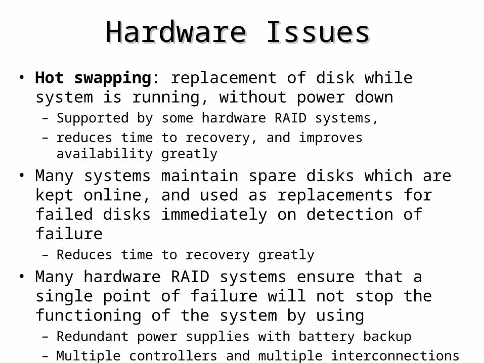
Hardware IssuesHardware Issues• Hot swapping: replacement of disk while system is running,

without power down– Supported by some hardware RAID systems,

– reduces time to recovery, and improves availability greatly

• Many systems maintain spare disks which are kept online, and used as replacements for failed disks immediately on detection of failure– Reduces time to recovery greatly

• Many hardware RAID systems ensure that a single point of failure will not stop the functioning of the system by using – Redundant power supplies with battery backup

– Multiple controllers and multiple interconnections to guard against controller/interconnection failures

Optical DisksOptical Disks• Compact disk-read only memory (CD-ROM)

– Disks can be loaded into or removed from a drive – High storage capacity (640 MB per disk)– High seek times or about 100 msec (optical read head is heavier and

slower)– Higher latency (3000 RPM) and lower data-transfer rates (3-6 MB/s)

compared to magnetic disks

• Digital Video Disk (DVD) – DVD-5 holds 4.7 GB , and DVD-9 holds 8.5 GB – DVD-10 and DVD-18 are double sided formats with capacities of 9.4 GB

and 17 GB– Other characteristics similar to CD-ROM

• Record once versions (CD-R and DVD-R) are becoming popular– data can only be written once, and cannot be erased.– high capacity and long lifetime; used for archival storage – Multi-write versions (CD-RW, DVD-RW and DVD-RAM) also available

Magnetic TapesMagnetic Tapes• Hold large volumes of data and provide high transfer rates

– Few GB for DAT (Digital Audio Tape) format, 10-40 GB with DLT (Digital Linear Tape) format, 100 GB+ with Ultrium format, and 330 GB with Ampex helical scan format

– Transfer rates from few to 10s of MB/s

• Currently the cheapest storage medium – Tapes are cheap, but cost of drives is very high

• Very slow access time in comparison to magnetic disks and optical disks– limited to sequential access.

– Some formats (Accelis) provide faster seek (10s of seconds) at cost of lower capacity

• Used mainly for backup, for storage of infrequently used information, and as an off-line medium for transferring information from one system to another.

• Tape jukeboxes used for very large capacity storage– (terabyte (1012 bytes) to petabye (1015 bytes)

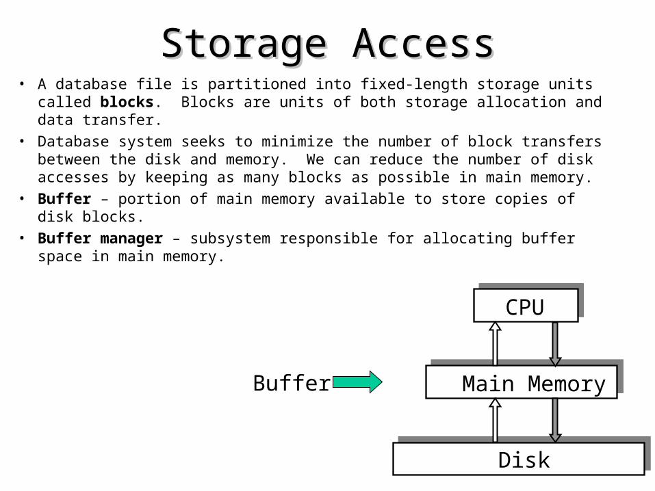
http://www.mdlcorp.com/tapejuke_amle.html

Storage AccessStorage Access• A database file is partitioned into fixed-length storage units called blocks.

Blocks are units of both storage allocation and data transfer.

• Database system seeks to minimize the number of block transfers between the disk and memory. We can reduce the number of disk accesses by keeping as many blocks as possible in main memory.

• Buffer – portion of main memory available to store copies of disk blocks.

• Buffer manager – subsystem responsible for allocating buffer space in main memory.

Buffer

Disk

Main Memory

CPU

Buffer ManagerBuffer Manager

• Programs call on the buffer manager when they need a block from disk.1. If the block is already in the buffer, the requesting

program is given the address of the block in main memory

2. If the block is not in the buffer,1. the buffer manager allocates space in the buffer for the block,

replacing (throwing out) some other block, if required, to make space for the new block.

2. The block that is thrown out is written back to disk only if it was modified since the most recent time that it was written to/fetched from the disk.

3. Once space is allocated in the buffer, the buffer manager reads the block from the disk to the buffer, and passes the address of the block in main memory to requester.

Buffer-Replacement PoliciesBuffer-Replacement Policies• Most operating systems replace the block least recently used

(LRU strategy)• Idea behind LRU – use past pattern of block references as a

predictor of future references• Queries have well-defined access patterns (such as sequential

scans), and a database system can use the information in a user’s query to predict future references– LRU can be a bad strategy for certain access patterns involving

repeated scans of data• e.g. when computing the join of 2 relations r and s by a nested loops

for each tuple tr of r do for each tuple ts of s do if the tuples tr and ts match …

– Mixed strategy with hints on replacement strategy providedby the query optimizer is preferable

Buffer-Replacement Policies (Cont.)Buffer-Replacement Policies (Cont.)• Pinned block – memory block that is not allowed to be

written back to disk.• Toss-immediate strategy – frees the space occupied by a

block as soon as the final tuple of that block has been processed

• Most recently used (MRU) strategy – system must pin the block currently being processed. After the final tuple of that block has been processed, the block is unpinned, and it becomes the most recently used block.

• Buffer manager can use statistical information regarding the probability that a request will reference a particular relation– E.g., the data dictionary is frequently accessed. Heuristic: keep data-

dictionary blocks in main memory buffer

• Buffer managers also support forced output of blocks for the purpose of recovery.

Motivation Motivation

In the beginning of the quarter we talked about data that was organized in a way that is very intuitive to humans, i.e records, attribute, relations etc

The previous slides discussed data from a prospective of the mechanics of hard drives and other mechanical devices.

We need to reconcile the two, so read on…

Page or block is OK when doing I/O, but higher levels of DBMS operate on records, and files of records.

• File: A collection of pages, each containing a collection of records. Must support:

• insert/delete/modify record

• read a particular record (specified using record id, or rid)

• scan all records (possibly with some conditions on the records to be retrieved)

Files of RecordsFiles of Records

Recall a record is another name for a tuple in a relation

name S.S.N street city

Lisa 1272 Blaine Riverside

Bart 5592 Apple Irvine

Files of RecordsFiles of Records

We will consider two possible ways to organize the records on disk

• Heap Files• (Doubly) Linked list• Directory

• Indexes (Indices)

• Simplest file structure contains records in no particular order.

• As file grows and shrinks, disk pages are allocated and de-allocated.

• To support record level operations, we must:

• keep track of the pages in a file

• keep track of free space on pages

• keep track of the records on a page

•There are many alternatives for keeping track of this.

Heap (Unordered) FilesHeap (Unordered) Files

HeaderPage

DataPage

DataPage

DataPage

DataPage

DataPage

DataPage

Pages withFree Space

Full Pages

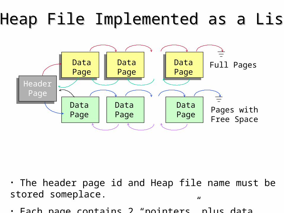
Heap File Implemented as a ListHeap File Implemented as a List

• The header page id and Heap file name must be stored someplace.

• Each page contains 2 “pointers” plus data.

DataPage 1

DataPage 2

DataPage N

HeaderPage

DIRECTORY

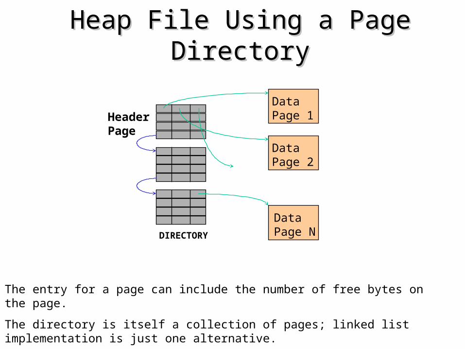
Heap File Using a Page DirectoryHeap File Using a Page Directory

The entry for a page can include the number of free bytes on the page.

The directory is itself a collection of pages; linked list implementation is just one alternative.

Much smaller than linked list of all Heap File pages!

File Organization (Page Formats)File Organization (Page Formats)

• The database is stored as a collection of files. Each file is a collection of records. A record is a sequence of fields.

• One possible approach:– assume record size is fixed

– each file has records of one particular type only

– different files are used for different relations

This case is easiest to implement; will consider variable length records later.

Fixed-Length RecordsFixed-Length Records• We regard a page as being a collection of slots.

• We can view a record’s id (rid) as being a concatenation of the page id, and the slot number.

Slot 1

Slot 2

Slot 3

Slot 4

Page/Block

Information about field types same for all records in a file; stored in system catalogs.

Lisa 1272 Blaine 523

Bart 5592 Apple 44

Marge 7552 11th 34

Slot 1

Slot 2

Slot 3

Slot 4

Bart 5592 Apple 44

Marge 7552 11th 34

Slot 1

Slot 2

Slot 3

Slot 4Marge 7552 11th 34

Bart 5592 Apple 44

Slot 1

Slot 2

Slot 3

Slot 4

Alternative 1:

• Assume that records are stored only in the first N slots.

• When a record is deleted, move the last record in the vacated slot.

Deletion of Fixed-Length RecordsDeletion of Fixed-Length Records

Alternative 2:

• Keep a bitmap which tells us which slots are currently in use.

Deletion of Fixed-Length RecordsDeletion of Fixed-Length Records


Marge 7552 11th 34

Slot 1

Slot 2

Slot 3

Slot 4

1 0 1 0

Variable-Length RecordsVariable-Length Records

• Variable-length records arise in database systems in several ways:– Storage of multiple record types in a file.– Record types that allow variable lengths for one or

more fields.– Record types that allow repeating fields (used in

some older data models).

Variable-Length RecordsVariable-Length Records• Byte string representation

– Attach an end-of-record () control character to the end of each record

– Difficulty with deletion

– Difficulty with growth

4

FieldCount Fields Delimited by Special Symbols

F1 F2 F3 F4


Variable-Length RecordsVariable-Length Records• Array of field offsets

F1 F2 F3 F4

This approach offers direct access to ith field, efficient storage of nulls and small overhead.


We have seen the two techniques for representing variable length records, now lets see how to organize them in a page.

Variable-Length Records: Slotted Page StructureVariable-Length Records: Slotted Page Structure

• Slotted page header contains:– number of record entries– location and size of each record

• Records can be moved around within a page to keep them contiguous with no empty space between them; entry in the header must be updated.

• External pointers should not point directly to record — instead they should point to the entry for the record in header.

Page iRid = (i,N)

Rid = (i,2)

Rid = (i,1)

Pointerto startof freespace

SLOT DIRECTORY

N . . . 2 120 16 24 N

# slots

Can move records on page without changing rid; so, attractive for fixed-length records too.

motivation when we do word processing, graphics, spreadsheets, games etc, we let the operating...

Documents