motions manual sofware
DESCRIPTION
manual of motions sofwareTRANSCRIPT

Maxsurf Motions
Windows Version 19
User Manual
© Bentley Systems, Incorporated 2013


iii
License & Copyright
Maxsurf Motions Program & User Manual
© 2013 Bentley Systems, Incorporated


v
Contents
License & Copyright ........................................................................................................ iii Contents .............................................................................................................................. v About this Manual .............................................................................................................. 1 Chapter 1 Introduction ........................................................................................................ 2
Seakeeping Fundamentals ........................................................................................ 4 Assumptions (Linear Strip Theory) ............................................................... 4 Assumptions (Panel method) ......................................................................... 4 Coordinate System ......................................................................................... 5 Wave Spectra ................................................................................................. 6 Characterising Vessel Response .................................................................... 8 Calculating Vessel Motions ........................................................................... 9 Statistical Measures ....................................................................................... 9 Computational Methods ............................................................................... 10 Visualisation ................................................................................................ 11
Chapter 2 Using Maxsurf Motions ................................................................................... 13 Getting Started ....................................................................................................... 13 Windows Registry .................................................................................................. 13 Opening a Model in Maxsurf Motions ................................................................... 13 Opening the Maxsurf Design File in Maxsurf Motions ......................................... 14 Opening Maxsurf Motions Data ............................................................................. 14 Choosing Analysis Method .................................................................................... 14
Strip theory workflow .................................................................................. 15 Panel method workflow ............................................................................... 15 User input RAO workflow ........................................................................... 15
Measure Hull (Strip theory) ................................................................................... 16 Higher order conformal mappings (Strip theory) ................................................... 17 Mesh Hull (Panel method) ..................................................................................... 18 Additional Hull Parameters (Strip theory) ............................................................. 19
Setting the vessel Type (Strip theory) .......................................................... 20 Setting Mass Distribution (Strip theory and panel method) ........................ 21 Setting Damping Factors (Strip theory) ....................................................... 22
Specifying Remote Locations ................................................................................ 23 Environmental Parameters ..................................................................................... 25 Setting Vessel Speeds, Headings and Spectra ........................................................ 25 Setting the Frequency Range ................................................................................. 27 Completing the Analysis ........................................................................................ 27
Strip theory method ..................................................................................... 27 Calculation of Mapped Sections (strip theory) ...................................................... 29
Solving Seakeeping Analysis ....................................................................... 30 Viewing the Results ............................................................................................... 31
Summary Table Results ............................................................................... 31 MSI – ISO 2631/3 1985 and BS 6841:1987 Results ................................... 33 CG RAO Results .......................................................................................... 34 CG Spectrum Results ................................................................................... 34 Remote Location Spectrum Results ............................................................. 34 Global Hydrodynamic coefficients .............................................................. 35 Sectional Hydrodynamic Coefficient Results (Strip theory) ....................... 36 Panel Pressures ............................................................................................ 36 Drift Forces .................................................................................................. 37 Wave Excitation Forces ............................................................................... 37 Added Mass and Damping ........................................................................... 37

vi
Graphing the Results .............................................................................................. 38 Polar Plots .................................................................................................... 40
Rendered view ........................................................................................................ 41 Calculate Wave Surface ............................................................................... 41 Static (flat) free surface ................................................................................ 42 Roll decay simulation .................................................................................. 43 Regular wave surface ................................................................................... 44 Irregular wave surface ................................................................................. 45 Wavy surface display ................................................................................... 46 Time Simulation and Animation .................................................................. 47 Vessel heading, speed and wave spectrum .................................................. 48
Saving the Maxsurf Motions Model ...................................................................... 49 Saving the Seakeeping Analysis Results ..................................................... 49
Limitations and Guidelines (Strip theory) .............................................................. 50 Underlying Assumptions ............................................................................. 50 Asymmetrical sections ................................................................................. 51 Vessel Speed ................................................................................................ 52 Wave Heading .............................................................................................. 52
Chapter 3 Maxsurf Motions Reference ............................................................................ 53 Windows ................................................................................................................ 53
Inputs Window ............................................................................................. 53 Results Window ........................................................................................... 53 Graph Window ............................................................................................. 54 Polar Window .............................................................................................. 55
Toolbars ................................................................................................................. 55 File Toolbar.................................................................................................. 55 View Toolbar ............................................................................................... 55 Analysis Toolbar .......................................................................................... 56 Contour Toolbar ........................................................................................... 56 Window Toolbar .......................................................................................... 56 Results Toolbar ............................................................................................ 56 Graph window Toolbar ................................................................................ 56
Menus ..................................................................................................................... 56 File Menu ..................................................................................................... 57 Edit Menu .................................................................................................... 58 View Menu .................................................................................................. 59 Analysis Menu ............................................................................................. 60 Display Menu ............................................................................................... 61 Data Menu.................................................................................................... 62 Window Menu ............................................................................................. 63 Help Menu ................................................................................................... 63
Chapter 4 Theoretical Reference ...................................................................................... 65 Seakeeping Theory ................................................................................................. 66
Wave Spectra Theory ................................................................................... 67 What the Vessel Sees ................................................................................... 72 Characterising Vessel Response .................................................................. 73 Calculating Vessel Motions ......................................................................... 76 Absolute Vessel Motions ............................................................................. 77 Statistical Measures ..................................................................................... 78 Probability Measures ................................................................................... 80 Calculation of Subjective Magnitude and Motion Sickness Incidence ........ 81 Speed Loss ................................................................................................... 84
Glossary ................................................................................................................. 86
vii
Nomenclature ......................................................................................................... 86 Bibliography and References ................................................................................. 88
Appendix A Strip Theory Formulation ............................................................................ 91 Calculation of coupled heave and pitch motions ................................................... 91
Heave and Pitch Motion of a Vessel in a Seaway........................................ 92 Solution of Coupled Heave and Pitch Motions ............................................ 93 Global Added Mass and Damping (Strip Theory) ....................................... 93 Wave Excitation Force and Moment ........................................................... 95 Arbitrary Wave Heading .............................................................................. 95 Diffraction Force .......................................................................................... 96 Froude-Krilov Force .................................................................................... 97 Head Seas Approximation ........................................................................... 97 Salvesen et al. (1970) Approximation ......................................................... 98 Wave Attenuation (Smith Effect) ................................................................ 98 Added Resistance of a Vessel in a Seaway .................................................. 98 2D Ship Sections ........................................................................................ 100 Calculation of Added Mass and Damping of 2D Ship Sections ................ 100 Calculation of multipole expansion coefficients ........................................ 100 Least squares solution to over-defined set of linear equations .................. 101 Calculation and integration of pressure functions around contour ............ 102 Evaluation of hydrodynamic coefficients .................................................. 103 Checking the solution ................................................................................ 103 Important notes .......................................................................................... 103 Added Mass at Infinite Frequency ............................................................. 103 Non-Dimensional Damping Coefficient .................................................... 103 Non-Dimensional Added Mass .................................................................. 104 Non-Dimensional Frequency ..................................................................... 104 Representation of Ship-Like Sections by Conformal Mapping ................. 104 Derivative of Conformal Mapping............................................................. 106 Shear Force and Bending Moment due to Ship Motion in a Seaway ........ 106 Inertial Component .................................................................................... 107 Hydrostatic (Restoring) Component .......................................................... 107 Wave Excitation Component ..................................................................... 108 Hydrodynamic Component ........................................................................ 109
Calculation of uncoupled roll motion................................................................... 109 Equation of motion for roll ........................................................................ 110
Appendix B Strip theory validation ................................................................................ 115 Maxsurf Motions Validation 1 – NPL Round Bilge series .................................. 115
Introduction ................................................................................................ 115 Analysis Procedure .................................................................................... 116 Results ........................................................................................................ 116 Slow Speed ................................................................................................ 116 Moderate Speed ......................................................................................... 117 High Speed ................................................................................................. 117 Conclusions ................................................................................................ 117 References .................................................................................................. 118 Figures ....................................................................................................... 118
Maxsurf Motions Validation 2 – Series 60 .......................................................... 136 Introduction ................................................................................................ 136 Hullform principal particulars.................................................................... 137 Analysis Procedure .................................................................................... 137 Results ........................................................................................................ 137 Conclusions ................................................................................................ 138
viii
References .................................................................................................. 138 Figures ....................................................................................................... 138
Maxsurf Motions Validation 3 – SA van der Stel ................................................ 140 Hullform and test conditions ...................................................................... 140 Results ........................................................................................................ 142 Conclusions ................................................................................................ 146 Bibliography .............................................................................................. 146
Appendix C Panel Method Formulation ......................................................................... 148 LINEAR POTENTIAL THEORY ....................................................................... 148
Coordinates and Boundary Value Problem ................................................ 148 Boundary Integral Equation ....................................................................... 149 Equations of Motion .................................................................................. 149 Mean Drift Forces and Moments ............................................................... 150
Appendix D Panel Method Validation ........................................................................... 151 Validation with experiment .................................................................................. 151 Verification against WAMIT ............................................................................... 155
Motions ...................................................................................................... 155 Wave forces ............................................................................................... 156 Added Mass ............................................................................................... 157 Damping..................................................................................................... 158 Drift Forces ................................................................................................ 159
Verification against AQWA ................................................................................. 160 Index ............................................................................................................................... 164

About this Manual
Page 1
About this Manual
This manual describes Maxsurf Motions, an application which may be used to predict
the motion and seakeeping performance of vessels designed using Maxsurf. This manual
is organised into the following chapters:
Chapter 1 Introduction
Contains a description of Maxsurf Motions, its principal features and mode of operation.
Chapter 2 Using Maxsurf Motions
Explains how to use Maxsurf Motions and provides step-by-step examples to guide the
user through the operation of the program.
Chapter 3 Maxsurf Motions Reference
Gives details of each of Maxsurf Motions's menu commands and provides a more
detailed guide to the calculation methods and strip theory algorithm used in Maxsurf
Motions.
Chapter 4 Theoretical Reference
Gives a summary of the theoretical background to Maxsurf Motions.
Appendix A Strip Theory Formulation
Presents more in depth explanation of the theoretical model used in Maxsurf Motions.
Appendix B Strip theory validation
Gives details of some of the validation work carried out with Maxsurf Motions.

Chapter 1 Introduction
2
Chapter 1 Introduction
Maxsurf Motions is the seakeeping analysis program in the Maxsurf software suite. It
uses the Maxsurf geometry file to calculate the response of the vessel to user-defined sea
conditions. Two methods are available to calculate the vessels response: a linear strip
theory method and a panel method. The panel method option is only available in Maxsurf
Motions Advanced.
The linear strip theory method is based on the work of Salvesen et al, it is used to
calculate the coupled heave and pitch response of the vessel. The roll response is
calculated using linear roll damping theory. In addition to graphical and tabular output of
numerical results data, Maxsurf Motions is also able to provide an animation of the
vessel’s response to specified sea conditions.
The panel method is a first-order diffraction/radiation hydrodynamic analysis in which a
constant panel based boundary element method (BEM) is used. The panel method
generates its analysis elements based on the geometry from the NURBS surfaces in the
Maxsurf design file. The panel method generates Response Amplitude Operators
(RAOs) for all six degrees of freedom: surge, sway, heave, roll, pitch and yaw. The
panel method is valid for a very large range of geometries but is restricted to zero
forward speed. In addition to outputting RAOs, the panel method output also includes
hydrodynamic added mass and damping, first order wave exciting forces and moments,
mean drift forces and moments and pressure on the vessel wetted surface.
Strip theory along with the Panel method, and hence Maxsurf Motions, is able to provide
reasonably accurate seakeeping predictions for a wide range of vessel types. The speed of
the analysis and its integration into the rest of the Maxsurf suite, make Maxsurf Motions
particularly useful in initial design stage. For a greater insight into the accuracy that can
be achieved by Maxsurf Motions, please refer to the validation appendices at the end of
this manual.

Chapter 1 Introduction
Page 3
Maxsurf Motions workflow
Continue to read: Seakeeping Fundamentals on page 4.

Chapter 1 Introduction
4
Seakeeping Fundamentals
In this section we will outline some of the fundamental principles used in seakeeping
analysis.
Assumptions
Coordinate System
Wave Spectra
Characterising Vessel Response
Calculating Vessel Motions
Statistical Measures
Computational Methods
Visualisation
Users familiar with these concepts may wish to go straight to Chapter 2 Using Maxsurf
Motions.
Assumptions (Linear Strip Theory)
When linear strip theory is used to compute the coupled heave and pitch motions of the
vessel, the following underlying assumptions are implied:
Slender ship: Length is much greater than beam or draft and beam is much less
than the wavelength).
Hull is rigid.
Speed is moderate with no lift from forward speed.
Motions are small and linear with respect to wave amplitude.
Hull sections are wall-sided.
Water depth is much greater than wavelength so that deep-water wave
approximations may be applied.
The hull has no effect on the incident waves (so called Froude-Kriloff hypothesis).
A simplified forced, damped mass-spring system is assumed for the uncoupled roll
motions. This assumes the following
An added inertia in roll is used which is assumed to be a constant proportion of the
roll inertia.
A constant user-specified linear damping is used.
Please see Appendix A for further details on the strip theory formulation for coupled
heave and pitch and the simplified method used for roll.
Assumptions (Panel method)
The usual linear potential theory assumptions apply:

Chapter 1 Introduction
Page 5
Wave height and steepness are assumed to be small so that linear wave theory
may be used.
Fluid is assumed to be inviscid and incompressible.
Fluid flow is assumed to be irrotational.
Coordinate System
The coordinate system used by Maxsurf Motions is the same as for Maxsurf. The
coordinate system has the origin at the user defined zero point.
Maxsurf Motions User Coordinate System and view Windows are the same as for Maxsurf
X-axis +ve forward -ve aft
Y-axis +ve starboard -ve port
Z-axis +ve up -ve down
When calculating motions at remote locations, the vessel is assumed to rotate about the
centre of gravity. Hence the distance of the remote location from the centre of gravity is
of interest. Maxsurf Motions calculates this distance internally and all positions are
measured in the coordinate system described above.
A vessel has six degrees of freedom, three linear and three angular. These are: surge,
sway, heave (linear motions in x, y, z axes respectively) and roll, pitch, yaw (angular
motions about the x, y, z axes respectively). For convenience, the degrees of freedom are
often given the subscripts 1 to 6; thus heave motion would have a subscript 3 and pitch 5.
Wave direction is measured relative to the vessel track and is given the symbol . Thus following waves are at
= 0; starboard beam seas are 90; head seas 180 and port beam seas 270.
Chapter 1 Introduction
6
Wave Spectra
Irregular ocean waves are often characterised by a "wave spectrum", this describes the
distribution of wave energy (height) with frequency.
Characterisation
Ocean waves are often characterised by statistical analysis of the time history of the
irregular waves. Typical parameters used to classify irregular wave spectra are listed
below:
Characterisation of irregular wave time history
mean of many wave amplitude measurements
mean of many wave height measurements
mean of many wave period measurements between successive peaks
mean of many wave period measurements between successive troughs
mean of many wave period measurements between successive zero up-
crossings
mean of many wave period measurements between successive zero down-
crossings
mean of many wave period
modal wave period
mean of highest third amplitudes or significant amplitude
mean of highest third wave heights or significant wave height
variance of the surface elevation relative to the mean (mean square)
standard deviation of surface elevation to the mean (root mean square)
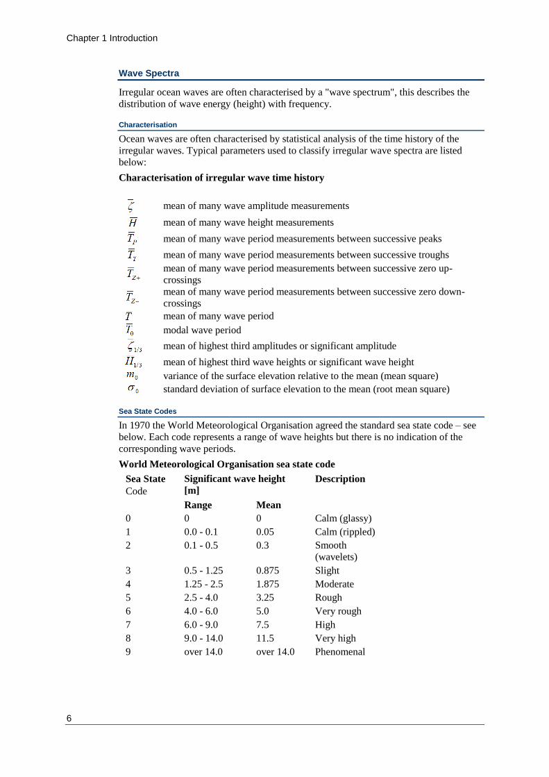
Sea State Codes
In 1970 the World Meteorological Organisation agreed the standard sea state code – see
below. Each code represents a range of wave heights but there is no indication of the
corresponding wave periods.
World Meteorological Organisation sea state code
Sea State
Code
Significant wave height
[m] Description
Range Mean
0 0 0 Calm (glassy)
1 0.0 - 0.1 0.05 Calm (rippled)
2 0.1 - 0.5 0.3 Smooth
(wavelets)
3 0.5 - 1.25 0.875 Slight
4 1.25 - 2.5 1.875 Moderate
5 2.5 - 4.0 3.25 Rough
6 4.0 - 6.0 5.0 Very rough
7 6.0 - 9.0 7.5 High
8 9.0 - 14.0 11.5 Very high
9 over 14.0 over 14.0 Phenomenal
Chapter 1 Introduction
Page 7
Sea state data may also be obtained for specific sea areas and times of year. This can be
useful routing information. One of the best sources of this information is Hogben and
Lumb (1967).
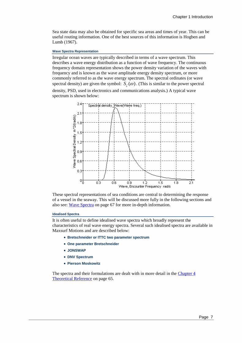
Wave Spectra Representation
Irregular ocean waves are typically described in terms of a wave spectrum. This
describes a wave energy distribution as a function of wave frequency. The continuous
frequency domain representation shows the power density variation of the waves with
frequency and is known as the wave amplitude energy density spectrum, or more
commonly referred to as the wave energy spectrum. The spectral ordinates (or wave
spectral density) are given the symbol: S ( ) . (This is similar to the power spectral
density, PSD, used in electronics and communications analysis.) A typical wave
spectrum is shown below:
These spectral representations of sea conditions are central to determining the response
of a vessel in the seaway. This will be discussed more fully in the following sections and
also see: Wave Spectra on page 67 for more in-depth information.
Idealised Spectra
It is often useful to define idealised wave spectra which broadly represent the
characteristics of real wave energy spectra. Several such idealised spectra are available in
Maxsurf Motions and are described below:
Bretschneider or ITTC two parameter spectrum
One parameter Bretschneider
JONSWAP
DNV Spectrum
Pierson Moskowitz
The spectra and their formulations are dealt with in more detail in the Chapter 4
Theoretical Reference on page 65.

Chapter 1 Introduction
8
Encounter Spectrum
An important concept when calculating vessel motions is that of the encountered wave
spectrum. This is a transformation of the wave spectrum which describes the waves
encountered by a vessel travelling through the ocean at a certain speed. This is
effectively a Doppler shift of the spectrum which smears the spectrum towards the higher
frequencies in head seas and towards the lower frequency in following seas.
A full explanation of this effect is given in Chapter 4 Theoretical Reference, section
What the Vessel Sees on page 71.
Characterising Vessel Response
This section outlines the method used to describe a vessel's response in a seaway.
Harmonic Response of Damped, Spring, Mass system
For most purposes, it is sufficient to model the vessel as a set of coupled spring, mass,
damper systems undergoing simple harmonic motion. This is assumed by Maxsurf
Motions and most other seakeeping prediction methods. This method may be
successfully applied to the analysis of the vessel's motions provided that these motions
are linear and that the principle of superposition holds. These assumptions are valid
provided that the vessel is not experiencing extremely severe conditions.
Response Amplitude Operator
The Response Amplitude Operator (RAO), also referred to as a transfer function (this is
similar to the response curve of an electronic filter), describes how the response of the
vessel varies with frequency. These are normally non-dimensionalised with wave height
or wave slope. Typical heave and pitch RAOs are shown below:
It may be seen that the RAOs tend to unity at low frequency, this is where the vessel
simply moves up and down with the wave and acts like a cork. At high frequency, the
response tends to zero since the effect of many very short waves cancel out over the
length of the vessel. Typically the vessel will also have a peak of greater than unity; this
occurs close to the vessels natural period. The peak is due to resonance. An RAO value
of greater than unity indicates that the vessel's response is greater than the wave
amplitude (or slope).

Chapter 1 Introduction
Page 9
Calculating Vessel Motions
Assuming linearity, the vessel's RAOs depend only on the vessel's geometry, speed and
heading. Thus once the RAOs have been calculated the motion of a vessel in a particular
sea state of interest may be calculated.
It is hence possible to obtain a spectrum for a particular vessel motion in a particular sea
spectrum:
See Chapter 4 Theoretical Reference on page 65 for further details on how these
calculations are performed.
Statistical Measures
Often it is important to know certain statistical measures of the motion spectrum. These
can be used to determine significant motions, Root Mean Square (RMS) motions as well
as other measures such as Motion Sickness Incidence (MSI).
It is also possible to calculate the probability of exceeding certain limiting criteria, such
as limiting maximum vertical accelerations, propeller emergence, slamming and so forth.
Maxsurf Motions is able to calculate the significant and RMS motions, velocities and
accelerations of the heave, pitch and roll motions at the centre of gravity of the vessel. In
addition, the user is able to specify remote locations away from the centre of gravity.
Maxsurf Motions calculates the vertical absolute and relative motions as well as the MSI
at these locations.
For further information please refer to Statistical Measures and Probability Measures on
pages 78 and 80.

Chapter 1 Introduction
10
Computational Methods
Several numerical methods are available for estimating a vessel's response. Two of the
most widely used are Strip Theory and Panel Methods. Maxsurf Motions uses linear strip
theory method to predict the vessels heave and pitch response. Roll response is estimated
assuming that the vessel behaves as a simple, damped, spring/mass system, and that the
added inertia and damping are constant with frequency. The linear strip theory method,
originally developed in the 1970s (Salvesen et al. 1970) is useful for many applications;
unlike more advanced methods, it is relatively simple to use and not too computationally
intense.
The panel method is used when looking at vessel motions in all six degrees of freedom at
zero forward speed and is applicable to a wider range of vessel geometries than linear
strip theory. Maxsurf Motions uses a 3d first order diffraction/radiation hydrodynamics
solver.
Strip Theory
Strip theory is a frequency-domain method. This means that the problem is formulated as
a function of frequency. This has many advantages, the main one being that
computations are sped up considerably. However, the method, generally becomes limited
to computing the linear vessel response.
The vessel is split into a number of transverse sections. Each of these sections is then
treated as a two-dimensional section in order to compute its hydrodynamic
characteristics. The coefficients for the sections are then integrated along the length of
the hull to obtain the global coefficients of the equations of motion of the whole vessel.
Finally the coupled equations of motion are solved.
Further details of Maxsurf Motions's implementation of the Strip Theory method is given
in the Appendix A Strip Theory Formulation on page 91.
Conformal Mapping
Fundamental to strip theory is the calculation of the sections' hydrodynamic properties.
There are two commonly used methods: conformal mapping and the Frank Close Fit
method. The former is used by Maxsurf Motions and will be discussed at greater length.
Conformal mappings are transformations which map arbitrary shapes in one plane to
circles in another plane. One of the most useful is the Lewis mapping. This maps a
surprising wide range of ship-like sections to the unit circle, and it is this method that is
used by Maxsurf Motions. Lewis mappings use three parameters in the conformal
mapping equation, but by adding more parameters, it is possible to map an even wider
range of sections. See: Calculation of Mapped Sections on page 29 for more information.
Panel Method
The Maxsurf Motions Panel Method is a low speed radiation/diffraction solver in the
frequency domain. It performs linear analysis of the interaction of surface waves with
floating structures. The body is defined by a mesh auto generated on the NURBS surface
in the Maxsurf design file (.msd). The mesh size and shape can be controlled by user
specified input parameters. The solutions of the velocity potential and source strength
are assumed constant over each panel.

Chapter 1 Introduction
Page 11
The panel method is also is a frequency-domain method. This means that the problem is
formulated as a function of frequency. This has many advantages, the main one being
that computations are sped up considerably.
Further details of Maxsurf Motions's implementation of the Panel method are given in
Appendix C Panel Method Formulation on page 148.
Visualisation
Maxsurf Motions is able to provide a three dimensional view of the vessel in the waves.
This can be either a static image or an animation of the vessel travelling through the
waves.
Further details are given in:
Roll decay simulation on page 43
Time Simulation and Animation on page 47


Chapter 2 Using Seakeeper
Page 13
Chapter 2 Using Maxsurf Motions
You have been introduced to the way in which Maxsurf Motions works and can now go
on to learn in detail how to use Maxsurf Motions by following the examples outlined in
this chapter.
Getting Started
Opening a Model in Maxsurf Motions
Additional Hull Parameters
Environmental Parameters
Completing the Analysis
Viewing the Results
Panel Pressures
The panel pressures table displays the panel pressure values for the selected
frequency. By default values for all the panels are displayed, alternatively the user
can specify just to see just the results for the panel of interest (select from the drop
down list on the results toolbar).
The magnitude and phase of the pressure are shown. In addition the magnitude of the
Incident, Diffraction and Radiation components of the pressure are shown. The non-
dimensional values are displayed. The pressure values are non-dimensionalised
according to the water density (ρ), gravity(g) and wave amplitude (A):
Pressure’=Pressure/ρgA
Drift Forces
Drift forces and moments are displayed in the Drift Forces table. Each row representing
the value for a single frequency and heading. The values displayed are non-dimensional.
Drift forces (surge, sway and heave) are non-dimensionalised according to water density
(ρ), gravity(g), characteristic length (L) and wave amplitude (A):
Drift force’=Drift force/ρgLA2
Drift moments (roll, pitch and yaw) are non-dimensionalised according to water density
(ρ), gravity(g), characteristic length (L) and wave amplitude (A):
Drift moment’=Drift moment/ρgL2A
2
Characteristic length defaults to the vessel’s maximum dimension. The characteristic
length can be altered by the user in the Analysis | Mesh Hull… dialog.
Wave Excitation Forces
Wave excitation forces are displayed in the wave excitation forces table. Each row
represents the exciting force in each of the 6 degrees of freedom for a frequency and
heading. The non-dimensional force magnitude and phase are presented for surge, sway,
heave, roll, pitch and yaw respectively.
Wave excitation forces (surge, sway and heave) are non-dimensionalised according to
water density (rho), gravity(g), displaced volume (▽), characteristic length (L) and wave
amplitude (A):

Chapter 2 Using Seakeeper
14
Wave Force’=Wave Force/( ρ g▽A/L)
Wave excitation moments (roll, pitch and yaw) are non-dimensionalised according to
water density (rho), gravity(g), displaced volume (▽) and wave amplitude (A):
Wave Force’=Wave Force/( ρ g▽A)
Characteristic length defaults to the vessel’s maximum dimension. The characteristic
length can be altered by the user in the Analysis | Mesh Hull… dialog.
Added Mass and Damping
Added mass and damping results are displayed in the Added Mass and Damping table of
the results window. The 6x6 Added Mass (Aij) and Damping (Bij) coefficient matricies
are presented for each frequency.
The coefficients are non dimensionalised using water density (ρ), gravity (g), volumetric
displacement (▽), wave amplitude (A), wave frequency(ω) and characteristic length (L).
For the added mass coefficients (Aij) the values are non-dimensionalised as follows:
i=1-3 and j=1-3: Aij’=Aij/( ρ▽)
i=1-3 and j=4-6: Aij’=Aij/( ρ▽L)
i=4-6 and j=1-3: Aij’=Aij/( ρ▽L)
i=4-6 and j=4-6: Aij’=Aij/( ρ▽L2)
For the added mass coefficients (Bij) the values are non-dimensionalised as follows:
i=1-3 and j=1-3: Bij’=Bij/( ρ▽ω)
i=1-3 and j=4-6: Bij’=Bij/( ρ▽L ω)
i=4-6 and j=1-3: Bij’=Bij/( ρ▽L ω)
i=4-6 and j=4-6: Bij’=Bij/( ρ▽L2 ω)
Graphing the Results
Rendered view
Time Simulation and Animation
Saving the Maxsurf Motions Model
Saving the Seakeeping Analysis Results
Limitations and Guidelines
Getting Started
Install Maxsurf Motions from the CD. Maxsurf Motions may then be started, and will
display three windows containing a view of the Maxsurf model, a tabulated results
window and a graph of the results.

Chapter 2 Using Seakeeper
Page 15
Windows Registry
Certain preferences used by the Maxsurf Motions program are stored in the Windows
registry. It is possible for this data to become corrupted, or you may simply want to
revert back to the default configuration. To clear Maxsurf Motions's preferences, start the
program with the Shift key depressed. You will be asked if you wish to clear the
preferences, click OK.
These preferences are:
Colour settings of contours and background
Fonts
Window size and location
Recent files
Units
Opening a Model in Maxsurf Motions
A Maxsurf Motions model consists of Maxsurf surface information and Maxsurf Motions
input data, such as sea environment, speeds etc., and also information on the hull
characteristics such as damping factors and moments of inertia.
Opening the Maxsurf Design File in Maxsurf Motions
Choose Open from the File menu. Select the file titled ‘Maxsurf Motions Sample.msd’ in
the ‘Maxsurf\Sample Designs’ folder and open it. This file contains the Maxsurf surface
information of a simple Maxsurf design.
Note:
The .msd file contains the Maxsurf surface information.
Opening Maxsurf Motions Data
Existing Maxsurf Motions designs have Maxsurf Motions input data already defined and
saved in a .skd file. To open existing Maxsurf Motions data, choose “Open Maxsurf
Motions Data” from the File menu. Sample Seakeeping data corresponding to the
Maxsurf Motions Sample.msd file can be found in the Sample Designs folder: Maxsurf
Motions Sample.skd.
The Maxsurf Motions data consists of:
1) Input data window data
Locations, Speeds, Headings and Spectra
2) Analysis menu data
Measured Hull sections, Vessel type, Mass distribution, Damping factors,
Frequency range, Environment, Analysis methods.
Note:
The .skd file contains all Maxsurf Motions analysis input data.

Chapter 2 Using Seakeeper
16
Choosing Analysis Method
Depending on the required output the user needs to specify the type of analysis method to
be used. An overview of the applicability and limitations of each method are given
below:
method Speed range (Fn) Motions analysed Applicable vessels
Strip theory 0.0 ~ 0.7 Heave, roll, pitch “slender”
Panel method 0.0 ~ 0.1 Surge, sway, heave,
Roll, pitch, yaw
all
The analysis method is chosen by selecting from the Analysis | Analysis Type menu:
Depending on which analysis method is chosen a different analysis workflow will be
required. As a general rule, once the analysis type has been selected the user should
sequentially work through the other input dialogs as listed in the Analysis menu (enter
data only in the commands that are enabled).
Strip theory workflow
The following steps must be taken to perform a strip theory analysis (more detailed
information on each of the steps is provided in subsequent sections). Each command is
accessed from the Analysis menu:
Select “Strip Theory” from the “Analysis Type” list.
Select “Measure Hull…” to define the parameters for the conformal mapping.
Select “Specify Vessel Type…” to define the number of hulls of the vessel
Select “Mass distribution…” to define the gyradii and VCG of the vessel.
Select “Damping Factors…” to define the non dimensional heave, pitch and roll
damping factors.
Select “Environment…” to specify the water density.
Select “Frequency Range…” to define the number of frequencies at which to
calculate the RAOs.
Select “Strip theory method…” to specify the Transom Terms, Added Resistance
and Wave Force methods to be used during the strip theory calculations.
Once the analysis specific settings have been entered the user needs to set the spectral
analysis settings. These include the vessel speeds, vessel headings, wave spectrums and
locations at which motions are to be evaluated (remote locations). These values are to be
entered in the Windows | Inputs windows. As a minimum 1 speed, 1 heading and 1 wave
spectrum must be entered. Once the minimum required inputs have been specified the
Analysis | Solve Seakeeping Analysis function will become enabled.

Chapter 2 Using Seakeeper
Page 17
Panel method workflow
The following steps must be taken to perform a Panel Method analysis (more detailed
information on each of the steps is provided in subsequent sections). Each command is
accessed from the Analysis menu:
Select “Panel Method” from the “Analysis Type” list.
Select “Mesh Hull” to define the parameters for meshing the surfaces and to
execute the automated meshing process.
Select “Mass distribution” to define the gyradii and VCG of the vessel.
Select “Environment…” to specify the water density.
Select “Frequency Range” to define the number of frequencies at which to
calculate the RAOs.
Once the analysis specific settings have been entered the user needs to set the spectral
analysis settings. These include the vessel headings, wave spectrums and locations at
which motions are to be evaluated (remote locations). These values are to be entered in
the Windows | Inputs windows. As a minimum 1 heading and 1 wave spectrum must be
entered. Once the minimum required inputs have been specified the Analysis | Solve
Seakeeping Analysis function will become enabled.
User input RAO workflow
Alternatively the user may wish to perform a spectral analysis on a set of RAO data that
has been calculated/supplied from a 3rd
party. In this case the user just needs to open the
RAO text file using the File | Import | RAO Text… command. Set the analysis type to
“User Input RAOS” and specify the spectral analysis parameters (speeds, headings, wave
spectrums and locations) to perform the seakeeping analysis. The text file format takes
the following form:
RAO text file from Maxsurf Motions. 12 October 2012 15:33:05
Heading = 180.000 deg Speed = 0.000 kts
15.7080 180 1 0.9522 89.358 0.0107 0.9521
…
Line 1 – comment
Line 2 – specify the heading in degrees and the speed in kts
Line 3 onwards – RAO data points. Period (sec), heading (deg), mode (1=surge, 2=
sway etc), RAO (Mag), RAO (phase deg), RAO (Real), RAO (Imag.)
Measure Hull (Strip theory)
Choose Analysis | Measure Hull from the menu. By default all the surfaces will be
measured and 11 equally spaced sections will be calculated. This is sufficient for initial
calculations but for more accurate predictions, the number of sections should be
increased to between 15 and 30.
If the design includes surfaces which are trimmed, then the Trim Surfaces checkbox
should be ticked.

Chapter 2 Using Seakeeper
18
By default sections are mapped with Lewis sections (see Calculation of Mapped Sections
on page 29 for further details).. This has the limitation that, for sections which are very
wide and/or deep and have a low section area, the mapping may be inaccurate. This may
occur for sections which have a skeg, rudder or keel. For sections such as these, it may
be necessary to remove the skeg, rudder or keel surfaces from those that are measured.
For heave and pitch motions, removing these surfaces is unlikely to have a significant
influence on the results. Roll motions use the damping factor specified by the user, which
should include the effect of such appendages (see Setting Damping Factors section on
page 22).
Maxsurf Motions will automatically choose the best Lewis section that can be fitted to
the section. If the sectional area coefficient is too low for the section’s depth, Maxsurf
Motions will limit the draft of the mapping. Conversely, if the sectional area coefficient
is too large, Maxsurf Motions will select the Lewis section with the largest possible
sectional area coefficient for the given section breadth to draft ratio.
However, in most circumstances, it is normally advisable to remove appendages from the
design, this will result in better modelling of the main hull. It should also be noted that a
feature of the conformal mapping is that the mapped section is always vertical where it
crosses the horizontal axis and horizontal where it crosses the vertical axis. However, this
is not generally a major limitation.
Chapter 2 Using Seakeeper
Page 19
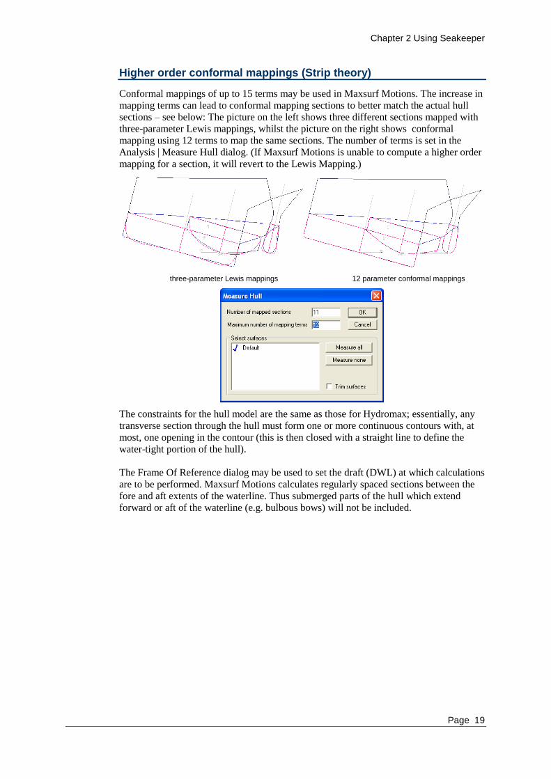
Higher order conformal mappings (Strip theory)
Conformal mappings of up to 15 terms may be used in Maxsurf Motions. The increase in
mapping terms can lead to conformal mapping sections to better match the actual hull
sections – see below: The picture on the left shows three different sections mapped with
three-parameter Lewis mappings, whilst the picture on the right shows conformal
mapping using 12 terms to map the same sections. The number of terms is set in the
Analysis | Measure Hull dialog. (If Maxsurf Motions is unable to compute a higher order
mapping for a section, it will revert to the Lewis Mapping.)
three-parameter Lewis mappings 12 parameter conformal mappings
The constraints for the hull model are the same as those for Hydromax; essentially, any
transverse section through the hull must form one or more continuous contours with, at
most, one opening in the contour (this is then closed with a straight line to define the
water-tight portion of the hull).
The Frame Of Reference dialog may be used to set the draft (DWL) at which calculations
are to be performed. Maxsurf Motions calculates regularly spaced sections between the
fore and aft extents of the waterline. Thus submerged parts of the hull which extend
forward or aft of the waterline (e.g. bulbous bows) will not be included.

Chapter 2 Using Seakeeper
20
The Lewis mappings are calculated from the section’s properties: draft, waterline beam
and cross-sectional area. In some cases the Lewis mapping will be a poor fit to the
section, this will occur if: the waterline beam is very narrow for the depth and area (e.g.
near a bulbous bow or swath hull); there are multiple contours (e.g. bulbous bow or keel
bulb) or where the hull sections are asymmetrical. In this last case, Maxsurf Motions will
compute a symmetrical Lewis section having the draft, waterline beam and cross-
sectional area of the asymmetrical section.
Occasionally Maxsurf Motions may have problems forming sections at the extremities of
the hull; this can happen particularly if there is, say, a very slight wobble in a vertical
transom. If this occurs, the following error message will be displayed.
The problem can normally be solved by ensuring that a section can be formed; either by
moving the perpendiculars slightly or by adjusting the models surfaces in Maxsurf.
Mesh Hull (Panel method)
Choose Analysis | Mesh Hull from menu. This menu option will only be enabled with the
analysis type is set to Panel Method. The mesh hull dialog will appear:

Chapter 2 Using Seakeeper
Page 21
The user has control over the following parameters:
Mesh - specifies whether the surface is to be automeshed
Min. edge length – specifies the user recommended minimum edge length of triangles in
the final mesh.
Max. edge length – specifies the user recommended maximum edge length of triangles
in the final mesh.
Node merge tolerance – a relative tolerance that dictates whether or not two nodes are so
close that they should be merged. The value should lie between 0.001 and 0.05. The
user will be warned if they try to enter a value outside this range.
Geometric tolerance - A relative tolerance that specifies how far a tri edge can lie off the
surface with which it is associated. The value should lie between 0.001 and 0.05. The
user will be warned if they try to enter a value outside this range. A lower value will
create smaller triangles in areas of high surface curvature.
Once the OK button is hit to close the dialog the mesh will be generated on the surface.
The mesh visibility will be automatically turned on after a mesh generation. Use the
“analysis contours” button
The hull mesh will be saved in the seakeeper data file (*.skd). Alternatively a mesh can
be saved to and loaded from an STL file. STL is a universally recognized trimesh file
format.
If for some reason the user wanted to manipulate the mesh after it has been automatically
generated by the application then this can be done. Firstly save the *.stl file (File |
Export | STL mesh). Open the stl file in 3rd
party software (or simply in a text editor) and
manipulate the verticies until the desired shape is achieved), resave and import back into
Maxsurf Motions (File | Import | STL Mesh). Alternatively if the user wanted to bypass
the Automatic mesh generator in Maxsurf Motions all together then an STL file from
another application may be imported directly.
Additional Hull Parameters (Strip theory)
A number of other hull parameters are required by Maxsurf Motions, these are reviewed
in the following text:
Chapter 2 Using Seakeeper
22
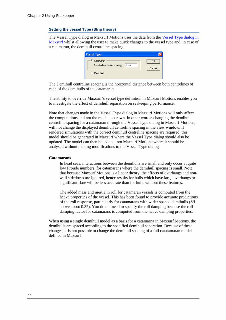
Setting the vessel Type (Strip theory)
The Vessel Type dialog in Maxsurf Motions uses the data from the Vessel Type dialog in
Maxsurf whilst allowing the user to make quick changes to the vessel type and, in case of
a catamaran, the demihull centreline spacing:
The Demihull centreline spacing is the horizontal distance between both centrelines of
each of the demihulls of the catamaran.
The ability to override Maxsurf’s vessel type definition in Maxsurf Motions enables you
to investigate the effect of demihull separation on seakeeping performance.
Note that changes made in the Vessel Type dialog in Maxsurf Motions will only affect
the computations and not the model as drawn. In other words: changing the demihull
centreline spacing for a catamaran through the Vessel Type dialog in Maxsurf Motions,
will not change the displayed demihull centreline spacing in the view window. If
rendered simulations with the correct demihull centreline spacing are required, this
model should be generated in Maxsurf where the Vessel Type dialog should also be
updated. The model can then be loaded into Maxsurf Motions where it should be
analysed without making modifications to the Vessel Type dialog.
Catamarans
In head seas, interactions between the demihulls are small and only occur at quite
low Froude numbers, for catamarans where the demihull spacing is small. Note
that because Maxsurf Motions is a linear theory, the effects of overhangs and non-
wall sidedness are ignored, hence results for hulls which have large overhangs or
significant flare will be less accurate than for hulls without these features.
The added mass and inertia in roll for catamaran vessels is computed from the
heave properties of the vessel. This has been found to provide accurate predictions
of the roll response, particularly for catamarans with wider spaced demihulls (S/L
above about 0.35). You do not need to specify the roll damping because the roll
damping factor for catamarans is computed from the heave damping properties.
When using a single demihull model as a basis for a catamarna in Maxsurf Motions, the
demihulls are spaced according to the specified demihull separation. Because of these
changes, it is not possible to change the demihull spacing of a full catatamaran model
defined in Maxsurf

Chapter 2 Using Seakeeper
Page 23
In addition, the demihull spacing is also given in the Summary results table
Maxsurf Motions catamaran modelled as a single demihull in Maxsurf
Also see:
Asymmetrical sections on page 51.
Setting Mass Distribution (Strip theory and panel method)
Maxsurf Motions requires the pitch and roll inertias of the vessel. These are input as
gyradii in percent of overall length and beam respectively. Typical values are pitch
gyradius 25%; roll gyradius 35%–40%. The gyradius, k, is related to the inertia, I, by the
equation below:
, where
m is the vessel's mass.

Chapter 2 Using Seakeeper
24
The vertical centre of gravity is also to be specified here, this is measured from the user
zero point, positive upwards. The VCG is used in the calculation of the roll response.
Note that the VCG must be low enough so that the transverse GM is positive. Maxsurf
Motions will warn you if the VCG is too high.
Once the RAOs have been calculated, Maxsurf Motions will have calculated the vessel's
centre of buoyancy. The centre of gravity will be placed on the centre line, at the same
longitudinal position as the centre of buoyancy at the height specified in the dialog. The
centres of gravity, buoyancy and floatation will all be displayed in the design views.
Please note that if you open a second design for analysis, the lengths of the gyradii will
be kept the same, not the percentages of length and beam. Hence it is very important to
check the gyradii values when you load in a new design, especially if the designs differ
considerably in length or beam. If the Maxsurf Motions program is closed and then
restarted, the percentages will be reset to their default values of 25% and 40%.
Setting Damping Factors (Strip theory)
Heave and Pitch additional damping
An additional damping can be added to the heave and pitch response. The specified non-
dimensional damping is assumed to be evenly distributed along the length of the vessel.
This is added to the inviscid damping calculated from the oscillating section properties
and is applied when the coupled equations of heave and pitch motion are computed.
The heave/pitch damping should probably be left as zero unless you have good reason to
change it.
Note:
For catamarans, you do not need to specify the roll damping because the roll
damping factor for catamarans is computed from the heave properties.
Roll total damping
The roll response is calculated based on the vessel's hydrostatic properties – which define
the roll stiffness, the roll gyradius and the roll damping. Roll damping is almost entirely
due to viscous effects, which are not modelled by Maxsurf Motions, hence it is possible
for the user to specify the non-dimensional damping (or sometimes called the damping
coefficient or damping parameter) factor to be used in the roll model. Typical values for
most vessels are between 0.05 and 0.1. Lewis 1989 gives a value of 0.05 for typical ships
without roll suppression devices.
Once the calculations have been performed, you can simulate a free roll decay test which
can help in selecting the non-dimensional damping to be used.
See: Roll decay simulation on page 43 for more information on roll decay.

Chapter 2 Using Seakeeper
Page 25
Definition of non-dimensional damping
The non-dimensional damping used in Maxsurf Motions follows the formulation used in
Lloyd 1989 and Lewis 1989, and is defined as:
, where
b is the dimensional damping;
c is the stiffness in roll;
a is the inertia in roll including added inertia effects. Note that this is half the
definition used in some texts.
Specifying Remote Locations
Maxsurf Motions may be used to calculate the motions at the centre of gravity of the
vessel and also at specified positions on the hull away from the centre of gravity. These
positions are known as remote locations. This may be useful for determining if a slam is
likely to occur; what accelerations are likely to be experienced in the bridge or
accommodation areas, etc.
Maxsurf Motions will calculate the absolute and relative (to wave surface) vertical
motion, velocity and acceleration and MSI at the specified remote locations.
You may specify as many remote locations as you like and they are referred to by name.
Remote locations are specified in the Input table:
The first column is used to specify a label or name for the remote location. The next three
columns give the remote location's position relative to the zero point. The next three give
the location relative to the vessel's centre of gravity; you may use which ever is most
convenient using the following coordinate system: longitudinal, positive forward;
transverse, positive to starboard; and vertical, positive up. The centre of gravity will be
computed from the vessel's hydrostatics and will be positioned such that its longitudinal
and transverse positions coincide with those of the centre of buoyancy. The VCG is
specified by the user, see the section on Setting Mass Distribution, above. Note that the
vessel's hydrostatics will not be computed until the hull has been measured. To do this,
select Measure Hull or Solve Seakeeping Analysis from the Analysis menu.
The last three columns are used to specify the coefficients to be used when calculating
motion induced interruptions (MII) at the remote location. Standard sliding and tipping
coefficients are:
MII coefficients for different events
Incident Coefficient

Chapter 2 Using Seakeeper
26
Personnel
Fore-and-aft tipping 0.17
Side-to-side tipping 0.25
Sliding on dry deck 0.70
Equipment
Sliding of chair on linoleum floor 0.19
Sliding of helicopters, typical minimum 0.20
Sliding of helicopters, typical maximum 0.80
Source: Standard material requirements for RAN ships and submarines, vol 3, part 6.
MSI after specified exposure
Maxsurf Motions calculates the MSI according to the McCauley et al. 1976 formulation
which includes an exposure time. This is the only place where the MSI exposure time for
the remote location is used.
The exposure time can be specified for each remote location (you can define multiple
remote locations at the same point on the vessel and give them different exposure times if
you wish).
Specification of exposure time for each remote location for the MSI 1976 calculation
See: Calculation of Subjective Magnitude and Motion Sickness Incidence on page 81 for
details of the calculations performed.
Remote location display
The remote locations and centre of gravity will be displayed in the Design view as small
crosses.

Chapter 2 Using Seakeeper
Page 27
Adding remote locations
Use the Analysis | Add Remote Locations menu item to add remote locations. This will
add remote locations below the currently selected row in the Remote Locations table.
The number of remote locations inserted is the same as the number of rows selected.
Deleting remote locations
To delete remote locations, select the rows of the remote locations you wish to delete,
and then select Delete Remote Locations from the Analysis menu. (You must click in the
numbered grey cell on the left to high light the entire row.)
Seakeeping results at remote locations are summarised in the Summary table in the
Results window. For each remote location, the absolute and relative (to the wavy surface)
motions, velocities and accelerations are calculated:
Environmental Parameters
Maxsurf Motions calculates the motions of the vessel for a specified sea condition given
in terms of a wave spectrum.
Setting Environment Parameters
The water density should be specified in this dialog. At present Maxsurf Motions
assumes deep water for all calculations.
Setting Vessel Speeds, Headings and Spectra
The Inputs window allows you to define multiple speeds, headings and spectra for
analysis.

Chapter 2 Using Seakeeper
28
Use the edit menu to add or delete items (or you can use the keyboard short-cuts of
Ctrl+A and the Delete key respectively). New items are added below the currently
selected row (multiple rows can be added at once by selecting the number of rows
required, these are then added below the lowest selected row). To delete a row or rows,
simply select the rows you wish to delete and choose Edit | Delete.
For easier identification, you may give a name to each condition. Headings are given in
terms of the relative heading of the waves compared with that of the vessel track (head
seas = 180º; following seas = 0º; starboard beam seas = 90º, port beam = 270º etc…).
When entering a vessel speed, the vessel Froude Number should also be considered. The
results from Maxsurf Motions are likely to become less reliable at high Froude Numbers
since the vertical force due to forward motion is ignored by Maxsurf Motions. Maxsurf
Motions has been found to produce useful results at Froude Numbers of up to around 0.6
– 0.7. Panel method is only valid for zero forward speed.
The “Analyse” column allows you to select which conditions to compute for the next
analysis run.
All the locations, speeds, headings, spectra and other analysis options are saved when
you save the Maxsurf Motions data.
If no speeds, headings and spectra are selected for testing it is not possible to perform an
analysis and the following warning dialog will be displayed:
Specifying Wave spectra Input
The wave spectrum type may be selected from five different standard spectra. For each
spectrum, different input data are required, this is summarised below:
Spectrum: Characteris
tic Height
Period Peak
Enhancement
Factor
Wind
Speed
ITTC or 2
parameter
Required Required Fixed 1.0 Not
applicable

Chapter 2 Using Seakeeper
Page 29
Bretschneider
1 parameter
Bretschneider
Required Specified by
method Fixed 1.0 Not
applicable
JONSWAP Required Required Fixed 3.3 Not
applicable
DNV Required Required Depends on
period and
height: 1.0 – 5.0
Not
applicable
Pierson
Moskowitz
Estimated by
Maxsurf
Motions
Estimated by
Maxsurf
Motions
Not applicable Required
It should be noted that, the ITTC, JONSWAP and DNV spectra are closely related, the
only difference being the peak enhancement factor used. The ITTC always has a peak
enhancement factor of 1.0, whilst the JONSWAP spectrum has a peak enhancement
factor of 3.3. The DNV spectrum has a peak enhancement factor which varies from 1.0 to
5.0 depending on a relationship between period and wave height.
For spectra requiring a wave period to be entered, the user may enter the modal period
( 0T ), the average period ( ave.T ), or the zero crossing period ( zT ). The corresponding
values for the other periods and other related values will be estimated by Maxsurf
Motions.
The Pierson Moskowitz spectrum is based on wind speed. If this spectrum is selected
then the other spectral parameters will be estimated from the wind speed entered.
Setting the Frequency Range
Maxsurf Motions automatically calculates the range of frequencies over which to predict
the vessel's RAOs. However, the number of steps at which the RAOs are calculated may
be specified by the user. A sufficient number of steps should be specified to obtain good
definition of the RAO curves, depending on the speed of your computer, you may want
to try a smaller number at first and verify that the calculations are preformed correctly
then increase the number for the final calculations once all the parameters are set up
correctly.
Completing the Analysis
Once you have specified the hull geometry, the hull mass distribution, the roll damping
(strip theory) and the environment conditions, you may proceed with the analysis.
Strip theory method
There are various options to control the exact formulation and solution of the strip theory
problem. At present it is possible to specify the following options:
Chapter 2 Using Seakeeper
30
Transom terms
According to the underlying strip theory formulation, corrections should be
applied to vessels with transom sterns. These corrections have the effect of
increasing the heave and pitch damping and thus reducing the maximum response
of the vessel. The transom terms also depend on the vessel speed and are greater at
high forward speed.
It is possible that the inclusion of transom terms may over predict the damping,
particularly for vessels with large transoms at high speeds. It is suggested that for
this type of vessel, results be compared for calculations with and without transom
terms and that the user use their judgement as to which results are the most
plausible.
Added resistance
Four alternative methods are provided for the calculation of added resistance. The
different methods will give different results and again the user must use their
judgement as to which are the most likely. Added resistance calculations are
second order with respect to wave amplitude and are based on the calculated
motions. This means that if motions are calculated with an accuracy of
approximately 10–15%, the accuracy of the added resistance calculation will be no
better than 20–30% (Salvesen 1978).
The method by Salvesen is purported to be more accurate than those of Gerritsma
and Beukelman for a wider range of hull shapes; whilst Gerritsma and Beukelman
have found their method to be satisfactory for fast cargo ship hull forms (Salvesen
1978).
The Salvesen method is based on calculating the second-order longitudinal wave
force acting on the vessel. Theoretically, this method may also be applied to
oblique waves.
The two methods by Gerritsma and Beukelman are very similar and are based on
estimating the energy radiated by the vessel including the effect of the relative
vertical velocity between the vessel and wave. Method I uses encounter frequency
in the wave term whereas Method II uses wave frequency. Method II is
mathematically rigorous, however, in some cases, Method I has been found to give
better results. Strictly speaking, both of these methods apply to head seas only.
Finally the method of calculating added resistance as proposed by Havelock
(1942).
The interested user is directed to the original papers: Gerritsma and Beukelman
(1967, 1972) and Salvesen (1978) for full details of the methods.
The methods are only applicable to head seas and are calculated only from the
heave and pitch motions.
The added resistance calculated is due only to the motion of the vessel in the
waves. It does not account for speed loss due to wind; reduction of propeller
efficiency or voluntary speed loss in order to reduce motions.

Chapter 2 Using Seakeeper
Page 31
Wave force
Two alternative methods for calculating the wave excitation may be used in
Maxsurf Motions:
Head seas approximation: here a simplifying assumption that the vessel is
operating in head seas is used, this speeds up the calculations to some degree. This
method is exactly valid in head seas and can be applied with reasonable accuracy
up to approximately 20 either side of head seas; i.e. 160 < < 200
The arbitrary wave heading method does not make this assumption but is
somewhat more computationally intensive. This method should be used for off-
head seas calculations.
Calculation of Mapped Sections (strip theory)
After the hull has been measured, or at the beginning of the seakeeping analysis, if the
hull has not been previously measured, the conformal mappings which are used to
approximate the vessel's sections should be computed.
Note:
If you are unfamiliar with the principles and limitations of conformal
mapping, or you have an unusual design, then it is a good idea to check the
mapped section thoroughly before continuing with the rest of the analysis.
Also see: Choosing Analysis Method
Depending on the required output the user needs to specify the type of analysis method to
be used. An overview of the applicability and limitations of each method are given
below:
method Speed range (Fn) Motions analysed Applicable vessels

Chapter 2 Using Seakeeper
32
Strip theory 0.0 ~ 0.7 Heave, roll, pitch “slender”
Panel method 0.0 ~ 0.1 Surge, sway, heave,
Roll, pitch, yaw
all
The analysis method is chosen by selecting from the Analysis | Analysis Type menu:
Depending on which analysis method is chosen a different analysis workflow will be
required. As a general rule, once the analysis type has been selected the user should
sequentially work through the other input dialogs as listed in the Analysis menu (enter
data only in the commands that are enabled).
Strip theory workflow
The following steps must be taken to perform a strip theory analysis (more detailed
information on each of the steps is provided in subsequent sections). Each command is
accessed from the Analysis menu:
Select “Strip Theory” from the “Analysis Type” list.
Select “Measure Hull…” to define the parameters for the conformal mapping.
Select “Specify Vessel Type…” to define the number of hulls of the vessel
Select “Mass distribution…” to define the gyradii and VCG of the vessel.
Select “Damping Factors…” to define the non dimensional heave, pitch and roll
damping factors.
Select “Environment…” to specify the water density.
Select “Frequency Range…” to define the number of frequencies at which to
calculate the RAOs.
Select “Strip theory method…” to specify the Transom Terms, Added Resistance
and Wave Force methods to be used during the strip theory calculations.
Once the analysis specific settings have been entered the user needs to set the spectral
analysis settings. These include the vessel speeds, vessel headings, wave spectrums and
locations at which motions are to be evaluated (remote locations). These values are to be
entered in the Windows | Inputs windows. As a minimum 1 speed, 1 heading and 1 wave
spectrum must be entered. Once the minimum required inputs have been specified the
Analysis | Solve Seakeeping Analysis function will become enabled.
Panel method workflow
The following steps must be taken to perform a Panel Method analysis (more detailed
information on each of the steps is provided in subsequent sections). Each command is
accessed from the Analysis menu:

Chapter 2 Using Seakeeper
Page 33
Select “Panel Method” from the “Analysis Type” list.
Select “Mesh Hull” to define the parameters for meshing the surfaces and to
execute the automated meshing process.
Select “Mass distribution” to define the gyradii and VCG of the vessel.
Select “Environment…” to specify the water density.
Select “Frequency Range” to define the number of frequencies at which to
calculate the RAOs.
Once the analysis specific settings have been entered the user needs to set the spectral
analysis settings. These include the vessel headings, wave spectrums and locations at
which motions are to be evaluated (remote locations). These values are to be entered in
the Windows | Inputs windows. As a minimum 1 heading and 1 wave spectrum must be
entered. Once the minimum required inputs have been specified the Analysis | Solve
Seakeeping Analysis function will become enabled.
User input RAO workflow
Alternatively the user may wish to perform a spectral analysis on a set of RAO data that
has been calculated/supplied from a 3rd
party. In this case the user just needs to open the
RAO text file using the File | Import | RAO Text… command. Set the analysis type to
“User Input RAOS” and specify the spectral analysis parameters (speeds, headings, wave
spectrums and locations) to perform the seakeeping analysis. The text file format takes
the following form:
RAO text file from Maxsurf Motions. 12 October 2012 15:33:05
Heading = 180.000 deg Speed = 0.000 kts
15.7080 180 1 0.9522 89.358 0.0107 0.9521
…
Line 1 – comment
Line 2 – specify the heading in degrees and the speed in kts
Line 3 onwards – RAO data points. Period (sec), heading (deg), mode (1=surge, 2=
sway etc), RAO (Mag), RAO (phase deg), RAO (Real), RAO (Imag.)
Measure Hull and Higher order conformal mappings on page 14.
Maxsurf Motions will first calculate regularly spaced sections along the waterline of the
vessel:
To view the mapped sections, click on the Display Mapped Sections toolbar button.
The mapped sections are used to compute the section hydrodynamic properties. For
unusual hull forms, it is advisable to check that the mapped sections are an adequate
representation of the hull before proceeding with the more time consuming response and
seakeeping calculations. Typical mappings are shown below:
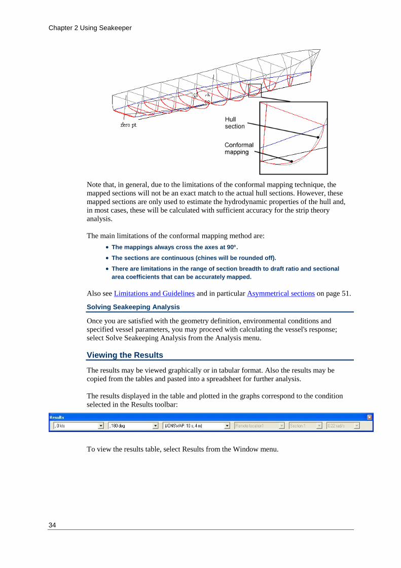
Chapter 2 Using Seakeeper
34
Note that, in general, due to the limitations of the conformal mapping technique, the
mapped sections will not be an exact match to the actual hull sections. However, these
mapped sections are only used to estimate the hydrodynamic properties of the hull and,
in most cases, these will be calculated with sufficient accuracy for the strip theory
analysis.
The main limitations of the conformal mapping method are:
The mappings always cross the axes at 90.
The sections are continuous (chines will be rounded off).
There are limitations in the range of section breadth to draft ratio and sectional
area coefficients that can be accurately mapped.
Also see Limitations and Guidelines and in particular Asymmetrical sections on page 51.
Solving Seakeeping Analysis
Once you are satisfied with the geometry definition, environmental conditions and
specified vessel parameters, you may proceed with calculating the vessel's response;
select Solve Seakeeping Analysis from the Analysis menu.
Viewing the Results
The results may be viewed graphically or in tabular format. Also the results may be
copied from the tables and pasted into a spreadsheet for further analysis.
The results displayed in the table and plotted in the graphs correspond to the condition
selected in the Results toolbar:
To view the results table, select Results from the Window menu.
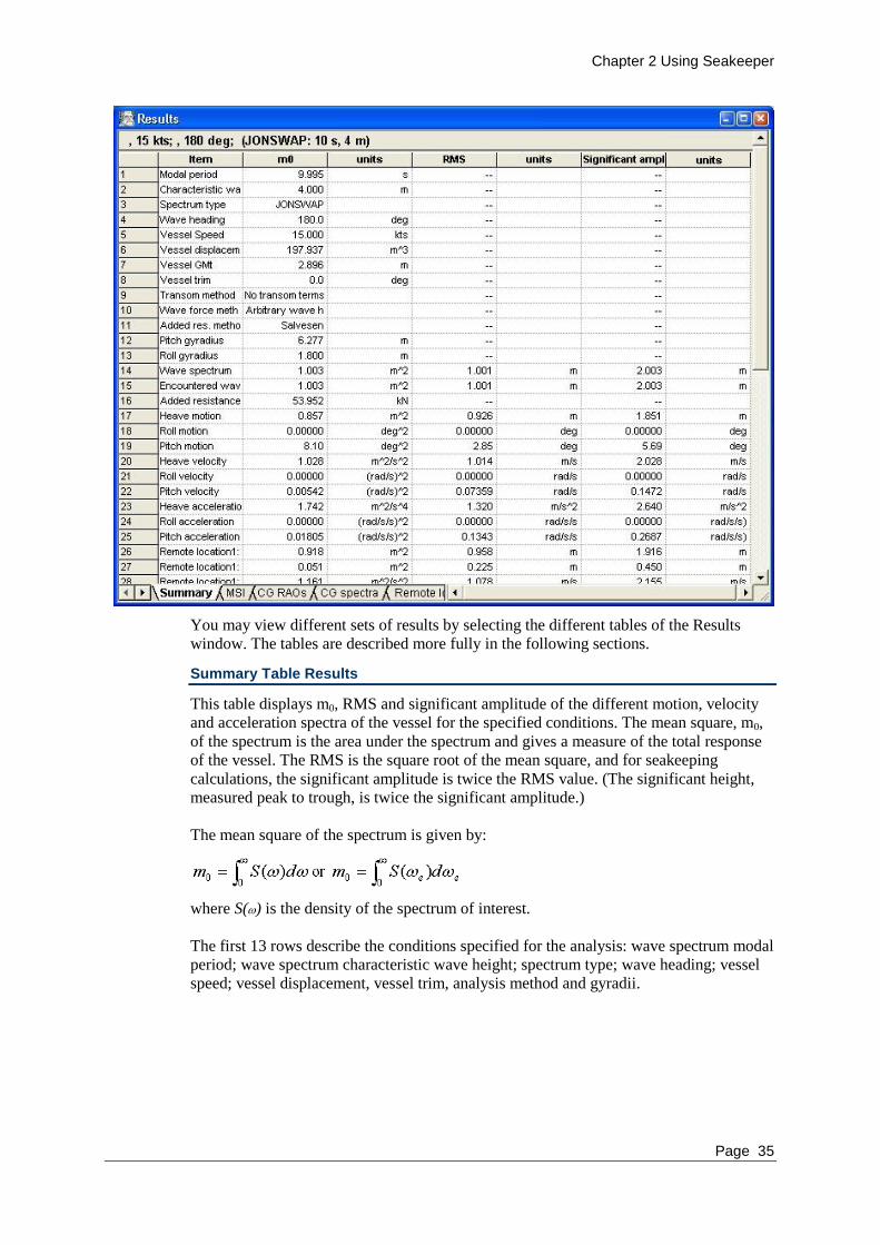
Chapter 2 Using Seakeeper
Page 35
You may view different sets of results by selecting the different tables of the Results
window. The tables are described more fully in the following sections.
Summary Table Results
This table displays m0, RMS and significant amplitude of the different motion, velocity
and acceleration spectra of the vessel for the specified conditions. The mean square, m0,
of the spectrum is the area under the spectrum and gives a measure of the total response
of the vessel. The RMS is the square root of the mean square, and for seakeeping
calculations, the significant amplitude is twice the RMS value. (The significant height,
measured peak to trough, is twice the significant amplitude.)
The mean square of the spectrum is given by:
where S() is the density of the spectrum of interest.
The first 13 rows describe the conditions specified for the analysis: wave spectrum modal
period; wave spectrum characteristic wave height; spectrum type; wave heading; vessel
speed; vessel displacement, vessel trim, analysis method and gyradii.
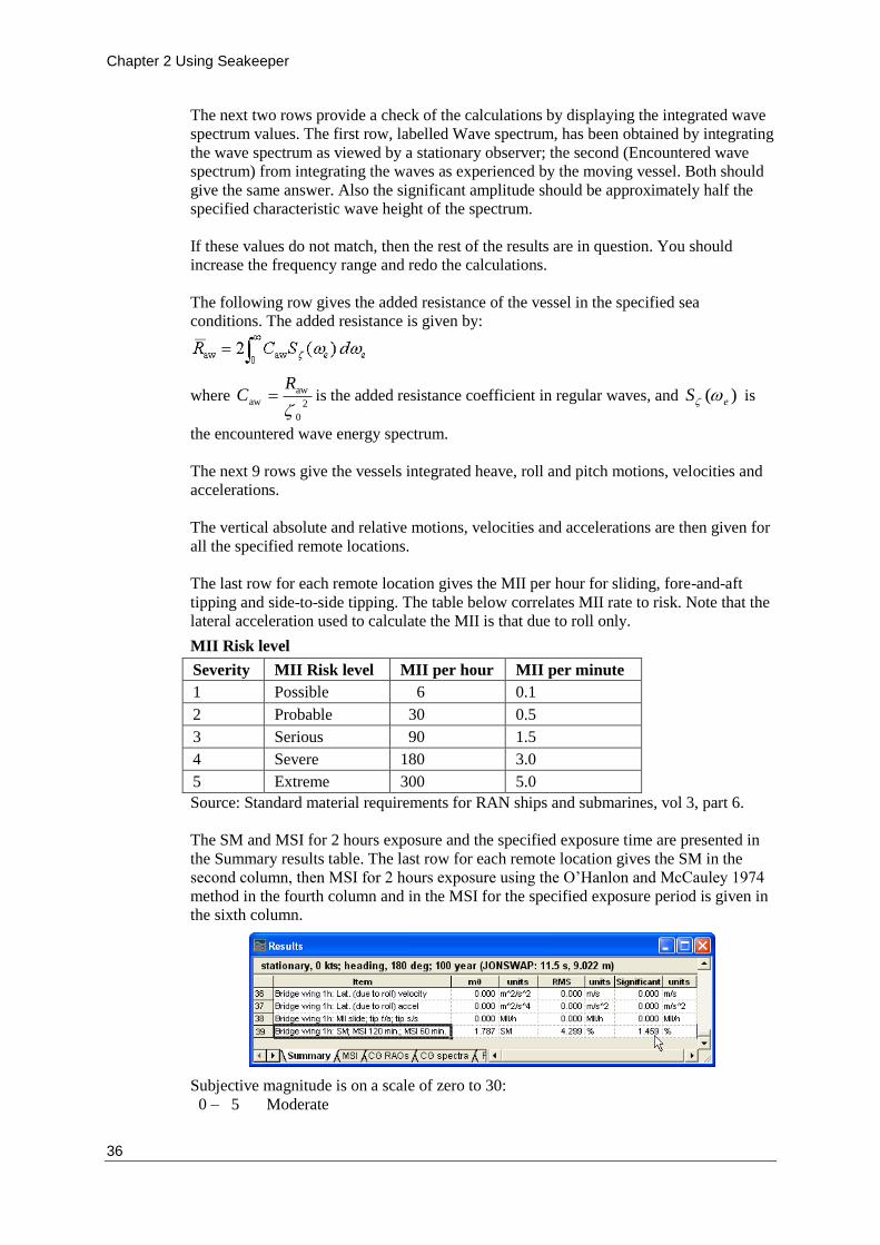
Chapter 2 Using Seakeeper
36
The next two rows provide a check of the calculations by displaying the integrated wave
spectrum values. The first row, labelled Wave spectrum, has been obtained by integrating
the wave spectrum as viewed by a stationary observer; the second (Encountered wave
spectrum) from integrating the waves as experienced by the moving vessel. Both should
give the same answer. Also the significant amplitude should be approximately half the
specified characteristic wave height of the spectrum.
If these values do not match, then the rest of the results are in question. You should
increase the frequency range and redo the calculations.
The following row gives the added resistance of the vessel in the specified sea
conditions. The added resistance is given by:
where 2
0
aw
aw
RC is the added resistance coefficient in regular waves, and )( eS is
the encountered wave energy spectrum.
The next 9 rows give the vessels integrated heave, roll and pitch motions, velocities and
accelerations.
The vertical absolute and relative motions, velocities and accelerations are then given for
all the specified remote locations.
The last row for each remote location gives the MII per hour for sliding, fore-and-aft
tipping and side-to-side tipping. The table below correlates MII rate to risk. Note that the
lateral acceleration used to calculate the MII is that due to roll only.
MII Risk level
Severity MII Risk level MII per hour MII per minute
1 Possible 6 0.1
2 Probable 30 0.5
3 Serious 90 1.5
4 Severe 180 3.0
5 Extreme 300 5.0
Source: Standard material requirements for RAN ships and submarines, vol 3, part 6.
The SM and MSI for 2 hours exposure and the specified exposure time are presented in
the Summary results table. The last row for each remote location gives the SM in the
second column, then MSI for 2 hours exposure using the O’Hanlon and McCauley 1974
method in the fourth column and in the MSI for the specified exposure period is given in
the sixth column.
Subjective magnitude is on a scale of zero to 30:
0 – 5 Moderate

Chapter 2 Using Seakeeper
Page 37
5 – 10 Serious
10 – 15 Severe: necessary to “hang on”
15 – 20 Hazardous
20 – 30 Intolerable
See: Calculation of Subjective Magnitude and Motion Sickness Incidence on page 81 for
details of the calculations performed.
The majority of the results calculated in the Summary table may be plotted in the Polar
Plot window provide that the response for at least two speeds and a range of headings has
been calculated.
MSI – ISO 2631/3 1985 and BS 6841:1987 Results
Although not strictly MSI accelerations integrated over 1/3 octave bins are plotted
against acceleration limits defined by these two standards. The likely discomfort can be
gauged by how close these acceleration curves approach the defined acceleration limits.
The second table gives the acceleration curves at the specified remote locations. The data
for the standard ISO and BSI curves are also given. The MSI acceleration is calculated
from the equation below:
where the frequency interval e1 to e2 is the 1/3 octave range centred about e centre and
Svert accel is the absolute vertical acceleration at the point of interest on the vessel.
Existing comparison of accelerations compared with ISO and BS standards
CG RAO Results
The next table gives the computed vessel RAOs for the principal degrees of freedom, at
the vessel's centre of gravity. These have been non-dimensionalised with wave height for
heave and with wave slope for roll and pitch motions. The phase lag of the motions is
also given.
Finally the added resistance coefficient in regular waves, 2
0
aw
aw
RC , is given. This
value is dimensional, and has units of Force / Length2. There are several accepted ways
of non-dimensionalising added resistance. Gerritsma and Beukelman use the following:
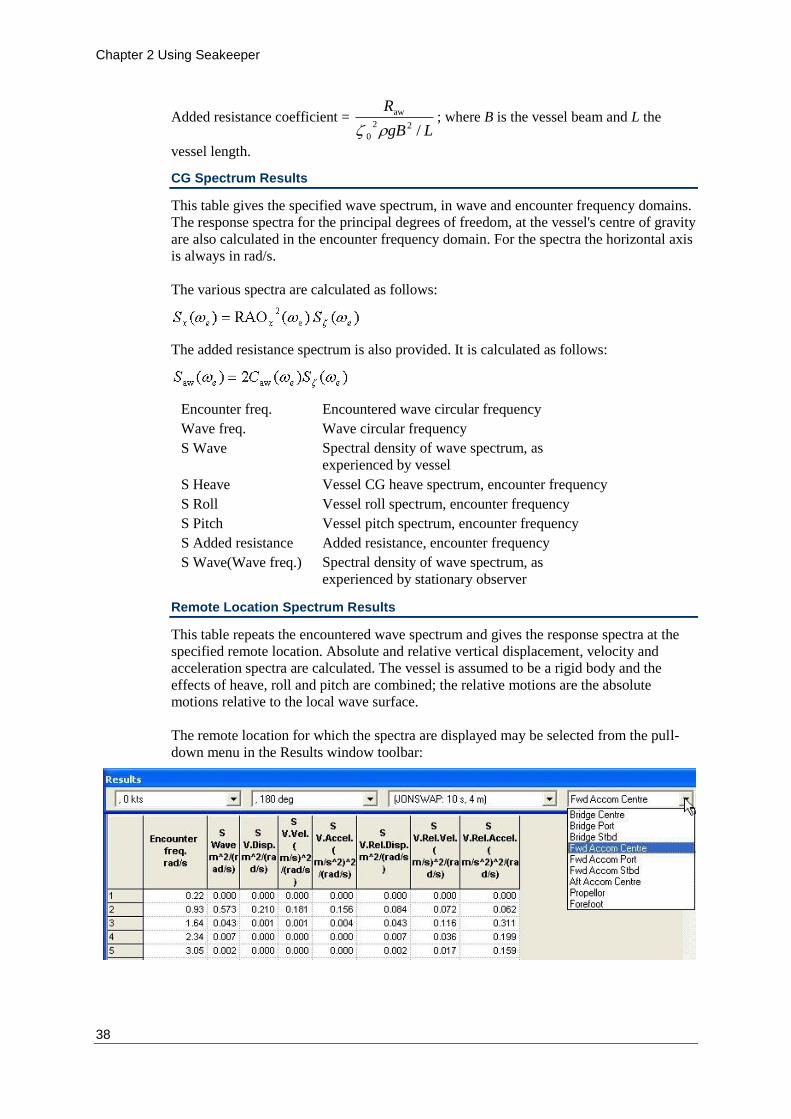
Chapter 2 Using Seakeeper
38
Added resistance coefficient = LgB
R
/22
0
aw
; where B is the vessel beam and L the
vessel length.
CG Spectrum Results
This table gives the specified wave spectrum, in wave and encounter frequency domains.
The response spectra for the principal degrees of freedom, at the vessel's centre of gravity
are also calculated in the encounter frequency domain. For the spectra the horizontal axis
is always in rad/s.
The various spectra are calculated as follows:
The added resistance spectrum is also provided. It is calculated as follows:
Encounter freq. Encountered wave circular frequency
Wave freq. Wave circular frequency
S Wave Spectral density of wave spectrum, as
experienced by vessel
S Heave Vessel CG heave spectrum, encounter frequency
S Roll Vessel roll spectrum, encounter frequency
S Pitch Vessel pitch spectrum, encounter frequency
S Added resistance Added resistance, encounter frequency
S Wave(Wave freq.) Spectral density of wave spectrum, as
experienced by stationary observer
Remote Location Spectrum Results
This table repeats the encountered wave spectrum and gives the response spectra at the
specified remote location. Absolute and relative vertical displacement, velocity and
acceleration spectra are calculated. The vessel is assumed to be a rigid body and the
effects of heave, roll and pitch are combined; the relative motions are the absolute
motions relative to the local wave surface.
The remote location for which the spectra are displayed may be selected from the pull-
down menu in the Results window toolbar:

Chapter 2 Using Seakeeper
Page 39
Encounter freq. Encountered wave circular frequency
S Wave Spectral density of wave spectrum, as experienced by vessel
S V.Disp. Absolute vertical displacement spectrum, encounter
frequency
S V.Vel. Absolute vertical velocity spectrum, encounter frequency
S V.Accel. Absolute vertical acceleration spectrum, encounter
frequency
S V.Rel.Disp. Relative vertical displacement spectrum, encounter
frequency
S V.Rel.Vel. Relative vertical velocity spectrum, encounter frequency
S V.Rel.Accel. Relative vertical acceleration spectrum, encounter frequency
Global Hydrodynamic coefficients
These are the integrated coefficients, cross-coupling terms and excitation forces in the
equations of motion of the vessel. These are the total values for the complete vessel.
Encounter freq. Encountered wave circular frequency
Mass + added mass33 Total vessel mass and added mass at specified
encounter freq.
Added mass35 Cross-coupling heave added mass due to pitch
Added inertia53 Cross-coupling pitch added inertia due to heave
Inertia + added inertia55 Total vessel inertia and added inertia in pitch
Damping33 Heave inviscid damping
Damping35 Heave/Pitch cross-coupling damping
Damping53 Pitch /Heave cross-coupling damping
Damping55 Pitch inviscid damping
Stiffness33 Heave stiffness (restoring force term)
Stiffness35 Heave/Pitch cross-coupling stiffness
Stiffness53 Pitch / Heave cross-coupling stiffness
Stiffness55 Heave stiffness (restoring force term)
Wave excitation3 Total wave excitation amplitude in heave
Wave excitation Phase3 Heave wave excitation phase
Wave excitation5 Total wave excitation amplitude in pitch
Wave excitation Phase5 Heave wave excitation phase
Sectional Hydrodynamic Coefficient Results (Strip theory)
The added mass, damping, stiffness and wave excitation for each of the sections of the
hull at each of the frequencies of interest. For each frequency, these values are integrated
along the vessel's length to give the global coefficients in the equations of motion.
The remote location for which the spectra are displayed may be selected from the pull-
down menu in the Results window toolbar:

Chapter 2 Using Seakeeper
40
Choosing a section from the pull down menu, will display the variation of terms with
frequency for the selected section; similarly, selecting a frequency will display the
variation of terms along the length of the vessel for the selected frequency.
Section Section number from bow
Encounter freq. Encountered wave circular frequency
Mapping Terms in Lewis mapping
Added mass3 Section added mass for vertical motion
Damping3 Section inviscid damping for vertical motion
Stiffness3 Section restoring force term for vertical
motion
Froude-Krilov Wave excitation3 Amplitude of Froude-Krilov component of
wave excitation for vertical motion
Froude-Krilov Wave excitation
Phase3
Phase of Froude-Krilov component of wave
excitation for vertical motion
Diffraction Wave excitation3 Amplitude of diffraction component of wave
excitation for vertical motion
Diffraction Wave excitation
Phase3
Phase of diffraction component of wave
excitation for vertical motion
Panel Pressures
The panel pressures table displays the panel pressure values for the selected frequency.
By default values for all the panels are displayed, alternatively the user can specify just to
see just the results for the panel of interest (select from the drop down list on the results
toolbar).
The magnitude and phase of the pressure are shown. In addition the magnitude of the
Incident, Diffraction and Radiation components of the pressure are shown. The non-
dimensional values are displayed. The pressure values are non-dimensionalised
according to the water density (ρ), gravity(g) and wave amplitude (A):
Pressure’=Pressure/ρgA
Drift Forces
Drift forces and moments are displayed in the Drift Forces table. Each row representing
the value for a single frequency and heading. The values displayed are non-dimensional.
Drift forces (surge, sway and heave) are non-dimensionalised according to water density
(ρ), gravity(g), characteristic length (L) and wave amplitude (A):

Chapter 2 Using Seakeeper
Page 41
Drift force’=Drift force/ρgLA2
Drift moments (roll, pitch and yaw) are non-dimensionalised according to water density
(ρ), gravity(g), characteristic length (L) and wave amplitude (A):
Drift moment’=Drift moment/ρgL2A
2
Characteristic length defaults to the vessel’s maximum dimension. The characteristic
length can be altered by the user in the Analysis | Mesh Hull… dialog.
Wave Excitation Forces
Wave excitation forces are displayed in the wave excitation forces table. Each row
represents the exciting force in each of the 6 degrees of freedom for a frequency and
heading. The non-dimensional force magnitude and phase are presented for surge, sway,
heave, roll, pitch and yaw respectively.
Wave excitation forces (surge, sway and heave) are non-dimensionalised according to
water density (rho), gravity(g), displaced volume (▽), characteristic length (L) and wave
amplitude (A):
Wave Force’=Wave Force/( ρ g▽A/L)
Wave excitation moments (roll, pitch and yaw) are non-dimensionalised according to
water density (rho), gravity(g), displaced volume (▽) and wave amplitude (A):
Wave Force’=Wave Force/( ρ g▽A)
Characteristic length defaults to the vessel’s maximum dimension. The characteristic
length can be altered by the user in the Analysis | Mesh Hull… dialog.
Added Mass and Damping
Added mass and damping results are displayed in the Added Mass and Damping table of
the results window. The 6x6 Added Mass (Aij) and Damping (Bij) coefficient matricies
are presented for each frequency.
The coefficients are non dimensionalised using water density (ρ), gravity (g), volumetric
displacement (▽), wave amplitude (A), wave frequency(ω) and characteristic length (L).
For the added mass coefficients (Aij) the values are non-dimensionalised as follows:
i=1-3 and j=1-3: Aij’=Aij/( ρ▽)
i=1-3 and j=4-6: Aij’=Aij/( ρ▽L)
i=4-6 and j=1-3: Aij’=Aij/( ρ▽L)
i=4-6 and j=4-6: Aij’=Aij/( ρ▽L2)
For the added mass coefficients (Bij) the values are non-dimensionalised as follows:
i=1-3 and j=1-3: Bij’=Bij/( ρ▽ω)
i=1-3 and j=4-6: Bij’=Bij/( ρ▽L ω)
i=4-6 and j=1-3: Bij’=Bij/( ρ▽L ω)
i=4-6 and j=4-6: Bij’=Bij/( ρ▽L2 ω)

Chapter 2 Using Seakeeper
42
Graphing the Results
All the above datasheets, except for the integrated values, may be graphed and displayed
in the graph window:
MSI
RAO
CG Spectra
Remote Spectra
Global Hydrodynamics
Section Hydrodynamics
To select the desired graph, make the graph window the uppermost window by either
clicking in the window or selecting Graph from the bottom of the Window menu.
The desired datasheet may now be selected from the Window menu: select Graph and
drag right to display the available graphs.
Once a graph has been chosen, the various data sets in the graph may be turned on or off.
To do this, select Graph Options from the Display menu. The following dialog will be
displayed. If the current graph is of the response spectra, it will not be possible to change
the frequency scale.
Turn on the desired data sets; and
Select the desired horizontal axis format.

Chapter 2 Using Seakeeper
Page 43
The section data (Sectional forces and Sectional hydrodynamic coefficients) may be
plotted and displayed against frequency (for a single section) or against section position
(for a single frequency). In addition it is possible to display all the data in the Results
datasheet, but in this case the data will not be plotted. To change the format, choose
Section Data from the Display menu:
To plot data for a single section, select the Section radio button and type the number of
the section for which you want the data in the Current section edit box. To plot the
variation along the length of the hull, for a single frequency, select the Frequency radio
button and type the frequency of interest in the Current frequency box. To display all the
data, select the Display all data – note that, in this case, the data will be displayed in the
table only and not in the graph.
Sections start with number 1 at the bow and increment towards the stern. In Plan or
Profile views, the station numbers are displayed once the hull has been measured.
Some of the graphing options may be accessed more quickly using the Graph toolbar:
Use the combo box to select which data you would like to graph and the Graph Options
button, to edit which lines are shown and the horizontal scale.
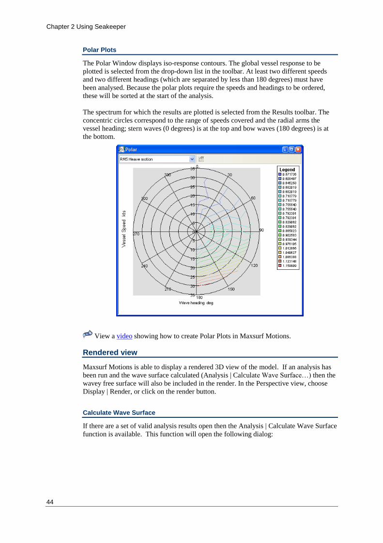
Chapter 2 Using Seakeeper
44
Polar Plots
The Polar Window displays iso-response contours. The global vessel response to be
plotted is selected from the drop-down list in the toolbar. At least two different speeds
and two different headings (which are separated by less than 180 degrees) must have
been analysed. Because the polar plots require the speeds and headings to be ordered,
these will be sorted at the start of the analysis.
The spectrum for which the results are plotted is selected from the Results toolbar. The
concentric circles correspond to the range of speeds covered and the radial arms the
vessel heading; stern waves (0 degrees) is at the top and bow waves (180 degrees) is at
the bottom.
View a video showing how to create Polar Plots in Maxsurf Motions.
Rendered view
Maxsurf Motions is able to display a rendered 3D view of the model. If an analysis has
been run and the wave surface calculated (Analysis | Calculate Wave Surface…) then the
wavey free surface will also be included in the render. In the Perspective view, choose
Display | Render, or click on the render button.
Calculate Wave Surface
If there are a set of valid analysis results open then the Analysis | Calculate Wave Surface
function is available. This function will open the following dialog:

Chapter 2 Using Seakeeper
Page 45
There are three options for the free surface: static (flat) and, once the analysis has been
performed, regular and irregular wavy surfaces may be used. At the bottom of the dialog
are some options for displaying of panel pressures during an animation in a regular or
irregular seaway. If the “Smooth shading” option is shown the pressures will be
“smoothed” over the panels, if smooth shading is not checked then the actual calculated
pressure for the entire panel is rendered. The panel pressure options are not applicable to
the strip theory method.
Static (flat) free surface
With this method selected, no free surface elevation is calculated.

Chapter 2 Using Seakeeper
46
Static (flat) free surface
Roll decay simulation
With this method selected, no free surface elevation is calculated, however when you
select Animate from the Display menu, a simulation of a free roll decay test will be
displayed. This simulates the roll motion of a vessel heeled over to a specified initial roll
angle and then released. The initial heel angle is held for 5 seconds, then the vessel is
released.
To conduct a roll decay simulation, follow these steps:
Make sure you have specified all Seakeeping input data correctly by working your
way down the analysis menu
Solve Seakeeping Analysis from the analysis menu
Calculate Wave Surface from the analysis menu
Select Roll decay simulation in the dialog that appears
Specify the initial heel angle
Select Animate from the display menu (make sure you are in the Perspective View)
Click OK
Note:
Saving the roll decay as a text file and then importing into Excel may help
you further analyse the Roll decay simulation data.
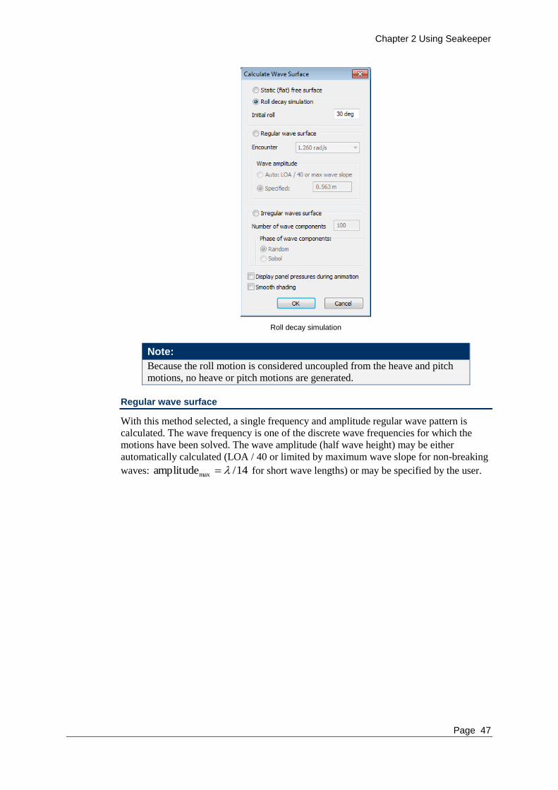
Chapter 2 Using Seakeeper
Page 47
Roll decay simulation
Note:
Because the roll motion is considered uncoupled from the heave and pitch
motions, no heave or pitch motions are generated.
Regular wave surface
With this method selected, a single frequency and amplitude regular wave pattern is
calculated. The wave frequency is one of the discrete wave frequencies for which the
motions have been solved. The wave amplitude (half wave height) may be either
automatically calculated (LOA / 40 or limited by maximum wave slope for non-breaking
waves: 14/amplitudemax for short wave lengths) or may be specified by the user.

Chapter 2 Using Seakeeper
48
Regular wave surface
Irregular wave surface
The final option allows an irregular wave pattern to be calculated based on the selected
wave spectrum. The irregular wave pattern is calculated by superimposing linear regular
sine-wave components. The number of wave components to be used can be changed by
the user. The wave components are chosen so that the wave energy in each frequency is
the same; each component is then given a random phase. If you have a slower computer,
it may be necessary to reduce the number of wave components used; increasing the
number of wave components will increase the detail with which the wavy surface and
vessel motions are calculated.
Either Random or Sobol quasi-random distribution can be used for the wave component
phases. The Sobol sequence is quasi-random but will always be the same. This gives a
repeatable random sea state which allows the time simulation to be carried out for
different models but using the same wave-trace. The Random option uses the computer’s
random function to generate a wave trace that will be different every time.

Chapter 2 Using Seakeeper
Page 49
Irregular wave surface
Wavy surface display
Once the wavy surface has been calculated it may be displayed. A grid representing the
wavy surface may be turned on by selecting the Wave Surface option in the Display |
Visibility dialog:
Note
The wavy surface grid uses the Net colour as defined in the View | Colour
dialog.

Chapter 2 Using Seakeeper
50
The wavy surface may also be displayed by turning on the rendering (Display | Render).
In either display mode, the wavy surface grid may be turned on or off in the Display |
Visibility dialog (as described above) or by using the Wave Grid button in the Contours
toolbar: .
Time Simulation and Animation
After calculating the wave surface (see Rendered view on page 41), Maxsurf Motions is
able to animate the vessel for the specified initial roll decay angle or in the selected wave
pattern. Choose Display | Animate to start the animation and use the Escape (Esc) key to
terminate the animation.
Animation of the vessel motions may be displayed when either a regular or irregular
wave surface has been calculated. If you try to animate the model with a flat free-surface,
you will get the following error message:

Chapter 2 Using Seakeeper
Page 51
If a wavy surface has been calculated, the animate dialog will be displayed; this gives
you the option of saving the time series data to a text file. The text file contains the
statistics and time series for wave elevation and heave, roll and pitch motions.
By default, the animation is displayed in real time; the frame rate is adapted so that the
animation is in real time. If you have a slow computer or graphics card (hardware
accelerated OpenGL graphics cards will generally increase the frame rate) then the frame
rate may be too low to provide a reasonable animation. If this is the case you can reduce
the attempted play back speed; use the keypad “-” key to slow down the animation which
will increase the frame rate, or use the keypad “+” key to speedup the animation which
will reduce the frame rate.
The instantaneous time, heave, roll and pitch are displayed in the status bar when the
animation takes place:
If the panel pressures are being displayed a legend will appear in the top right of the
rendered view, displaying which colours correspond with which panel pressure:
Vessel heading, speed and wave spectrum
The vessel heading, speed and wave spectrum used in the animation is selected from the
pull down boxes in the Results toolbar (only results that have actually been evaluated
may be chosen):
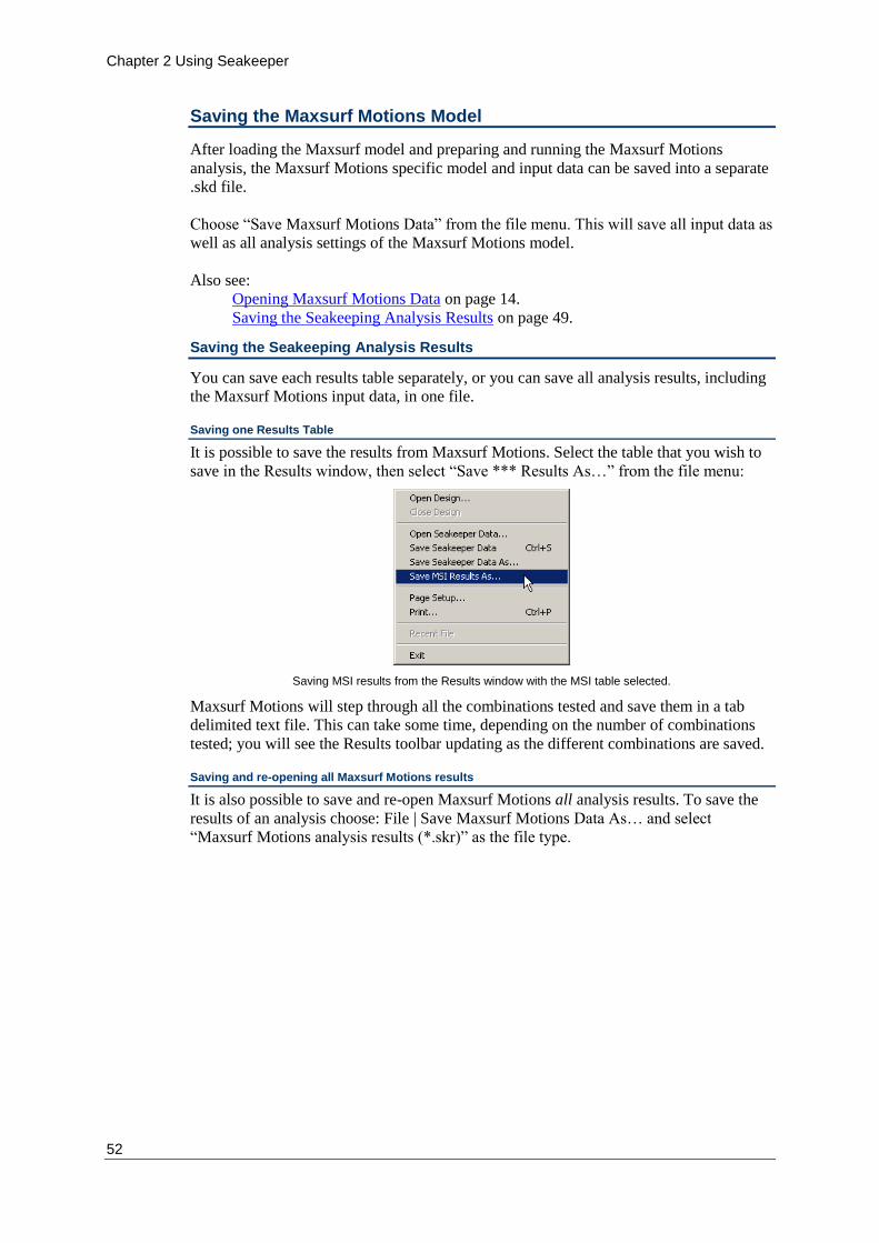
Chapter 2 Using Seakeeper
52
Saving the Maxsurf Motions Model
After loading the Maxsurf model and preparing and running the Maxsurf Motions
analysis, the Maxsurf Motions specific model and input data can be saved into a separate
.skd file.
Choose “Save Maxsurf Motions Data” from the file menu. This will save all input data as
well as all analysis settings of the Maxsurf Motions model.
Also see:
Opening Maxsurf Motions Data on page 14.
Saving the Seakeeping Analysis Results on page 49.
Saving the Seakeeping Analysis Results
You can save each results table separately, or you can save all analysis results, including
the Maxsurf Motions input data, in one file.
Saving one Results Table
It is possible to save the results from Maxsurf Motions. Select the table that you wish to
save in the Results window, then select “Save *** Results As…” from the file menu:
Saving MSI results from the Results window with the MSI table selected.
Maxsurf Motions will step through all the combinations tested and save them in a tab
delimited text file. This can take some time, depending on the number of combinations
tested; you will see the Results toolbar updating as the different combinations are saved.
Saving and re-opening all Maxsurf Motions results
It is also possible to save and re-open Maxsurf Motions all analysis results. To save the
results of an analysis choose: File | Save Maxsurf Motions Data As… and select
“Maxsurf Motions analysis results (*.skr)” as the file type.
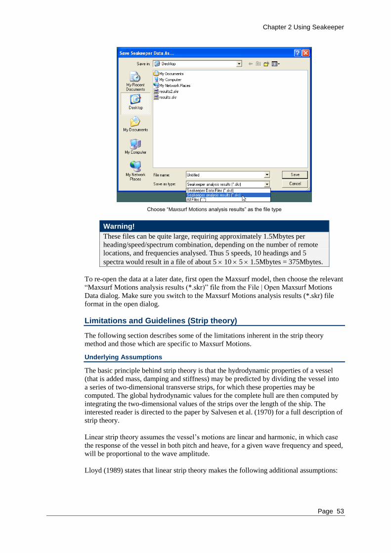
Chapter 2 Using Seakeeper
Page 53
Choose “Maxsurf Motions analysis results” as the file type
Warning!
These files can be quite large, requiring approximately 1.5Mbytes per
heading/speed/spectrum combination, depending on the number of remote
locations, and frequencies analysed. Thus 5 speeds, 10 headings and 5
spectra would result in a file of about 5 10 5 1.5Mbytes = 375Mbytes.
To re-open the data at a later date, first open the Maxsurf model, then choose the relevant
“Maxsurf Motions analysis results (*.skr)” file from the File | Open Maxsurf Motions
Data dialog. Make sure you switch to the Maxsurf Motions analysis results (*.skr) file
format in the open dialog.
Limitations and Guidelines (Strip theory)
The following section describes some of the limitations inherent in the strip theory
method and those which are specific to Maxsurf Motions.
Underlying Assumptions
The basic principle behind strip theory is that the hydrodynamic properties of a vessel
(that is added mass, damping and stiffness) may be predicted by dividing the vessel into
a series of two-dimensional transverse strips, for which these properties may be
computed. The global hydrodynamic values for the complete hull are then computed by
integrating the two-dimensional values of the strips over the length of the ship. The
interested reader is directed to the paper by Salvesen et al. (1970) for a full description of
strip theory.
Linear strip theory assumes the vessel’s motions are linear and harmonic, in which case
the response of the vessel in both pitch and heave, for a given wave frequency and speed,
will be proportional to the wave amplitude.
Lloyd (1989) states that linear strip theory makes the following additional assumptions:

Chapter 2 Using Seakeeper
54
The fluid is inviscid – viscous damping is ignored, (In fact the damping factor
which the user enters for roll should include viscous roll damping, which is the
primary source of damping for roll.)
The ship is slender (i.e. the length is much greater than the beam or the draft, and
the beam is much less than the wave length).
The hull is rigid so that no flexure of the structure occurs.
The speed is moderate so there is no appreciable planing lift.
The motions are small (or at least linear with wave amplitude).
The ship hull sections are wall-sided.
The water depth is much greater than the wave length so that deep water wave
approximations may be applied.
The presence of the hull has no effect on the waves (Froude-Krilov hypothesis.)
In addition, the principle of superposition is used to compute the response of the vessel to
irregular waves. Simply, this means that the contributions to the motions of the
individual regular waves making up the irregular sea spectrum may be summed to obtain
the total response of the vessel to the irregular seas.
Boyd (1995) outlines possible causes of non-linear behaviour, or effects that may cause
strip theory to become inaccurate, such as:
Emergence or submergence of the bow or stern.
Flare (non-wall sidedness) of the hull at the waterplane.
Submergence of the bow or stern overhangs in a vessel.
Three dimensional flow effects and flow interaction in a longitudinal direction along
the hull including dynamic lift at speed.
Increasing importance of wave diffraction, wave radiation and the Kelvin wave
pattern at speed.
At present, Maxsurf Motions is based upon linear theory, however, in the future, it is
intended to include options to account for some of the geometric non-linearities
mentioned above.
Asymmetrical sections
Whilst not being able to actually represent asymmetrical hulls in the hydrodynamic
model, Maxsurf Motions can approximate asymmetric hulls by correctly measuring the
sections’ cross-sectional area and waterline beam. This is shown for the asymmetric
catamaran demihull below. Here the asymmetrical hull sections are shown in black and
the mapped symmetrical sections are shown in red.

Chapter 2 Using Seakeeper
Page 55
See Calculation of Mapped Sections on page 29 for information on mapping sections.
Vessel Speed
Generally strip theory is applied to vessels operating at low to moderate Froude number.
However, experience has shown that reasonable predictions may be made for Froude
numbers approaching 0.8, provided that the vessel is quite slender. It should also be
remembered that dynamic vertical forces due to forward speed are not included, hence
Maxsurf Motions is likely to over-estimate the motions of planing vessels operating in
the planing regime.
The panel method is based on a zero speed Green’s function and as such is only valid for
the zero forward speed case. A non zero forward speed may be set however the user will
get a warning when the analysis is started. Running a panel method analysis at speeds
other than zero will conduct the seakeeping analysis at the modified encounter frequency.
This approximation for low speeds (Fn<~0.1) may be a valid approach for some
applications.
Wave Heading
At present Maxsurf Motions uses strip theory to predict vertical plane motions. The roll
motion is simply estimated assuming a damped spring/mass system. The computations
have been found to be most reliable from head seas (180deg.) to bow-quartering seas
(135, 215deg.). For these calculations, the head seas approximation for the wave
excitation force and moment is normally sufficiently accurate. As the wave heading
moves more to beam seas, the arbitrary wave heading method should be used to calculate
the wave excitation. However, due to the lack of available data, this formulation has not
been rigorously tested.
Strip theory calculations for following seas are less accurate, since the motions become
much less linear. Calculations made with Maxsurf Motions (or any frequency domain,
strip theory program) for these conditions, should be treated with caution and, if possible,
validated by other means.
Because of the non-unique mapping of encounter frequency to wave frequency in
following waves (i.e. in some cases it is possible to get the same encounter frequency
from three different wave frequencies) MSI calculations in following seas are unreliable.

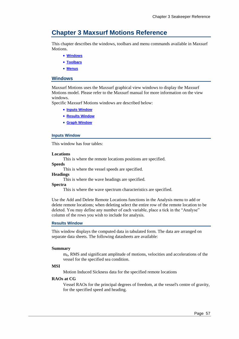
Chapter 3 Seakeeper Reference
Page 57
Chapter 3 Maxsurf Motions Reference
This chapter describes the windows, toolbars and menu commands available in Maxsurf
Motions.
Windows
Toolbars
Menus
Windows
Maxsurf Motions uses the Maxsurf graphical view windows to display the Maxsurf
Motions model. Please refer to the Maxsurf manual for more information on the view
windows.
Specific Maxsurf Motions windows are described below:
Inputs Window
Results Window
Graph Window
Inputs Window
This window has four tables:
Locations This is where the remote locations positions are specified.
Speeds
This is where the vessel speeds are specified.
Headings This is where the wave headings are specified.
Spectra This is where the wave spectrum characteristics are specified.
Use the Add and Delete Remote Locations functions in the Analysis menu to add or
delete remote locations; when deleting select the entire row of the remote location to be
deleted. You may define any number of each variable, place a tick in the “Analyse”
column of the rows you wish to include for analysis.
Results Window
This window displays the computed data in tabulated form. The data are arranged on
separate data sheets. The following datasheets are available:
Summary
m0, RMS and significant amplitude of motions, velocities and accelerations of the
vessel for the specified sea condition.
MSI
Motion Induced Sickness data for the specified remote locations
RAOs at CG
Vessel RAOs for the principal degrees of freedom, at the vessel's centre of gravity,
for the specified speed and heading.

Chapter 3 Seakeeper Reference
58
Spectra at CG
Wave and response spectra for the principal degrees of freedom, at the vessel's
centre of gravity.
Spectra at remote location
Wave and response spectra for the principal degrees of freedom, at the vessel's
centre of gravity.
Global hydrodynamic coefficients
Global coefficients, cross-coupling terms and excitation forces in the equations of
motion.
Sectional hydrodynamic coefficients
Added mass, damping, stiffness and wave excitation for each of the sections at
each of the frequencies of interest.
Panel Pressures (not applicable to strip theory)
Panel pressure magnitudes and phases for each panel at each of the headings and
frequencies of interest. Including incident, diffraction and radiation components.
Drift Forces (not applicable to strip theory)
Drift forces and moments in each degree of freedom for frequencies and headings
of interest.
Wave Excitation Forces (not applicable to strip theory)
Wave excitation forces and moments (and phases) in each degree of freedom for
frequencies and headings of interest.
Added Mass and Damping (not applicable to strip theory)
Added Mass and wave damping matrix for frequencies and headings of interest.
Depending on which table is selected, you may use the pull-down menus in the Results
toolbar to select which data are displayed:
Graph Window
The above data may also be displayed in graphical form. To display the data in graphical
format choose Graph from the Window menu or click on the graph button.
The different data sets within the datasheet may be turned on or off by selecting Graph
Options from the Display menu. The x-axis scale may also be changed in this dialog.
The Graph window Toolbar allows you to quickly select which graph is displayed and
adjust which lines are drawn on the graph:
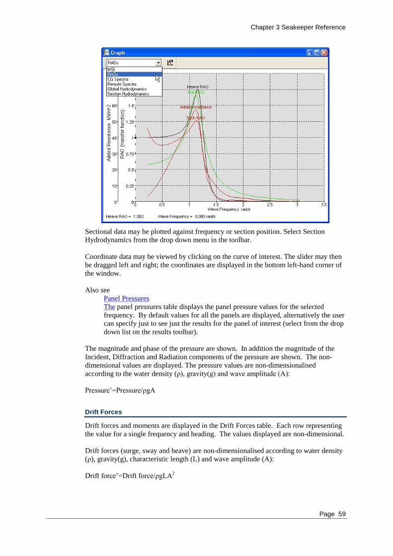
Chapter 3 Seakeeper Reference
Page 59
Sectional data may be plotted against frequency or section position. Select Section
Hydrodynamics from the drop down menu in the toolbar.
Coordinate data may be viewed by clicking on the curve of interest. The slider may then
be dragged left and right; the coordinates are displayed in the bottom left-hand corner of
the window.
Also see
Panel Pressures
The panel pressures table displays the panel pressure values for the selected
frequency. By default values for all the panels are displayed, alternatively the user
can specify just to see just the results for the panel of interest (select from the drop
down list on the results toolbar).
The magnitude and phase of the pressure are shown. In addition the magnitude of the
Incident, Diffraction and Radiation components of the pressure are shown. The non-
dimensional values are displayed. The pressure values are non-dimensionalised
according to the water density (ρ), gravity(g) and wave amplitude (A):
Pressure’=Pressure/ρgA
Drift Forces
Drift forces and moments are displayed in the Drift Forces table. Each row representing
the value for a single frequency and heading. The values displayed are non-dimensional.
Drift forces (surge, sway and heave) are non-dimensionalised according to water density
(ρ), gravity(g), characteristic length (L) and wave amplitude (A):
Drift force’=Drift force/ρgLA2

Chapter 3 Seakeeper Reference
60
Drift moments (roll, pitch and yaw) are non-dimensionalised according to water density
(ρ), gravity(g), characteristic length (L) and wave amplitude (A):
Drift moment’=Drift moment/ρgL2A
2
Characteristic length defaults to the vessel’s maximum dimension. The characteristic
length can be altered by the user in the Analysis | Mesh Hull… dialog.
Wave Excitation Forces
Wave excitation forces are displayed in the wave excitation forces table. Each row
represents the exciting force in each of the 6 degrees of freedom for a frequency and
heading. The non-dimensional force magnitude and phase are presented for surge, sway,
heave, roll, pitch and yaw respectively.
Wave excitation forces (surge, sway and heave) are non-dimensionalised according to
water density (rho), gravity(g), displaced volume (▽), characteristic length (L) and wave
amplitude (A):
Wave Force’=Wave Force/( ρ g▽A/L)
Wave excitation moments (roll, pitch and yaw) are non-dimensionalised according to
water density (rho), gravity(g), displaced volume (▽) and wave amplitude (A):
Wave Force’=Wave Force/( ρ g▽A)
Characteristic length defaults to the vessel’s maximum dimension. The characteristic
length can be altered by the user in the Analysis | Mesh Hull… dialog.
Added Mass and Damping
Added mass and damping results are displayed in the Added Mass and Damping table of
the results window. The 6x6 Added Mass (Aij) and Damping (Bij) coefficient matricies
are presented for each frequency.
The coefficients are non dimensionalised using water density (ρ), gravity (g), volumetric
displacement (▽), wave amplitude (A), wave frequency(ω) and characteristic length (L).
For the added mass coefficients (Aij) the values are non-dimensionalised as follows:
i=1-3 and j=1-3: Aij’=Aij/( ρ▽)
i=1-3 and j=4-6: Aij’=Aij/( ρ▽L)
i=4-6 and j=1-3: Aij’=Aij/( ρ▽L)
i=4-6 and j=4-6: Aij’=Aij/( ρ▽L2)
For the added mass coefficients (Bij) the values are non-dimensionalised as follows:
i=1-3 and j=1-3: Bij’=Bij/( ρ▽ω)
i=1-3 and j=4-6: Bij’=Bij/( ρ▽L ω)
i=4-6 and j=1-3: Bij’=Bij/( ρ▽L ω)
i=4-6 and j=4-6: Bij’=Bij/( ρ▽L2 ω)
Graphing the Results on page 36
Results Toolbar on page 56
Graph window Toolbar on page 56

Chapter 3 Seakeeper Reference
Page 61
Polar Window
See Polar Plots on page 40 for information on the Polar Plot graph.
Toolbars
Some of the features of Maxsurf Motions can be accessed using the icons on the toolbars.
You can hold your mouse over an icon to reveal a pop-up tip of what the icon does.
File Toolbar
The File toolbar contains icons that execute the following commands:
New – Open Maxsurf file– Save Maxsurf Motions Input data| Cut - Copy - Paste | Print
View Toolbar
The View toolbar contains icons that execute the following commands:
Zoom – Shrink – Pan – Home View – Rotate – Assembly window (disabled).
The Rotate command is only available in the Perspective window. The Assembly
window is not available in Maxsurf Motions.
Analysis Toolbar
The Analysis toolbar contains an icon that starts the analysis: Solve Seakeeping Analysis
Contour Toolbar
The Contours toolbar contains icons that facilitate the display of surface contours:
Sections – Waterlines – Mapped Sections | Wave Grid
Window Toolbar
The Window toolbar contains icons that make the corresponding window come to the
front:
Perspective – Plan – Profile – Body Plan – Input Data – Results Data – Results Graph –
Polar Plot – Sectional Area Curve
Results Toolbar
The Results Window toolbar contains icons that allow you to quickly choose which
analysis run is displayed. Menus that are irrelevant to the currently active table are
greyed out and unavailable for selection:
Speed – Heading – Spectrum – Remote Location – Section – Encounter Frequency –
Panel Number

Chapter 3 Seakeeper Reference
62
Graph window Toolbar
The Window toolbar contains icons that facilitate swapping between the different graph
types. Use the Results toolbar to select the data for the desired analysis run and dataset,
for example: using the results toolbar you can display the remote spectrum graph for the
Bridge Centre for a JONSWAP 10s 4m headseas condition at 15 kts. See the Results
Toolbar paragraph above for more information.
Also see
Panel Pressures
The panel pressures table displays the panel pressure values for the selected
frequency. By default values for all the panels are displayed, alternatively the user
can specify just to see just the results for the panel of interest (select from the drop
down list on the results toolbar).
The magnitude and phase of the pressure are shown. In addition the magnitude of the
Incident, Diffraction and Radiation components of the pressure are shown. The non-
dimensional values are displayed. The pressure values are non-dimensionalised
according to the water density (ρ), gravity(g) and wave amplitude (A):
Pressure’=Pressure/ρgA
Drift Forces
Drift forces and moments are displayed in the Drift Forces table. Each row representing
the value for a single frequency and heading. The values displayed are non-dimensional.
Drift forces (surge, sway and heave) are non-dimensionalised according to water density
(ρ), gravity(g), characteristic length (L) and wave amplitude (A):
Drift force’=Drift force/ρgLA2
Drift moments (roll, pitch and yaw) are non-dimensionalised according to water density
(ρ), gravity(g), characteristic length (L) and wave amplitude (A):
Drift moment’=Drift moment/ρgL2A
2
Characteristic length defaults to the vessel’s maximum dimension. The characteristic
length can be altered by the user in the Analysis | Mesh Hull… dialog.
Wave Excitation Forces
Wave excitation forces are displayed in the wave excitation forces table. Each row
represents the exciting force in each of the 6 degrees of freedom for a frequency and
heading. The non-dimensional force magnitude and phase are presented for surge, sway,
heave, roll, pitch and yaw respectively.
Wave excitation forces (surge, sway and heave) are non-dimensionalised according to
water density (rho), gravity(g), displaced volume (▽), characteristic length (L) and wave
amplitude (A):

Chapter 3 Seakeeper Reference
Page 63
Wave Force’=Wave Force/( ρ g▽A/L)
Wave excitation moments (roll, pitch and yaw) are non-dimensionalised according to
water density (rho), gravity(g), displaced volume (▽) and wave amplitude (A):
Wave Force’=Wave Force/( ρ g▽A)
Characteristic length defaults to the vessel’s maximum dimension. The characteristic
length can be altered by the user in the Analysis | Mesh Hull… dialog.
Added Mass and Damping
Added mass and damping results are displayed in the Added Mass and Damping table of
the results window. The 6x6 Added Mass (Aij) and Damping (Bij) coefficient matricies
are presented for each frequency.
The coefficients are non dimensionalised using water density (ρ), gravity (g), volumetric
displacement (▽), wave amplitude (A), wave frequency(ω) and characteristic length (L).
For the added mass coefficients (Aij) the values are non-dimensionalised as follows:
i=1-3 and j=1-3: Aij’=Aij/( ρ▽)
i=1-3 and j=4-6: Aij’=Aij/( ρ▽L)
i=4-6 and j=1-3: Aij’=Aij/( ρ▽L)
i=4-6 and j=4-6: Aij’=Aij/( ρ▽L2)
For the added mass coefficients (Bij) the values are non-dimensionalised as follows:
i=1-3 and j=1-3: Bij’=Bij/( ρ▽ω)
i=1-3 and j=4-6: Bij’=Bij/( ρ▽L ω)
i=4-6 and j=1-3: Bij’=Bij/( ρ▽L ω)
i=4-6 and j=4-6: Bij’=Bij/( ρ▽L2 ω)
Graphing the Results on page 36
Menus
Maxsurf Motions uses the standard set of menu commands for File, Edit and Window
operations. It also has a range of menus for inputting the design data, completing the
analysis, and control of data and view displays.
File Menu
Edit Menu
Used to delete locations/speeds/headings/spectrums in the inputs window tables.
View Menu
Analysis Menu
Display Menu
Data Menu
Window Menu
Help Menu

Chapter 3 Seakeeper Reference
64
File Menu
The File menu contains commands for opening and saving files, and printing.
Open Design
Maxsurf Motions uses a Maxsurf design to determine the hull parameters necessary for
the seakeeping calculations. Select Open Design to open an existing Maxsurf design.
Open Maxsurf Motions Data (*.skd)
Opens a file containing the main run options and environment conditions. To re-generate
the seakeeping data, it is necessary to re-run the analysis. If an *.skdr file is opened
when there is no model currently loaded Maxsurf Motions will search for the *.msd file
with the same file name and load it.
Open Maxsurf Motions Results (*.skr)
The *.skr file contains all the results information including RAOs and spectral results. If
an *.skr file is opened when there is no model currently loaded Maxsurf Motions will
search for the *.msd file with the same file name and load it.
Close Design
Select Close Design when you wish to finish with the current Maxsurf design.
Close Maxsurf Motions Data (*.skd)
Closes the file containing the main run options and environment conditions including
design mesh, mapped sections and mass distribution.
Close Maxsurf Motions Results (*.skr)
This closes all the results information. The user will be warned that all results will be
deleted if not saved.
Save Maxsurf Motions Data (*.skd)
Saves a file containing the main run options and environment conditions.
Save Maxsurf Motions Results (*.skr)
Saves a file containing all the currently loaded results including RAOs and spectral
analysis results.
Save Maxsurf Motions Data As (*.skd)
Saves the Maxsurf Motions run options file with a new name.
Save Maxsurf Motions Results As (*.skr)
Saves the Maxsurf Motions results file with a new name
Save Results As
Saves the results data from the selected Results table for all the analysis runs to a tab-
delimited text file. Save Summary Results As; Save MSI Results As; Save CG RAOs
Results As; Save CG spectra Results As; Save Remote location spectra Results As; Save
Global hydrodynamic coeffs. Results As; Save Sectional hydrodynamic coeffs. Results
As.
Import nuShallo trimesh
Imports a NuShallo trimesh file (*.pan). The trimesh is added as a trimesh surface in the
.msd file.

Chapter 3 Seakeeper Reference
Page 65
Import RAO text
Imports RAO data generated from an external source directly into Maxsurf Motions
RAO data structure. This data can then be used for running a spectral analysis to
generate motions without the need for running a strip theory or panel method analysis.
Import STL mesh
Imports an stl mesh file. STL is a standard file format for describing triangular meshes.
These triangle will be loaded into the panel method trimesh data structure for use in
panel method analysis. To view the triangles after importing a file turn on the analysis
contours. A tri mesh imported from an stl file cannot be used for strip theory analysis.
Export bitmap image
Exports a bitmap image from the rendered perspective view.
Export RAO text
Exports RAO data points to text file.
Export SACS Tow
Exports panel method RAO results data in required format for SACS Tow input files.
Export STL Mesh
If a mesh has been calculated for the panel analysis method it may be export to an STL
file. This can then be opened/altered in a 3rd
party application and reloaded back into
Maxsurf Motions.
Page Setup
The Page Setup dialog allows you to change page size and orientation for printing.
Choosing the Print function prints out the contents of the uppermost Maxsurf Motions
window.
Exit
Exit will close down Maxsurf Motions and return you to the Desktop.
Edit Menu
The Edit menu contains commands for working in the Results window. In addition,
graphs or design views may be copied to the clipboard
Copy
Copy may be used to copy data from the Results table. This may then be pasted into a
spreadsheet for further analysis and saved. To copy the cell headings, hold down the
Shift key while selecting copy. It may also be used to copy the contents of one of the
view windows or graph windows into a picture or metafile that may then be pasted into
other programs.
Paste
Paste may be used to paste data into tables that have editable cells (such as the Inputs
window).
Copy may be used to copy data from the Results table

Chapter 3 Seakeeper Reference
66
Select All
Select all may be used in any of the input or results table to select all the cells
Fill Down
Fill down may be used in any of the editable input tables to fill data from the top cell
down.
Add location/speed/heading/spectrum
Used to add locations/speeds/headings/spectrums in the inputs window tables.
Delete location/speed/heading/spectrum
Used to delete locations/speeds/headings/spectrums in the inputs window tables.
View Menu
The View menu contains commands for changing the way in which the drawing and data
windows are displayed.
Zoom
The Zoom function allows you to examine the contents of the Perspective, Plan, Body
Plan or Profile window in detail by enlarging any particular area to fill the screen.
Shrink
Choosing Shrink will reduce the size of the displayed image in the front window by a
factor of two.
Pan
Choosing Pan allows you to move the image around within the front window.
Home View
Choosing Home View will set the image back to its Home View size. Maxsurf Motions
starts up with default Home View settings for the view window. However, the Home
View may be set at any time by choosing the Set Home View function.
Rotate
Activates the Rotate command, which is a virtual trackball which lets you freely rotate a
design in the Perspective view window.
Set Home View
Choosing Set Home View allows you to set the Home View in the View window.
To set the Home View, use Zoom, Shrink, and Pan to arrange the view as you require,
then select Set Home View from the View menu.
Colours and Lines
The Colour function allows you to set the colour of lines displayed in the graph and view
windows.
Changes to the colours will be saved in the program’s preferences and re-loaded when
Maxsurf Motions is re-started.
To set the colour of a given line:

Chapter 3 Seakeeper Reference
Page 67
Select Colour from the View menu.
Select the line type from the scrollable list.
Click in the coloured box on the left.
Select a colour from the colour pallet.
Click OK in the pallet dialog.
Font
The Font command allows you to set the size and style of text used in the windows.
Toolbar
Toggles the visibility of the toolbars in the popup menu.
Status bar
Toggles the status bar (shown at the bottom of the application) on and off.
Full Screen
Toggles the application between normal and full screen viewing modes.
Analysis Menu
The Analysis menu is used to specify the conditions for the analysis and calculate the
vessel's seakeeping characteristics.
Analysis Type
Sets the type of analysis to be conducted. The three options are Strip theory, Panel
method and User defined RAOs. Strip theory to be used for longer slender vessels at non
zero forward speed, motions only predicted for heave, pitch and roll. Panel method to be
used for all vessel shapes at zero forward speed, motions are predicted for all 6 degrees
of freedom. If the user has custom RAOs from another analysis package they may be
imported via the File Import RAO text option and a spectral analysis can be conducted
on the custom RAOs.
Measure Hull (strip theory)
Allows the user to select which surfaces should be measured, the number of sections to
use (typically 10–30 sections should be adequate) and whether to trim the surfaces. This
should be checked if the design is constructed from trimmed surfaces.
The conformal mappings are automatically calculated immediately after the hull has been
measured.
Mesh Hull (panel method)
Automatic meshing of NURBS surfaces from the .msd file. Enabled when panel method
analysis is chosen. A dialog will appear in which the user can enter parameters for
control over the automatic meshing process. An edit box at the bottom of the dialog is
for entering the “characteristic length” this value is used for non dimensionalisation
purposes only (see results section).
Vessel Type (strip theory)
Allows the user to specify whether the design should be treated as a monohull or a
demihull of a catamaran; if the latter is specified, the demihull separation must also be
given.

Chapter 3 Seakeeper Reference
68
Mass Distribution
Input the pitch and roll gyradii of the hull in percentage of overall length and beam
respectively. Typical values are pitch gyradius 25%; roll gyradius 35%–40%.
Damping Factors (strip theory)
The roll response is calculated based on the vessel's hydrostatic properties, the roll
gyradius and the roll damping. The value of total non-dimensional roll damping may be
input here. See Setting Damping Factors on page 22.
Environment
The water density is specified here.
Frequency Range
The number of frequency steps may be changed here. This specifies the points at which
the vessel's RAOs are calculated. For spectral integrations, a much larger number of
points are used, however the RAOs used are based on the specified points, extra points
are linearly interpolated as required.
Strip Theory Method (strip theory)
There are various options to control the exact formulation and solution of the strip theory
problem. Options for controlling the analysis may be specified here.
Solve Seakeeping Analysis
Activates calculation of the seakeeping data (RAOs, response spectra and significant
motions).
Display Menu
The Display menu contains commands for turning on and off items displayed in the
graphics windows.
Grid
Displays grid visibility options.
Visibility
The visibility option allows you to select which hull contours are drawn on the screen at
any given time. If conformal mappings have been calculated these may be displayed.
Surface Visibility
Executing this command will bring up the surface visibility dialog. Here you can toggle
the visibility of each surface in the design.
Markers
Toggles display of markers.
Hydro-sections
Toggles display of hydro sections.
Half-sections
Toggles display of half-sections.
Show single section
Toggles displaying a single analysis section at a time.

Chapter 3 Seakeeper Reference
Page 69
Outside arrows
Toggles the surface outside arrow visibility. It is important for the panel method analysis
that the outside arrows are pointing in the correct direction. If they need to be altered
then this needs to be done in Maxsurf and the mesh recalculated in Maxsurf Motions.
Graph Options
Select this dialog to select which data sets from the current datasheet are visible.
Section Data
In some cases data may be displayed by section or frequency (section forces and section
hydrodynamics). When either of these sheets are displayed in the Results or the Graph
Windows, you may select the display method and current frequency or section from this
dialog.
Render
Displays a 3D rendered view of the vessel in regular waves of the selected frequency.
The default wave height is based on a LOA / 80 wave but is also limited by the maximum
wave slope. The wave amplitude may be set in the Display | Render or Animate dialogs.
Animate
Creates a time-domain animation of the vessel travelling through waves of the specified
frequency. Once all the frames have been generated, use the numeric key-pad + and -
keys to adjust the speed of the animation. The time step[s], heave, roll and pitch are
displayed in the bottom right of the window.
Data Menu
The Data menu contains commands for setting the preferred units. The vessel draft may
also be changed.
Units
A variety of metric and imperial units may be used in Maxsurf Motions. This command
gives you a dialog box where you may choose your preferred units.
Irrespective of the default units specified the Markers window will accept dimensional
data in any units. For Example, if the default units were metres, all of the following input
would be accepted and converted accordingly:
3 (interprets as 3.00 metres)
2.5c 3.25"
33cm 4 inches
328mm 5'4"
650.44mil 11.25feet
6ft 3.1in 5f5I
Frame of Reference
Allows the user to change the draft at which calculations are performed.
Calculate Hydrostatics
Calculates the upright hydrostatics of the design at the DWL.

Chapter 3 Seakeeper Reference
70
Window Menu
Selecting item in the Window menu brings the appropriate window to the front on the
screen.
Cascade
This function stacks up all the currently visible windows into the bounds of the screen in
a staggered arrangement.
Tile Horizontal
Tiles the open windows horizontally within the application window.
Tile Vertical
Tiles the open windows vertically within the application window.
Arrange Icons
Arranges the closed windows within the application window.
Restore Default Layout
Restores the default layout of the windows.
View direction
Option of switching to Perspective, Plan, Profile or Body Plan views.
Graph
When the graph window is topmost it is possible to choose the datasheet you wish to
display in the graph window.
Inputs
Switches focus to the chosen input window.
Results
Switches focus to the chosen results window.
Help Menu
Provides access to Maxsurf Motions help.
Maxsurf Motions Help
Invokes the Maxsurf Motions PDF manual.
Maxsurf Motions Automation Reference
Invokes the Automation Reference help system.
Online Support
Provides access to a wide range of support resources available on the internet.
Check for Updates
Provides access to our website with the most recent version listed.
About Maxsurf Motions
Displays information about the current version of Maxsurf Motions you are using.

Glossary, Nomenclature
Page 71
Chapter 4 Theoretical Reference
The chapter contains some additional theoretical background to the Maxsurf Motions
program:
Seakeeping Theory
Glossary, abbreviations
Nomenclature, symbols and definitions

Glossary, Nomenclature
72
Bibliography and References
For more information on Strip Theory, see:
Appendix A Strip Theory Formulation on page 91.
Seakeeping Theory
This Section provides some additional theoretical background to the Maxsurf Motions
program.
Wave Spectra
What the Vessel Sees
Characterising Vessel Response
Calculating Vessel Motions
Statistical Measures
Probability Measures
Speed Loss
For descriptions of abbreviations and symbols please refer to Glossary on page 86 and
the Nomenclature on page 86.
Users interested in full details of the strip theory method are referred to Appendix A Strip
Theory Formulation on page 91 and the papers listed in the

Chapter 4 Theoretical Reference
Page 73
Bibliography and References on page 88.
Wave Spectra Theory
One of the key concepts in seakeeping analysis is that of wave spectra.
Wave Energy
The average energy, E , over the wavelength is given by the equation below. It may be
seen that the energy is dependent only on the square of the wave amplitude. (This is
effectively the mean square of the signal multiplied by a constant – g; this draws certain
parallels with AC electrical circuits.)
Wave Spectra Representation
As has been discussed in the introduction, irregular waves are often described by a
spectrum that indicates the amount of wave energy at different wave frequencies. A
spectrum is shown by plotting spectral density against frequency; a typical wave
spectrum is shown below:
These spectral representations of sea conditions are central to determining the response
of a vessel in the seaway. This will be discussed more fully in the following sections.
Spectral Characteristics
There are several spectral characteristics that may be directly related to the time series
representation. The key to calculating these characteristics is the spectral moment, mn.
The nth spectral moment is calculated using the equation below; n may take any positive
integer value (n = 0,1,2,…).
From these spectral moments it is possible to calculate many of the time series
characteristics noted in the Introduction Section.

Chapter 4 Theoretical Reference
74
Of particular importance is the zeroth spectral moment, m0, this is equivalent to the area
under the wave spectrum curve, which is also the variance of the wave time history.
The RMS or standard deviation, , is given by:
The average period, , may be found by calculating the “centre of area” of the energy
spectrum; thus the average period is given by:
Note that the modal period, , is the wave period at which the maximum wave energy
occurs. For spectra that are defined by continuous mathematical expressions, this may be
found by differentiation.
It may be shown that the mean period of the peaks, PT , is given by:
and the mean zero crossing period, ZT , is given by:
The bandwidth parameter, , may be found using the equation below. If = 0 the
spectrum is a narrow band spectrum, and if = 1 the spectrum is a wide band spectrum.
In general it is probably fair to say that most sea spectra are relatively narrow banded.
Even if this is simply due to the fact that the very small, high frequency ripples are of no
interest in the field of ship motions.
Finally, it may be shown that the significant wave height, 3/1H , is dependent on the
bandwidth of the spectrum and may be calculated from the equation below:
In general, it is assumed that wave spectra are narrow banded ( = 0) and that the
significant wave height is given by:
However, if the spectrum is wide band ( = 1):

Chapter 4 Theoretical Reference
Page 75
Idealised Spectra
It is often useful to define idealised wave spectra which broadly represent the
characteristics of real wave energy spectra. Several such idealised spectra are available in
Maxsurf Motions and are described below:
Note: SI units have been used throughout for the constants in the equations below.
Bretschneider or ITTC two parameter spectrum
The Bretschneider or ITTC two parameter spectrum is defined below:
;
where:
and
The two parameters are the characteristic wave height, charH , and the average
period, T .
By calculating the various spectral moments it may be shown that:
Thus the Bretschneider or ITTC two parameter spectrum is a broad band spectrum
and contains all wave frequencies up to infinity. This is why the average period
between peaks is zero since there will be infinitesimally small ripples with
adjacent peaks. However, in practice the high frequency ripples are neglected and
the spectrum will effectively be narrow banded in which case 03/1 4 mH
hence 3/1char HH .
The modal period may be found by differentiating the wave energy spectrum and
finding the maximum (slope = 0), see below:
,
where ZTTT 41.1296.10
One parameter Bretschneider
The one-parameter Bretschneider spectrum is similar to the two parameter
spectrum but is defined in terms of wave height only. The spectrum is defined as
follows:
;

Chapter 4 Theoretical Reference
76
where: A is the Philp's constant, given by:
This spectrum may be used when only the significant wave height is known. The
associated period is typical of fully developed seas.
JONSWAP
The JONSWAP (JOint North Sea WAve Project) spectrum is often used to
describe coastal waters where the fetch is limited. It is based on the ITTC spectrum
and defined below. In general both spectra do not contain the same energy for
specified significant wave height and characteristic period, however the
JONSWAP always has a taller, narrower peak than the ITTC.
;
where:
with:
DNV Spectrum
A more generalised spectrum formulation is used by DNV. Special cases of this
spectrum include the Bretschneider spectrum when the peak enhancement factor is
1.0 and the JONSWAP spectrum when the peak enhancement factor is 3.3. The
peak enhancement factor, , used by DNV is determined from the significant wave
height and the modal period:
The spectrum itself is defined as follows:
where:

Chapter 4 Theoretical Reference
Page 77
Pierson Moskowitz
The Pierson Moskowitz spectrum may be used to define a spectrum by a nominal
wind speed, Uwind in m/s at a height of 19.5m above the sea surface.
;
where: A is the Philp's constant, given by:
Ochi Hubble
The Ochi Hubble spectrum is a formulation that allows the user to specify a two
peaked spectrum used to approximate a sea state made of low frequency remotely
generated swell combined with high frequency locally generated wind waves. The
formulation is given by:
Where :
fpj represents the modal frequencies of the two component wave trains
represents the ‘peakedness’ of the spectrum. This parameter controls the
extent to which the spectral energy is concentrated around the modal frequency –
larger values give more concentrated component spectra.
hs represents the the significant wave heights of the component spectra
Graphically a typical spectrum will look like the following:

Chapter 4 Theoretical Reference
78
What the Vessel Sees
Due to its forward speed, the vessel experiences a modified wave spectrum, this is
explained in the following sections.
Encounter Period
When studying the behaviour of vessels in a sea way it is important to consider the
frequency with which the vessel encounters waves (the encounter frequency fe). The
encounter frequency depends on the velocity of the waves, the velocity of the vessel and
the heading of the waves in relation to the vessel.
The wave heading, , is the angle between the vessel track and the wave direction. Thus
following seas correspond to =0; since both vessel and waves are travelling in the same
direction. Head seas corresponds to =180, and beam seas =90 (starboard) or 270
(port).
Encounter frequency
The encounter frequency may be calculated by considering the component of
vessel velocity in the direction of the waves and subtracting the wave phase
velocity c, this is shown visually above. The relative velocity is given by the
equation below.
Hence the encounter period Te is given by:
Recalling that: T
2 , it follows that the encounter frequency is given by:
Often the vessel is assumed to be operating in deep water. Thus using the deep
water wave speed relationship, the encounter frequency simplifies to:

Chapter 4 Theoretical Reference
Page 79
Encounter Spectrum
An important concept when calculating vessel motions is that of the encountered wave
spectrum. This is a transformation of the wave spectrum which describes the waves
encountered by a vessel travelling through the ocean at a certain speed. This is
effectively a Doppler shift of the spectrum.
Given the relationship between the encounter frequency and the wave frequency (from
above), and since the total energy in the ocean must be constant whether experienced by
a stationary or moving observer, the transformation of the wave spectrum to the
encountered spectrum is shown in the following equation. Examples of the same
spectrum encountered at different speeds are shown in the figure below.
for the stationary observer: dSm
0
0 )( , whilst
for the moving observer: ee dSm
0
0 )(
Thus: dSdS ee )()( or
d
d
SS
e
e
)()(
recall that for deep water
cos2
g
Ue , thus
cos
21
g
U
d
d e .
Hence the spectral ordinates in the encounter frequency domain are given by:
Comparison of encountered wave spectra at different speeds
Characterising Vessel Response
A vessel may be considered as a complex vibratory system with six degrees of freedom;
these are often termed the rigid body modes. They can be divided into two groups: The
translational or linear motions: surge, sway, heave and the rotational motions roll, pitch
and yaw. In addition, if the flexibility of the vessel is significant it may be appropriate to
consider the hydroelastic response of the vessel; however this is beyond the scope of
Maxsurf Motions.

Chapter 4 Theoretical Reference
80
Harmonic Response of Damped, Spring, Mass System
The vessel's motions may be represented by a second order differential equation, such as
that describing a forced spring, mass and damper system.
where: a, b, c are the mass, damping and restoring force terms; F is the forcing function
at frequency .
It may be shown that the solution to the above equation is given by:
where: is the phase lag relative to the forcing function: 2
tan
ac
b
.
This equation may be re-expressed in terms of the damping ratio, ca
b
2 , the
natural frequency of the system, a
c0 , and the tuning factor,
0
.
Further, it may be shown that the damped natural frequency is given by
The response is often described by a transfer function or response function, zc/F, given
by:
The typical response of this type of system is shown below:

Chapter 4 Theoretical Reference
Page 81
Typical transfer function for different damping factors
The analysis above describes a single, uncoupled motion. In reality the motions of all six
degrees of freedom are coupled to some extent, though it is normal to solve the vertical
plane motions independently of the lateral plane motions.
Maxsurf Motions solves the heave and pitch motions coupled together and the roll
motion independently.

Chapter 4 Theoretical Reference
82
Response Amplitude Operator
The response amplitude operators (or transfer functions) of a vessel are similar in form to
those described above. In general for each motion the mass, damping and stiffness
coefficients will be different, thus changing the exact shape of the curve.
It is normal practice to non-dimensionalise the various motions as follows:
Linear motion — wave amplitude; Linear motion transfer function:
Angular motion — wave slope; Angular motion transfer function:
Vertical acceleration — wave acceleration; Acceleration transfer function:
Calculating Vessel Motions
By assuming that the response function is linear with respect to wave height and that the
principle of superposition holds. (The principle of superposition states that the response
of a body to a spectrum of waves is the sum of the individual waves).Thus if the linear
heave response of the vessel is given by
then it follows that Motion response spectrum, Sz(e), is given by:
where S(e) is the encountered wave energy spectrum.
Note that since the energy spectra relates to the square of the amplitudes, the transfer
function (which relates wave amplitude to motion amplitude) must be squared. This
process is demonstrated graphically below:
1. Calculate wave spectrum )(S
2. obtain Encountered spectrum )( eS , as experienced by vessel

Chapter 4 Theoretical Reference
Page 83
3. obtain Transfer function )(RAO ez and square it
4. multiply the wave spectrum by the square of the transfer function
to get the Response spectrum )()(RAO)( 2
eezez SS
Absolute Vessel Motions
For a given location on the vessel xb, the absolute longitudinal, lateral and vertical
motions, s, can be found from the following equation, where x are the complex motions
in surge, sway, heave, roll, pitch and yaw:
3
2
1
453
462
561
3
2
11
1
1
000
000
000
xb
xb
xbxxx
xxx
xxx
s
s
s

Chapter 4 Theoretical Reference
84
Statistical Measures
Once the motion energy spectrum has been calculated it is possible to calculate similar
statistical values to those calculated for the wave energy spectrum. It should be noted that
the units of the motion energy spectrum, Sz(e), are motion2 time. Thus an integration
over a frequency interval yields motion2; recalling that the energy in a wave system is
proportional to wave height squared.
The variance of the motion is given by the area under the motion energy spectrum:
hence the RMS motion is given by 0m . The significant motion amplitude is twice the
RMS motion, 02 m , and the significant motion peak-to-peak is twice the amplitude,
04 m (assuming a narrow band spectrum).
Short-Term statistics
Short-term statistics can be calculated for a single wave spectrum; where the wave
spectrum is changing, the probability of occurrence of a given wave spectrum should
also be considered, thus producing long-term statistics.
Many short-term statistics can be related back to the variance (m0) of the spectrum
provided that the spectrum is of a known shape. It is generally assumed that wave spectra
follow the Rayleigh distribution.
Average 1/nth highest amplitudes
By making this assumption, the mean of the 1/nth highest amplitudes of a spectrum may
be calculated by multiplying the RMS ( 0m ) by the following factors:
n factor
1 1.25 Average value
2 1.77
3 2.00 Significant value
10 2.55
100 3.34
1000 3.97
10000 4.51
)ln(2(5.0)ln(
2factor0
/1 nerfn
nn
m
n
(Source: Seakeeping, Ship Behaviour in Rough Weather. ARJM Lloyd, Note that there
are errors in the quoted values in the original publication which have been recomputed
here using the equation given)
Thus the average value of the spectrum would be given by 1.25 0m ; the significant
value would be given by 2.00 0m ; and the average of the 1/100th highest amplitudes
would be given by 3.34 0m .

Chapter 4 Theoretical Reference
Page 85
Most probable value: Modal value
The modal or most probable value (wave amplitude with the highest probability of
occurrence), again assuming a Rayleigh distribution is equivalent to 0m .
Most probable largest value
The "most probable largest value" to occur in N wave encounters (again assuming a
Rayleigh distribution). May be calculated as follows:
0max )ln(2 mNR
where N can be expressed by t / T with t = is the time period of interest and T is the mean
period of the response.
N or t/T factor
10 2.146
20 2.448
50 2.797
100 3.035
200 3.255
500 3.526
1000 3.717
(Source: Sea Loads on Ships and Offshore Structures. OM Faltinsen)
Velocity and Acceleration Spectra
Recalling that the motion is defined by )sin(0 tzz e , the velocity and acceleration
may be found by differentiation:
Thus the RMS velocity and acceleration are given respectively by 2m and 4m of the
motion spectrum respectively:
Motion Frequencies and Periods
Several key frequencies and periods may be calculated for the spectra. Note that the
period, T = 2 π / ω
The average frequency, , is simply the centre of area of the spectrum:
0
1
m
m thus
1
02m
mT
It can be shown (Lloyd 1999) that the mean frequency of the peaks, P , and the mean
frequency of the zero-crossings, Z , are given by:
2
4
m
mP thus
4
22m
mT P
and

Chapter 4 Theoretical Reference
86
0
2
m
mZ thus
2
02m
mT Z
Probability Measures
One of the primary goals is to be able to compare the ability of different design
alternatives to carry out the required mission. We have seen how to compute the motion
energy spectrum and the variance of the spectrum. Now we will investigate how to
compute the probability of exceeding the defined design criteria. This probability may
then be used to guide the selection of the appropriate vessel.
Probability of Exceeding a Critical Value
By assuming that the probability density function of the motions follow that of a
Rayleigh distribution, it is possible to evaluate the probability of exceeding some critical
value zcrit given the variance of the motion energy spectrum, m0z. This is given by:
Occurrence per hour a Critical Value
With the probability of exceeding a certain critical value calculated, as shown above and
the average period of the peaks calculated (see above also). It is a simple matter to
calculate the number of occurrences per hour of an event, N:
critprob3600
zzT
NP
per hour
Long-Term Statistics
The above equation assumes that the sea state and hence the variance of the motion
energy spectrum is constant. These are described as short-term statistics. Over longer
periods of time an alternative method is required. If the probability of encountering the
seas states is known, long-term statistics may be calculated using the equation below.
where qi is the probability of sea state i occurring, and pi is the probability of exceeding
the criterion in sea state i.
Sea
State
Prob.
Occurren
ce
Variance of
motion energy
spectrum
Prob.
exceeding zcrit
Combined
probability
I qI m0I pI qi . pI
0-3 0.520 1.80 0.012 0.0062
4-5 0.290 2.17 0.025 0.0073
6-7 0.150 2.46 0.039 0.0059
8-9 0.035 2.81 0.058 0.0020
10-12 0.015 3.06 0.073 0.0011
Sum 1.000 0.0225
These types of statistics may be used to evaluate the down time over a year or the life
cycle of the vessel.

Chapter 4 Theoretical Reference
Page 87
Joint Probability
In the previous section we have touched on the subject of joint probability; the
probability of two independent events occurring is the product of the probabilities of the
two individual events. Thus the joint probability of two independent events (x,y) is
described by:
This method may be used to compute the probability of a slam occurring. For a slam to
occur two events must occur:
The bow must emerge from the water; the relative motion at the bow must be
greater than the draft at the bow.
The relative velocity of the bow with respect to the water surface, at the time of
impact, must exceed a certain value. This value is referred to as the threshold
velocity and is given the symbol u*. Experiments for a wide variety of hull forms
have shown that the threshold velocity is given by:
where B is the total beam of the vessel at amidships; b is the half beam at a station
0.25L from the bow, at a point 0.03B above the keel; L is the length of the vessel.
It is usual to compute the probability of a slam at station 90 to 95% of the length of the
vessel.
It may be shown that these two events are statistically independent, hence the joint
probability law may be applied and the probability of a slam occurring is the product of
the probabilities of the two events occurring.
A summary of events relevant to seakeeping is given below:
Calculation of Subjective Magnitude and Motion Sickness Incidence
Maxsurf Motions calculates a number of crew/passenger comfort indices, these are
Subjective Magnitude parameter (SM) and Motion Sickness Incidence (MSI).
Subjective Magnitude
The calculation of the Subjective Magnitude follows the method described in Lloyd 1998
pages 306 to 309 and is summarised below.
43.1
30SM
g
sA
, where A depends on the encounter frequency, e , in rad/s and is given by:
22 ln5.13ln6.496.75 65.1exp1 eeeA ;
Slam relative vertical bow motion exceeds draft and relative velocity exceeds
threshold velocity
deck wetness relative vertical bow motion exceeds freeboard
propeller
emergence
relative vertical motion at propeller exceeds depth of propeller

Chapter 4 Theoretical Reference
88
, and the vertical acceleration 30s can be evaluated from the vertical motion
spectrum:
430 2 ms
, where 4m is the 4th spectral moment of the vertical motion spectrum at the
location of interest in m/s2;
g is acceleration due to gravity;
and the average frequency of the motions can be estimated by: 2
4
m
m
e
Subjective magnitude is on a scale of zero to 30:
0 – 5 Moderate
5 – 10 Serious
10 – 15 Severe: necessary to “hang on”
15 – 20 Hazardous
20 – 30 Intolerable
Motion Sickness Incidence
Motion sickness incidence (MSI) is the percentage of subjects who vomit in the specified
time that subjects are exposed to the motions. The data were derived from test on
healthy, young, males students who were subjected to vertical motions for a period of up
to two hours. Thus extrapolation to other demographics or longer durations of exposure
can be difficult. There are three different ways in which motion sickness incidence is
calculated in Maxsurf Motions.
ISO 2631/3 1985 and BS 6841:1987
Although not strictly MSI accelerations integrated over 1/3 octave bins are plotted
against acceleration limits defined by these two standards. The likely discomfort can be
gauged by how close these acceleration curves approach the defined acceleration limits.
The MSI acceleration depends on the magnitude of the vertical acceleration at the point
of interest on the vessel. This is computed by integrating the power spectrum density
(PSD – given the symbol Svert accel below) over a one third octave range centred about the
frequency of interest:
where the frequency interval e1 to e2 is the 1/3 octave range centred about e centre and
Svert accel is the absolute vertical acceleration at the point of interest on the vessel.
By varying the centre frequency, a graph of vertical MSI acceleration is built up and this
is compared with the standard curves.
MSI after 2 hours exposure
The motion sickness incidence derived from the formulation original 1974 paper of
O’Hanlon and McCauley is calculated for a fixed exposure time of 2 hours. Maxsurf
Motions evaluates the MSI using the method described in Lloyd 1998, pages 304 to 306.
The MSI is given by Lloyd as:

Chapter 4 Theoretical Reference
Page 89
4.0
log
100MSI%
MSI
3
g
s
Φ
, where )(xΦ is the cumulative normal distribution function up to x for a normal
distribution with zero mean and unity standard deviation. (see Excel function
NORMDIST(x, 0, 1, TRUE).
Lloyd gives the factor 2MSI log32.2819.0 e with e in radians/s this is almost
the same as the original equation of O’Hanlon and McCauley:
2MSI log32.2log697.3654.0 ee ff
, with ef in Hz, noting that ee f 2 . Maxsurf Motions uses the latter. The
same frequency as that used in the SM calculations is used, namely: 2
4
m
m
e
and the acceleration, 3s , is given by 43 798.0 ms .
MSI after specified exposure
McCauley et al. 1976 reanalysed the original O’Hanlon and McCauley 1974 data and
presented a formulation whereby the exposure time could be accounted for. This method
is also computed by Maxsurf Motions and is the only place where the MSI exposure time
for the remote location is used.
The exposure time can be specified for each remote location (you can define multiple
remote locations at the same point on the vessel and give them different exposure times if
you wish).
The procedure described by Colwel 1994 is used with the frequency and acceleration
values given by Lloyd for the 2 hour MSI, above.
'100MSI% ta zΦzΦ
, where 851.1)(log809.5)(log277.9)(log128.2 2 eea ffaz ;
and 904.2)(log989.1134.1' tzz at ;
, with the acceleration, in g, given by 4
3 798.0m
gg
sa
.

Chapter 4 Theoretical Reference
90
The effect of exposure time on MSI can be seen in the figure above. When the exposure
is longer than about two hours, there is relatively little increase in MSI, this is especially
true at higher accelerations, i.e. all those victims that are going to vomit have already
done so within two hours. As the acceleration decreases, the exposure time required to
achieve near-maximum MSI decreases slightly. The frequency of the acceleration in this
case was 0.1 Hz which is near the worst case.
The effect of acceleration on MSI is shown for an exposure period of two hours in the
figure above. It can be seen that both formulations give very similar results. The
frequency of the acceleration in this case was 0.107 Hz.
Speed Loss
Speed reduction in waves occur because of two factors. These are known as voluntary
and involuntary speed loss.

Chapter 4 Theoretical Reference
Page 91
Voluntary speed loss is due to a decision, by the captain, to reduce speed in order to
reduce the motions, slams, deck wetness etc. to within acceptable limits. This may also
necessitate a change of course.
Involuntary speed loss arises from the fact that a vessel travelling through waves will
have a greater resistance due to its motions. Also it is likely that the propeller will be less
efficient due to the motions and oscillations of the onset stream. These effects may
reduce the vessel's speed by around two to three knots but this may be sufficient to result
in substantial financial losses for a merchant ship.
The added resistance is given the symbol Raw and is often expressed as:
where 0 is the wave amplitude.
The total added resistance in irregular waves may be calculated in the same way that the
motion in irregular waves is calculated — by integrating the contribution of all the
individual components, see below. Note that the factor of 2 arises from the fact that we
are looking at the amplitude of each sine-wave component )(2)(0 S , and
not the energy associated with that component.

Glossary, Nomenclature
92
Glossary
This glossary describes the key words and abbreviations used in this manual.
AMECRC Australian Maritime Engineering Co-operative Research Centre.
Datasheet Group of related data sets, viewed either in tabular or graphical
format.
Data set A set of data which make up a line in a graph or a column in a
table.
DNV Det Norske Veritas – Classification society.
Lewis mapping A conformal mapping using three parameters. Used to map ship-
like sections to unit circle.
MII Motion induced interruptions.
MSI Motion sickness incidence.
RAO Response Amplitude Operator. The response spectrum is
calculated by multiplying the wave spectrum by the square of
the RAO.
Transfer
function see RAO.
Nomenclature
variable in spectrum definition
variable in spectrum definition, non-dimensional damping factor
peak enhancement factor
phase
wave elevation
0 wave amplitude
1/3 significant wave amplitude
angular motion
wave length
wave heading relative to vessel
water density
displaced volume of vessel
spectral width parameter
0 standard deviation of wave spectrum (RMS)
wave frequency
e encounter frequency
A variable in spectrum definition
a added mass, linear acceleration
B vessel beam, variable in spectrum definition
b Damping
c wave speed, restoring force (stiffness)
Caw added resistance coefficient in regular waves
E Energy
F excitation force
g acceleration due to gravity

Glossary, Nomenclature
Page 93
H wave height
H1/3 significant wave height
Hchar Characteristic wave height
kxx roll radius of gyration
kyy pitch radius of gyration
I Inertia
L length of vessel
m Mass
m0 variance of wave spectrum, zeroth spectral moment
mn nth spectral moment
p Probability
q Probability
Raw added resistance in regular waves
awR total added resistance in irregular waves
RAO response amplitude operator
S spectral energy
s Absolute motion (s1, s2, s3)
T wave period
T0 modal wave period
Tave average wave period
Tz zero-crossing wave period
t Time
tf transfer function (RAO)
Uwind wind speed
U ship speed
u* threshold velocity
x Rigid body motions (x1, x2, x3, x4, x5, x6)
xb Position relative to CG (xb1, xb2, xb3)
z linear motion
subscripts
1, 2, … 6
These refer to position or motion in longitudinal (1), transverse (2),
vertical (3), roll (4), pitch (5), yaw (6) directions

Bibliography and References
94
Bibliography and References
The interested reader is directed to the books and papers listed below:
ABCD Working Group on Human Performance at Sea 1995. Generating and using
human performance simulation data to guide designers and operators of navy ships. Two
large multinational programs. Proceedings, International Conference on Seakeeping and
weather. Feb/March. London, UK.
(This paper provides some useful information on seakeeping criteria, with
particular reference to naval vessels)
Bailey, D. 1967. The NPL high speed round bilge displacement hull series. Maritime
Technology Monograph No. 4, Royal Institution of Naval Architects.
(Extensive model tests on a systematic series of fast, round bilge hull forms. Used
as validation data for Maxsurf Motions.)
Bhattacharyya, R., 1978. Dynamics of Marine Vehicles. Wiley, New York.
(Covers many aspects of seakeeping of vessels.)
Bishop, R.E.D. and Price, W.G., 1979. Hydroelasticity of Ships. Cambridge University
Press.
(This book gives a detailed insight into of seakeeping analysis, with particular
reference to wave induced vessel loads.)
Bishop, R.E.D., Price, W.G. and Tam, P.K.Y., 1978. Hydrodynamic coefficients of some
heaving cylinders of arbitrary shape. International Journal for Numerical Methods in
Engineering, Vol 13, pp17-33.
(This paper looks at some of the different methods available for computing the
hydrodynamic properties of oscillating sections; this will be of academic interest
only.)
Boyd, J.C.M. 1995. Analysis of Non-Linear Vessel Motions Using Modified Linear Strip
Theory. MSc Thesis, Curtin University of Technology.
(One of the publications arising from the original development of Maxsurf
Motions by AME at Curtin University of technology.)
Colwel, J.L. Motion sickness habituation in the naval environment. Defence Research
Establishment Atlantic Technical Memorandum 94/211. Canada. May 1994.
http://cradpdf.drdc.gc.ca/PDFS/zbd89/p143296.pdf (link checked April 2008)
Colwel, J.L. Human factors in the naval environment: a review of motion sickness and
biodynamic problems. Defence Research Establishment Atlantic Technical
Memorandum 89/220. Canada. September 1989.
http://cradpdf.drdc.gc.ca/PDFS/zbd89/p62118.pdf (link checked April 2008)
Faltinsen, O.M., 1990. Sea Loads on Ships and Offshore Structures. Ocean Technology
Series, Cambridge University Press.
Gerritsma, J. and Beukelman, W., 1964. The distribution of the hydrodynamic forces on
a heaving and pitched ship model in still water. International Shipbuilding Progress,
Vol. 11, pp506-522
(Original publication including theoretical background for one of the added
resistance prediction methods.)

Bibliography and References
Page 95
Gerritsma, J. and Beukelman, W., 1967. Analysis of a modified strip theory for the
calculation of ship motions and wave bending moments. International Shipbuilding
Progress, Vol. 14, pp319-337
(Original publication including theoretical background for one of the added
resistance prediction methods.)
Gerritsma, J. and Beukelman, W., 1972. Analysis of the resistance increase in waves of a
fast cargo ship. International Shipbuilding Progress.
(Original publication including theoretical background for one of the added
resistance prediction methods.)
Havelock, T.H., 1942. Drifting Force on a Ship among Waves, Philosophical Magazine
vol. 33.
(theoretical background for one of the added resistance methods)
Hogben, N. and Lumb, F.E., 1967. Ocean Wave Statistics, HMSO.
(Index of wave statistics for oceans and times of the year.)
Jong, B. de, 1973. Computation of the hydrodynamic coefficients of oscillating cylinders.
Netherlands Research Centre TNO Report, 145 S.
(Provides details on the computation of sectional properties using conformal
mapping techniques, this will be of academic interest only.)
Lewis, E.V.(Editor), 1989. Principles of Naval Architecture, Volume III. - Motions in
waves and controllability. The Society of Naval Architects and Marine Engineers.
(This book gives a good overview of the subject of seakeeping and an explanation
of some of the underlying principles used for calculating a vessel's response to a
seaway.)
Lewis, F.M. 1929. The inertia of water surrounding a vibrating ship, Transactions,
Society of Naval Architects and Marine Engineers, 27, 1-20
(One of the original publications regarding the use of the Lewis Mapping - a three
parameter conformal mapping of the unit circle to ship-like sections.)
Lloyd, A.R.J.M., 1989, 1998. Seakeeping: Ship behaviour in rough weather. Ellis
Horwood Series in Marine Technology. ISBN 0 95322634 0 1
(This book has recently been re-published (1998), it provides a through guide to
most aspects of Seakeeping. It includes much example data, mainly for naval
vessels. It also provides a good introduction to Strip Theory.)
McCauley, M.E., Royal, J.W., Wylie, C.D., O’Hanlon, J.F., and Mackie, R.R. Motion
sickness incidence: Exploratory studies of habituation, pitch and roll and the refinement
of a mathematical model. Human Factors Reseach Inc., Technical Report 1733-2 (USN
ONR contract N00014-73-C-0040), April 1976
Molland, A.F., Wellicome, J.F. and Couser, P.R. 1995. Experimental measurements of
the seakeeping characteristics of fast displacement catamarans in long-crested head-
seas. University of Southampton, Ship Science Report No. 89, December.
(Towing tank tests on an extensive systematic series of catamaran and monohull
forms based on the NPL round bilge series. Some of this data has been used in the
validation of Maxsurf Motions.)

Bibliography and References
96
O’Hanlon, J.F., and McCauley, M.E. Motion sickness incidence as a function of the
frequency and acceleration of vertical sinusoidal motion. Aerospace Medicine,
45(4):366-369, 1974
(Motion Sickness Incidence – MSI)
Rawson, K.J and Tupper, E.C.,1984. Basic Ship Theory, Volume 2, Third Edition.
Longman.
(This book gives a basic introduction to the subject of seakeeping and an
explanation of some of the underlying principles used for calculating a vessel's
response to a seaway.)
Salvesen, N., Tuck, O.E. and Faltinsen, O., 1970. Ship motions and sea loads.
Transactions, Society of Naval Architects and Marine Engineers, No. 78, pp250-287.
(This is one of the milestone papers in the field. The underlying strip theory used
in Maxsurf Motions is based on the work published in this paper. Readers with a
good naval architecture background, who wish to understand the concepts of strip
theory more thoroughly will find this paper very informative.
Salvesen, N., 1978. Added resistance of ships in waves. Journal of Hydronautics, No. 12,
pp24-34.
(Original publication including theoretical background for one of the added
resistance prediction methods.)
Shoenberger RW. Subjective response to very low frequency vibration. Aviation, Space
and Environmental Medicine. 1975; 46(6):785-790.
(Subjective Magnitude – SM.)
Shoenberger RW. Comparison of the subjective intensity of sinusoidal, multifrequency,
and random wholebody vibration. Aviation, Space and Environmental Medicine. 1976;
47(8):856-862.
Sutherland, I. 1987. Prediction of hull response to waves. MSc Thesis, Curtin University
of Technology.
(One of the publications arising from the original development of Maxsurf
Motions by AME at Curtin University of technology.)
Ursell, F. 1949. On the heaving motion of a circular cylinder in the surface of a fluid,
Quart. J. Mech. Appl. Math., 2, 218-231
(Academic interest only, good maths required.)
Ursell, F. 1949. On the rolling motion of a circular cylinder in the surface of a fluid,
Quart. J. Mech. Appl. Math., 2, 335-353
(Academic interest only, good maths required.)
Vugts, J.H. 1968. The hydrodynamic coefficients for swaying, heaving and rolling of
cylinders in a free surface. Netherlands Ship Research Centre TNO Report No. 112 S
(Theoretical and experimental results for a number of 2D section shapes.)

Appendix A — Strip Theory Formulation
Page 97
Appendix A Strip Theory Formulation
This appendix describes the strip theory formulation and is divided up in:
Calculation of coupled heave and pitch motions
Calculation of uncoupled roll motion
Calculation of coupled heave and pitch motions
This section describes the strip theory formulation used to compute the coupled heave
and pitch motions.
Heave and Pitch Motion of a Vessel in a Seaway
Solution of Coupled Heave and Pitch Motions
Global Added Mass and Damping (Strip Theory)
Wave Excitation Force and Moment
Arbitrary Wave Heading
Diffraction Force
Froude-Krilov Force
Head Seas Approximation
Salvesen et al. (1970) Approximation
Wave Attenuation (Smith Effect)
Added Resistance of a Vessel in a Seaway
µ3 and µ 5 are the magnitudes of the heave and pitch motions; and
ε3 and ε 5 are the phase differences of the heave and pitch motions with the
corresponding excitation force or moment.
2D Ship Sections
Calculation of Added Mass and Damping of 2D Ship Sections
Calculation of multipole expansion coefficients
Least squares solution to over-defined set of linear equations
Calculation and integration of pressure functions around contour
Evaluation of hydrodynamic coefficients
Checking the solution
Important notes
Added Mass at Infinite Frequency
Non-Dimensional Damping Coefficient
Non-Dimensional Added Mass
Non-Dimensional Frequency
Representation of Ship-Like Sections by Conformal Mapping
Derivative of Conformal Mapping
Shear Force and Bending Moment due to Ship Motion in a Seaway
Inertial Component
Hydrostatic (Restoring) Component
Wave Excitation Component
Hydrodynamic Component
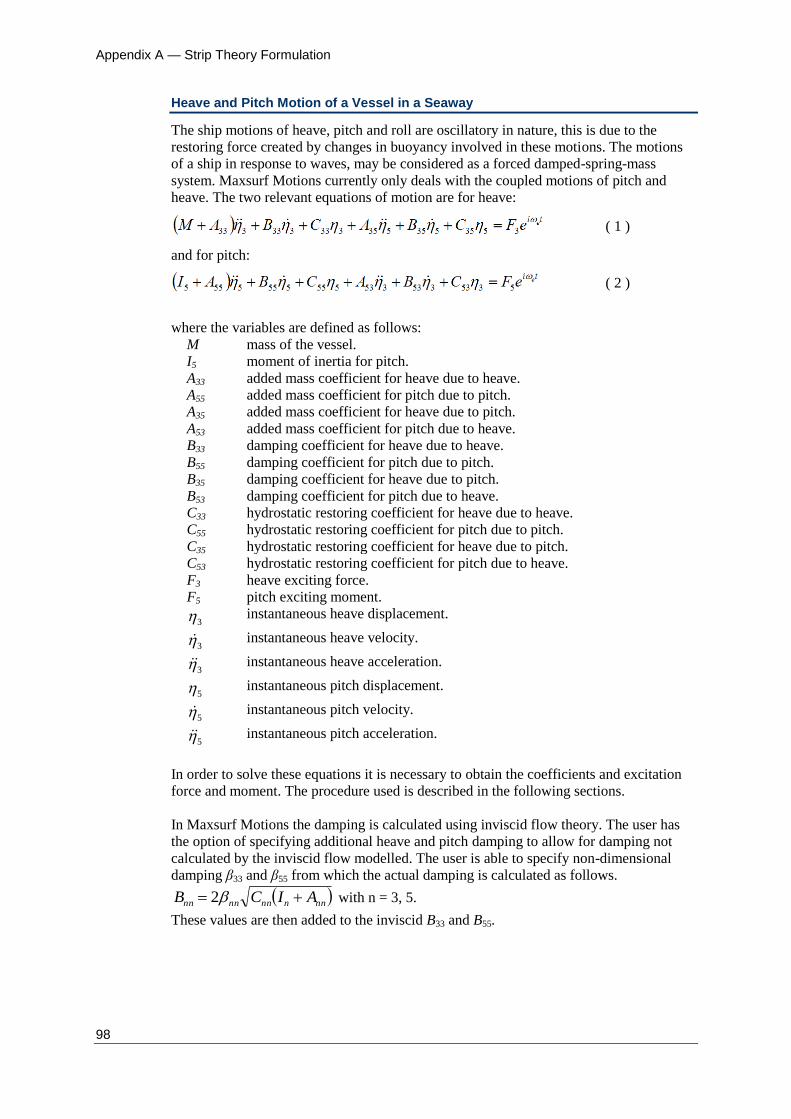
Appendix A — Strip Theory Formulation
98
Heave and Pitch Motion of a Vessel in a Seaway
The ship motions of heave, pitch and roll are oscillatory in nature, this is due to the
restoring force created by changes in buoyancy involved in these motions. The motions
of a ship in response to waves, may be considered as a forced damped-spring-mass
system. Maxsurf Motions currently only deals with the coupled motions of pitch and
heave. The two relevant equations of motion are for heave:
( 1 )
and for pitch:
( 2 )
where the variables are defined as follows:
M mass of the vessel.
I5 moment of inertia for pitch.
A33 added mass coefficient for heave due to heave.
A55 added mass coefficient for pitch due to pitch.
A35 added mass coefficient for heave due to pitch.
A53 added mass coefficient for pitch due to heave.
B33 damping coefficient for heave due to heave.
B55 damping coefficient for pitch due to pitch.
B35 damping coefficient for heave due to pitch.
B53 damping coefficient for pitch due to heave.
C33 hydrostatic restoring coefficient for heave due to heave.
C55 hydrostatic restoring coefficient for pitch due to pitch.
C35 hydrostatic restoring coefficient for heave due to pitch.
C53 hydrostatic restoring coefficient for pitch due to heave.
F3 heave exciting force.
F5 pitch exciting moment.
3 instantaneous heave displacement.
3 instantaneous heave velocity.
3 instantaneous heave acceleration.
5 instantaneous pitch displacement.
5 instantaneous pitch velocity.
5 instantaneous pitch acceleration.
In order to solve these equations it is necessary to obtain the coefficients and excitation
force and moment. The procedure used is described in the following sections.
In Maxsurf Motions the damping is calculated using inviscid flow theory. The user has
the option of specifying additional heave and pitch damping to allow for damping not
calculated by the inviscid flow modelled. The user is able to specify non-dimensional
damping β33 and β55 from which the actual damping is calculated as follows.
nnnnnnnnn AICB 2 with n = 3, 5.
These values are then added to the inviscid B33 and B55.
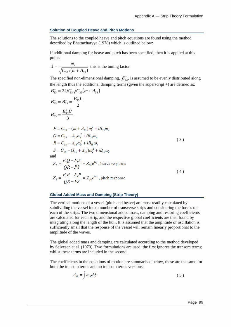
Appendix A — Strip Theory Formulation
Page 99
Solution of Coupled Heave and Pitch Motions
The solutions to the coupled heave and pitch equations are found using the method
described by Bhattacharyya (1978) which is outlined below:
If additional damping for heave and pitch has been specified, then it is applied at this
point.
3333 / AmC
e
this is the tuning factor
The specified non-dimensional damping,
33 , is assumed to be evenly distributed along
the length thus the additional damping terms (given the superscript +) are defined as:
33333333 2 AmCB
2
335335
LBBB
3
2
3355
LBB
( 3 )
and
( 4 )
Global Added Mass and Damping (Strip Theory)
The vertical motions of a vessel (pitch and heave) are most readily calculated by
subdividing the vessel into a number of transverse strips and considering the forces on
each of the strips. The two dimensional added mass, damping and restoring coefficients
are calculated for each strip, and the respective global coefficients are then found by
integrating along the length of the hull. It is assumed that the amplitude of oscillation is
sufficiently small that the response of the vessel will remain linearly proportional to the
amplitude of the waves.
The global added mass and damping are calculated according to the method developed
by Salvesen et al. (1970). Two formulations are used: the first ignores the transom terms;
whilst these terms are included in the second.
The coefficients in the equations of motion are summarised below, these are the same for
both the transom terms and no transom terms versions:
( 5 )

Appendix A — Strip Theory Formulation
100
( 6 )
( 7 )
( 8 )
( 9 )
( 10 )
( 11 )
( 12 )
( 13 )
( 14 )
( 15 )
For the transom terms version, the following terms are added to the coefficients given
above:
( 16 )
( 17 )
( 18 )
( 19 )
( 20 )
( 21 )

Appendix A — Strip Theory Formulation
Page 101
( 22 )
( 23 )
where the variables are defined as follows:
a33 section added mass. Aa33 added mass of transom section.
b33 section damping. Ab33 damping of transom section.
b section beam.
g acceleration due to gravity.
U vessel forward velocity.
xA x ordinate of transom (from CoG, negative aft).
fluid density.
e wave encounter circular frequency.
ζ longitudinal distance from LCB.
The integrals are all over the length of the hull.
Wave Excitation Force and Moment
The wave excitation force and moment drive the motions of the vessel. For solutions of
the coupled heave and pitch equations of motion, only the global force and moment are
required; however, for solution of the wave induced shear force and bending moment, the
forces must be divided into the sectional Froude-Krilov and diffraction forces. Because
several simplifying assumptions may be made, there are three methods available for the
evaluation of the Global Wave Excitation Force and Moment, these are:
Arbitrary wave heading; sectional Froude-Krilov and diffraction forces for arbitrary
wave angles.
Head seas approximation; sectional Froude-Krilov and diffraction forces for head seas.
Salvesen et al. (1970); approximation for global force and moment in head seas.
Again, the methods follow the work of Salvesen et al. (1970).
Arbitrary Wave Heading
This method is used to compute the sectional Froude-Krilov and diffraction forces for
arbitrary wave angles. Other methods, presented below have additional assumptions that
make them simpler and quicker to compute.
Following the work of Salvesen et al. (1970), the global exciting force and moment for
arbitrary wave heading are given by:
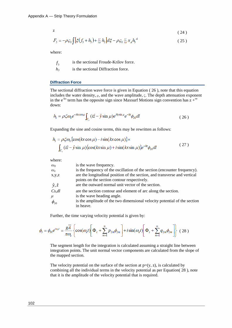
Appendix A — Strip Theory Formulation
102
z ( 24 )
( 25 )
where:
3f is the sectional Froude-Krilov force.
h3 is the sectional Diffraction force.
Diffraction Force
The sectional diffraction wave force is given in Equation ( 26 ), note that this equation
includes the water density, , and the wave amplitude, . The depth attenuation exponent
in the e-kx
term has the opposite sign since Maxsurf Motions sign convention has z +ve
down:
( 26 )
Expanding the sine and cosine terms, this may be rewritten as follows:
( 27 )
where:
ω0 is the wave frequency.
ωe is the frequency of the oscillation of the section (encounter frequency).
x,y,z are the longitudinal position of the section, and transverse and vertical
points on the section contour respectively.
zy ˆ,ˆ are the outward normal unit vector of the section.
Cs,dl are the section contour and element of arc along the section.
μ is the wave heading angle.
30 is the amplitude of the two dimensional velocity potential of the section
in heave.
Further, the time varying velocity potential is given by:
( 28 )
The segment length for the integration is calculated assuming a straight line between
integration points. The unit normal vector components are calculated from the slope of
the mapped section.
The velocity potential on the surface of the section at p=(y, z), is calculated by
combining all the individual terms in the velocity potential as per Equation( 28 ), note
that it is the amplitude of the velocity potential that is required.

Appendix A — Strip Theory Formulation
Page 103
Froude-Krilov Force
The sectional Froude-Krilov wave force is given in Equation ( 29 ), note that this
equation includes the water density, , and the wave amplitude, . Again the depth
attenuation exponent has the opposite sign since Maxsurf Motions sign convention has z
+ve
down (for the 2D section data only):
( 29 )
Expanding the sine and cosine terms, this may be rewritten as follows:
( 30 )
Head Seas Approximation
This method is simplified by assuming that the vessel is in head seas. The sectional
Froude-Krilov and diffraction forces are obtained which makes this method suitable for
the loads calculations.
The head seas approximation to the sectional Froude-Krilov wave force is given in
Equation ( 31 ), note that this equation includes the water density, , and the wave
amplitude, . This follows the work of Salvesen et al. (1970), Equations STF-32, 33
( 31 )
Expanding the sine and cosine terms, this may be rewritten as follows:
( 32 )
where:
b is the total section beam.
d is the section draft.
As is the section area.
is the section area coefficient. Note that
b
Ads s .
Secondly, the head seas approximation to the sectional diffraction wave force is given in
Equation ( 33 ), note that this equation includes the water density, , and the wave
amplitude, :
( 33 )
Expanding the sine and cosine terms, this may be rewritten as follows:
( 34 )
where:
a33 is the section added mass in heave.
b33 is the section damping in heave.
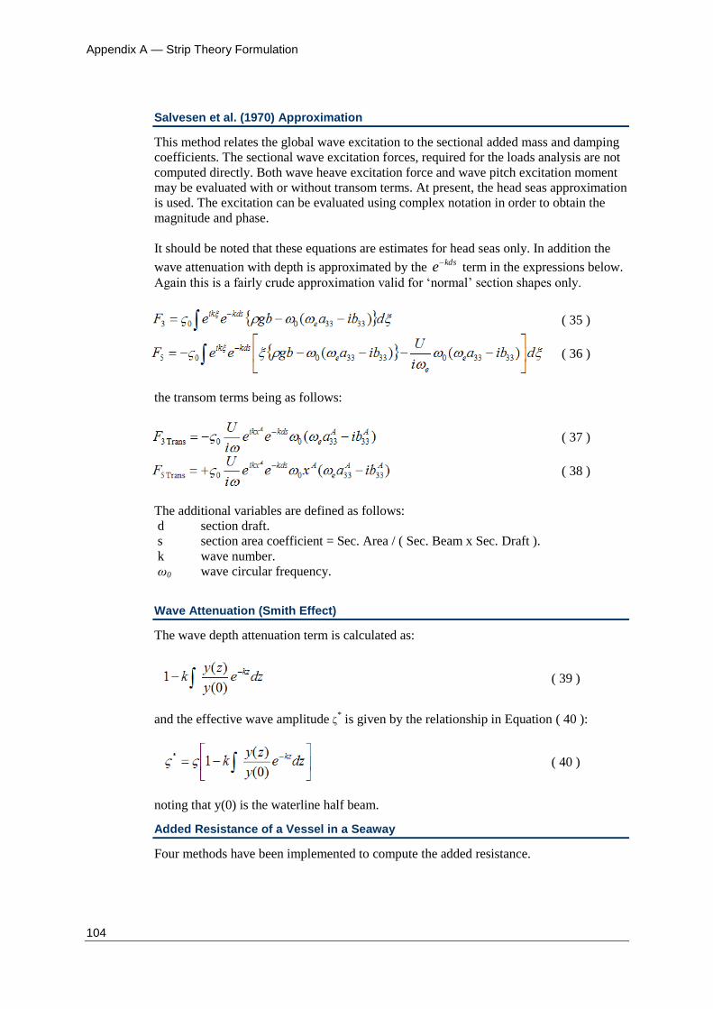
Appendix A — Strip Theory Formulation
104
Salvesen et al. (1970) Approximation
This method relates the global wave excitation to the sectional added mass and damping
coefficients. The sectional wave excitation forces, required for the loads analysis are not
computed directly. Both wave heave excitation force and wave pitch excitation moment
may be evaluated with or without transom terms. At present, the head seas approximation
is used. The excitation can be evaluated using complex notation in order to obtain the
magnitude and phase.
It should be noted that these equations are estimates for head seas only. In addition the
wave attenuation with depth is approximated by the kdse
term in the expressions below.
Again this is a fairly crude approximation valid for ‘normal’ section shapes only.
( 35 )
( 36 )
the transom terms being as follows:
( 37 )
( 38 )
The additional variables are defined as follows:
d section draft.
s section area coefficient = Sec. Area / ( Sec. Beam x Sec. Draft ).
k wave number.
ω0 wave circular frequency.
Wave Attenuation (Smith Effect)
The wave depth attenuation term is calculated as:
( 39 )
and the effective wave amplitude * is given by the relationship in Equation ( 40 ):
( 40 )
noting that y(0) is the waterline half beam.
Added Resistance of a Vessel in a Seaway
Four methods have been implemented to compute the added resistance.

Appendix A — Strip Theory Formulation
Page 105
Gerritsma and Beukelman
The first two are based on the work of Gerritsma and Beukelman (1972). The added
resistance is related to the relative vertical velocity of the vessel compared with the wave
surface and the damping coefficient. The difference between the two versions is a small
difference in the expression for the relative vertical motion. The general formulation is
given in the following equation:
( 41 )
where d
d 3333
*
33
aUbb is a modified section damping; and
2
zaV is the relative vertical
velocity, given by Equation ( 42 ).
( 42 )
where * is given by Equation ( 43 ).
Note that 3, 3 and * are the complex heave, pitch and local relative wave amplitudes,
containing both phase and amplitude information.
The two methods vary only in the expression for the derivative of * . Version A uses the
expression in Equation ( 43 ), whilst Version B uses the expression in
Equation ( 44 ).
( 43 )
( 44 )
Salvesen
In the third method, described by Salvesen (1978), the added resistance is given by
Equation ( 45 ).
( 45 )
where
and
Note that 3 and 3 are the complex heave and pitch amplitudes, containing both phase
and amplitude information.

Appendix A — Strip Theory Formulation
106
Havelock
Finally the added resistance using a method proposed by Havelock (1942) is given by:
5553332sinsin FFR k
AW ( 46 )
Where F3 and F5 are the magnitudes of the heave and pitch excitation force and moment;
µ3 and µ 5 are the magnitudes of the heave and pitch motions; and
ε3 and ε 5 are the phase differences of the heave and pitch motions with the corresponding
excitation force or moment.
2D Ship Sections
The calculation of the added mass and damping of two dimensional ship sections, is
based on the work of Ursell (1949), for a two-dimensional circular cylinder heaving in
the free surface. The work of Bishop et al. (1978) has expanded the original approach to
include conformal mapping techniques which may be used to map the ship’s section to a
unit circle centred at the origin, and hence calculate the hydrodynamic coefficients of
arbitrary ship sections. The work of Sutherland (1987) is also a useful starting point and
rephrases the method of Bishop et al. (1977).
Calculation of Added Mass and Damping of 2D Ship Sections
The conformal mappings are described in greater detail in section Conformal Mapping
on page 10, but the general form of the mapping equation is given below in
Equation ( 47 ).
( 47 )
The work of Ursell (1949) develops a formulation for the added mass and damping of a
heaving circular cylinder in a free surface. The presence of the free surface gives rise to
the frequency dependence of the hydrodynamic coefficients. Ursell used a multipole
expansion of the stream function and velocity potential to determine the flow around the
cylinder, and hence derive the hydrodynamic coefficients.
The principle steps of the method are given in the following sections.
Calculation of multipole expansion coefficients
As mentioned above, the stream function and velocity potential are expressed as
multipole expansions. The coefficients of the multipole expansion, p2m and q2m, are found
by applying the appropriate boundary condition at the cylinder surface. This leads to
Equation ( 48 ).
( 48 )
This may be re-arranged and expressed in matrix form:
Ax = b ( 49 )
Where the vector x contains the p2m or q2m terms, the matrix A contains the f2m terms and
the vector b contains the c or s terms.

Appendix A — Strip Theory Formulation
Page 107
The terms in Equation ( 48 ) are evaluated as follows:
( 50 )
( 51 )
( 52 )
The mapped points y, z are obtained by applying the mapping equation at angle
(Equation( 50 )).
Since the integral in Equation ( 52 ) converges slowly it is evaluated by an alternative
method. The method used follows the work of Sutherland and is known as the method of
Laguerre-Gauss quadrature. It may be shown that the integral can be evaluated as in
Equation ( 53 ):
( 53 )
Where the weighting functions, wi, and the abscissa, si, may be found in standard texts.
Finally the f2m terms are calculated for each multipole at each angle according to
Equation ( 54 ):
( 54 )
with 2m:
( 55 )
where a0, a1, ... aN are the conformal mapping coefficients.
Least squares solution to over-defined set of linear equations
In practice, Equation ( 49 ) is solved in a least squares sense: a number of angles, R, are
chosen at which the c and s terms are evaluated from Equations ( 51 ) and ( 52 ). The
number of multipoles, M, is chosen such that M < R, and the f2m terms are evaluated,
according to Equation ( 54 ), for each of the multipoles at each of the angles. Thus there
are more linear equations than unknowns. It may be shown that the least squares solution
to this system of equations may be expressed, in matrix form, as in Equation ( 51 ). This
system may then easily be solved by Gauss elimination or any other matrix solving
method, such as Gauss Seidel or SOR (successive over-relaxation).

Appendix A — Strip Theory Formulation
108
ATAx = A
T b ( 56 )
Calculation and integration of pressure functions around contour
Once the coefficients, p2m and q2m, have been found, it is necessary to calculate the terms
M0 and N0. These are calculated according to Equation ( 57 ), where the functions are
integrated over one quadrant of the section in the unit circle plane.
( 57 )
The terms M(), N() and W() are given in Equations ( 58 ):
( 58 )
The terms s, c and 2m are calculated from Equations ( 59 ):
( 59 )
Again the integral in the s term is evaluated by Laguerre quadrature using
Equation ( 60 ):
( 60 )
Additional terms A and B are calculated from Equation ( 61 ):
( 61 )
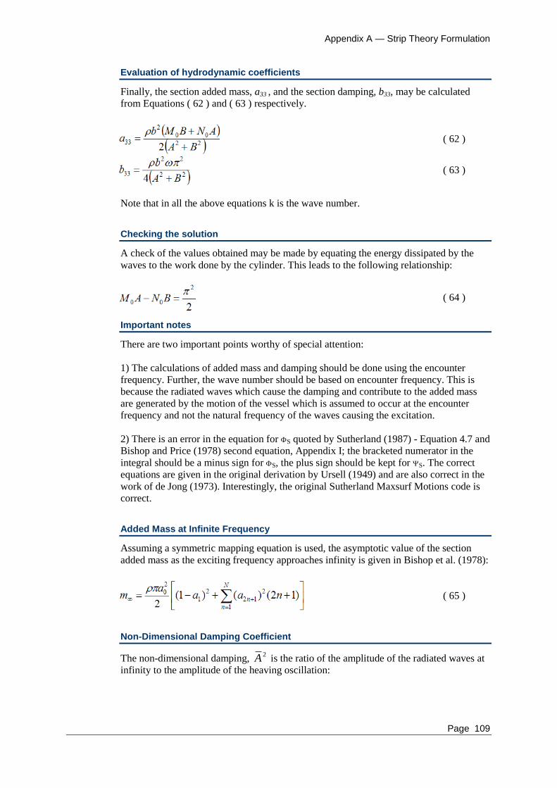
Appendix A — Strip Theory Formulation
Page 109
Evaluation of hydrodynamic coefficients
Finally, the section added mass, a33 , and the section damping, b33, may be calculated
from Equations ( 62 ) and ( 63 ) respectively.
( 62 )
( 63 )
Note that in all the above equations k is the wave number.
Checking the solution
A check of the values obtained may be made by equating the energy dissipated by the
waves to the work done by the cylinder. This leads to the following relationship:
( 64 )
Important notes
There are two important points worthy of special attention:
1) The calculations of added mass and damping should be done using the encounter
frequency. Further, the wave number should be based on encounter frequency. This is
because the radiated waves which cause the damping and contribute to the added mass
are generated by the motion of the vessel which is assumed to occur at the encounter
frequency and not the natural frequency of the waves causing the excitation.
2) There is an error in the equation for S quoted by Sutherland (1987) - Equation 4.7 and
Bishop and Price (1978) second equation, Appendix I; the bracketed numerator in the
integral should be a minus sign for S, the plus sign should be kept for S. The correct
equations are given in the original derivation by Ursell (1949) and are also correct in the
work of de Jong (1973). Interestingly, the original Sutherland Maxsurf Motions code is
correct.
Added Mass at Infinite Frequency
Assuming a symmetric mapping equation is used, the asymptotic value of the section
added mass as the exciting frequency approaches infinity is given in Bishop et al. (1978):
( 65 )
Non-Dimensional Damping Coefficient
The non-dimensional damping, 2A is the ratio of the amplitude of the radiated waves at
infinity to the amplitude of the heaving oscillation:
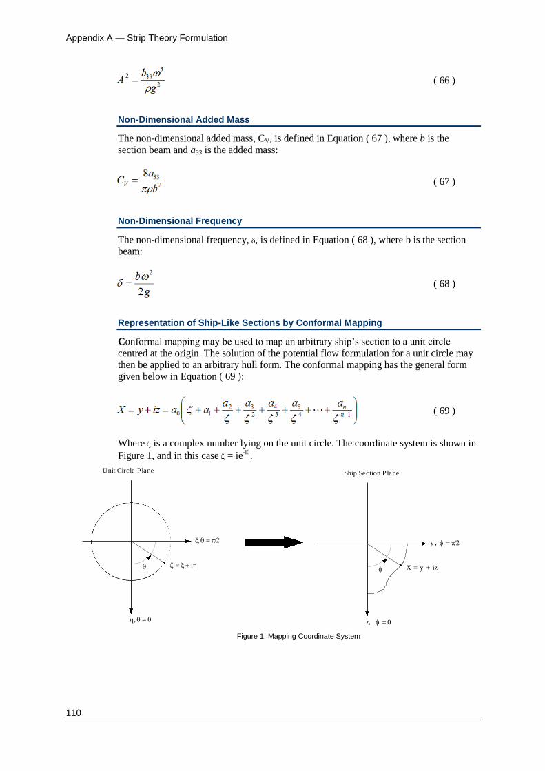
Appendix A — Strip Theory Formulation
110
( 66 )
Non-Dimensional Added Mass
The non-dimensional added mass, CV, is defined in Equation ( 67 ), where b is the
section beam and a33 is the added mass:
( 67 )
Non-Dimensional Frequency
The non-dimensional frequency, , is defined in Equation ( 68 ), where b is the section
beam:
( 68 )
Representation of Ship-Like Sections by Conformal Mapping
Conformal mapping may be used to map an arbitrary ship’s section to a unit circle
centred at the origin. The solution of the potential flow formulation for a unit circle may
then be applied to an arbitrary hull form. The conformal mapping has the general form
given below in Equation ( 69 ):
( 69 )
Where is a complex number lying on the unit circle. The coordinate system is shown in
Figure 1, and in this case = ie-i
.
X = y + iz
Unit Circle Plane Ship Section Plane
z,
y ,
i
Figure 1: Mapping Coordinate System
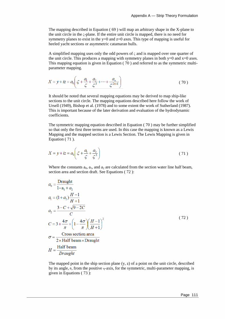
Appendix A — Strip Theory Formulation
Page 111
The mapping described in Equation ( 69 ) will map an arbitrary shape in the X-plane to
the unit circle in the -plane. If the entire unit circle is mapped, there is no need for
symmetry planes to exist in the y=0 and z=0 axes. This type of mapping is useful for
heeled yacht sections or asymmetric catamaran hulls.
A simplified mapping uses only the odd powers of and is mapped over one quarter of
the unit circle. This produces a mapping with symmetry planes in both y=0 and x=0 axes.
This mapping equation is given in Equation ( 70 ) and referred to as the symmetric multi-
parameter mapping.
( 70 )
It should be noted that several mapping equations may be derived to map ship-like
sections to the unit circle. The mapping equations described here follow the work of
Ursell (1949), Bishop et al. (1978) and to some extent the work of Sutherland (1987).
This is important because of the later derivation and evaluation of the hydrodynamic
coefficients.
The symmetric mapping equation described in Equation ( 70 ) may be further simplified
so that only the first three terms are used. In this case the mapping is known as a Lewis
Mapping and the mapped section is a Lewis Section. The Lewis Mapping is given in
Equation ( 71 ).
( 71 )
Where the constants a0, a1, and a2 are calculated from the section water line half beam,
section area and section draft. See Equations ( 72 ):
( 72 )
The mapped point in the ship section plane (y, z) of a point on the unit circle, described
by its angle, , from the positive -axis, for the symmetric, multi-parameter mapping, is
given in Equations ( 73 ):
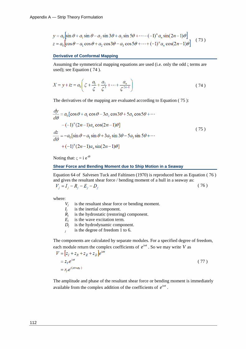
Appendix A — Strip Theory Formulation
112
( 73 )
Derivative of Conformal Mapping
Assuming the symmetrical mapping equations are used (i.e. only the odd terms are
used); see Equation ( 74 ).
( 74 )
The derivatives of the mapping are evaluated according to Equation ( 75 ):
( 75 )
Noting that: = i e-i
Shear Force and Bending Moment due to Ship Motion in a Seaway
Equation 64 of Salvesen Tuck and Faltinsen (1970) is reproduced here as Equation ( 76 )
and gives the resultant shear force / bending moment of a hull in a seaway as:
( 76 )
where:
Vj is the resultant shear force or bending moment.
Ij is the inertial component.
Rj is the hydrostatic (restoring) component.
Ej is the wave excitation term.
Dj is the hydrodynamic component.
j is the degree of freedom 1 to 6.
The components are calculated by separate modules. For a specified degree of freedom,
each module return the complex coefficients of tie . So we may write V as
( 77 )
The amplitude and phase of the resultant shear force or bending moment is immediately
available from the complex addition of the coefficients of tie .

Appendix A — Strip Theory Formulation
Page 113
Inertial Component
This module calculates the vertical shear forces and bending moment components due to
the inertial forces.
The section inertial loading in heave, i3, is given by Equation ( 78 ) (Salvesen et al. 1970,
Equation 66):
( 78 )
The shear force at section x0 is calculated by integrating the loading forward of the
section of interest. Thus the shear force due to the inertial forces is given by:
( 79 )
The bending moment at section x0 is given by Salvesen et al. 1970, Equation 68:
( 80 )
where i5 is given by:
( 81 )
m section mass per unit length.
η3 heave response.
η5 pitch response.
ω encounter frequency.
ξ longitudinal distance from LCG.
x0 longitudinal position of section of interest.
The functions in this module are set up to calculate the value of the integrands at all
sections and then integrate over the appropriate sections to obtain the shear force and
bending moments; integrations are evaluated using the trapezium rule.
The bending moment integrands are dependent on the section, x0, at which the bending
moment is being evaluated and hence need to be re-evaluated for each section.
Hydrostatic (Restoring) Component
This module calculates the vertical shear forces and bending moment components due to
the hydrostatic restoring forces.
The section hydrostatic restoring loading in heave, r3, is given by (Salvesen et al. 1970,
Equation 70):
( 82 )
The shear force at section x0 is calculated by integrating the loading forward of the
section of interest. Thus the shear force due to the hydrostatic restoring force is given by:
( 83 )
The bending moment at section x0 is given by (Salvesen et al. 1970, Equation 68):
( 84 )
where r5 is given by:
( 85 )
Appendix A — Strip Theory Formulation
114
b section waterline beam.
η3 heave response.
η5 pitch response.
ω encounter frequency.
ξ longitudinal distance from LCG.
x0 longitudinal position of section of interest.
The functions in this module are set up to calculate the value of the integrands at all
sections and then integrate over the appropriate sections to obtain the shear force and
bending moments; integrations are evaluated using the trapezium rule. The bending
moment integrands are dependent on the section, x0, at which the bending moment is
being evaluated and hence need to be re-evaluated for each section.
Wave Excitation Component
This module calculates the vertical shear forces and bending moment components due to
the incident wave excitation forces.
The section wave excitation loading in heave, e3, is given by (Salvesen et al. 1970,
Equation 73):
( 86 )
Here the Froude-Krilov force, f3, and the wave diffraction force, h3, as calculated in the
hydrodynamics module, include the wave amplitude and water density factor .
The shear force at section x0 is calculated by integrating the loading forward of the
section of interest and adding a speed dependent term. Thus the shear force due to the
wave excitation is given by:
( 87 )
The bending moment at section x0 is given by (Salvesen et al. 1970, Equation 74):
( 88 )
where e5 is given by:
( 89 )
f3 2D section Froude-Krilov wave force in heave.
h3 2D section diffraction wave force in heave.
ω encounter frequency.
ξ longitudinal distance from LCG.
x0 longitudinal position of section of interest.
The functions in this module are set up to calculate the value of the integrands at all
sections and then integrate over the appropriate sections to obtain the shear force and
bending moments; integrations are evaluated using the trapezium rule.
The bending moment integrands are dependent on the section, x0, at which the bending
moment is being evaluated and hence need to be re-evaluated for each section.
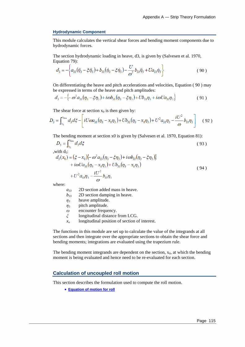
Appendix A — Strip Theory Formulation
Page 115
Hydrodynamic Component
This module calculates the vertical shear forces and bending moment components due to
hydrodynamic forces.
The section hydrodynamic loading in heave, d3, is given by (Salvesen et al. 1970,
Equation 79):
( 90 )
On differentiating the heave and pitch accelerations and velocities, Equation ( 90 ) may
be expressed in terms of the heave and pitch amplitudes:
( 91 )
The shear force at section x0 is then given by:
( 92 )
The bending moment at section x0 is given by (Salvesen et al. 1970, Equation 81):
( 93 )
,with d5:
( 94 )
where:
a33 2D section added mass in heave.
b33 2D section damping in heave.
η3 heave amplitude.
η5 pitch amplitude.
ω encounter frequency.
ξ longitudinal distance from LCG.
xo longitudinal position of section of interest.
The functions in this module are set up to calculate the value of the integrands at all
sections and then integrate over the appropriate sections to obtain the shear force and
bending moments; integrations are evaluated using the trapezium rule.
The bending moment integrands are dependent on the section, x0, at which the bending
moment is being evaluated and hence need to be re-evaluated for each section.
Calculation of uncoupled roll motion
This section describes the formulation used to compute the roll motion.
Equation of motion for roll

Appendix A — Strip Theory Formulation
116
Equation of motion for roll
The vessel's roll motion may be represented by a second order differential equation, such
as that describing a forced spring, mass and damper system.
( 95 )
where the variables are defined as follows:
I4 moment of inertia for roll.
A44 added inertia coefficient for roll.
B44 damping coefficient for roll.
C44 hydrostatic restoring coefficient for roll.
F4 roll exciting moment at the encounter frequency e .
η4 instantaneous roll displacement.
4 instantaneous roll velocity.
4 instantaneous roll acceleration.
It may be shown that the solution to the above equation is given by:
where: is the phase lag relative to the forcing function: 2
44444
44tane
e
AIC
B
This equation may be re-expressed in terms of the damping ratio,
44444
4444
2 AIC
B
, the natural frequency of the system,
444
440
AI
C
, and
the tuning factor, 0
e .
As an aside, it may be shown (by differentiation of the RAO function) that the damped
natural frequency is given by:
2
00 21 damped
The roll transfer function or response function is then assumed to be given by:
Strictly speaking this is the roll motion transfer function with regard to wave force and
not wave slope, however, the two are assumed to be the same.
The RAO is then modified for wave heading and apparent wave slope so that the RAO at
off head seas is given by:
thus the roll RAO is zero in head and following seas and has a maximum in beam seas.

Appendix A — Strip Theory Formulation
Page 117
In Maxsurf Motions the required parameters are determined as follows:
I4 mass inertia of vessel in roll 2
4 xxkI , xxk input by user
A44 added inertia coefficient for roll 444 3.0 IA , this is an average of values
from Vugts (1968) and Lloyd (1998)
β44 Non-dimensional damping coefficient for roll, input by user.
C44 hydrostatic restoring coefficient for roll gGMC t 44 , VCG input by
user
Roll free-decay test
If experimental facilities are available, the roll damping can be obtained from a free-
decay test of the roll motions. The vessel is heeled over to one side and released, the roll
amplitude is measured and plotted against time. The figure below shows the theoretical
free-decay of two vessels with different damping coefficients.
Free-decay time series for two vessels released from an initial heel angle of 30 degrees
By plotting the value of one peak against the value of the next peak (the same can also be
done for the troughs to obtain more data), the roll damping can be derived.
Peak/trough amplitudes for beta 0.075 vessel
beta0.075 peak/trough i peak/trough i+1
trough 1 30.000 18.755
peak 1 23.752 14.808
trough 2 18.755 11.692
peak 2 14.808 9.231
trough 3 11.692 7.289
peak 3 9.231 5.754
trough 4 7.289 4.544
peak 4 5.754
trough 5 4.544

Appendix A — Strip Theory Formulation
118
Peak/trough amplitudes for beta 0.1 vessel
beta0.1 peak/trough i peak/trough i+1
trough 1 30.000 16.001
peak 1 21.745 11.646
trough 2 16.001 8.519
peak 2 11.646 6.183
trough 3 8.519 4.518
peak 3 6.183 3.285
trough 4 4.518 2.405
peak 4 3.285 1.747
trough 5 2.405 1.279
peak 5 1.747
trough 6 1.279
Plot of peak amplitude against peak amplitude of next peak. In this example, data for both peaks and troughs have been plotted
The non-dimensional roll damping parameter used in Maxsurf Motions, β44, is given by:
2
)slopeln(44
Thus for the beta0.075 vessel, the slope is 1.6023, giving a damping of 0.075 (as
expected); similarly for the beta0.1 vessel, the slope is 1.8747 giving a damping of 0.100.
The free-decay roll test can be simulated in Maxsurf Motions by choosing Roll decay
simulation option in the Analysis | Calculate Wave Surface dialog, then choosing Display
| Animate and saving the time-series to a file:

Appendix A — Strip Theory Formulation
Page 119
Simulation of free-decay roll test in Maxsurf Motions


Appendix B — Validation
Page 121
Appendix B Strip theory validation
Maxsurf Motions has been validated against various sources of public data.
Maxsurf Motions Validation 1 – NPL Round Bilge series
Maxsurf Motions Validation 2 – Series 60
Maxsurf Motions Validation 3 – SA van der Stel
The numerical calculation routines and algorithms for the two dimensional section
hydrodynamic coefficients have been validated against calculations for standard sections,
e.g. Bishop and Price (1979).
In addition the heave and pitch response, predicted by Maxsurf Motions, has been
validated against several sources of experimental data from both model scale and full
size vessels: e.g. Molland et al. (1995) and data obtained by AMECRC for various full
scale vessels and model yachts tests.
Maxsurf Motions Validation 1 – NPL Round Bilge series
Use of Maxsurf Motions for predicting the heave and pitch response of high-speed
catamaran and monohull hullforms based on NPL Round Bilge series.
Introduction
This document forms part of the validation of Formation Design Systems' seakeeping
software Maxsurf Motions. The Maxsurf Motions program is fully integrated into the
Maxsurf naval architecture design suite.
Maxsurf Motions uses Strip Theory (Salvesen et al. 1970) to predict the heave and pitch
response of a vessel in a seaway. Conformal mapping methods and inviscid flow
calculations are used to compute the section added mass and damping.
Calculations are presented for a standard series of catamaran forms tested at the
University of Southampton (Molland et al. 1995, Couser 1996). The results from
Maxsurf Motions are compared with those from towing tank measurements for three
Length:Displacement ratios, two demihull separations (and single demihull in isolation)
for three different speeds. The hullforms tested were based on the NPL round bilge series
(Bailey 1976) see Figure 1; the hulls having been stretched in the longitudinal direction
to give suitable Length:Displacement ratios. A summary of the test conditions is given
below:
Model principal particulars
Name Hullform L/1/3
L/B B/T LBP
4b NPL r/b 7.4 9 2 1.6m
5b NPL r/b 8.5 11 2 1.6m
6b NPL r/b 9.5 13 2 2.1m
Separations tested: S/L = 0.2, 0.4, Monohull
Speeds tested: Fn = 0.20, 0.53, 0.80.
Tank Dimensions
Length 60.0m
Breadth 3.7m
Water depth 1.85m

Appendix B – Validation
122
Max. carriage speed 4.6m/s
All tests were conducted in head seas.
Analysis Procedure
The Maxsurf Motions analysis was carried out using 41 equally spaced sections to define
the hull and 3 parameter Lewis mappings were used to compute the section
hydrodynamic properties. In all cases the basic inviscid Salvesen et al. (1970) Strip
Theory formulation was used with no additional damping terms; for the high Froude
numbers, the analysis was also performed including the Salvesen et al. (1970) transom
stern correction.
The computed RAOs (magnitude and phase) are compared with those from the tank tests
in regular waves. In all cases, heave has been non-dimensionalised against wave height
and pitch against wave slope. The phase lag between the motion and the wave at the
centre of gravity is given in degrees.
A comparison of the hullform and the mapped Lewis sections is given in Figure 1. It may
be seen that the mappings give a reasonable definition of the actual surface, though there
is scope for improvement of the mapping by using more mapping terms.
The motions of the catamaran have been predicted by computing the motions of a single
demihull in isolation. For all but the lowest speeds the interaction between the demihulls
is small, particularly for the wider spacing of , Separation:Length ratio, S/L = 0.4.
Results
The results are presented in Figures 2 to 10. For each of the figures, Figure a is the heave
RAO; Figure b is the heave phase; Figure c the pitch RAO and Figure d the pitch phase.
The Maxsurf Motions results are for a single demihull in isolation. These have been
compared with the towing tank data for the two catamaran configurations and the
demihull tested in isolation (monohull). It may be seen that for all but the lowest speeds,
the interaction between the two catamaran demihulls is small.
Slow Speed
Figures 2 to 4 give the results for model 4b; Figures 5 to 7 those for model 5b and
Figures 8 to 10 those for the most slender model, 6b.
For the slowest Froude number (Fn = 0.20), Figures 2, 5 and 8, the Maxsurf Motions
results show good correlation with the monohull model tests, for all the
Length:Displacement ratios. The interaction between the demihulls, which may be
observed as a secondary resonant peak is not computed since the Maxsurf Motions model
is for a single demihull in isolation. However, these secondary resonant peaks diminish
rapidly with increasing Length:Displacement ratio (going from model 4b to 6b); and
excellent correlation is found for model 6b for both catamaran configurations.

Appendix B — Validation
Page 123
Moderate Speed
At moderate Froude number, Maxsurf Motions results have been computed with and
without additional transom terms. These terms significantly increase the damping,
particularly for pitch. The terms are suggested by Salvesen et al. (1970) because the Strip
Theory formulation assumes that the sectional added mass and damping tend to zero at
the vessel bow and stern. However, for high-speed semi-displacement forms which have
transom areas which are often a large proportion of the maximum cross sectional area, it
is felt, that the transom terms provide an excessive amount of extra damping and some
judgement, on the part of the designer, is required to determine whether transom terms
should be included or not.
For heave at Froude number = 0.53, Figures 3, 6 and 9, Maxsurf Motions predictions
including transom terms are closest to the experiment results. However, for pitch, results
without transom terms are more accurate. In all cases the Maxsurf Motions predictions
show good correlation with the experiment results for the two catamaran configurations.
The experimental results for the demihull in isolation (monohull) are slightly reduced
when compared with those of the two catamaran configurations.
Maxsurf Motions tends to over predict the frequency at which the resonant peak occurs,
and this is more so for the predictions of pitch response. As might be expected, the
discrepancies between predictions and experiments reduce for the more slender models
(going from model 4b to 6b). However, in general the predictions at Fn = 0.53 are quite
reasonable.
High Speed
At the highest Froude number tested (Fn = 0.80), Figures 4, 7 and 10, Maxsurf Motions
predictions start to over predict the heave response if transom terms are not included. If
transom terms are included good estimates of the peak response are achieved. However,
the difference between the predicted and measured resonant frequencies is increased
when compared with the results at slower Froude numbers.
Predictions of the pitch response with and without transom terms show significant
differences, and this is due to the velocity term in the transom terms. Again, the
magnitude of the resonant peak is relatively well predicted when transom terms are
included but the frequency at which the peak occurs is poorly predicted.
Conclusions
Maxsurf Motions predictions for the heave and pitch response to regular head waves
have been compared with towing tank results for a number of geometrically similar
hullforms of differing length: displacement ratio at three different speeds; Fn = 0.20,
0.53, 0.80. For the hullforms tested (based on the NPL round bilge series, Bailey 1976)
Maxsurf Motions was able to adequately predict the heave and pitch response up to a
Froude number of 0.53; predictions at higher speeds suffered from poor prediction of the
resonant frequency, although the magnitude of the resonant peak was reasonably well
calculated.
Catamaran results were obtained from Maxsurf Motions by modelling a single demihull
in isolation. Experiments show that the differences between the catamaran and isolated
demihull configurations are most pronounced at slow Froude numbers (Fn = 0.20) and for
catamarans with closely spaced demihulls and small length: displacement ratios.

Appendix B – Validation
124
References
Bailey, D. 1967. The NPL high speed round bilge displacement hull series. Maritime
Technology Monograph No. 4, Royal Institution of Naval Architects.
Couser, P.R. 1996. An investigation into the performance of high-speed catamarans in
calm water and waves. PhD thesis, University of Southampton, March.
Molland, A.F., Wellicome, J.F. and Couser, P.R. 1995. Experimental measurements of
the seakeeping characteristics of fast displacement catamarans in long-crested head-
seas. University of Southampton, Ship Science Report No. 89, December.
Salvesen, N., Tuck, O.E. and Faltinsen, O., 1970. Ship motions and sea loads.
Transactions, Society of Naval Architects and Marine Engineers, No. 78, pp250-287.
Figures
Figure 1: NPL hullform with Lewis sections used for seakeeping analysis

Appendix B — Validation
Page 125
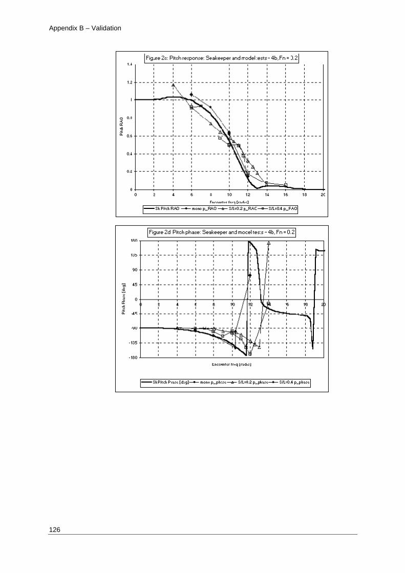
Appendix B – Validation
126

Appendix B — Validation
Page 127

Appendix B – Validation
128

Appendix B — Validation
Page 129
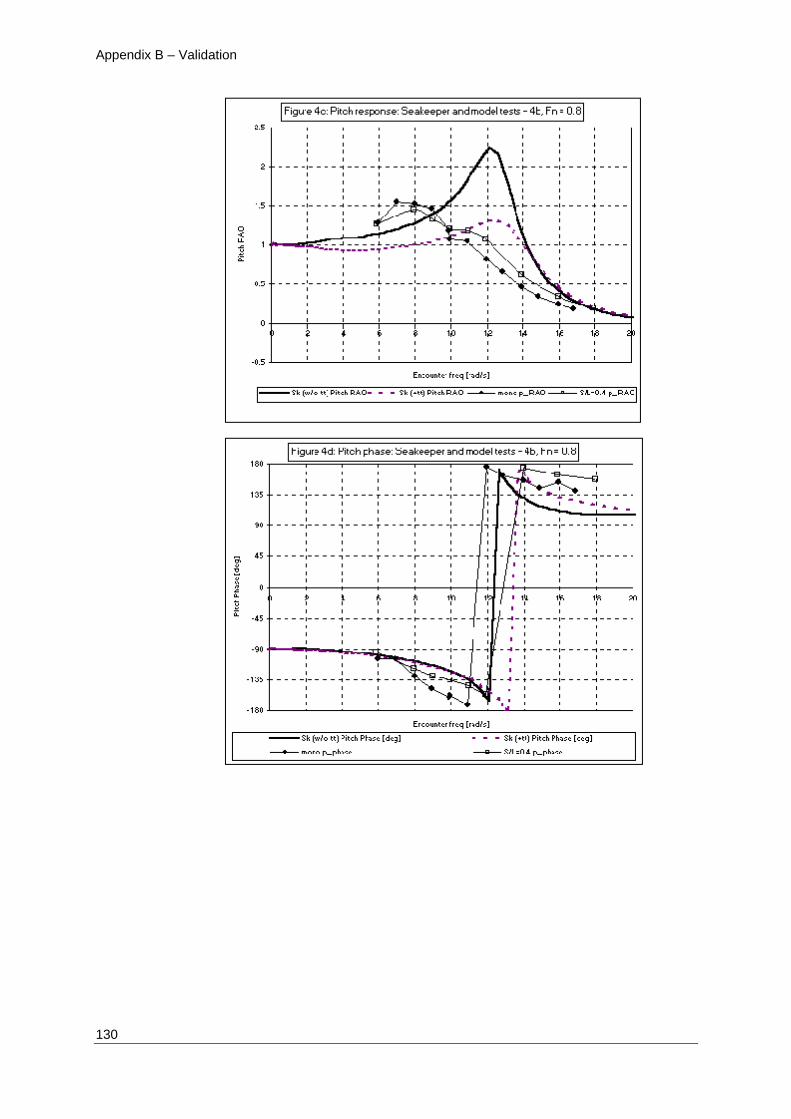
Appendix B – Validation
130

Appendix B — Validation
Page 131
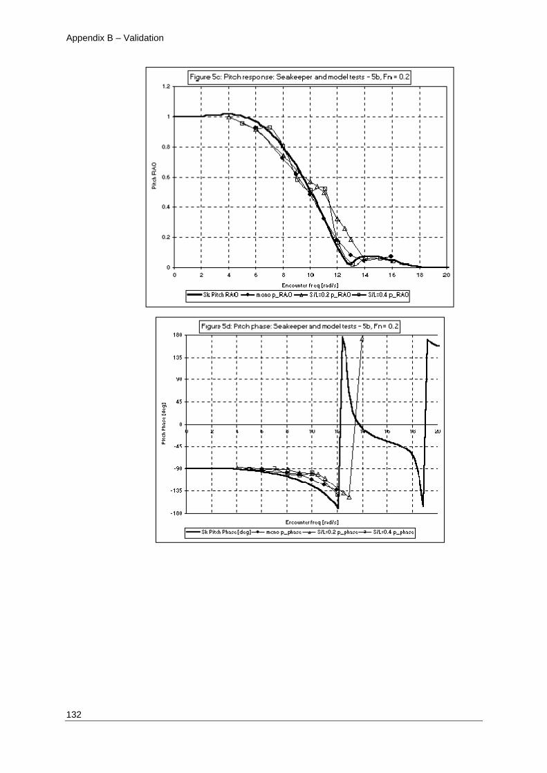
Appendix B – Validation
132

Appendix B — Validation
Page 133
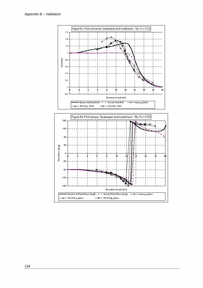
Appendix B – Validation
134

Appendix B — Validation
Page 135

Appendix B – Validation
136

Appendix B — Validation
Page 137
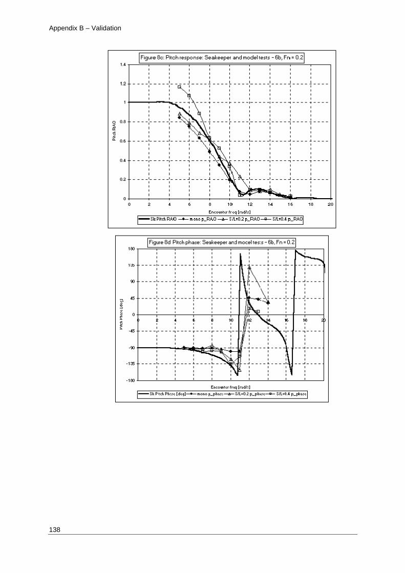
Appendix B – Validation
138
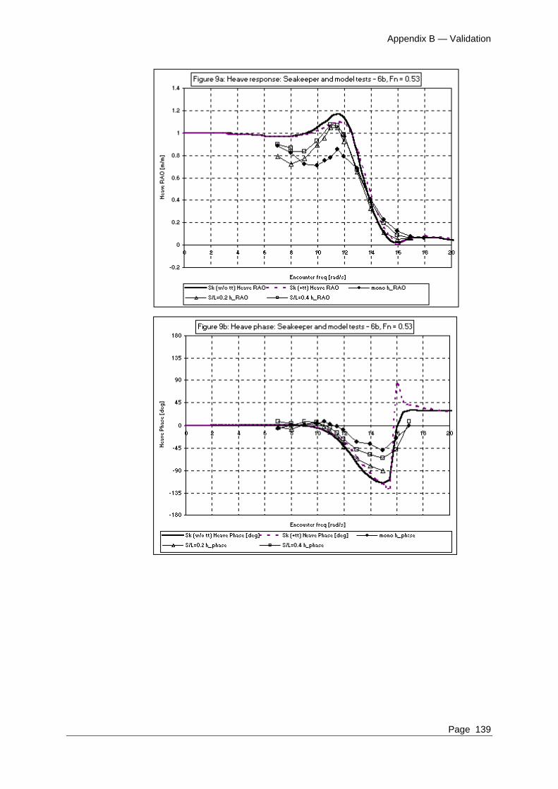
Appendix B — Validation
Page 139
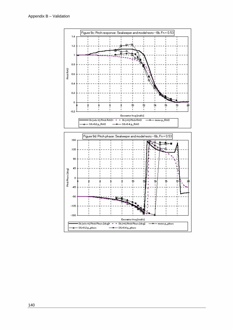
Appendix B – Validation
140
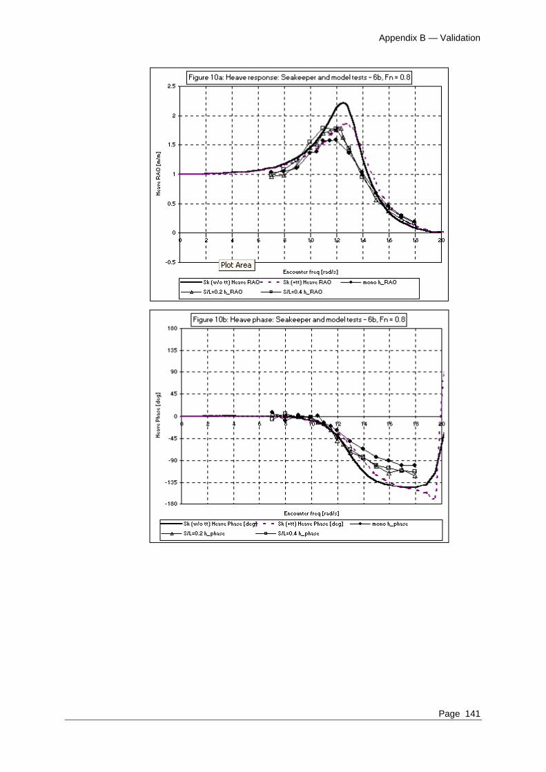
Appendix B — Validation
Page 141

Appendix B – Validation
142
Maxsurf Motions Validation 2 – Series 60
Use of Maxsurf Motions for predicting the heave and pitch response of the Series 60
CB=0.7 hullform – Comparison with SWAN and experiments.
Introduction
This document forms part of the validation of Formation Design Systems' seakeeping
software Maxsurf Motions. The Maxsurf Motions software is fully integrated into the
Maxsurf naval architecture design suite.

Appendix B — Validation
Page 143
Maxsurf Motions uses Strip Theory (Salvesen et al. 1970) to predict the heave and pitch
response of a vessel in a seaway. Conformal mapping methods and inviscid flow
calculations are used to compute the section added mass and damping.
Calculations are presented for the standard Series 60, CB=0.7, hullform. This vessel has
been the subject of many theoretical and experimental investigations over a number of
years. The results from Maxsurf Motions are compared with those from towing tank
measurements (Gerritsma 1960; Gerritsma and Beukelman 1966) and also for a non-
linear time domain program developed at MIT – SWAN (Sclavounos et al. 1997).
Results for two speeds, Fn = 0.2 and 0.3, are presented.
Hullform principal particulars
Hullform L/
1/3 L/B B/T LBP
Series 60, CB=0.7 5.6 7.0 2.5 101.7m
Speeds tested: Fn = 0.2, 0.3. All tests were done in head seas. The model tested by
Gerritsma (1960) was 2.438m in length.
Analysis Procedure
The Maxsurf Motions analysis was carried out using 41 equally spaced sections to define
the hull and 3 parameter Lewis mappings were used to compute the section
hydrodynamic properties. In all cases the basic inviscid Salvesen et al. (1970) Strip
Theory formulation was used with no additional damping terms; transom terms were not
included. The hullform is shown in Figure 1.
Results
Froude number = 0.2
The heave response at Fn = 0.2 is given in Figure 4a and the pitch response in Figure 4b.
The RAOs are plotted against wave frequency for the 101.7m vessel, which was tested in
Maxsurf Motions and SWAN (Scalvounos et al. 1997). In these graphs the solid line is
the prediction made by Maxsurf Motions, the solid circles those by SWAN and the
results of experiments are shown by crosses. For the experimental results error bars of +/-
2.5% were added, scatter of this order was noted in the results published in Gerritsma
(1960).
Maxsurf Motions is not as accurate as SWAN, however, it successfully predicts the
location of the resonant peaks in heave and pitch. The amplitude of the heave peak is
over predicted by around 15%. In the case of pitch, Maxsurf Motions under predict the
peak by approximately 15% whilst SWAN over predict by about 8%.
Froude number = 0.3
Results for heave and pitch are presented in Figure 4c and 4d respectively. At the higher
Froude number, Maxsurf Motions accurately predicts the position of the heave resonant
peak but appears to significantly over predict the magnitude of the peak. Due to
insufficient experimental data, it is difficult to determine the exact magnitude of the
response peak. The problem is even more acute with the SWAN results. A major
advantage with Maxsurf Motions is that it is able to predict the response at 100
frequencies in a matter of seconds; the same calculations would take over 8 hours of
CPU time for SWAN or several days in a towing tank. Thus Maxsurf Motions is valuable
in determining the position of the resonant peak. The magnitude of the peak may then be
found with more sophisticated methods such as SWAN.
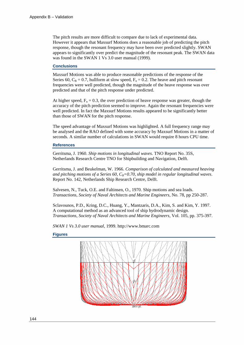
Appendix B – Validation
144
The pitch results are more difficult to compare due to lack of experimental data.
However it appears that Maxsurf Motions does a reasonable job of predicting the pitch
response, though the resonant frequency may have been over predicted slightly. SWAN
appears to significantly over predict the magnitude of the resonant peak. The SWAN data
was found in the SWAN 1 Vs 3.0 user manual (1999).
Conclusions
Maxsurf Motions was able to produce reasonable predictions of the response of the
Series 60, CB = 0.7, hullform at slow speed, Fn = 0.2. The heave and pitch resonant
frequencies were well predicted, though the magnitude of the heave response was over
predicted and that of the pitch response under predicted.
At higher speed, Fn = 0.3, the over prediction of heave response was greater, though the
accuracy of the pitch prediction seemed to improve. Again the resonant frequencies were
well predicted. In fact the Maxsurf Motions results appeared to be significantly better
than those of SWAN for the pitch response.
The speed advantage of Maxsurf Motions was highlighted. A full frequency range may
be analysed and the RAO defined with some accuracy by Maxsurf Motions in a matter of
seconds. A similar number of calculations in SWAN would require 8 hours CPU time.
References
Gerritsma, J. 1960. Ship motions in longitudinal waves. TNO Report No. 35S,
Netherlands Research Centre TNO for Shipbuilding and Navigation, Delft.
Gerritsma, J. and Beukelman, W. 1966. Comparison of calculated and measured heaving
and pitching motions of a Series 60, CB=0.70, ship model in regular longitudinal waves.
Report No. 142, Netherlands Ship Research Centre, Delft.
Salvesen, N., Tuck, O.E. and Faltinsen, O., 1970. Ship motions and sea loads.
Transactions, Society of Naval Architects and Marine Engineers, No. 78, pp 250-287.
Sclavounos, P.D., Kring, D.C., Huang, Y., Mantzaris, D.A., Kim, S. and Kim, Y. 1997.
A computational method as an advanced tool of ship hydrodynamic design.
Transactions, Society of Naval Architects and Marine Engineers, Vol. 105, pp. 375-397.
SWAN 1 Vs 3.0 user manual, 1999. http://www.bmarc.com
Figures
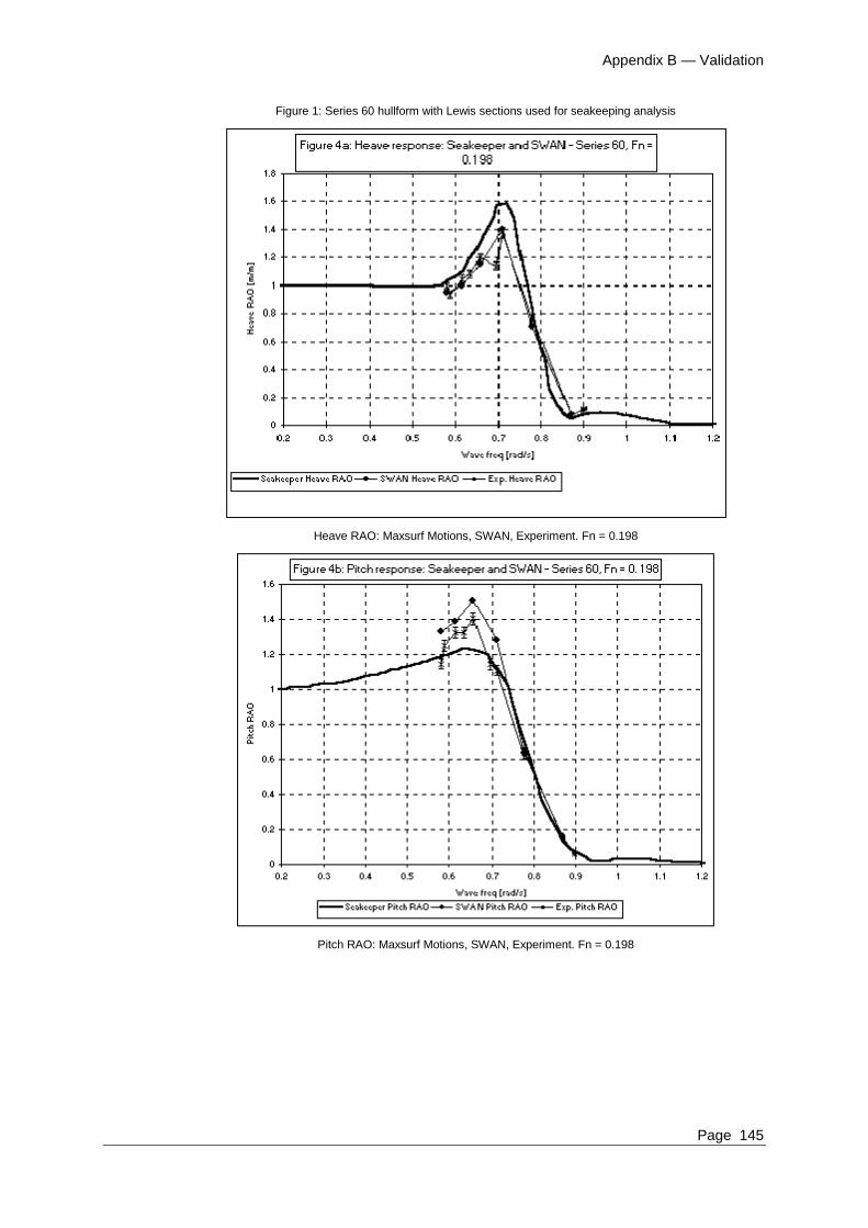
Appendix B — Validation
Page 145
Figure 1: Series 60 hullform with Lewis sections used for seakeeping analysis
Heave RAO: Maxsurf Motions, SWAN, Experiment. Fn = 0.198
Pitch RAO: Maxsurf Motions, SWAN, Experiment. Fn = 0.198

Appendix B – Validation
146
Heave RAO: Maxsurf Motions, SWAN, Experiment. Fn = 0.297
Pitch RAO: Maxsurf Motions, SWAN, Experiment. Fn = 0.297
Maxsurf Motions Validation 3 – SA van der Stel
The results from Maxsurf Motions for added resistance, heave and pitch have been
compared with results from tank tests and another strip theory program in head seas.
Hullform and test conditions
The hullform tested is that of the SA van der Stel, a fast freight vessel. The body plan is
shown below:

Appendix B — Validation
Page 147
SA van der Stel Body plan
The vessel has the following dimensions:
Full load
LengthPP Lpp 152.50m
Breadth B 22.80m
Amidships draught d 9.14m
Trim by sten trim 0.00m
Block coefficient Cb 0.563
Centre above base KG 9.14m
Radius gyration pitch kyy 0.22 % Lpp
Number of sections used for
seakeeping analysis
21
Number of conformal mapping
parameters per section
8
Water density 1000.00kg/m^3
Acceleration due to gravity g 9.80665m/s^2
The mapped sections (green) can be seen superimposed on the hull sections below:
Conformal mapping sections (green) used in Maxsurf Motions
The vessel was tested at four Froude numbers. No transom terms were used in the
Maxsurf Motions analysis.
Fn v m/s v kts
0.15 5.80 11.28
0.20 7.73 15.04
0.25 9.67 18.79
0.30 11.60 22.55

Appendix B – Validation
148
Results
The data were obtained from results published by Journee 2001. Results are given for
two sets of experimental results (circles) and two methods in another strip theory
implementation (grey lines). Maxsurf Motions v13 has three methods available for
estimating added resistance. One by Salvesen and two by Geritsma and Beukelman (they
offer two slightly different formulations). A third method by Havelock is being
implemented and is included for comparison.
Fn = 0.15
Fn = 0.15 Head seas
0
2.5
5
7.5
10
12.5
0.5 0.75 1 1.25 1.5
sqrt(Lpp/lambda)
Ra
w/(
rho
g z
eta
^2
B^
2/L
pp
)
Salvesen
Gerritsma and Beukelman I
Gerritsma and Beukelman II
Havelock
Exp. (G&B)
Exp.
Seaway (G&B)
Seaway Boese
Added resistance for SA van der Stel; Fn = 0.15; Head seas
Fn = 0.15 Head seas
0
0.5
1
1.5
2
0.5 0.75 1 1.25 1.5
sqrt(Lpp/lambda)
He
av
e R
AO
Heave RAO
Exp. (G&B)
Exp.
Seaway
Heave response for SA van der Stel; Fn = 0.15; Head seas
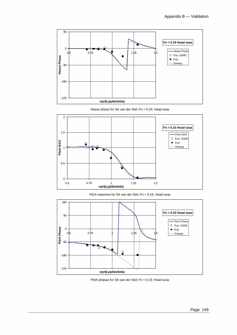
Appendix B — Validation
Page 149
Fn = 0.15 Head seas
-270
-180
-90
0
90
0.5 0.75 1 1.25 1.5
sqrt(Lpp/lambda)
He
av
e P
ha
se
Heave Phase
Exp. (G&B)
Exp.
Seaway
Heave phase for SA van der Stel; Fn = 0.15; Head seas
Fn = 0.15 Head seas
0
0.5
1
1.5
2
0.5 0.75 1 1.25 1.5
sqrt(Lpp/lambda)
Pit
ch
RA
O
Pitch RAO
Exp. (G&B)
Exp.
Seaway
Pitch response for SA van der Stel; Fn = 0.15; Head seas
Fn = 0.15 Head seas
-270
-180
-90
0
90
180
0.5 0.75 1 1.25 1.5
sqrt(Lpp/lambda)
Pit
ch
Ph
as
e
Pitch Phase
Exp. (G&B)
Exp.
Seaway
Pitch phasee for SA van der Stel; Fn = 0.15; Head seas

Appendix B – Validation
150
Fn = 0.20
Fn = 0.20 Head seas
0
2.5
5
7.5
10
12.5
0.5 0.75 1 1.25 1.5
sqrt(Lpp/lambda)
Ra
w/(
rho
g z
eta
^2
B^
2/L
pp
)
Salvesen
Gerritsma and Beukelman I
Gerritsma and Beukelman II
Havelock
Exp. (G&B)
Exp.
Seaway (G&B)
Seaway Boese
Added resistance for SA van der Stel; Fn = 0.20; Head seas
Fn = 0.25
Fn = 0.25 Head seas
0
2.5
5
7.5
10
12.5
15
0.5 0.75 1 1.25 1.5
sqrt(Lpp/lambda)
Ra
w/(
rho
g z
eta
^2
B^
2/L
pp
)
Salvesen
Gerritsma and Beukelman I
Gerritsma and Beukelman II
Havelock
Exp. (G&B)
Exp.
Seaway (G&B)
Seaway Boese
Added resistance for SA van der Stel; Fn = 0.25; Head seas

Appendix B — Validation
Page 151
Fn = 0.30
Fn = 0.30 Head seas
0
2.5
5
7.5
10
12.5
15
0.5 0.75 1 1.25 1.5
sqrt(Lpp/lambda)
Ra
w/(
rho
g z
eta
^2
B^
2/L
pp
)
Salvesen
Gerritsma and Beukelman I
Gerritsma and Beukelman II
Havelock
Exp. (G&B)
Exp.
Seaway (G&B)
Seaway Boese
Added resistance for SA van der Stel; Fn = 0.30; Head seas
Fn = 0.30 Head seas
0
0.5
1
1.5
2
0.5 0.75 1 1.25 1.5
sqrt(Lpp/lambda)
He
av
e R
AO
Heave RAO
Exp. (G&B)
Exp.
Seaway
Heave response for SA van der Stel; Fn = 0.30; Head seas
Fn = 0.30 Head seas
-270
-180
-90
0
90
180
0.5 0.75 1 1.25 1.5
sqrt(Lpp/lambda)
He
av
e P
ha
se
Heave Phase
Exp. (G&B)
Exp.
Seaway
Heave phase for SA van der Stel; Fn = 0.30; Head seas

Appendix B – Validation
152
Fn = 0.30 Head seas
0
0.5
1
1.5
2
0.5 0.75 1 1.25 1.5
sqrt(Lpp/lambda)
Pit
ch
RA
O
Pitch RAO
Exp. (G&B)
Exp.
Seaway
Pitch response for SA van der Stel; Fn = 0.30; Head seas
Fn = 0.30 Head seas
-270
-180
-90
0
90
180
0.5 0.75 1 1.25 1.5
sqrt(Lpp/lambda)
Pit
ch
Ph
as
e
Pitch Phase
Exp. (G&B)
Exp.
Seaway
Pitch phasee for SA van der Stel; Fn = 0.30; Head seas
Conclusions
All results show the characteristic peak with frequency for the added resistance response.
The Gerritsma and Beukelman methods show some differences but reproduce the
experimental data reasonably well – as does the Havelock method. The Salvesen method
does not reproduce the experimental results with as much accuracy as the other methods
for this hullform.
It should be noted that there is considerable scatter in the experimental results and that
the peaks of the response are not well captured by the experiments in all cases, due to
insufficient data. It has been the author’s experience that it is extremely difficult to
measure added resistance with high accuracy in the towing tank. To the author’s
knowledge no accurate full scale added resistance measurements have been reported in
the scientific literature for investigation of scaling effects etc. For these reasons it is felt
that the added resistance methods available in Maxsurf Motions produce results of
sufficient quality for comparative hullform analysis in the early design stage.
Bibliography
J.M.J. Journée 2001: Veri…cation and Validation of Ship Motions Program SEAWAY,
Delft University of Technology Shiphydromechanics Laboratory Report1213a

Appendix B — Validation
Page 153
Jasna Prpić-Oršić, Radoslav Nabergoj and Giorgio Trincas 2008: The methods of added
resistance estimation for ships in a seaway, 18th Symposium on Theory and Practice of
Shipbuilding
F. Pe´rez Arribas 2007: Some methods to obtain the added resistance of a ship advancing
in waves, Ocean Engineering 34 946–955

Appendix B – Validation
154
Appendix C Panel Method Formulation
LINEAR POTENTIAL THEORY
Coordinates and Boundary Value Problem
For the mathematical descriptions of fluid and body motions, a body fixed coordinates
system is adopted. By introducing the centre of rotation, the body motions are able to be
described with respect to a translated coordinates system.
Body Fixed Coordinates and Centre of Rotation
The wave height and steepness are also assumed to be small so that the linear wave
theory may be used. The fluid is assumed to be incompressible and inviscid, and the flow
be irrotational. Thus the flow field can be described by the gradient of a velocity
potential, which is governed by the Laplace equation and at the same time it should
satisfy the proper boundary conditions. For harmonic motions, the velocity potential may
be written as follows:
Within the framework of linear theory, the velocity potential is subdivided into the
incident potential , the diffraction potential , and the radiation potential .
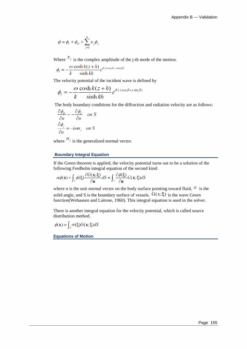
Appendix B — Validation
Page 155
Where is the complex amplitude of the j-th mode of the motion.
The velocity potential of the incident wave is defined by
The body boundary conditions for the diffraction and radiation velocity are as follows:
where is the generalized normal vector.
Boundary Integral Equation
If the Green theorem is applied, the velocity potential turns out to be a solution of the
following Fredholm integral equation of the second kind:
where n is the unit normal vector on the body surface pointing toward fluid, is the
solid angle, and S is the boundary surface of vessels. is the wave Green
function(Wehausen and Laitone, 1960). This integral equation is used in the solver.
There is another integral equation for the velocity potential, which is called source
distribution method.
Equations of Motion

Appendix B – Validation
156
Here we assume that the body is rigid and in a state of stable equilibrium when in calm
water. By considering the hydrodynamic forces acting on the body, the equations of
motion are obtained in the form
where is the viscous damping matrix. and are hydrostatic restoring and
external mooring stiffness matrix, respectively.
Mean Drift Forces and Moments
The mean drift forces and moments are evaluated based on direct pressure integration
method. Pinkster and Oortmerssen (1997) derived second order drift force and moments
acting on the floating body as follows:
where is the relative wave elevation along the waterline, and the oscillatory
first order angular motion vector. Fifth terms above equations are the contribution of the
second order potential to the drift forces and moments. They will not contribute to the
mean drift forces and moments.

Appendix B — Validation
Page 157
Appendix D Panel Method Validation
Validation with experiment
“Catamaran Motions in Beam and Oblique Seas” - Thomas, Doctors, Couser and
Hackett - Ninth International Conference on Fast Sea Transportation, FAST2007,
Shanghai, China, September 2007.
s/l = demihull spacing/length overall
Demi-hull body plan
Results:
All experiments and analysis conducted at zero fwd speed.

Appendix B – Validation
158
Heading = 90 deg, s/l=0.4
Heading = 90 deg, s/l=0.2

Appendix B — Validation
Page 159
Heading = 90 deg, s/l=0.4
Heading = 90 deg, s/l=0.2

Appendix B – Validation
160
Heading = 90 deg, s/l=0.4
Heading = 90 deg, s/l=0.2

Appendix B — Validation
Page 161
Verification against WAMIT
WAMIT (WaveAnalysisMIT) is a commercially available software package for
computing wave loads and motions of offshore structures in waves. WAMIT solves the
velocity potential by means of boundary integral equation method (panel method). It
first version was launched in 1987. Following are results of motions analysis conducted
on a box shaped barge using the Maxsurf Motions panel method compared with the
WAMIT panel method.
Analysis parameters:
Geometry : Length = 200m, Beam = 40m, Draft = 28m.
CoG = Centre of Waterplane
Pitch gyradius = 60m
Yaw gyradius = 60m
Roll gyradius = 20m
Characteristic length (L) = 61m.
Characteristic wave amplitude (A) = 1m
Zero Fwd Speed.
Heading = 180 deg (head seas).
Motions

Appendix B – Validation
162
Wave forces
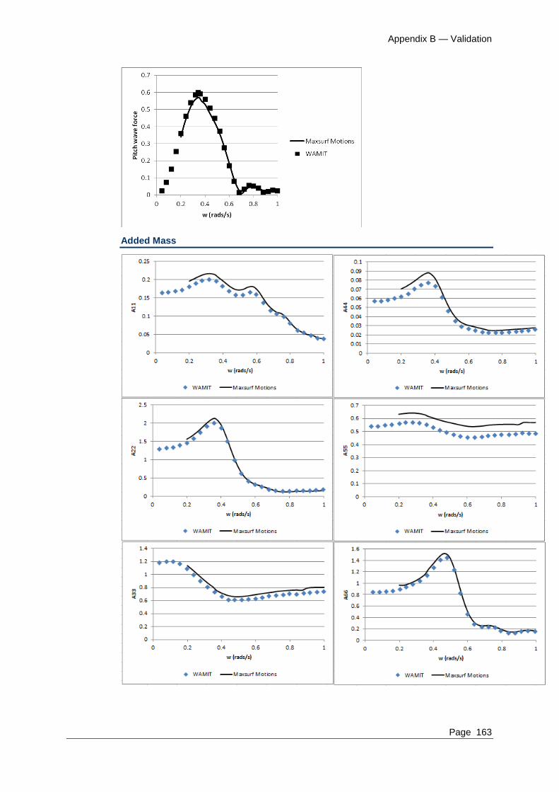
Appendix B — Validation
Page 163
Added Mass
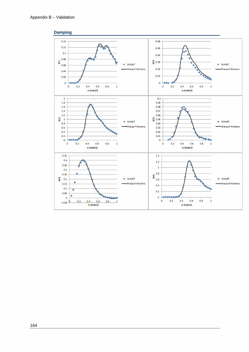
Appendix B – Validation
164
Damping

Appendix B — Validation
Page 165
Drift Forces

Appendix B – Validation
166
Verification against AQWA
AQWA is a commercially available software package for computing wave loads and
motions of offshore structures in waves. Seakeeping tests to determine the motion
transfer functions for the Incat 112 were conducted in the Australian Maritime College's
model test basin.

Appendix B — Validation
Page 167

Appendix B – Validation
168

Appendix B — Validation
Page 169

Index
170
Index
A
About Seakeeper ........................................... 64
Absolute Motion ........................................... 23
Absolute Vessel Motions .............................. 77
Added Mass .................................................. 36
Added Mass and Damping of 2D Ship
Sections ................................................... 100
Added Mass at Infinite Frequency .............. 103
Added Resistance .......................................... 28
Added Resistance of a Vessel in a Seaway ... 98
Additional Hull Parameters ........................... 19
Analysis Menu .............................................. 60
Analysis Method ........................................... 61
Analysis Toolbar ........................................... 56
Animate ......................................................... 62
Animation ..................................................... 47
Arbitrary Wave Heading ............................... 95
Arrange Icons ................................................ 63
Assumptions .................................................... 4
Asymmetrical sections .................................. 18
Automation Reference .................................. 63
Average 1/nth highest amplitudes .................. 78
B
Bandwidth ..................................................... 68
Bibliography ................................................. 88
Bretschneider .......................................... 27, 69
BS 6841
1987 .................................................... 33, 82
C
Calculating Vessel Motions ...................... 9, 76
Calculation and integration of pressure
functions around contour ........................ 102
Calculation of Mapped Sections ................... 29
Cascade ......................................................... 63
Catamaran, Roll ............................................ 20
Catamarans .................................................... 20
CG RAOs ...................................................... 34
Characterisation .............................................. 6
Characterising Vessel Response ............... 8, 73
Check for Updates ......................................... 64
Checking the Solution ................................. 103
Close Design ................................................. 57
Colour ........................................................... 60
Completing the Analysis ............................... 27
Computational Methods ................................ 10
Conformal Mapping ...................................... 10
Contour Toolbar ............................................ 56
Coordinate System .......................................... 5
Copy.............................................................. 59
D
Damping ........................................... 22, 36, 61
Damping coefficient ..................................... 22
Damping Factors ..................................... 22, 61
Damping parameter ...................................... 22
Data Menu .................................................... 62
demihull centreline spacing .......................... 20
Derivative of Conformal Mapping ............. 106
Diffraction Force .......................................... 96
Display Menu ............................................... 61
DNV.............................................................. 27
DNV Spectrum ............................................. 70
Draft .............................................................. 18
DWL ............................................................. 18
E
Edit Menu ..................................................... 58
Encounter Frequency .................................... 72
Encounter Period .......................................... 72
Encounter Spectrum.................................. 8, 73
Environment ........................................... 25, 61
Environmental Parameters ............................ 25
Evaluation of hydrodynamic coefficients ... 103
Exit................................................................ 58
F
File Menu ...................................................... 57
File Toolbar .................................................. 55
Font ............................................................... 60
Frame of Reference....................................... 63
Frame Of Reference ...................................... 18
Frank Close Fit ............................................. 10
Frequency Range .................................... 27, 61
Froude Number ............................................. 26
Froude-Krilov Force ..................................... 97
G
Getting Started .............................................. 13
Global Added Mass and Damping (Strip
Theory) ..................................................... 93
Global Hydrodynamic Coefficients .............. 35
Glossary ........................................................ 86
Graph ............................................................ 63
Graph Options ......................................... 38, 62
Graph Window ............................................. 54
Graph window Toolbar ................................. 56
Graphing the Results..................................... 38
Grid ............................................................... 61

Index
Page 171
H
Harmonic Response of Damped, Spring, Mass
system ......................................................... 8
Harmonic Response of Damped, Spring, Mass
System ....................................................... 74
Head Seas Approximation ............................ 97
Heading ......................................................... 48
Headings ....................................................... 25
Heave and Pitch Motion of a Vessel in a
Seaway ...................................................... 92
Help Menu .................................................... 63
Home View ................................................... 59
Hydrodynamic Component ......................... 109
Hydrostatic (Restoring) Component ........... 107
I
Idealised Spectra ....................................... 7, 69
Important notes ........................................... 103
Inertial Component ..................................... 107
ISO 2631/3 1985 ........................................... 82
ISO 2631/3 1985 ........................................... 33
ITTC ........................................................ 27, 69
J
Joint Probability ............................................ 81
JONSWAP .............................................. 27, 70
L
Least squares solution to over-defined set of
linear equations ....................................... 101
Lewis Sections ........................................ 16, 30
Limitations and Guidelines ........................... 50
Long-Term Statistics ..................................... 80
M
m0 .................................................................. 31
Mass Distribution .................................... 21, 61
Measure Hull ............................... 16, 29, 60, 61
Menus ............................................................ 56
MII ................................................................ 23
Most probable largest value .......................... 79
Most probable value
Modal value .............................................. 79
Motion periods .............................................. 79
MSI ............................................. 32, 33, 82, 83
Exposure time ........................................... 24
Multipole expansion coefficients ................ 100
N
Nomenclature ................................................ 86
Non-Dimensional Added Mass ................... 104
Non-Dimensional Damping Coefficient ..... 103
Non-Dimensional Frequency ...................... 104
O
Occurrence per hour ..................................... 80
Online Support .............................................. 63
Open Design ................................................. 57
Open Seakeeper Data .................................... 57
P
Page Setup .................................................... 58
Pan ................................................................ 59
Paste .............................................................. 59
Pierson Moskowitz ................................. 27, 71
Pitch Gyradius ........................................ 21, 61
Polar Plots ..................................................... 40
Polar Window ............................................... 55
Preferences .................................................... 13
Print .............................................................. 58
Probability Measures .................................... 80
Probability of Exceeding a Critical Value .... 80
R
Relative Motion ............................................ 23
Remote Location ........................................... 23
Remote location display ............................... 24
Remote Location Spectra .............................. 34
Remote Location, Adding ............................. 25
Remote Location, Deleting ........................... 25
Remote Location, Results ............................. 25
Render ........................................................... 62
Render ........................................................... 41
Representation of Ship-Like Sections by
Conformal Mapping................................ 104
Response Amplitude Operator .................. 8, 76
Results Toolbar ............................................. 56
Results Window ............................................ 53
Results, saving .............................................. 49
RMS .............................................................. 31
Roll Damping ............................................... 61
Roll decay simulation ................................... 43
Roll decay test .............................................. 22
Roll Gyradius .......................................... 21, 61
Rotate ............................................................ 59
S
Salvesen et al. (1970) Approximation .......... 98
Save … Results As ....................................... 58
Save CG RAOs Results As ........................... 58
Save CG spectra Results As ......................... 58
Save Global hydrodynamic coeffs. Results As
.................................................................. 58
Save MSI Results As ................................... 58
Save Remote location spectra Results As ..... 58
Save Seakeeper Data..................................... 57
Save Seakeeper Data As ............................... 57

Index
172
Save Sectional hydrodynamic coeffs. Results
As .............................................................. 58
Save Summary Results As ........................... 58
Sea State Codes ............................................... 6
Seakeeping Fundamentals ............................... 4
Section Data ............................................ 39, 62
Sectional Hydrodynamic Coefficients .......... 36
Set Home View ............................................. 59
Shear Force and Bending Moment due to Ship
Motion in a Seaway ................................ 106
Shift Key ....................................................... 13
Ship Sections, 2D ........................................ 100
Short-Term statistics ..................................... 78
Shrink ............................................................ 59
Significant Amplitude ................................... 31
Significant Wave Height ............................... 68
Solution of Coupled Heave and Pitch Motions
.................................................................. 93
Solve Seakeeping Analysis ..................... 30, 61
Spectra .......................................................... 25
Spectral Characteristics ................................. 67
Speed ............................................................. 48
Speed Loss .................................................... 84
Speeds ........................................................... 25
Statistical Measures .................................. 9, 78
Stiffness ........................................................ 36
Strip Theory .................................................. 10
Strip theory formulation ................................ 91
Subjective Magnitude ............................. 32, 81
Subjective Magnitude scale .......................... 33
Summary Table ............................................. 31
Surface, irregular waves ................................ 45
Surface, regular waves .................................. 44
Surface, Roll decay simulation ..................... 43
Surface, static (flat) ....................................... 42
Surface, wavy ................................................ 46
T
Table of Contents .......................................... 63
Tile Horizontal .............................................. 63
Tile Vertical .................................................. 63
Time simulation ............................................ 47
Toolbars ........................................................ 55
Transfer Function............................................ 8
Transom Terms ............................................. 28
Trim Surfaces ............................................... 16
U
Underlying Assumptions .............................. 50
Units.............................................................. 62
V
Validation ................................................... 115
Velocity and Acceleration Spectra ............... 79
Vertical Centre of Gravity (VCG) ................ 22
Vessel Speed ................................................. 52
Vessel Type .................................................. 61
Vessel Type .................................................. 20
View Menu ................................................... 59
View Toolbar ................................................ 55
Viewing the Results ...................................... 31
Visualisation ................................................. 11
W
Wave Attenuation (Smith Effect) ................. 98
Wave Energy ................................................ 67
Wave Excitation............................................ 36
Wave Excitation Component ...................... 108
Wave Excitation Force and Moment ............ 95
Wave Force ................................................... 29
Wave Heading .............................................. 52
Wave Spectra ............................................ 6, 67
Wave spectra input ....................................... 26
Wave Spectra Representation ................... 7, 67
Wave Spectrum ............................................. 48
What the Vessel Sees .................................... 72
Window Menu .............................................. 63
Window Toolbar ........................................... 56
Windows ....................................................... 53
Windows Registry ........................................ 13
Z
Zoom ............................................................. 59