motion planning, part iv graph search part ii
TRANSCRIPT

Motion Planning, Part IV
Graph Search Part II
Howie Choset

Map-Based Approaches:
Roadmap Theory • Properties of a roadmap:
– Accessibility: there exists a collision-free
path from the start to the road map
– Departability: there exists a collision-free
path from the roadmap to the goal.
– Connectivity: there exists a collision-free
path from the start to the goal (on the
roadmap).
a roadmap exists a path exists
Examples of Roadmaps – Generalized Voronoi Graph (GVG)
– Visibility Graph

The Visibility Graph in Action (Part 1)
• First, draw lines of sight from the start and goal to all
“visible” vertices and corners of the world.
start
goal

The Visibility Graph in Action (Part 2)
• Second, draw lines of sight from every vertex of every obstacle
like before. Remember lines along edges are also lines of sight.
start
goal

The Visibility Graph in Action (Part 3)
• Second, draw lines of sight from every vertex of every obstacle
like before. Remember lines along edges are also lines of sight.
start
goal

The Visibility Graph in Action (Part 4)
• Second, draw lines of sight from every vertex of every obstacle
like before. Remember lines along edges are also lines of sight.
start
goal

The Visibility Graph (Done)
• Repeat until you’re done.
start
goal

Graph Search Howie Choset
16-311

9
Informed Search: A*
Notation
• n → node/state
• c(n1,n2) → the length of an edge connecting
between n1 and n2
• b(n1) = n2 → backpointer of a node n1 to a
node n2.

10
Informed Search: A*
• Evaluation function, f(n) = g(n) + h(n)
• Operating cost function, g(n)
– Actual operating cost having been already traversed
• Heuristic function, h(n)
– Information used to find the promising node to traverse
– Admissible → never overestimate the actual path cost
Cost on a grid

11
Example (1/5)
h(x)
c(x)
Legend
Priority = g(x) + h(x)
g(x) = sum of all previous arc costs, c(x),
from start to x
Example: c(H) = 2 GOAL
3 3 3
3
3
3 3
1
1 2 2
3
3
3
2
2
0 Start
2
2 4 1
1
1 1
1
1 1
1 1
A
B
C D
E F
G H I
J K
L
Note:

12
Example (2/5)
B(3)
A(4)
C(4)
H(3)
A(4)
C(4)
I(5)
G(7)
First expand the start node
If goal not found,
expand the first node
in the priority queue
(in this case, B)
Insert the newly expanded
nodes into the priority queue
and continue until the goal is
found, or the priority queue is
empty (in which case no path
exists) Note: for each expanded node,
you also need a pointer to its respective
parent. For example, nodes A, B and C
point to Start
GOAL
3 3 3
3
3
3 3
1
1 2 2
3
3
3
2
2
0 Start
2
2 4 1
1
1 1
1
1 1
1 1
A
B
C D
E F
G H I
J K
L

13
Example (3/5) B(3)
A(4)
C(4)
H(3)
A(4)
C(4)
I(5)
G(7)
No expansion
E(3)
C(4)
D(5)
I(5)
F(7)
G(7)
GOAL(5)
We’ve found a path to the goal:
Start => A => E => Goal (from the pointers)
Are we done? GOAL
3 3 3
3
3
3 3
1
1 2 2
3
3
3
2
2
0 Start
2
2 4 1
1
1 1
1
1 1
1 1
A
B
C D
E F
G H I
J K
L

14
Example (4/5) B(3)
A(4)
C(4)
H(3)
A(4)
C(4)
I(5)
G(7)
No expansion
E(3)
C(4)
D(5)
I(5)
F(7)
G(7)
GOAL(5)
There might be a shorter path, but assuming
non-negative arc costs, nodes with a lower priority
than the goal cannot yield a better path.
In this example, nodes with a priority greater than or
equal to 5 can be pruned.
Why don’t we expand nodes with an equivalent priority?
(why not expand nodes D and I?)
GOAL
3 3 3
3
3
3 3
1
1 2 2
3
3
3
2
2
0 Start
2
2 4 1
1
1 1
1
1 1
1 1
A
B
C D
E F
G H I
J K
L

15
Example (5/5) B(3)
A(4)
C(4)
H(3)
A(4)
C(4)
I(5)
G(7)
No expansion
E(3)
C(4)
D(5)
I(5)
F(7)
G(7)
GOAL(5)
We can continue to throw away nodes with
priority levels lower than the lowest goal found.
As we can see from this example, there was a
shorter path through node K. To find the path, simply
follow the back pointers.
Therefore the path would be:
Start => C => K => Goal
K(4)
L(5)
J(5)
GOAL(4)
If the priority queue still wasn’t empty, we would
continue expanding while throwing away nodes
with priority lower than 4.
(remember, lower numbers = higher priority)
GOAL
3 3 3
3
3
3 3
1
1 2 2
3
3
3
2
2
0 Start
2
2 4 1
1
1 1
1
1 1
1 1
A
B
C D
E F
G H I
J K
L

16
Monotonic • never overestimates the cost of getting from a node
to its neighbor.
• for all paths x,y where y is a successor of x, i.e.,
• h(A) = 3 g(A) = 1 h(E) = 1 g(E) = 2
h(y) g(x) - g(y) h(x)
2 11-2 h(E)g(A)-g(E) 3h(A)

17
Non-opportunistic 1. Put S on priority Q and expand it
2. Expand A because its priority value is 7
3. The goal is reached with priority value 8
4. This is less than B’s priority value which is 13

Roadmap: GVG
• A GVG is
formed by paths
equidistant from
the two closest
objects
• Remember
“spokes”, start
and goal
• This generates a very safe roadmap which avoids obstacles as
much as possible

Distance to Obstacle(s)
)(min)( qdqD i

Two-Equidistant • Two-equidistant surface
}0)()(:{ free xdxdQxS jiij
iQO
jQO

More Rigorous Definition
Going through obstacles
Two-equidistant face
},),()()(:{ jihxdxdxdSSxF hjiijij
iQO
jQO )()()( xdxdxd jik ij SS
kQO

General Voronoi Diagram
1
1 1
GVD
n
i
n
ij
ijF

What about concave obstacles?
vs

What about concave obstacles?
vs
id
jd
id
jd

What about concave obstacles?
vs
id
jd
id
jd
id
jd
jd
id

Two-Equidistant • Two-equidistant surface
Two-equidistant surjective surface
Two-equidistant Face
}0)()(:{ free xdxdQxS jiij
jC
iC
ij S
id
jd
)}()(:{ xdxdSxSS jiijij
}),()(:{ ihxdxdSSxF hiijij
1
1 1
GVD
n
i
n
ij
ijF

Voronoi Diagram: Metrics

Voronoi Diagram (L2)
Note the
curved
edges

Voronoi Diagram (L1)
Note the
lack of
curved
edges

Exact Cell vs. Approximate Cell
• Cell: simple region

Adjacency Graph – Node correspond to a cell
– Edge connects nodes of adjacent cells • Two cells are adjacent if they share a common boundary
c11
c1
c2
c4
c3
c6
c5 c8
c7
c
10
c9
c12
c13
c14
c15
c1 c10
c2
c3
c4 c5
c6
c7
c8
c9
c11
c12
c13
c14
c15

Set Notation

Examples

Definition

Cell Decompositions: Trapezoidal Decomposition
• A way to divide the world into smaller regions
• Assume a polygonal world

Cell Decompositions: Trapezoidal Decomposition
• Simply draw a vertical line from each vertex until you hit an obstacle. This
reduces the world to a union of trapezoid-shaped cells

Applications: Coverage
• By reducing the world to cells, we’ve essentially abstracted the world to a
graph.

Find a path
• By reducing the world to cells, we’ve essentially abstracted the world to a
graph.

Find a path
• With an adjacency graph, a path from start to goal can be found by simple
traversal
start goal

Find a path
• With an adjacency graph, a path from start to goal can be found by simple
traversal
start goal

Find a path
• With an adjacency graph, a path from start to goal can be found by simple
traversal
start goal

Find a path
• With an adjacency graph, a path from start to goal can be found by simple
traversal
start goal

Find a path
• With an adjacency graph, a path from start to goal can be found by simple
traversal
start goal

Find a path
• With an adjacency graph, a path from start to goal can be found by simple
traversal
start goal

Find a path
• With an adjacency graph, a path from start to goal can be found by simple
traversal
start goal

Find a path
• With an adjacency graph, a path from start to goal can be found by simple
traversal
start goal

Find a path
• With an adjacency graph, a path from start to goal can be found by simple
traversal
start goal

Find a path
• With an adjacency graph, a path from start to goal can be found by simple
traversal
start goal

Find a path
• With an adjacency graph, a path from start to goal can be found by simple
traversal
start goal

Connect Midpoints of Traps

Applications: Coverage
• First, a distinction between sensor and detector must be made
• Sensor: Senses obstacles
• Detector: What actually does the coverage
• We’ll be observing the simple case of having an omniscient sensor and having the detector’s footprint equal to the robot’s footprint

Howie Choset
Robotics Institute
(snake robots)

Cell Decompositions: Trapezoidal Decomposition
• How is this useful? Well, trapezoids can easily be covered with simple back-and-forth sweeping motions. If we cover all the trapezoids, we can effectively cover the entire “reachable” world.
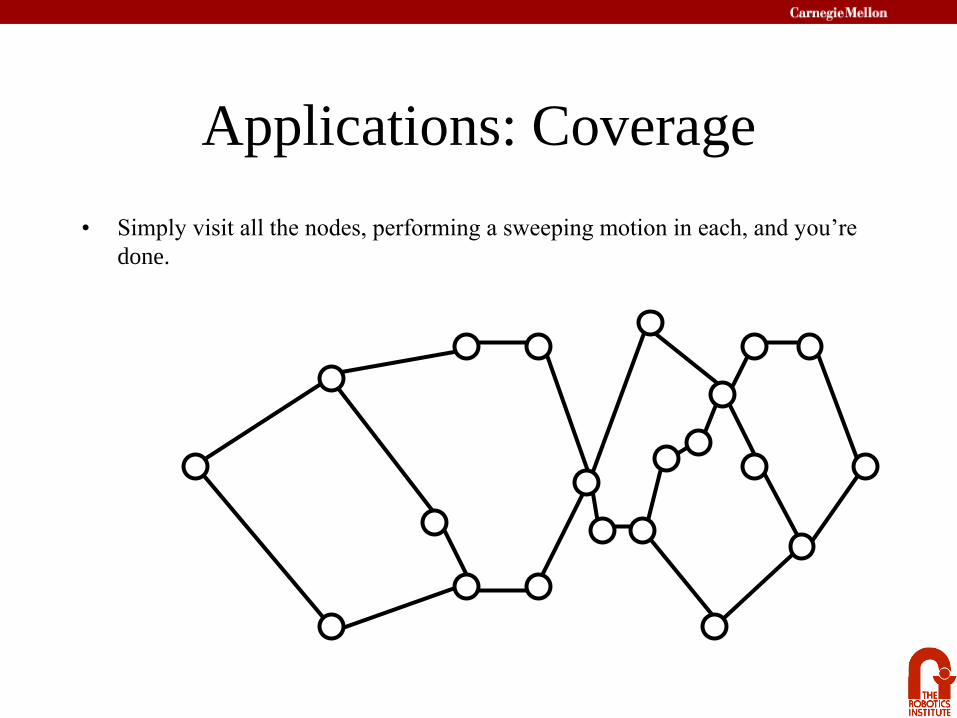
Applications: Coverage
• Simply visit all the nodes, performing a sweeping motion in each, and you’re
done.

•Slice is a level set
•Slice function: h(x,y)= x, slice={(x,y)|h(x,y)=}
• At a critical point x of where M = {x|m(x)=0} )()(,| xmxhh M
h
m
Cell Decomp. in Terms of Critical Points

1-connected
h(x,y) = a1

2-connected
h(x,y) = a2

1-connected
h(x,y) = a3

2-connected
h(x,y) = a4

• Connectivity of the slice in the free space
changes at the critical points (Morse theory)
a1 a2 a3 a4

• Each cell can be covered by back and
forth motions

Cell-Decomposition Approach
• Define Decomposition
– Completeness
• Sensor-based Construction
• Define Other Decompositions
– Other patterns
– Extended detector

Provably completeness = guaranteed completeness

25m x 30m Successful Experiment: Stopped because of robot battery limitations
Simultaneous Coverage* and
Localization
*mapping too

Path Planning Where to cover and map
Position Planning How to collaboratively move and
maintain low position error (w/o
GPS)
Local Planning Obstacle detection/avoidance
Terrain features to inform Path
Planner
Operational Hierarchy
Calibrate robots’ initial location and go

Probabilistic Coverage

Surface Deposition
• Process Variables
– Uniformity
– Waste
– Positioning
• Cycle-time
– Time-to-completion
– Programming time

Conclusion: Complete Overview
• The Basics – Motion Planning Statement
– The World and Robot
– Configuration Space
– Metrics
• Path Planning Algorithms – Start-Goal Methods
• Lumelsky Bug Algorithms
• Potential Charge Functions
• The Wavefront Planner
– Map-Based Approaches
• Generalized Voronoi Graphs
• Visibility Graphs
– Cellular Decompositions => Coverage
• Done with Motion Planning!