Motion Planning for Paramagnetic MicroparticlesUnder Motion and Sensing Uncertainty

Wen Sun1, Islam S. M. Khalil2, Sarthak Misra3, and Ron Alterovitz1

Abstract— Paramagnetic microparticles moving through flu-ids have the potential to be used in many applications, in-cluding microassembly, micromanipulation, and highly local-ized delivery of therapeutic agents inside the human body.Paramagnetic microparticles with diameters of approximately100 µm can be wirelessly controlled by externally applyingmagnetic field gradients using electromagnets. In this paper, weintroduce a motion planner to guide a spherical paramagneticmicroparticle to a target while avoiding obstacles. The motionplanner explicitly considers uncertainty in the microparticle’smotion and maximizes the probability that the microparticleavoids obstacle collisions and reaches the target. To enableeffective consideration of uncertainty, we use an ExpectationMaximization (EM) algorithm to learn a stochastic model ofthe uncertainty in microparticle motion and state sensing fromexperiments conducted in a 3D 8-electromagnet microparticletestbed. We apply the motion planner in a simulated 3Denvironment with static obstacles and demonstrate that thecomputed plans are more likely to result in task success thanplans based on traditional metrics such as shortest path ormaximum clearance.

I. INTRODUCTION

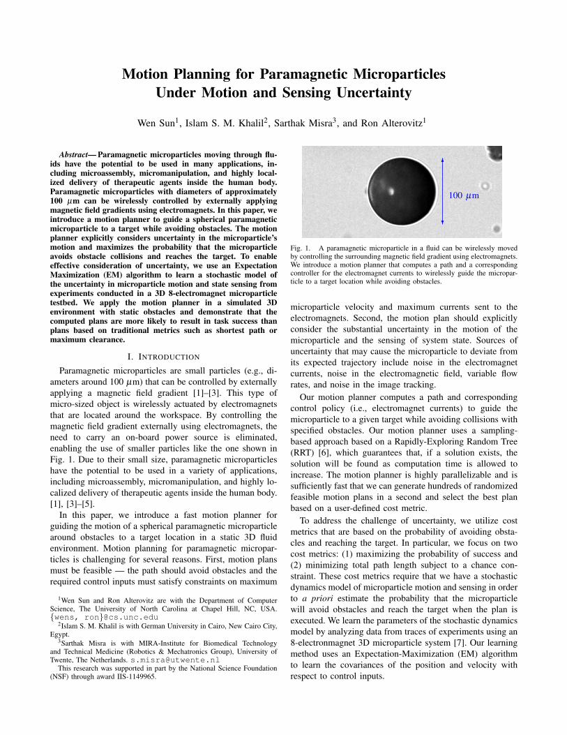
Paramagnetic microparticles are small particles (e.g., di-ameters around 100 µm) that can be controlled by externallyapplying a magnetic field gradient [1]–[3]. This type ofmicro-sized object is wirelessly actuated by electromagnetsthat are located around the workspace. By controlling themagnetic field gradient externally using electromagnets, theneed to carry an on-board power source is eliminated,enabling the use of smaller particles like the one shown inFig. 1. Due to their small size, paramagnetic microparticleshave the potential to be used in a variety of applications,including microassembly, micromanipulation, and highly lo-calized delivery of therapeutic agents inside the human body.[1], [3]–[5].

In this paper, we introduce a fast motion planner forguiding the motion of a spherical paramagnetic microparticlearound obstacles to a target location in a static 3D fluidenvironment. Motion planning for paramagnetic micropar-ticles is challenging for several reasons. First, motion plansmust be feasible — the path should avoid obstacles and therequired control inputs must satisfy constraints on maximum

1Wen Sun and Ron Alterovitz are with the Department of ComputerScience, The University of North Carolina at Chapel Hill, NC, USA.{wens, ron}@cs.unc.edu

2Islam S. M. Khalil is with German University in Cairo, New Cairo City,Egypt.

3Sarthak Misra is with MIRA-Institute for Biomedical Technologyand Technical Medicine (Robotics & Mechatronics Group), University ofTwente, The Netherlands. s.misra@utwente.nl

This research was supported in part by the National Science Foundation(NSF) through award IIS-1149965.

100 µm

6

?

Fig. 1. A paramagnetic microparticle in a fluid can be wirelessly movedby controlling the surrounding magnetic field gradient using electromagnets.We introduce a motion planner that computes a path and a correspondingcontroller for the electromagnet currents to wirelessly guide the micropar-ticle to a target location while avoiding obstacles.

microparticle velocity and maximum currents sent to theelectromagnets. Second, the motion plan should explicitlyconsider the substantial uncertainty in the motion of themicroparticle and the sensing of system state. Sources ofuncertainty that may cause the microparticle to deviate fromits expected trajectory include noise in the electromagnetcurrents, noise in the electromagnetic field, variable flowrates, and noise in the image tracking.

Our motion planner computes a path and correspondingcontrol policy (i.e., electromagnet currents) to guide themicroparticle to a given target while avoiding collisions withspecified obstacles. Our motion planner uses a sampling-based approach based on a Rapidly-Exploring Random Tree(RRT) [6], which guarantees that, if a solution exists, thesolution will be found as computation time is allowed toincrease. The motion planner is highly parallelizable and issufficiently fast that we can generate hundreds of randomizedfeasible motion plans in a second and select the best planbased on a user-defined cost metric.

To address the challenge of uncertainty, we utilize costmetrics that are based on the probability of avoiding obsta-cles and reaching the target. In particular, we focus on twocost metrics: (1) maximizing the probability of success and(2) minimizing total path length subject to a chance con-straint. These cost metrics require that we have a stochasticdynamics model of microparticle motion and sensing in orderto a priori estimate the probability that the microparticlewill avoid obstacles and reach the target when the plan isexecuted. We learn the parameters of the stochastic dynamicsmodel by analyzing data from traces of experiments using an8-electronmagnet 3D microparticle system [7]. Our learningmethod uses an Expectation-Maximization (EM) algorithmto learn the covariances of the position and velocity withrespect to control inputs.

Our objective of explicitly considering uncertainty duringmotion planning has a substantial impact on our choiceof the underlying motion planning algorithm. We build onthe ideas of LQG-MP [8] and compute a Linear QuadraticGaussian (LQG) controller for each RRT plan. Using thelearned stochastic dynamics model, for each motion planand corresponding LQG controller we use a fast, analyticalmethod to quickly estimate the a priori probability of successof the microparticle motion plan. We can then select the bestplan among the set of computed motion plans.

To the best of our knowledge, we present the first motionplanner for microparticles that generates a collision-freepath and considers the inherent uncertainty in microparticlemotion and sensing. We apply the motion planner to a singlemicroparticle operating in a simulated 3D environment thatcontains static obstacles. We evaluate the motion plannerusing a microparticle motion model learned from data fromexperiments using an 8-electromagnet microparticle system.

II. RELATED WORK

Prior work on microparticles has made significant ad-vances in controlling microparticle motion along paths [1]–[5]. For tasks in 2D settings, controllers have been intro-duced to perform contact and noncontact manipulation [9],to enable a single microparticle to follow given paths [3],and to control a cluster of paramagnetic microparticles formicroassembly [10]. For tasks in 3D settings, controllershave been developed for demonstrating position and posecontrol of a mircorobot in an 8-electromagnet system [11],independent control of multiple microrobots in the sameenvironment [12], and minimizing control effort for a singlemicroparticle following a path [7]. Our focus is comple-mentary to prior work on control; this paper focuses oncomputing plans that avoid obstacles.

Applying motion planning algorithms to microparticlesto enable automatic obstacle avoidance is a new researchchallenge. Sampling-based motion planners such as RRT [6],RRT* [13], and probabilistic roadmaps (PRM) [6] have beensuccessfully applied to different robots that have reliable(e.g., deterministic) dynamics. However, when planning formicroparticles with uncertainty, optimal methods like RRT*and PRM cannot guarantee that solutions will approachoptimality because the required optimal substructure propertydoes not hold, i.e., the optimal path from a particular stateis not independent of its prior history.

For motion planning under uncertainty, previous methods(e.g., [14]–[16]) can compute locally optimal plans alongwith associated control policies using frameworks based onpartially observable Markov Decision Processes (POMDPs).Although these methods compute plans that avoid obstacles,they do not explicitly estimate the probability of successof a plan. Sampling-based methods (e.g., [17], [18]) haveconsidered collision probabilities, but they also cannot ac-curately estimate the probability of success. In this paper,we utilize ideas from LQG-MP [8], which generates a planand corresponding LQG controller for a robot and uses ametric correlated with collision probability. We also extend

Learning the Stochastic Model      

Experimental Data Traces

EM Algorithm        

 Model

Parameters: μ, M, N

 

Motion Planning and Control

                 

Initial State

Environment

Stochastic Model RRT Motion Planner

(1000’s of Plans)

Select Best Plan              

Compute Metric

LQG Controller

Best Plan with LQG

Controller

E-Step M-Step

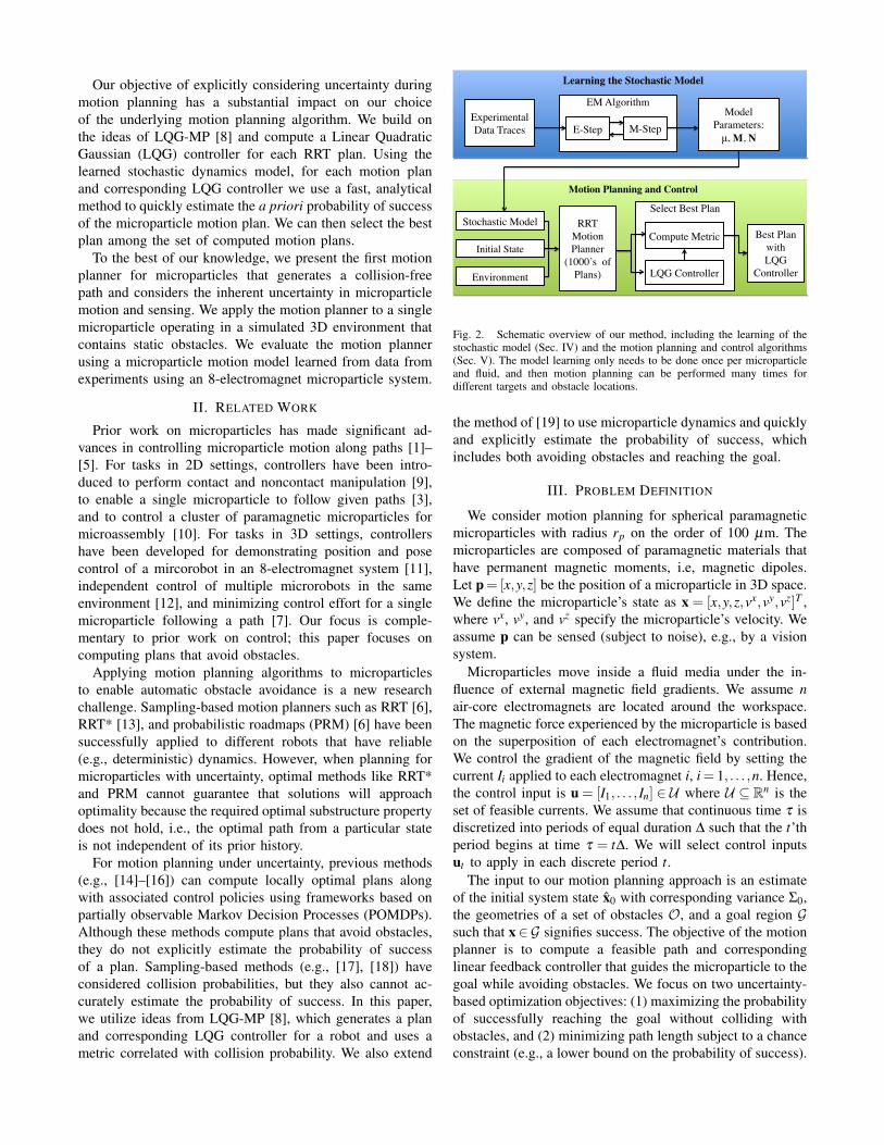
Fig. 2. Schematic overview of our method, including the learning of thestochastic model (Sec. IV) and the motion planning and control algorithms(Sec. V). The model learning only needs to be done once per microparticleand fluid, and then motion planning can be performed many times fordifferent targets and obstacle locations.

the method of [19] to use microparticle dynamics and quicklyand explicitly estimate the probability of success, whichincludes both avoiding obstacles and reaching the goal.

III. PROBLEM DEFINITION

We consider motion planning for spherical paramagneticmicroparticles with radius rp on the order of 100 µm. Themicroparticles are composed of paramagnetic materials thathave permanent magnetic moments, i.e, magnetic dipoles.Let p= [x,y,z] be the position of a microparticle in 3D space.We define the microparticle’s state as x = [x,y,z,vx,vy,vz]T ,where vx, vy, and vz specify the microparticle’s velocity. Weassume p can be sensed (subject to noise), e.g., by a visionsystem.

Microparticles move inside a fluid media under the in-fluence of external magnetic field gradients. We assume nair-core electromagnets are located around the workspace.The magnetic force experienced by the microparticle is basedon the superposition of each electromagnet’s contribution.We control the gradient of the magnetic field by setting thecurrent Ii applied to each electromagnet i, i= 1, . . . ,n. Hence,the control input is u = [I1, . . . , In] ∈ U where U ⊆ Rn is theset of feasible currents. We assume that continuous time τ isdiscretized into periods of equal duration ∆ such that the t’thperiod begins at time τ = t∆. We will select control inputsut to apply in each discrete period t.

The input to our motion planning approach is an estimateof the initial system state x0 with corresponding variance Σ0,the geometries of a set of obstacles O, and a goal region Gsuch that x∈G signifies success. The objective of the motionplanner is to compute a feasible path and correspondinglinear feedback controller that guides the microparticle to thegoal while avoiding obstacles. We focus on two uncertainty-based optimization objectives: (1) maximizing the probabilityof successfully reaching the goal without colliding withobstacles, and (2) minimizing path length subject to a chanceconstraint (e.g., a lower bound on the probability of success).

IV. STOCHASTIC MODEL OF MICROPARTICLE MOTION

For efficient motion planning, we need a discrete-timestochastic model of microparticle motion and sensing. In thissection, we formulate this model and describe how we learnthe uncertainty parameters of the model from data tracesfrom a 3D 8-electromagnet system as outlined in Fig. 2.

A. Modeling Microparticle Dynamics

Microparticles move under the influence of a magneticforce, a drag force, and a buoyancy force. We can controlthe magnetic force by applying currents to the magnetssurrounding the microparticle’s workspace. We define themagnetic force f(p) = [Fx,Fy,Fz]T ∈R3×1, where Fx,Fy,Fz

are the components of f(p) in the x, y, and z directions,respectively. The magnetic force equals:

f(p) =4

3µ0(1+Xm)πr3

pXmuT (∇(BT (p)B(p)))u, (1)

where Xm is the magnetic susceptibility constant, µ0 is thevacuum permeability, and B ∈ R3×n is a matrix definingthe magnetic field that depends on the position where themagnetic force is measured [11]. To compute currents forany desired magnetic force, we utilize a current-force mapthat allows us to invert equation 1 [7]. The gradient ofthe magnetic field is almost a constant in the workspace.Hence, we simply write the magnetic force as f. We requiref ∈ F , where F is the feasible set of control inputs. In ourimplementation, we require |f| ≤ |f|max, where |f|max is themaximum norm of a magnetic force which can be generatedby the system.

The drag force acting on the microparticle is fd =[κvx,κvy,κvz]T ∈ R3×1, where κ = −6πηrp is a constant.We define the net buoyancy force acting on the microparticleas Fb = V (ρb−ρ f )g, where V, ρb, and ρ f are the volumeand density of the microparticle, and the density of fluid,respectively. We also require |v| ≤ |v|max for some maximumfeasible microparticle velocity vmax. Given x(τ) and f(τ) attime τ , we can define the continuous-time dynamics modelof a microparticle as follows:

x(τ) =

vx(τ)vy(τ)vz(τ)

(Fx(τ)+κvx(τ))/m(Fy(τ)+κvy(τ))/m

(Fz(τ)−Fb +κvz(τ))/m

(2)

where m is the mass of the microparticle. We define matrix

A =

[03×3 I3×303×3

κ

m I3×3

]and matrix B =

[03×31m I3×3

]. Hence, the

above continuous-time dynamics can be written as:

x(τ) = Ax(τ)+Bf′(τ) (3)

where f′(τ) = f(τ)+Fb[0,0,−1]T .For purposes of motion planning and microparticle simu-

lation, we need to derive the discrete-time dynamics based onthe above continuous-time dynamics. We first note that f′(τ)can serve as a high level control input for motion planning.

microscopes

?

-

electromagnets6BBBBM

� XXXXX

Xy

workspace@@@R

Fig. 3. Experimental testbed for learning the stochastic model. The systemincludes 8 iron-core electromagnets (only the bottom 4 are shown) thatsurround a 10× 10× 10 mm3 workspace. Inside the workspace we placea reservoir of fluid in which the microparticle can move. The system alsoincludes 2 orthogonally placed microscopes for obtaining images of theworkspace for the purpose of localizing the microparticle.

At any time step t ∈ N of duration ∆, the high level controlinput is defined as:

f′t = [Fxt ,F

yt ,F

zt −Fb]

T , f′t ∈ {f′ | |f′−Fbn| ≤ |f|max}, (4)

where n = [0,0,−1]T . When the high level control input f′tis constant between two successive time steps t and t + 1,the state xt+1 can be computed given xt by solving thedifferential equation 3:

xt+1 = Fxt +Gf′t , (5)with

F = exp(A∆), G =

∫∆

0exp(A(∆− τ))B dτ, (6)

where F and G can be evaluated analytically.To model uncertainty, we assume that at any time step t,

the dynamics is corrupted by additive noise mt drawn froma Gaussian distribution with mean µ ∈ R6×1 and varianceM ∈ R6×6:

xt+1 = Fxt +Gf′t +mt , mt ∼N (µ,M). (7)

The tracking system is able to sense the microparticle’s3D position, and we assume the measurement is corruptedby noise n ∈ R3 where n ∼ N (0,N) for some variance N.This gives us the following sensing model:

zt = h(xt ,n) = Cxt +n, C = [I3×3,03×3]. (8)

The stochastic dynamics and the stochastic sensing modelwill be used to a priori estimate the probability of successof any feasible plan from the planner.

B. Learning the Uncertainty Parameters

In order to estimate the parameters µ , M, and N, we obtaintraces of microparticle motion from a system [7] shown inFig. 3. We recorded K = 4 independent trajectories. For eachtrajectory j, we derived and recorded a sequence of pairs{p j

t ,ujt } where 1 ≤ j ≤ K, 0 ≤ t ≤ Tj, p denotes the 3D

position identified by the vision system, and Tj is the number

of time steps in trajectory j (which was several hundred foreach trajectory). From u j

t we can derive the f′ jt using themodeling in Sec. IV-A.

The actual states x of the microparticle are latent. Similarto [20] except that we do not explicitly assume µ = 0, we usethe Expectation-Maximization (EM) algorithm to learn µ , M,and N from the given data. We summarize the approach next.

a) E-Step: In the E-step, we assume µ , N, and M areknown. For each trajectory j, we use a Kalman smootherto compute the posterior distributions of all latent statesx j

t for 0 ≤ t ≤ Tj. The Kalman smoother computes theGaussian distribution N (x j

t|t ,Σjt|t), which is the distribution

of x jt conditioned on all observations (p j) up to and including

time step t. The Kalman smoother also computes a GaussiandistributionN (x j

t+1|t ,Σjt+1|t), which is the distribution of x j

t+1conditioned on all observations up to and including timestep t. Finally, the Kalman smoother returns the Gaussiandistribution N (x j

t|Tj,Σ j

t|Tj), which is the posterior distribution

of x jt conditioned on all observations in trajectory j.b) M-Step: In the M-step, we assume the posterior

distributions of all latent states x jt are available. We can

model the expected likelihood of the recorded traces as:

Q(µ,M,N) = Ex(logK∏

j=1

Tj∏t=0

P(p jt |x

jt )P(x

jt+1|f

′ jt ,x

jt )), (9)

wherep j

t |xjt ∼ N (Cx j

t ,N), (10)

x jt+1|f

′ jt ,x

jt ∼ N (Fx j

t +Gf′ jt +µ,M). (11)

The expectation is taken with respect to the posterior distri-butions N (x j

t|Tj,Σ j

t|Tj) for 0 ≤ t ≤ T j, 1 ≤ j ≤ K. We max-

imize the expected likelihood Q(µ,M,N) of the recordedtraces with respect to µ , M, and N. We derived closed formupdate rules for updating µ , M, and N by extending theapproach of [20].

We start the E-step with an initial guess of µ , N, and M.We keep iterating the E-step and M-step until convergence.To properly model uncertainty of the microparticle system inour motion planner and simulation results in Sec. VI, we usethe computed values for µ , N, and M in conjunction withthe discrete-time stochastic model in Sec. IV-A.

V. MOTION PLANNING FOR MICROPARTICLES

In this section, we present a motion planner for micropar-ticles that utilizes the stochastic motion and sensing modellearned by the method in Sec. IV-B. As outlined in Fig.2, we utilize RRT to generate a large set of feasible plans.For each feasible plan we compute a corresponding linearfeedback controller (LQG) as in LQG-MP [8]. We thenextend the method in [19] to estimate the probability ofsuccess of each plan for the microparticle. We select thebest plan based on the chosen cost metric (e.g., maximizingprobability of success or minimizing path length subject to achance constraint). Once a plan is selected, we can executethe plan’s corresponding linear feedback controller (LQG) tomove the microparticle along the planned path.

A. Sampling-Based Motion PlanningFor motion planning, we use a rapidly-exploring random

tree (RRT), a well-established sampling-based motion plan-ner that has been successfully used in a wide variety ofapplications [6]. The RRT is rooted at the microparticle’sinitial state x0. At each iteration of the RRT algorithm, wesample a state xsample ∈Q, find its nearest neighbor xnear inthe tree, and compute a feasible control f′ that grows the treefrom xnear toward xsample using the RRT’s “extend” function,i.e., (xnew, f′) = extend(xnear,xsample) where xnew requires nomore than ∆ time to reach from xnear [21]. The RRT’s extendfunction uses the deterministic discrete-time dynamics model(Eq. 7 with mt = µ). The output of the RRT is a nominalmotion plan π = [x◦0, f

′◦0 ,x

◦1, f′◦1 , . . . ,x

◦T , f′◦T ], where T is the

number of time steps and x◦0 = x0. We refer readers to [21]for details on RRT.

Instead of generating motion plans only from a single RRTstructure (which has poor performance for optimization), ourapproach is to simultaneously execute a large number ofindependent RRTs to generate a set of feasible plans andthen select the best plan based on the specified cost metric.

B. LQG Control for a MicroparticleThe RRT planner provides a nominal plan π that satisfies

x◦t+1 = Fx◦t + Gf′◦t + µ , for 0 ≤ t ≤ T − 1. To control themicroparticle along the nominal plan π , we use the LQGcontroller since it provides optimal control for linear Gaus-sian motion and sensor models with a quadratic cost functionpenalizing deviation from the path. The LQG controller usesa Kalman filter for state estimation in conjunction with anLQR control policy [22].

Instead of directly controlling the state itself, we modeldeviation of the state with respect to the plan π . This isreasonable since our goal is to stay close to π . For 0≤ t ≤ T ,we define xt = xt−x◦t , f′t = f′t−f′◦t , and zt = zt−h(x◦t ). Hence,the dynamics model and sensing model for deviations can bemodeled as:

xt+1 = Fxt +Gf′t + mt , mt ∼N (0,M), (12)and

zt = Cxt +nt , nt ∼N (0,N). (13)

In order to penalize deviations from π , we define the costfunction as:

E

(T∑

t=0

xTt Cxt + f′Tt Df′t

). (14)

These are the standard formulations of LQG control [22].During execution, a Kalman filter is used to estimate the

true deviation xt at each time step. We define the estimationof the state deviation at time step t as xt , which can beobtained from the Kalman filter after sensing feedback isreceived. We then use an LQR controller for which wecan compute the feedback matrix Lt for each time step. Asthe true state is unknown, we use the estimate xt from theKalman filter to determine the next optimal control input.The control policy is then:

f′t = f′◦t +Lt xt . (15)The microparticle then will execute f′t at time step t.

C. Optimization Objectives Based on Probability of Success

Both cost metrics (1) maximizing probability of successand (2) minimizing path length subject to a chance constraintrequire a priori estimation of the probability of success ofa motion plan. With the stochastic dynamics and sensingof the microparticle, we extend the method in [19] to apriori estimate the probability of success of a feasible motionplan. This method a priori estimates the probability ofcollision of a motion plan assuming that a correspondingLQG controller is used during execution. Given a nominalplan π , [x0, f′0, . . . ,xT , f′T ], and an initial beliefN (x0, Σ0), wecompute a sequence of Gaussian distributions {N (xt , Σt)},for 0 ≤ t ≤ T . This sequence of Gaussian distributionscaptures the distributions of deviations from π during theexecution of the plan with the LQG feedback controller.

To compute Pc, the estimated probability of collision, weuse the method in [19]. At time step t, let us assume the stateof the microparticle is xt ∼N (xt , Σt). Before propagating tothe time step t + 1, we truncate this Gaussian distributionagainst obstacles to remove the parts of the distribution thatcollide with obstacles. The truncated distribution capturesthe possible states of the microparticle that are collision-free at time step t. By propagating the truncated distributionto time step t + 1, we only propagate to the next time stepstates that are collision-free. Hence, we properly consider thedependency of uncertainty on previous time steps. Namely,the possible states of the microparticle at time step t + 1should be conditioned on the fact that the microparticle iscollision-free at time step k, where 0≤ k ≤ t.

We also need to estimate the probability that the mi-croparticle reaches the goal region at the last time step.Given the belief of the microparticle at the last time stepxT ∼N (xT , ΣT ), we can compute the probability of reachingthe goal region as:

Pg =

∫p∈G

exp(− 12 (p−ΛxT )

T (ΛΣT ΛT )−1(p−ΛxT ))√(2π)3|ΛΣT ΛT |

dp,

(16)where G is the goal region and Λ = [I3×3,03×3]. In ourimplementation, we numerically estimate Eq. 16.

The probability of success can be computed as Ps =(1−Pc)Pg. Using the computations described above, we canevaluate the probability of success for each feasible plan andselect the best plan based on the chosen cost metric.

VI. EVALUATION

We apply our motion planner in simulation to a micropar-ticle moving in a 3D environment which contains multipleobstacles and a goal region. We evaluate our method fortwo cost metrics: (1) maximizing probability of success, and(2) minimizing path length subject to a chance constraint.We define a chance constraint as Ps ≥ Ps, where 0≤ Ps ≤ 1is specified by the user. The chance constraint imposes alower bound on the probability of success (i.e., avoidingobstacles and reaching the goal region). We tested our C++implementation on a PC with a 3.7 GHz Intel Core i7processor.

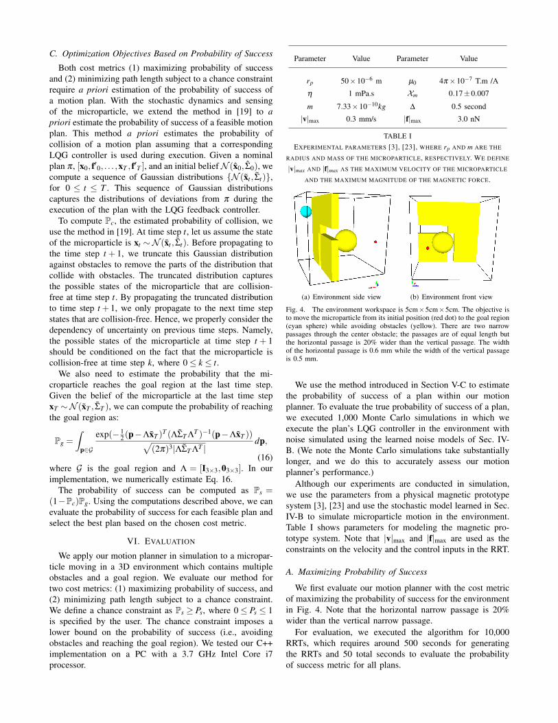
Parameter Value Parameter Value

rp 50×10−6 m µ0 4π×10−7 T.m /A

η 1 mPa.s Xm 0.17±0.007

m 7.33×10−10kg ∆ 0.5 second

|v|max 0.3 mm/s |f|max 3.0 nN

TABLE IEXPERIMENTAL PARAMETERS [3], [23], WHERE rp AND m ARE THE

RADIUS AND MASS OF THE MICROPARTICLE, RESPECTIVELY. WE DEFINE

|v|max AND |f|max AS THE MAXIMUM VELOCITY OF THE MICROPARTICLE

AND THE MAXIMUM MAGNITUDE OF THE MAGNETIC FORCE.

(a) Environment side view (b) Environment front view

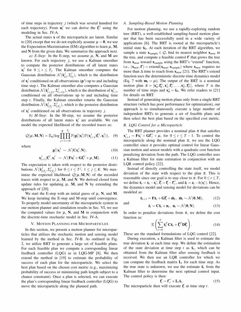
Fig. 4. The environment workspace is 5cm×5cm×5cm. The objective isto move the microparticle from its initial position (red dot) to the goal region(cyan sphere) while avoiding obstacles (yellow). There are two narrowpassages through the center obstacle; the passages are of equal length butthe horizontal passage is 20% wider than the vertical passage. The widthof the horizontal passage is 0.6 mm while the width of the vertical passageis 0.5 mm.

We use the method introduced in Section V-C to estimatethe probability of success of a plan within our motionplanner. To evaluate the true probability of success of a plan,we executed 1,000 Monte Carlo simulations in which weexecute the plan’s LQG controller in the environment withnoise simulated using the learned noise models of Sec. IV-B. (We note the Monte Carlo simulations take substantiallylonger, and we do this to accurately assess our motionplanner’s performance.)

Although our experiments are conducted in simulation,we use the parameters from a physical magnetic prototypesystem [3], [23] and use the stochastic model learned in Sec.IV-B to simulate microparticle motion in the environment.Table I shows parameters for modeling the magnetic pro-totype system. Note that |v|max and |f|max are used as theconstraints on the velocity and the control inputs in the RRT.

A. Maximizing Probability of Success

We first evaluate our motion planner with the cost metricof maximizing the probability of success for the environmentin Fig. 4. Note that the horizontal narrow passage is 20%wider than the vertical narrow passage.

For evaluation, we executed the algorithm for 10,000RRTs, which requires around 500 seconds for generatingthe RRTs and 50 total seconds to evaluate the probabilityof success metric for all plans.

(a) Maximizing probability ofsuccess

(b) LQG control of the plan withhighest probability of success

(c) Maximum Clearance (d) LQR control of the plan withmaximum clearance

Fig. 5. Our method computes a motion plan and corresponding con-troller with the objective of maximizing probability of success. For thisenvironment, we show the computed nominal plan (green trajectory) (a).The red ellipses show the Gaussian distributions that capture the deviationsof states along the nominal motion plan. We also show an examplesuccessful execution of LQG control (blue trajectory) along the nominalplan (b). The plan computed with the maximum clearance metric passesthrough the horizontal passage, which is wider than the vertical passagebut not aligned with the microparticle’s uncertainty (c). When executinga maximum clearance trajectory using the corresponding LQR controller,the microparticle is more likely to collide with an obstacle (blue exampleexecution) (d) than when using the probability of success metric.

Fig. 5(a) shows the motion plan computed for maximizingthe probability of success. The plan is shown in green, andthe red ellipses show the estimated uncertainty distributionin position (3 standard deviations) at several time steps alongthe path. The estimated probability of success for the selectedplan (using the fast analytical methods in Sec. V-C) is 96.1%.The true probability of success from Monte Carlo simulationsis 99.6%. In Fig. 5(b) we illustrate an example execution ofthe LQG controller along the planned path while subject tonoise from the model learned in Sec. IV-B.

To maximize the probability of success, the microparticlepasses through the vertical passage. Although the horizontalpassage is wider, the uncertainty model learned in Sec. IV-Bhas higher uncertainty in the Z direction, likely due to noisein the buoyancy force. The impact of the extra uncertaintycan be seen in red ellipses in Fig. 5(a). Thus, it is safer topass through the narrower vertical passage.

We compare our motion planning results using the proba-bility of success metric to using a classical cost metric that isalso related to safe motion planning: maximizing clearancein conjunction with an LQR controller, which does notrequire stochastic model learning (Sec. IV-B) or probabilityof success estimation (Sec. V-C). Fig. 5(c) shows the motion

(a) Initial environment (b) Optimal plans for differentcost metrics

Fig. 6. We evaluate the motion planner for cost metrics related to shortestpaths in this environment (a) where the objective is to move the microparticlefrom its initial position (red dot) to the goal region (cyan sphere) whileavoiding obstacles (yellow). We show (b) the computed plans for three costmetrics: minimizing path length (black), minimizing path length subjectto C1 (red), minimizing path length subject to C2 (green) and maximizingclearance (blue).

plan computed for maximizing clearance from obstacles. Tomaximize clearance, the microparticle passes through thehorizontal passage since it is wider. However, the largeruncertainties along the Z direction affect the probability ofsuccess. As shown in Fig. 5 (c), the uncertainty ellipses col-lide with the obstacles while passing through the horizontalpassage. In addition, the cost metric of maximizing clearanceaims for the goal region but does not explicitly consider thelikelihood that the microparticle will end up inside the goalregion due to uncertainty. The impact of these factors is thatthe true probability of success of the maximum clearanceplan is 91%, substantially lower than the plan that explicitlymaximizes probability of success.

B. Shortest Path Subject to a Chance Constraint

We also evaluated our method on another cost metric:minimizing path length subject to a chance constraint. Weconsider two chance constraints: C1: Ps ≥ 0.99 and C2: Ps ≥0.90. We compare to two classical cost metrics: minimizingpath length and maximizing clearance, which are both usedin conjunction with an LQR controller and do not requirethe stochastic model learning (Sec. IV-B) or probability ofsuccess estimation (Sec. V-C).

For evaluation, we executed the algorithm for 20,000RRTs, which required around 200 seconds for generatingthe RRTs and 160 total seconds to evaluate the probabilityof success metric for all plans. As before, for shortest pathand maximizing clearance, the true probability of success isevaluated using Monte Carlo simulations with LQR control.

Fig. 6 shows the results of using four different costmetrics. The black plan from minimizing path length alsopasses closest to an obstacle (the left cylinder in Fig. 6(b)).The red plan is the plan that moves furthest from theobstacle, such that it can satisfy C1 : Ps ≥ 0.99. The blueplan for maximizing clearance passes through the middle ofthe narrow passage to achieve the largest clearance.

Table II shows the statistics for the four different costmetrics. As we can see, although the shortest path cost metric

Cost Metric Length (mm) Clearance (mm) Pest Ptrue

Shortest Path 5.66 0.02 / 37.9%

Max Clearance 6.70 0.53 / 86.9%

Shortest Path s.t C2 5.79 0.12 94.0% 95.9%

Shortest Path s.t C1 5.84 0.22 99.9% 99.8%

TABLE IISTATISTICS FOR FOUR COST METRICS. WE DENOTE Pest AS THE

ESTIMATED PROBABILITY OF SUCCESS AND Ptrue AS THE TRUE

PROBABILITY OF SUCCESS. LQR CONTROL IS APPLIED TO SHORTEST

PATH AND MAX CLEARANCE METRICS. C1 STANDS FOR Ps > 0.99 AND

C2 STANDS FOR Ps > 0.9.

finds the shortest path, it passes too close to the obstacles(clearance equals to 0.02 mm) to achieve a reasonable prob-ability of success. On the other hand, our method using theshortest path subject to a chance constraint generates plansthat enforce a minimum probability of success requirement.For a less restrictive chance constraint (C2), we find a shorterpath but with smaller probability of success. Compared tomaximizing clearance, our method indeed not only finds ashorter path, but also achieves higher probability of success.This is because the cost metric of maximizing clearance doesnot explicitly consider the likelihood of reaching the goal.Our method can compute short paths while still maintaininghigh probability of success.

VII. CONCLUSION

In this paper, we introduced a motion planner to guidea spherical paramagnetic microparticle to a target whileavoiding obstacles. The motion planner computes a pathand a corresponding controller for the electromagnets’ cur-rents. Our motion planner explicitly considers uncertainty inthe microparticle’s motion; we formalized and utilized costmetrics that consider the probability that the microparticleavoids obstacle collisions and reaches the target. To enableeffective consideration of uncertainty, our cost metrics reliedon a stochastic model of the uncertainty in motion andsensing. The stochastic model was learned from experimentsconducted in a 3D 8-electromagnet microparticle testbed.

We applied the motion planner in a simulated 3D en-vironment with static obstacles and demonstrated that thecomputed plans are more likely to result in task success thanplans based on traditional metrics such as shortest path ormaximum clearance. In future work, we plan to integrate themotion planner with a 3D paramagnetic microparticle systemto further evaluate algorithm performance. We also plan toinvestigate extending the motion planner to properly handleenvironments with moving obstacles.

VIII. ACKNOWLEDGMENT

The authors thank Bart Reefman for providing inputregarding the experimental setup.

REFERENCES

[1] J. J. Abbott, Z. Nagy, F. Beyeler, and B. J. Nelson, “Robotics in thesmall, part I: microbotics,” IEEE Robotics and Automation Magazine,vol. 14, no. 2, pp. 92—-103, Jun. 2007.

[2] M. Sitti, “Microscale and nanoscale robotics systems: characteristics,state of the art, and grand challenges,” IEEE Robotics and AutomationMagazine, pp. 53–60, Mar. 2007.

[3] I. S. M. Khalil, J. D. Keuning, L. Abelmann, and S. Misra, “Wire-less magnetic-based control of paramagnetic microparticles,” Proc.IEEE RAS/EMBS Int. Conf. Biomedical Robotics and Biomechatronics(BioRob), pp. 460–466, Jun. 2012.

[4] B. J. Nelson, I. K. Kaliakatsos, and J. J. Abbott, “Microrobots for min-imally invasive medicine,” Annual Review of Biomedical Engineering,vol. 12, pp. 55–85, Aug. 2010.

[5] M. Sitti, “Voyage of the microrobots,” Nature, vol. 458, pp. 1121–1122, Apr. 2009.

[6] S. M. LaValle, Planning Algorithms. Cambridge, U.K.: CambridgeUniversity Press, 2006.

[7] I. S. M. Khalil, R. M. P. Metz, B. A. Reefman, and S. Misra,“Magnetic-based minimum input motion control of paramagneticmicroparticles in three-dimensional space,” in Proc. IEEE/RSJ Int.Conf. Intelligent Robots and Systems (IROS), Nov. 2013, pp. 2053–2058.

[8] J. van den Berg, P. Abbeel, and K. Goldberg, “LQG-MP: Optimizedpath planning for robots with motion uncertainty and imperfect stateinformation,” Int. J. Robotics Research, vol. 30, no. 7, pp. 895–913,Jun. 2011.

[9] C. Pawashe, S. Floyd, E. Diller, and M. Sitti, “Two-dimensionalautonomous microparticle manipulation strategies for magnetic micro-robots in fluidic environments,” IEEE Trans. Robotics, vol. 28, no. 2,pp. 467–477, Apr. 2012.

[10] I. Khalil, F. Brink, O. S. Sukas, and S. Misra, “Microassembly usinga cluster of paramagnetic microparticles,” in Proc. IEEE Int. Conf.Robotics and Automation (ICRA), May 2013, pp. 5507–5512.

[11] M. P. Kummer, J. J. Abbott, B. E. Kratochvil, R. Borer, A. Sengul,and B. J. Nelson, “OctoMag: An electromagnetic system for 5-DOFwireless micromanipulation,” IEEE Trans. Robotics, vol. 26, no. 6, pp.1006–1017, Dec. 2010.

[12] E. Diller, J. Giltinan, and M. Sitti, “Independent control of multiplemagnetic microrobots in three dimensions,” Int. J. Robotics Research,vol. 32, no. 5, pp. 614–631, May 2013.

[13] S. Karaman and E. Frazzoli, “Sampling-based algorithms for optimalmotion planning,” Int. J. Robotics Research, vol. 30, no. 7, pp. 846–894, Jun. 2011.

[14] R. Platt Jr., R. Tedrake, L. Kaelbling, and T. Lozano-Perez, “Be-lief space planning assuming maximum likelihood observations,” inRobotics: Science and Systems, 2010.

[15] M. P. Vitus and C. J. Tomlin, “Closed-loop belief space planningfor linear, Gaussian systems,” in Proc. IEEE Int. Conf. Robotics andAutomation (ICRA), May 2011, pp. 2152–2159.

[16] J. van den Berg, S. Patil, and R. Alterovitz, “Motion planning underuncertainty using iterative local optimization in belief space,” Int. J.Robotics Research, vol. 31, no. 11, pp. 1263–1278, Sep. 2012.

[17] A. Bry and N. Roy, “Rapidly-exploring random belief trees for motionplanning under uncertainty,” in Proc. IEEE Int. Conf. Robotics andAutomation (ICRA), May 2011, pp. 723–730.

[18] S. Prentice and N. Roy, “The belief roadmap: Efficient planning inbelief space by factoring the covariance,” Int. J. Robotics Research,vol. 31, pp. 1263–1278, Sep. 2009.

[19] S. Patil, J. van den Berg, and R. Alterovitz, “Estimating probabilityof collision for safe motion planning under Gaussian motion andsensing uncertainty,” in Proc. IEEE Int. Conf. Robotics and Automation(ICRA), May 2012, pp. 3238–3244.

[20] A. Coates, P. Abbeel, and A. Ng, “Learning for control from multipledemonstrations,” in Proc. Int. Conf. Machine Learning (ICML), 2008,pp. 144–151.

[21] S. M. LaValle and J. J. Kuffner, “Rapidly-exploring random trees:Progress and prospects,” in Algorithmic and Computational Robotics:New Directions, B. R. Donald and Others, Eds. Natick, MA: AKPeters, 2001, pp. 293–308.

[22] D. P. Bertsekas, Dynamic Programming and Optimal Control, 2nd ed.Belmont, MA: Athena Scientific, 2000.

[23] I. S. M. Khalil, R. M. P. Metz, L. Abelmann, and S. Misra, “Inter-action force estimation during manipulation of microparticles,” Proc.IEEE/RSJ Int. Conf. Intelligent Robots and Systems (IROS), pp. 950–956, Oct. 2012.