motion control and simulation of a towing tank … · trailer of towing tank is the basic equipment...

International Journal of Applied Science and Technology Vol. 7, No. 4, December 2017

59

Motion Control and Simulation of a Towing Tank system in an Experimental Water Pool*

Min Xiao

College of Computer and Information Technology

China Three Gorges University

Yichang, 443002, China

Abstract

The underwater towed system is extensively used for various oceanic applications and military tasks etc., it is an

important problem in the design and application of towed system to study its motion characteristics and control

problems. It has very important meanings in the design and use of towed systematic to hold the law and

characteristic of the systematic movement accurately. Trailer of towing tank is the basic equipment which is used

for performance test of ship, and which role is to drag ship model or others for uniform motion in the tank, to

measure the relevant performance parameters of ship after speed stable, to prediction and validation of the merits

or inferiors of hull form design. As trailers uniform model accuracy directly affects the velocity and the accuracy

of test results, which must be equipped with good speed control system which has high precision and immunity in

order to ensure tow-speed precision movement. In this paper, through the establishment of a rigorous theoretical

model, the object study is systematically analyzed and simulated by numerical simulation. The whole process of

the design and simulation of the trailer movement control system is completed. The study of this paper lays the

foundation for the development of successful underwater towing system for laboratory model test and offshore

field prototype test.

Keywords: Towed system, resistance calculation, anti-skid analysis, process segment, speed control, position

control

1. Introduction

An aquatic towing system is an effective method to carry scientific measuring equipment for aquatic search

activities and military reconnaissance. In this study, a controllable aquatic towing system in a test water pool that

meets task requirements and is practical was designed and developed. Based on the simulation of the motion

control of the aquatic towing system in a test water pool, the calculation of the driving power of the trailer for the

test object and the design control strategy for the trailer system velocity and position were analyzed. The results

meet the requirements of the motion parameters of the test object. To research the systematic hydrodynamic

performance, to set up one comparatively perfect simulation system to simulate various kinds of movement and

make use of simulation system to adjust the design project of the towed system, is of great advantage to design

and research towed system, it can save a large amount of time and fund, and avoid the enormous losses of

manpower and material resources.

2. System overview

The primary function of a towing-test water pool is to accommodate the towed paths of a test object in different

positions while measuring various motion parameters of the test object, such as resistance coefficient and position

derivative. A sketch of the towing water pool is shown in Fig.1.

*This work was supported by China Three Gorges University Science Foundation(No. 1311039)

ISSN 2221-0997 (Print), 2221-1004 (Online) © Center for Promoting Ideas, USA www.ijastnet.com

60

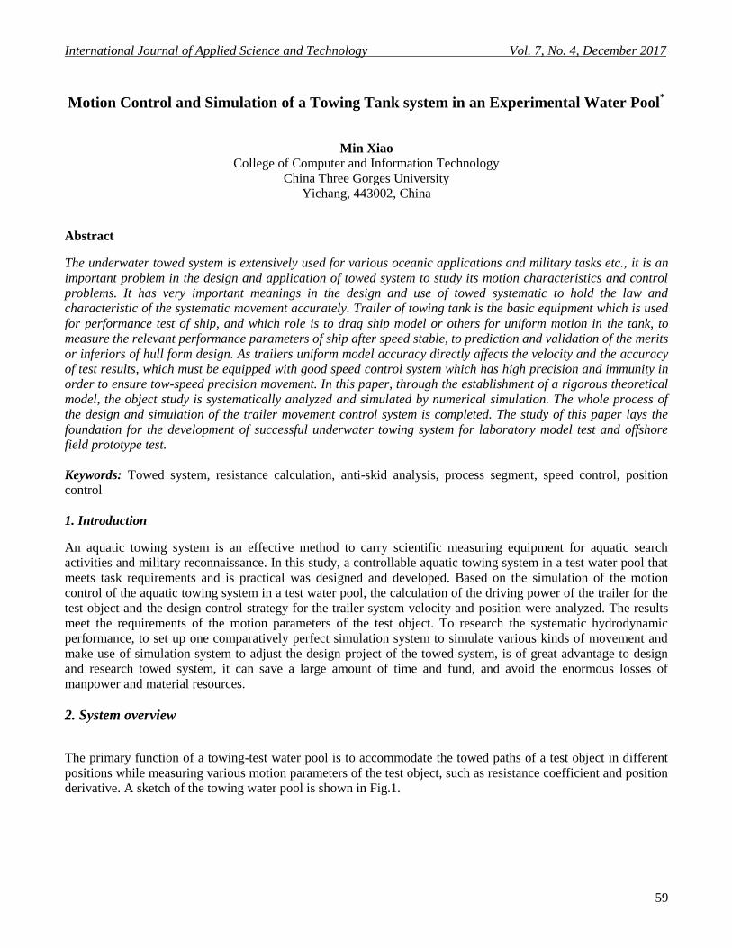
Fig.1Components and layout of the non-standard equipment in the towing water pool

The towing test area consists primarily of a 170m (length, including dock) 7m (water surface width) 6m (water

depth) towing water pool and model installation dock. The trailer, which is installed across the pool on tracks at

both sides of the water pool, drags the test object and acts as a test platform. A trailer motor drives the motion of

the wheel along the tracks. The trailer is8m long and 7.5m wide. The trailer motion is as follows. The trailer

control system starts up and accelerates the trailer. When the trailer reaches the specified test velocity (the

maximum velocity is 7 /m s ), acceleration stops and the trailer moves at a constant velocity. After a period of

constant velocity, the test system is started. When the test is completed, the control system is activated to

decelerate the trailer and stop the motion. The trailer is returned to dock, at which time the test is completed. The

trailer, with a dead weight of 20t (excluding the test object), is supported by 4 wheels, bearing the weight

equally. The trailer is driven by the 4 wheels synchronously. Each wheel is driven by a servo motor. The wheels

are fabricated with hard steel; the track is fabricated with steel. The friction between the wheel and the track is

modeled as steel-steel friction. The wheel diameter is 600mm . The wheel axis and the motor axis are connected

via a straight gear decelerator with a deceleration ratio equal to 8 and a motor rotation rate equal to1500rpm . An

aircraft model, the test object, is installed at the bottom of the trailer via a connector (no longer than 2m ),

completely submerged in water and moving in tandem with the trailer.

The following are the relevant parameters: the test length is 7m ; the test apparatus weight is1.5t ; the drainage

capability is1.5t ; the underwater weight is 0 ; the underwater resistance is 2= xF A Vwat er, where V is the trailer

velocity; and the overall maximum resistance coefficient of the model is 36xA . The trailer has a truss-like

structure; hence, windward resistance to motion should be taken into account. Windward resistance is calculated

by 2=CxF Vwi nd, where V is the trailer velocity, and the overall trailer windward resistance coefficient is 15xC . The

following are the trailer motion parameters: the maximum velocity is 7 /m s ; the maximum acceleration is 20.7 /m s ;

and the maximum deceleration is 22.0 /m s (hydraulic pressure track brake deceleration).

3. Slip and power torque calculation

Based on the conditions provided by the system, the maximum motor power and the maximum torque during

trailer motion are calculated. During motion, dynamic underwater resistance and windward resistance should be

considered. The specified test velocity, acceleration and deceleration should be reached, and wheel slip should not

occur. Slip is related to two factors: The slip friction between the track and the wheel is related to the materials of

both the wheel and the track, as well as to environmental factors, such as humidity, grease pollution and corrosion

level. The tractive force is related to the motor power. The motor has limited power, and its acceleration and

deceleration properties are also fixed. The maximum value of the tractive force is limited by the wheel maximum

adhesive force, i.e., the maximum static friction. The occurrence of slip depends on whether the motion resistance

is greater than the maximum adhesive force (maximum static friction) determined by the wheel pressure.


61

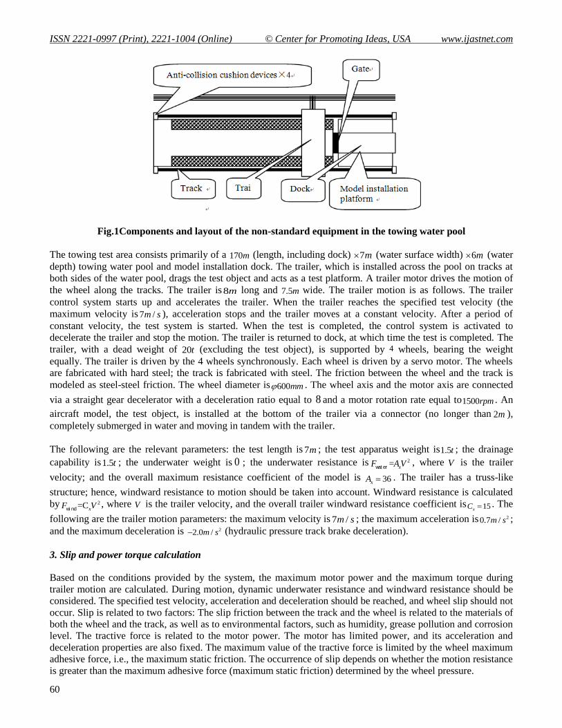
During motion, the trailer is affected by three different forces: the tractive force F , which results in trailer

acceleration; the overall trailer pressure on the track Fn; the trailer is a truss-like structure, whose windward

resistance is 2=CxF Vwi nd, underwater resistance is 2= xF A Vwat er

, and friction is Ff r i ct i on. A simple model of the overall

motion of the trailer from stress is shown in Fig. 2.

Fig. 2 Simplified diagram for overall trailer motion stress model During trailer acceleration, the tractive

force accelerationF is as follows:

= + +F F F F maaccel er at i on wat er wi nd f r i ct i on (1)

When the trailer is moving at a constant velocity, the tractive force Fconstant is as follows:

tan = + +cons tF F F Fwat er wi nd f r i ct i on (2)

When the trailer is decelerating, the brake force Fdeceleration is as follows:

= + + -F F F F maaccel er at i on wat er wi nd f r i ct i on (3)

In the above formulae, waterF is the underwater resistance,

windF is the air resistance, Ff r i ct i on is the rolling friction,

m is the mass, and a is the acceleration. The rolling friction Ff r i ct i on is normally measured using the resistance

moment, a quantity determined by the properties, the surface shape and the weight of the rolling object. Rolling

friction is a moment that hinders rolling. When an object rolls on a coarse plane, if no kinetic force or kinetic

moment is applied, its motion will gradually decrease until it stops. During this process, the rolling object is

affected by gravity and elasticity; the contact point is also affected by static friction.

Existing parameters are fully utilized to obtain a more accurate calculation. The wheel diameter is 600mm , the

wheel axis and the motor axis are connected via a straight gear decelerator, whose deceleration ratio is 8 and

motor rotation rate is1500rpm . The overall trailer pressure on the track is Fn, k is the rolling friction coefficient,

M is the moment, and R is the wheel radius. Based on the following relation:

M=k nF F R r ol l i ng

and then /nF k F R r ol l i ng

Based on the known test conditions, 0.3R m and 20000 9.8 196000nF N . The rolling friction coefficient for steel-

steel is set to 0.005k , then the rolling friction frictionF is as follows:

(0.005 196000) / 0.3 3266.67F N N r ol l i ng

If slip friction is not negligible, the friction coefficient can be adjusted properly to account for slip.

During the acceleration, the rolling wheel has a temporary change from slip to rolling. If system slip is not

allowed, then the relation is as follows:

wind water slip wind water slip+ + + + +F F F F mg F F F (4)

During the acceleration of the trailer, if slip is not allowed, then the force on the trailer is as follows:

wind water slip( + + )F F F F ma mg anda g

http://baike.baidu.com/view/36869.htm


62

It is assumed that the track and the wheel are not corroded and are clean and dry; the steel-steel slip friction

coefficient is calculated via 0.15 .Therefore, the maximum acceleration during the acceleration is as follows:

When 2

1 0.15 9.8 1.47 /a g m s , 0.15

When 2

1= =0.1 9.8=0.98 /a g m s , 0.1

Hence, when the maximum acceleration is 20.7 /m s , trailer slip will not occur.

During constant velocity, there is + +F F F Fconst ant wi nd wat er sl i p, so slip will not occur.

During deceleration, there are occurrences of slip with a brake force and without a brake force; however, to

prevent system slip, the brake force'F should satisfy the following:

'

wind water slip0< + + =F F F F ma mg and: a g

Therefore, under the aforementioned parameters, the maximum theoretical deceleration range is as follows: 2

1 0.15 9.8 1.47 /a g m s

The data showed that based on the control strategy requirement, within the system required range of maximum

acceleration 20.7 /m s and maximum deceleration of 22.0m/s , system slip will not occur.

Because the deceleration process uses a hydraulic pressure track brake deceleration, the system brake force is 0.

To prevent system slip, the system resistance should be less than the maximum system static friction, i.e., the

system slip friction, as follows:

wind water slip0< + +F F F mg

During system deceleration, if there is no slip, the resultant force is as follows:

wind water slip+ +ma F F F mg thus: a g

Therefore, under the aforementioned parameters, the maximum theoretical deceleration range during deceleration

is as follows: 2

1 0.15 9.8 1.47 /a g m s

Based on the system requirements and the above analysis, the towing system motion plan is as follows. During

the acceleration phase, the system accelerates at a constant rate 2

1 0.7 /a m s . When the maximum velocity maxV is

reached, the velocity of the trailer is held constant for 12s .The trailer then decelerates at a constantrate 2

2 1.47 /a m s . This relation is described as follows:

2 2

1 1 max 2 2

max 1 1 2 2

1 112 120

2 2a t V a t

V a t a t

Combining the above two formulae with the parameters yields the following:

1

2

max

9.1339( )

4.3495( )

6.3937( / )

t s

t s

V m s

In summary, the system motion strategy is as follows. During acceleration, the trailer accelerates at a constant rate

of 20.7 /m s for9.1339s . After reaching a maximum velocity of6.3937 /m s , the trailer continues at a constant velocity

for12s . The trailer then decelerates at a constant rate of 21.47 /m s for 4.3495s until the system motion stops. The

stroke for the entire process is119.8291m .

According to the formula for motor power, P FV , when F and V are maximum values, power P is also a

maximum. For example, assume that velocity V is at its maximum value. As long as acceleration a is also at its

maximum value, F is also at a maximum value. Whenmax 7 /V m s , there are two scenarios for acceleration:

2

1 0.7 /a m s during trailer acceleration and 2

2 1.47 /a m s during deceleration. The data show that the tractive force

F during trailer acceleration is greater than the tractive force F during deceleration. Therefore, when the trailer

velocity is6.3937 /m s and the acceleration is 20.7 /m s , i.e., when the trailer accelerates from a maximum velocity of 20.7 /m s to a maximum velocity of 6.3937 /m s , the tractive force F at this moment is the maximum F; the motor

power reaches its maximum value also.


63

2

max 51 6.3937 20000 0.7 3266.67 19351.51938419F N

The maximum power is as follows:

max max max 19351.51938419 6.3937 123.7278P F V KW The maximum torque is the following:

max max9550 /T P n

where n is the motor rotation rate, 1500n rpm .

Hence, the maximum torque is as follows:

max 9550 123.7278/1500 787.7337 MT N

4. Accurate control of velocity and position at transition segments

The process of start, acceleration, stabilization, deceleration and stop should be completed in the stroke range of

120m ; slip should not occur during acceleration and deceleration. Acceleration should notexceed 20.7 /m s ;

maximum deceleration should not exceed 22.0 /m s (hydraulic pressure track brake deceleration); and the

maximum velocity is 7 /m s . After accelerating to the maximum velocity, the trailer is stabilized for1s . Then, the

trailer moves at a constant velocity for 10s to perform object testing. When the test is complete, the trailer

continues at a constant velocity for1s . Next, the deceleration starts, continuing until the trailer stops.

Velocity stability requirements: When the velocity is less than1 /m s , the velocity fluctuations should be less than

0.3% . When the velocity is greater than or equal to1 /m s , the velocity fluctuations should be less than0.1% .

Finally, the maximum velocity is 7 /m s .Based on requirements above, the strategy for the trailer motion is

designed, which includes the motion stroke distribution at acceleration, the stabilization, the deceleration segment,

the variable or constant acceleration and the deceleration strategy.

When the motion stroke is greater than 10m and the average velocity is 3.5 /m s , the positioning accuracy should

be ≤ 5 mm; When the motion stroke is less than 10m and the duration of the motion is less than 8 seconds, the

positioning accuracy shouldbe ≤ 5 mm;During the positioning and movement of the trailer, overshoot should not

occur. Based on requirements above, the strategy for the trailer motion is designed, which includes the motion

stroke distribution at acceleration, the stabilization, the deceleration segment, the variable or constant acceleration

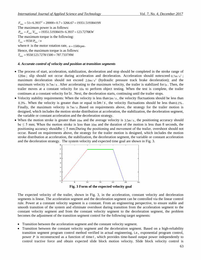
and the deceleration strategy. The system velocity and expected time goal are shown in Fig. 3.

Fig. 3 Form of the expected velocity goal

The expected velocity of the trailer, shown in Fig. 3, in the acceleration, constant velocity and deceleration

segments is linear. The acceleration segment and the deceleration segment can be controlled via the linear control

rule. Power at a constant velocity segment is a constant. From an engineering perspective, to ensure stable and

smooth transition of the system and eliminate overshoot during transition from the acceleration segment to the

constant velocity segment and from the constant velocity segment to the deceleration segment, the problem

becomes the adjustment of the transition segment control for the following target segments:

Transition between the acceleration segment and the constant velocity segment.

Transition between the constant velocity segment and the deceleration segment. Based on a high-reliability

transition segment program control method verified in actual engineering, i.e., exponential program control,

power P is reconstructed as a function of time t , which provides time-based output power independently to

control tractive force and obtain expected slide block motion velocity. Slide block velocity control is


64

performed via the following control mode: P F V

The tractive force is controlled by controlling power and eventually to achieve the expected goal of controlling

velocity. However, further analysis shows that ,P V F V are both functions ofV . Therefore, when conventional

feedback control is applied, the situation shown in Fig. 4 will occur.

Fig. 4 Feedback diagram for velocity control rule

As velocity V is both a control variable and a control parameter, a closed-loop coupling state is formed, which

will eventually become a control loop. Therefore, decoupling is required. Because motor control is essential to

control motor output power, the parameterization of motor output power is redesigned. Analytic methods and

dynamic decoupling methods are employed. When these methods are applied to program control of an aircraft

transition segment, exponential program control is employed to reconstruct power P as a function of time t ,

which provides time-based output power independently to control tractive force and obtain expected slide block

velocity.

The general expression for the program control rule for the relation between power and time is as follows:

P f t

The formula for the velocity-time function during acceleration is as follows:

1 1 (0 9.1339)v a t t

The formula for the velocity-time function during the constant velocity period is as follows:

2 6.3937 (9.1339 21.1339)v t t

The formula for the velocity-time function during deceleration is:

3 26.3937 ( 21.1339)(21.1339 25.4834)v a t t

To ensure smooth and stable function transition in each segment, parameterization design for these functions in

the form of time domain step function is as follows:

2

2

2

5

( 9.5)

5 3.6

( 20.5)

5 3.58^2

5

1.2373 10 8.89.1339

1.2373 10 8.8 9.5

34216 9.5 20.5

1.5376 10 20.5 21.4

1 ( 21.1339)1.5376 10 21.4 25.4834

4.3495

t

t

tP t

P e t

P t

P e t

tP t

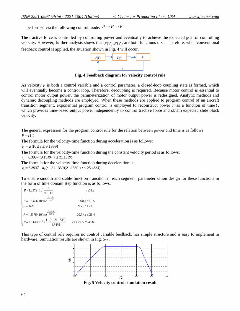
This type of control rule requires no control variable feedback, has simple structure and is easy to implement in

hardware. Simulation results are shown in Fig. 5-7.

Fig. 5 Velocity control simulation result


65

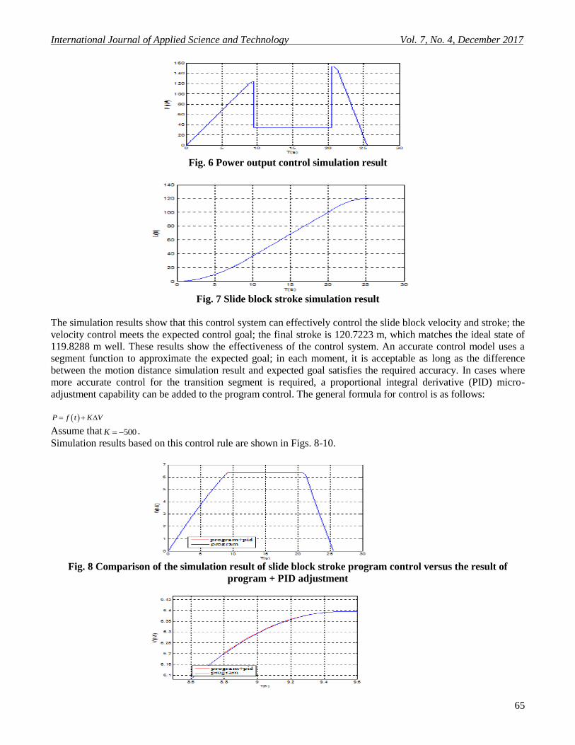
Fig. 6 Power output control simulation result

Fig. 7 Slide block stroke simulation result

The simulation results show that this control system can effectively control the slide block velocity and stroke; the

velocity control meets the expected control goal; the final stroke is 120.7223 m, which matches the ideal state of

119.8288 m well. These results show the effectiveness of the control system. An accurate control model uses a

segment function to approximate the expected goal; in each moment, it is acceptable as long as the difference

between the motion distance simulation result and expected goal satisfies the required accuracy. In cases where

more accurate control for the transition segment is required, a proportional integral derivative (PID) micro-

adjustment capability can be added to the program control. The general formula for control is as follows:

P f t K V

Assume that 500K .

Simulation results based on this control rule are shown in Figs. 8-10.

Fig. 8 Comparison of the simulation result of slide block stroke program control versus the result of

program + PID adjustment


66

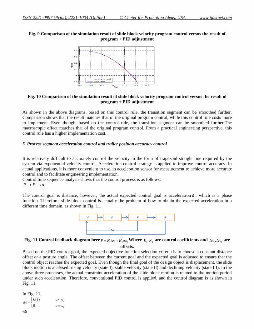
Fig. 9 Comparison of the simulation result of slide block velocity program control versus the result of


Fig. 10 Comparison of the simulation result of slide block velocity program control versus the result of


As shown in the above diagrams, based on this control rule, the transition segment can be smoothed further.

Comparison shows that the result matches that of the original program control, while this control rule costs more

to implement. Even though, based on the control rule, the transition segment can be smoothed further.The

macroscopic effect matches that of the original program control. From a practical engineering perspective, this

control rule has a higher implementation cost.

5. Process segment acceleration control and trailer position accuracy control

It is relatively difficult to accurately control the velocity in the form of trapezoid straight line required by the

system via exponential velocity control. Acceleration control strategy is applied to improve control accuracy. In

actual applications, it is more convenient to use an acceleration sensor for measurement to achieve more accurate

control and to facilitate engineering implementation.

Control time sequence analysis shows that the control process is as follows:

P F a

The control goal is distance; however, the actual expected control goal is acceleration a , which is a phase

function. Therefore, slide block control is actually the problem of how to obtain the expected acceleration in a

different time domain, as shown in Fig. 11.

Fig. 11 Control feedback diagram here

1 1 2 2F K x K x Where 1 2,K K are control coefficients and

1 2,x x are

offsets.

Based on the PID control goal, the expected objective function selection criteria is to choose a constant distance

offset or a posture angle. The offset between the current goal and the expected goal is adjusted to ensure that the

control object reaches the expected goal. Even though the final goal of the design object is displacement, the slide

block motion is analysed: rising velocity (state I), stable velocity (state II) and declining velocity (state III). In the

above three processes, the actual constraint acceleration of the slide block motion is related to the motion period

under such acceleration. Therefore, conventional PID control is applied, and the control diagram is as shown in

Fig. 11.

In Fig. 11,

0

00

k t a aa

a a


67

When the acceleration of the control object is equal to the expected acceleration0

a , control becomes ineffective

and a cycle is formed as follows:

(1) When 0a a , the control system is effective, and the slide block acceleration quickly approaches expected

acceleration, and

(2) when0a a , the control system is ineffective, and the slide block keeps moving at control system’s final

output velocity.

Because of the above states, decoupling is required. As the motor control eventually is the control over the motor

output power, parameterization of motor output power is redesigned.

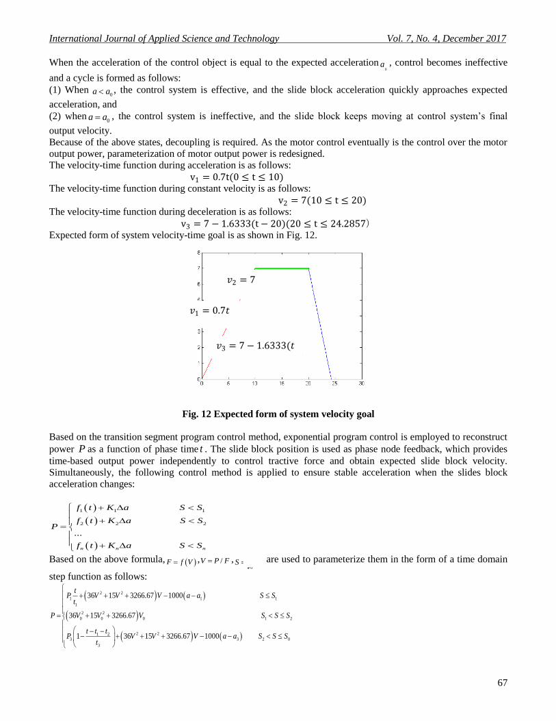
The velocity-time function during acceleration is as follows:

v1 = 0.7t(0 ≤ t ≤ 10) The velocity-time function during constant velocity is as follows:

v2 = 7(10 ≤ t ≤ 20) The velocity-time function during deceleration is as follows:

v3 = 7 − 1.6333(t − 20)(20 ≤ t ≤ 24.2857） Expected form of system velocity-time goal is as shown in Fig. 12.

Fig. 12 Expected form of system velocity goal

Based on the transition segment program control method, exponential program control is employed to reconstruct

power P as a function of phase time t . The slide block position is used as phase node feedback, which provides

time-based output power independently to control tractive force and obtain expected slide block velocity.

Simultaneously, the following control method is applied to ensure stable acceleration when the slides block

acceleration changes:

1 1 1

2 2 2

...

n n n

f t K a S S

f t K a S SP

f t K a S S

Based on the above formula, F f V , /V P F ,0

t

S Vdt are used to parameterize them in the form of a time domain

step function as follows:

2 2

1 1 1

1

2 2

0 0 0 1 2

2 21 23 3 2 0

3

36 15 3266.67 1000

36 15 3266.67

1 36 15 3266.67 1000

tP V V V a a S S

t

P V V V S S S

t t tP V V V a a S S S

t

t

𝑣1 = 0.7𝑡

𝑣2 = 7

𝑣3 = 7 − 1.6333(𝑡

− 20)

V

t


68

where: 1P is the maximum power in a rising velocity segment,

1 1 0P maV ; 3P is the maximum power in a declining

velocity segment, 3 3 0P ma V ;

0V is the expected stable velocity, 7 /m s ;1 2 3, ,t t t are the times of motion in the rising

velocity segment, the stable velocity segment and the declining velocity segment, respectively;1 2 3, ,a a a are

accelerations in the rising velocity segment, the stable velocity segment and the declining velocity segment,

respectively; and 1 2 3 0, , ,S S S S are displacement lengths in rising velocity segment, stable velocity segment,

declining velocity segment and overall stroke. The applied control rule requires no end-to-end control variable

feedback, has simple structure and is easy to implement in hardware. Under the above three velocity states, the

slide block has 11 variables, which are1 2 3 1 2 3 0 1 2 3 0, , , , , , , , , ,t t t a a a V S S S S . However, the following are known variables:

0 1 2 27 0.7 0 12 120V a a t S ，，，， (9)

The constraint relations among the variables are as follows:

2 2

1 0 1 1 1 1 2 0 2 3 0 1 2 3 3 3 3 0 3

1/ 2 / /

2t V a S a t S V t S S S S a S t a V t ，，，，， (10)

The formulae show that when five variables are obtained, the other seven variables can be calculated. Therefore,

to change the control rule, only five variables must be changed. From among them, five variables need

confirmation, i.e.,0 1 0 2 2, , , ,V a S t a .

Based on formula (9), expected displacement and expected velocity variation in the range of allowed

displacement values are obtained.

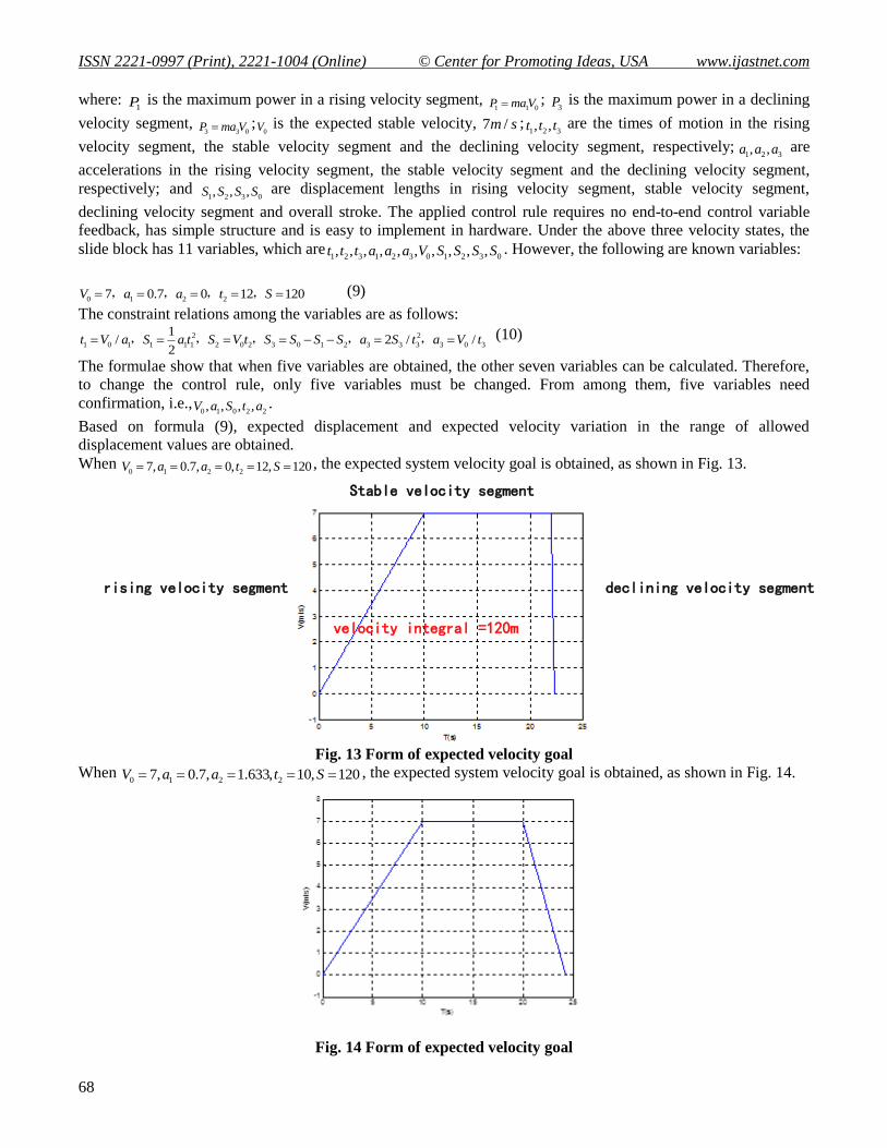
When 0 1 2 27, 0.7, 0, 12, 120V a a t S , the expected system velocity goal is obtained, as shown in Fig. 13.

Fig. 13 Form of expected velocity goal

When 0 1 2 27, 0.7, 1.633, 10, 120V a a t S , the expected system velocity goal is obtained, as shown in Fig. 14.

Fig. 14 Form of expected velocity goal

Stable velocity segment

declining velocity segment

velocity integral =120m

rising velocity segment


69

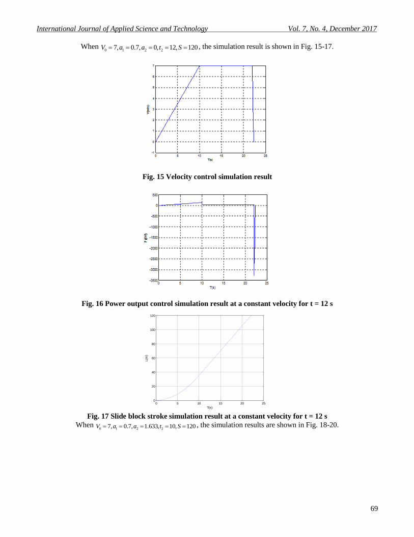
When 0 1 2 27, 0.7, 0, 12, 120V a a t S , the simulation result is shown in Fig. 15-17.


Fig. 16 Power output control simulation result at a constant velocity for t = 12 s

Fig. 17 Slide block stroke simulation result at a constant velocity for t = 12 s

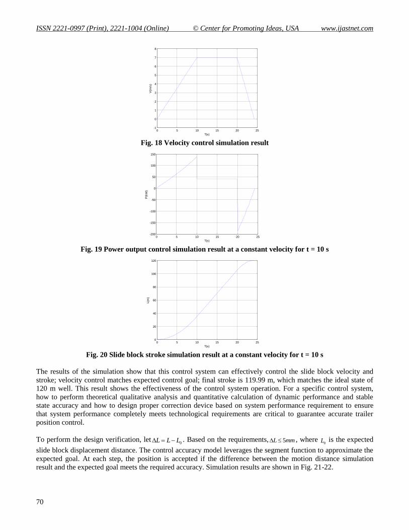
When 0 1 2 27, 0.7, 1.633, 10, 120V a a t S , the simulation results are shown in Fig. 18-20.

0 5 10 15 20 250

20

40

60

80

100

120

T(s)

L(m

)


70


Fig. 19 Power output control simulation result at a constant velocity for t = 10 s

Fig. 20 Slide block stroke simulation result at a constant velocity for t = 10 s

The results of the simulation show that this control system can effectively control the slide block velocity and

stroke; velocity control matches expected control goal; final stroke is 119.99 m, which matches the ideal state of

120 m well. This result shows the effectiveness of the control system operation. For a specific control system,

how to perform theoretical qualitative analysis and quantitative calculation of dynamic performance and stable

state accuracy and how to design proper correction device based on system performance requirement to ensure

that system performance completely meets technological requirements are critical to guarantee accurate trailer

position control.

To perform the design verification, let0L L L . Based on the requirements, 5L mm , where

0L is the expected

slide block displacement distance. The control accuracy model leverages the segment function to approximate the

expected goal. At each step, the position is accepted if the difference between the motion distance simulation

result and the expected goal meets the required accuracy. Simulation results are shown in Fig. 21-22.

0 5 10 15 20 25-1

0

1

2

3

4

5

6

7

8

T(s)

V(m

/s)

0 5 10 15 20 25-200

-150

-100

-50

0

50

100

150

T(s)

P(k

W)

0 5 10 15 20 250

20

40

60

80

100

120

T(s)

L(m

)


71

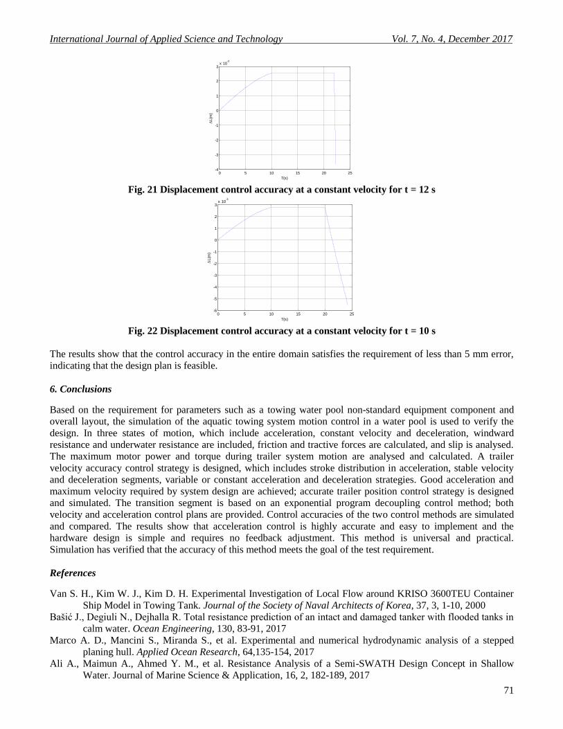
Fig. 21 Displacement control accuracy at a constant velocity for t = 12 s

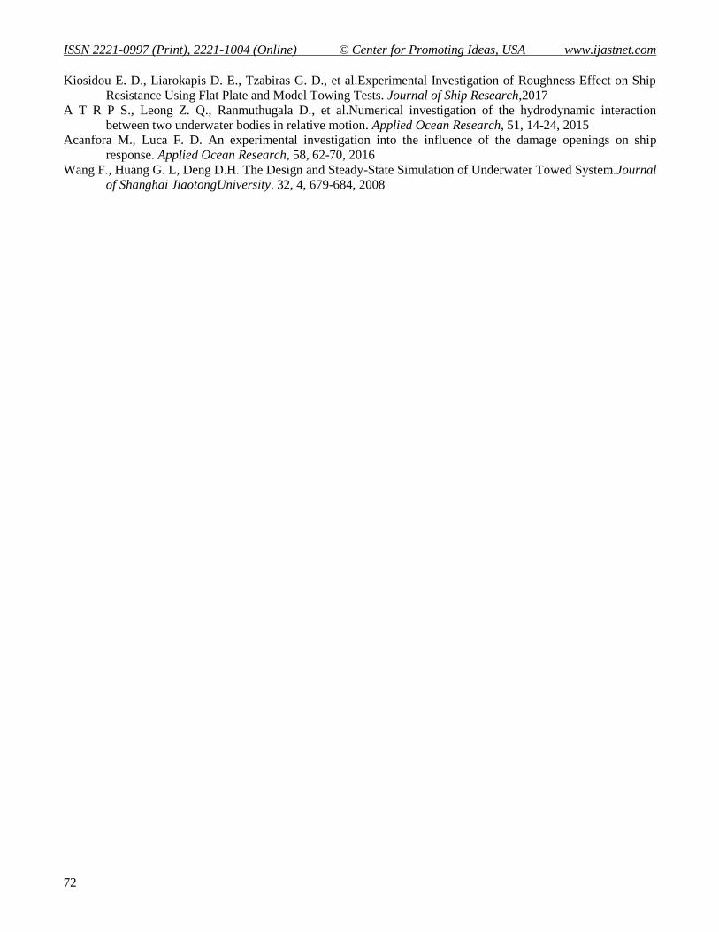
Fig. 22 Displacement control accuracy at a constant velocity for t = 10 s

The results show that the control accuracy in the entire domain satisfies the requirement of less than 5 mm error,

indicating that the design plan is feasible.

6. Conclusions

Based on the requirement for parameters such as a towing water pool non-standard equipment component and

overall layout, the simulation of the aquatic towing system motion control in a water pool is used to verify the

design. In three states of motion, which include acceleration, constant velocity and deceleration, windward

resistance and underwater resistance are included, friction and tractive forces are calculated, and slip is analysed.

The maximum motor power and torque during trailer system motion are analysed and calculated. A trailer

velocity accuracy control strategy is designed, which includes stroke distribution in acceleration, stable velocity

and deceleration segments, variable or constant acceleration and deceleration strategies. Good acceleration and

maximum velocity required by system design are achieved; accurate trailer position control strategy is designed

and simulated. The transition segment is based on an exponential program decoupling control method; both

velocity and acceleration control plans are provided. Control accuracies of the two control methods are simulated

and compared. The results show that acceleration control is highly accurate and easy to implement and the

hardware design is simple and requires no feedback adjustment. This method is universal and practical.

Simulation has verified that the accuracy of this method meets the goal of the test requirement.

References

Van S. H., Kim W. J., Kim D. H. Experimental Investigation of Local Flow around KRISO 3600TEU Container

Ship Model in Towing Tank. Journal of the Society of Naval Architects of Korea, 37, 3, 1-10, 2000

Bašić J., Degiuli N., Dejhalla R. Total resistance prediction of an intact and damaged tanker with flooded tanks in

calm water. Ocean Engineering, 130, 83-91, 2017

Marco A. D., Mancini S., Miranda S., et al. Experimental and numerical hydrodynamic analysis of a stepped

planing hull. Applied Ocean Research, 64,135-154, 2017

Ali A., Maimun A., Ahmed Y. M., et al. Resistance Analysis of a Semi-SWATH Design Concept in Shallow

Water. Journal of Marine Science & Application, 16, 2, 182-189, 2017

0 5 10 15 20 25-4

-3

-2

-1

0

1

2

3x 10

-3

T(s)

L(m

)

0 5 10 15 20 25-6

-5

-4

-3

-2

-1

0

1

2

3x 10

-3

T(s)

L(m

)


72

Kiosidou E. D., Liarokapis D. E., Tzabiras G. D., et al.Experimental Investigation of Roughness Effect on Ship

Resistance Using Flat Plate and Model Towing Tests. Journal of Ship Research,2017

A T R P S., Leong Z. Q., Ranmuthugala D., et al.Numerical investigation of the hydrodynamic interaction

between two underwater bodies in relative motion. Applied Ocean Research, 51, 14-24, 2015

Acanfora M., Luca F. D. An experimental investigation into the influence of the damage openings on ship

response. Applied Ocean Research, 58, 62-70, 2016

Wang F., Huang G. L, Deng D.H. The Design and Steady-State Simulation of Underwater Towed System.Journal

of Shanghai JiaotongUniversity. 32, 4, 679-684, 2008

motion control and simulation of a towing tank … · trailer of towing tank is the basic equipment...

Documents