mosfet and set co-simulation - smdpii-vlsi:special ... · mosfet and set co-simulation chaitanya...
TRANSCRIPT
MOSFET and SET co-simulation
Chaitanya Sathe
II MEDepartment of Electrical communication Engineering
Indian Institute of ScienceBangalore
India
December 7, 2006
Outline
I Brief introduction of Monte Carlo Method
I Monte Carlo Simulator for Single-Electron Tunnel Devices (SIMON)
I Master Equation
I Macro-modeling of SET
I CAD framework for SET-MOS Co-simulation
I Case study
Chaitanya, IISc MOSFET and SET co-simulation 2/28

What are Monte Carlo Methods ?
I Can be viewed as a branch of experimental mathematics in whichone uses random numbers to conduct experiments.
I Typically the experiments are done on a computer using anywherefrom hundreds to billions of random numbers
I Very roughly speaking, we can categorize Monte Carlo experimentsinto the following two broad classes
I Direct simulation of a naturally random systemI Addition of artificial randomness to a system,followed by simulation
of the new system
Chaitanya, IISc MOSFET and SET co-simulation 3/28

Estimating π using Monte Carlo Method
+1
+1
−1
− 1
π =40
13= 3.079
If we use 10000 points we get π = 3.1728
Chaitanya, IISc MOSFET and SET co-simulation 4/28
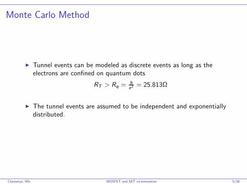
Monte Carlo Method
I Tunnel events can be modeled as discrete events as long as theelectrons are confined on quantum dots
RT > Rq = he2 = 25.813Ω
I The tunnel events are assumed to be independent and exponentiallydistributed.
Chaitanya, IISc MOSFET and SET co-simulation 5/28

Flow Chart of Monte Carlo Method
PSfrag replacements
Parse circuit file
Build capacitance matrix and prepare
for computation of node potential and free energy
for each possible tunnel event:
compute free energy change
compute tunnel rate
compute duration to next tunnel event
Choose event with smallest duration and
update charges accordingly
time limit ?
accuracy limit ?
event limit?
yes
no
stop
Chaitanya, IISc MOSFET and SET co-simulation 6/28
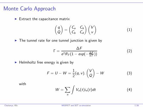
Monte Carlo Approach
I Extract the capacitance matrix
(
q
Q
)
=
(
Ca Cb
Cb Cd
) (
V
v
)
(1)
I The tunnel rate for one tunnel junction is given by
Γ =∆F
e2RT (1 − exp(−∆FkT
))(2)
I Helmholtz free energy is given by
F = U − W =1
2(q, v).
(
V
Q
)
− W (3)
with
W =∑
n
∫
Vn(t)in(t)dt (4)
Chaitanya, IISc MOSFET and SET co-simulation 7/28
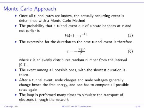
Monte Carlo ApproachI Once all tunnel rates are known, the actually occurring event is
determined with a Monte Carlo MethodI The probability that a tunnel event out of a state happens at τ and
not earlier isP0(τ) = e−Γτ (5)
I The expression for the duration to the next tunnel event is therefore
τ = −log r
Γ(6)
where r is an evenly distributes random number from the interval[0,1].
I The event among all possible ones, with the shortest duration istaken.
I After a tunnel event, node charges and node voltages generallychange hence the free energy, and one has to compute all possiblerates again.
I The loop is performed many times to simulate the transport ofelectrons through the network
Chaitanya, IISc MOSFET and SET co-simulation 8/28
Master Equation method
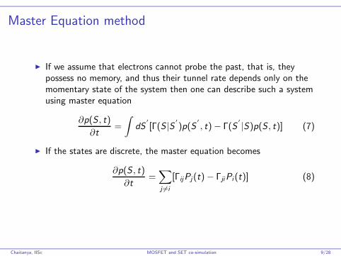
I If we assume that electrons cannot probe the past, that is, theypossess no memory, and thus their tunnel rate depends only on themomentary state of the system then one can describe such a systemusing master equation
∂p(S , t)
∂t=
∫
dS′
[Γ(S |S′
)p(S′
, t) − Γ(S′
|S)p(S , t)] (7)
I If the states are discrete, the master equation becomes
∂p(S , t)
∂t=
∑
j 6=i
[ΓijPj (t) − ΓjiPi (t)] (8)
Chaitanya, IISc MOSFET and SET co-simulation 9/28

Master Equation methodI The master equation is a description of the underlying Markov
Process of electrons tunneling from island to island.
I A state is a specific charge distribution , each node or quantum dotis occupied by a certain number of electrons.
I The master equation method for the simulation of single-electroncircuits tries to solve these equations.
PSfrag replacements1
2
3
4
5
Figure: State transition diagram
Chaitanya, IISc MOSFET and SET co-simulation 10/28
Master Equation method
I Although the Master equation method gives theoretically accurateresults, it has many other impracticability’s that limit its accuracyand usability.
I The starting point of the ME is the set of all relevant states a circuitwill occupy during operation.
I There is no way to filter out these states a priori from an arbitrarycircuit.
I One way is to include many more states than would be relevant,which results in extremely long simulation times and sometimes badnumerical stability.
I Another way out is to use an adaptive algorithm which alleviates thisproblem.
Chaitanya, IISc MOSFET and SET co-simulation 11/28
Advantages AND Disadvantages of A Monte Carlo
Approach
I It gives better transient and dynamic characteristics of SET circuitsbecause it models the underlying microscopic physics in a very directmanner.
I It is not required to find the relevant states before one can start withthe actual simulation as in the case of a master equation.
I It is easy to trade accuracy with simulation time, and therefore canquickly achieve approximate results of very large circuits.
I One major disadvantage of the Monte Carlo method is simulatingco-tunneling events
Chaitanya, IISc MOSFET and SET co-simulation 12/28
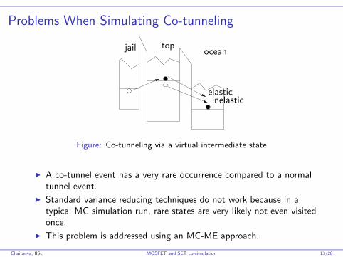
Problems When Simulating Co-tunneling
PSfrag replacements
jail topocean
elasticinelastic
Figure: Co-tunneling via a virtual intermediate state
I A co-tunnel event has a very rare occurrence compared to a normaltunnel event.
I Standard variance reducing techniques do not work because in atypical MC simulation run, rare states are very likely not even visitedonce.
I This problem is addressed using an MC-ME approach.
Chaitanya, IISc MOSFET and SET co-simulation 13/28
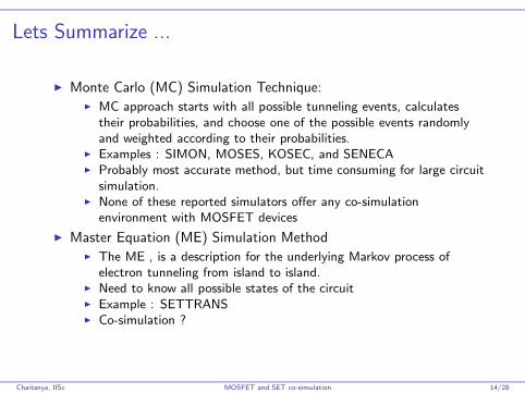
Lets Summarize ...
I Monte Carlo (MC) Simulation Technique:I MC approach starts with all possible tunneling events, calculates
their probabilities, and choose one of the possible events randomly
and weighted according to their probabilities.I Examples : SIMON, MOSES, KOSEC, and SENECAI Probably most accurate method, but time consuming for large circuit
simulation.I None of these reported simulators offer any co-simulation
environment with MOSFET devices
I Master Equation (ME) Simulation MethodI The ME , is a description for the underlying Markov process of
electron tunneling from island to island.I Need to know all possible states of the circuitI Example : SETTRANSI Co-simulation ?
Chaitanya, IISc MOSFET and SET co-simulation 14/28
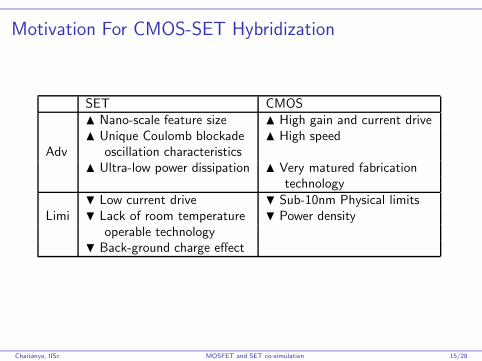
Motivation For CMOS-SET Hybridization
SET CMOSN Nano-scale feature size N High gain and current driveN Unique Coulomb blockade N High speed
Adv oscillation characteristicsN Ultra-low power dissipation N Very matured fabrication
technologyH Low current drive H Sub-10nm Physical limits
Limi H Lack of room temperature H Power densityoperable technology
H Back-ground charge effect
Chaitanya, IISc MOSFET and SET co-simulation 15/28
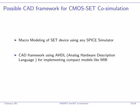
Possible CAD framework for CMOS-SET Co-simulation
I Macro Modeling of SET device using any SPICE Simulator
I CAD framework using AHDL (Analog Hardware DescriptionLanguage ) for implementing compact models like MIB
Chaitanya, IISc MOSFET and SET co-simulation 16/28

Macro Modeling of SET deviceI The following assumptions are made in compact simulators like
SPICE to simulate the characteristics of any given circuit topology.I Once the model parameters of a device are determined from the
device simulator or other modeling tools, it can be used in the whole
circuit.I The I-V characteristics of the device are affected by neighboring
transistors only through the changes of the terminal voltages of
those transistors, the interaction between adjacent devices is usually
neglected.
I The second assumption in the case of SET circuits may not ingeneral be valid.
I When the size of interconnection between the SET devices is largeenough, the interconnection acts like a reservoir rather than aCoulomb island.
I In that case, the Coulomb islands of SET’s become isolated by theinterconnection and the interaction among neighboring SET’s is notsignificant.
I CL ≥ 6.25Cj for the compact model to be valid
Chaitanya, IISc MOSFET and SET co-simulation 17/28
Macro Modeling of SET device
−
+
+
−
PSfrag replacements
gate
drain
source
gate drain
source
RG
R1R2 R3
D1 D2
vpvp
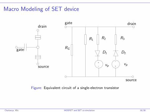
Figure: Equivalent circuit of a single-electron transistor
Chaitanya, IISc MOSFET and SET co-simulation 18/28

Macro Modeling of SET device
I Symmetric features of the drain-source current-voltage (Ids − Vds)characteristics are incorporated with two branches consisting of thecombinations of resistors, diodes and voltagesources(R2/D1/VPandR3/D2/VP).
I The directions of D1 and VP are opposite with those of D3 and V3
to have adequate current flow in both positive and negativedrain-source bias.
I The charging energy, periodically changing as a function of the gatebias, is included in R1, R2, and R3 where the cosine of the gate biasis used
R1(VG ) = CR1 + CR2cos(CF1VG ) (9)
R2(VG ) = R3(VG ) =CVp
CI2 −2CVp
R1(VG )
(10)
Chaitanya, IISc MOSFET and SET co-simulation 19/28
Macro Modeling of SET device
I The parameters, CF1, CVp , CI2, CR1, andCR2 are used to fit the I-Vcharacteristics at various gate biases.
I Since the SET characteristics of SET’s strongly depend on T, themacromodel parameters are a function of T.
I SPICE macromodeling of single-electron transistors can be used forefficient circuit simulations, these macromodels produce simulationresults with reasonable accuracy and are faster than Monte Carlosimulations.
I This technique is non-physical (empirical) in nature.
I The technique is also not scalable
Chaitanya, IISc MOSFET and SET co-simulation 20/28

CMOS-SET CO-SIMULATION using VERLOG-A
I Verilog-A Hardware Description Language (HDL) is a behaviorallanguage for analog and mixed signal systems.
I Verlog-A enables to compactly model the device behaviour
PSfrag replacements Verilog-A
SET model
VerilogA
Compiler
C file
C-compiler
.so fileSMARTSPICE
RUN
SOURCE
SPICE
NETLIST
Chaitanya, IISc MOSFET and SET co-simulation 21/28

CMOS-SET CO-SIMULATION using VERLOG-A
VerilogA SET Module Standard spice Netlistmodule set (drain,gate1,gate2,source); .verilog ”set.va” // includes the SET module
inout drain,gate1,gate2,source;
electrical drain,gate1,gate2,source; M1 2 2 4 4 MOD1 L1=0.5U W=0.8U
M2 3 2 4 4 MOD1 L=0.5U W=0.8U
//Default value of the model parameters .....................
parameter real CTS = 1e-18,CTD = 1e-18 .....................
parameter real CG = 2e-18,CG2 =0
parameter real RTD = 1e6,RTS = 1e6 VDD 1 0 5
parameter real XI=0 VSS 4 0 5
.....................
.....................
analog YVLGmyset 1 3 6 7 0 set CG1=2e-18
begin // Instantiate SET
//MIB subroutine
I(drain,source) =.... .dc VIN 0.0 0.04 0.008
end .end
endmodule
Chaitanya, IISc MOSFET and SET co-simulation 22/28
Case Study: Modeling Analysis of Noise Margin in SET
Logic
VOH
VOL
VIH
VIL
"0"
"1"
NMH
NML
GateOutput
GateInput
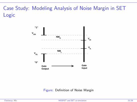
Figure: Definition of Noise Margin
Chaitanya, IISc MOSFET and SET co-simulation 23/28
Case Study: Modeling Analysis of Noise Margin in SET
Logic
−20 −15 −10 −5 0 5 10 15 20−20
−15
−10
−5
0
5
10
15
20
VOUT
VIN
VOH
VOL
VIL
VIH
A
B
C
D
VMAX
VMIN
region 1
region 2
region 3
VSS
VDD
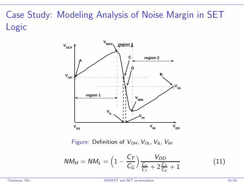
Figure: Definition of VOH , VOL, VIL, VIH
NMH = NML =(
1 −CT
CG
) VDD
CG
CT+ 2CT
CG+ 1
(11)
Chaitanya, IISc MOSFET and SET co-simulation 24/28

Case Study: Modeling Analysis of Noise Margin in SET
Logic
10−2
10−1
100
101
102
−0.5
0
0.5
1
1.5
2
2.5
3
Temperature in K
NM
H (
NM
L )
in m
V
CG
:CT=3C
G:C
T=5
CG
:CT=7
β>40
T=11.5K
Figure: Effect of Temperature on Noise Margin
Chaitanya, IISc MOSFET and SET co-simulation 25/28
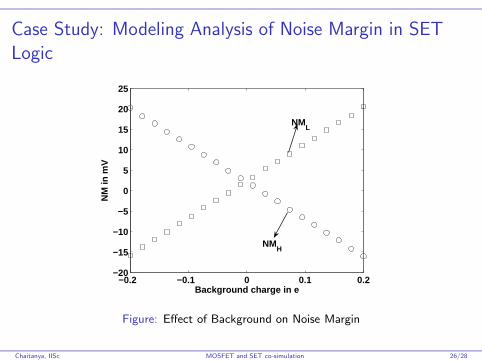
Case Study: Modeling Analysis of Noise Margin in SET
Logic
−0.2 −0.1 0 0.1 0.2−20
−15
−10
−5
0
5
10
15
20
25
Background charge in e
NM
in m
V
NMH
NML
Figure: Effect of Background on Noise Margin
Chaitanya, IISc MOSFET and SET co-simulation 26/28
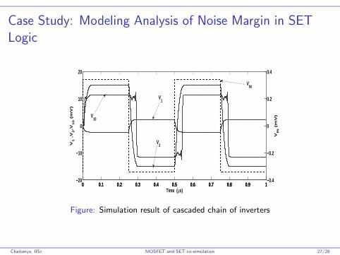
Case Study: Modeling Analysis of Noise Margin in SET
Logic
0 0.1 0.2 0.3 0.4 0.5 0.6 0.7 0.8 0.9 1−20
−10
0
10
20V
1 ,V
2,V
10 (
mV
)
0 0.1 0.2 0.3 0.4 0.5 0.6 0.7 0.8 0.9 1−0.4
−0.2
0
0.2
0.4
Time (µs)
VIN
(m
V)
VIN
V1
V2
V10
Figure: Simulation result of cascaded chain of inverters
Chaitanya, IISc MOSFET and SET co-simulation 27/28

References
I Lectures on Monte Carlo Methods. Neal Madras, AmericanMathematical Society
I SIMON - A Simulator for Single-Electron Tunnel Devices andCircuits. Christoph Wasshuber et al, IEEE Transactions ofComputer-Aided Design of Integrated Circuits and Systems VOL.16,NO. 9,SEP 1997
I Computational Single - Electronics. Christoph Wasshuber, Springer
I Macromodeling of single electron transistors for efficient circuitsimulation. Y.S.Yu et al ,IEEE Trans.Elec.Dev vol46 no8
I Hybrid CMOS Single Electron Transistor Device and Circuit Design.Santanu Mahapatra et al , Artech House Publication 2006
I Modeling and analysis of noise Margin in SET Logic. Chaitanya etal, International Conference on VLSI Design 2007
Chaitanya, IISc MOSFET and SET co-simulation 28/28