morris thesis final - ut m

To the Graduate Council:

I am submitting herewith a thesis written by Daniel H. Morris entitled “Price Relationships among Wholesale Ethanol, Wholesale Gasoline, and Retail Gasoline: A Study on Asymmetrical Pricing and Lag Relationships.” I have examined the electronic copy of this thesis for form and content and recommend that it be accepted in partial fulfillment of the requirements for the degree of Master of Science, with a major in Agriculture and Natural Resources.

Dr. Scott Parrott Major Professor

We have read this thesis and recommend its acceptance:

Dr. Joey Mehlhorn

Dr. Rachna Tewari

Accepted for the Council

Dr. Victoria S. Seng Associate Vice Chancellor for Academic Affairs and Dean of Graduate Studies

(Original signatures are on file with official student records)

Price Relationships among Wholesale Ethanol, Wholesale Gasoline, and Retail Gasoline:

A Study on Asymmetrical Pricing and Lag Relationships

A Thesis Presented for

the Master of Science Degree

The University of Tennessee at Martin

Daniel H. Morris

November 2013

ii Acknowledgements

I would like to thank Dr. Scott Parrott for his tireless efforts to make sure this research

came together. It would have been impossible for me to complete this work without his guidance

and expertise in regard to the statistical analysis of this research. I am truly indebted to him for

all his input and support. I would also like to thank Dr. Barbara Darroch for helping with the

formation of this thesis. I am also thankful for the assistance provided by Oil Price Information

Services for clarifying some of the questions we had in regard to the price data. I would also like

to express my sincere gratitude to Dr. Joey Mehlhorn for his guidance and friendship during my

time as both an undergraduate and graduate student. I have benefited greatly from the entire

agricultural faculty and have been blessed to know each and everyone of you. Finally, I would

like to thank my incredible wife, Heather, for her continued support and understanding during

my time spent in the graduate program at UTM.

iii Abstract

The volatile relationship between commodity prices and fuel prices has been a hot topic

in the agricultural sector over the past few years due to the sporadic market conditions that have

resulted in record high commodity prices. Drought like conditions that have persisted over the

course of 2011 and especially 2012 led to record high grain prices across the nation. During this

time frame, gasoline prices remained volatile as well, but did not follow the same trend as corn

futures prices. This is somewhat puzzling as the price of gasoline consists of the underlying price

of crude oil and the price of the ethanol that is part of the blended fuel. This posed the questions,

what is the direct price relationship between gasoline prices and ethanol prices and how are price

changes passed through? In order to answer these questions, we also had to look at the price

relationship at the wholesale and retail levels to ensure that price changes were passed through

the distribution chain. We discovered the underlying price of gasoline is not dependent upon

current commodity prices as the grain purchased for processing is purchased at a different time.

That changed the focus of our research to concentrate on the price relationship between

wholesale gasoline prices and retail gasoline. The objective of our research was to determine the

level of asymmetry between wholesale gasoline, which consists of pure gasoline and pure

ethanol, and retail gasoline.

The primary focus for our research was the Little Rock, Arkansas market as this was the

closest geographical region that had the complete price data for pure gasoline, pure ethanol, and

retail gasoline. The data used in this research was obtained from Oil Price Information Service

(OPIS) and consisted of the daily price of each fuel component variable for the Little Rock

market. All of the price data was compiled and analyzed using SAS to generate all of the

statistical analysis that is laid forth in this thesis. The price data was first analyzed using the

iv Pearson Coefficient Correlation test to determine the correlation between gasoline and ethanol

prices. After the correlation between the variables was confirmed, the data needed to be

converted into an empirical model to test for the presence of asymmetry between the variables.

The Houck Procedure was utilized in order to transform the data set into a more malleable form

that would be better suited for the asymmetry model. The next step in the analysis was to

perform a Granger Causality test in order to figure the lag length between the wholesale level

and the retail level. The PDLREG procedure was then utilized within SAS to simultaneously

perform GLS regressions to account for any auto-correlated errors and to establish parameter

estimates for the data set. The PDLREG procedure forced the data set to lie on the 5th degree

polynomial distributed lag due to the results of the Pearson Correlation Coefficient test. After

finalizing the results of the PDLREG procedure, pairwise comparisons were used to test for the

presence of asymmetry amongst the data set, which was the final step in the data analysis.

The results of our research indicated the existence of asymmetry between wholesale and

retail gasoline prices. Our model showed that price changes are passed through directly from the

wholesale level to the retail level with asymmetry being more prevalent under the presence of

fuel price increases. The model also revealed the lack of asymmetry between ethanol and retail

gasoline prices. Our research concluded there was no difference between rising and falling

ethanol prices in regard to changes in retail gasoline prices. Further research needs to be

conducted in order to draw extensive conclusions about the price relationship of gasoline and

ethanol.

v Table of Contents

Chapter 1: Introduction ................................................................................................................... 1

Chapter 2: Literature Review ........................................................................................................... 3

Ethanol Industry Analysis .................................................................................................... 3

Asymmetrical Price Relationships ....................................................................................... 6

Purpose of Study ................................................................................................................. 8

Chapter 3: Method ......................................................................................................................... 10

Source ............................................................................................................................... 10

Methods ............................................................................................................................ 12

Chapter 4: Results and Discussion ................................................................................................. 14

Chapter 5: Conclusion .................................................................................................................... 22

List of References ........................................................................................................................... 24

Appendix ........................................................................................................................................ 27

Vita …… .......................................................................................................................................... 36

vi List of Figures

Figure A.1. All Price Data ................................................................................................................ 28

Figure A.2. Corn Futures and Fuel Prices ....................................................................................... 29

Figure A.3. Fuel Prices in Little Rock, Arkansas .............................................................................. 30

Figure A.4. WTI Index 3/1/2011 to 9/30/2012 .............................................................................. 31

Figure A.5. Corn Futures 3/1/2011 to 9/30/2012 .......................................................................... 31

vii List of Tables

Table A.1. Descriptive Statistics and Lagged Price Correlations of the Wholesale and Retail

Price Series.............................................................................................................32

Table A.2. Granger Causality Test for Regular Gasoline Little Rock up to 11 Lags ........32

Table A.3. Granger Causality Test for Wholesale Regular Gasoline Little Rock up to

11 Lags ...................................................................................................................33

Table A.4. Granger Causality Test for Pure Ethanol up to 11 Lags ..................................33

Table A.5. PDLREG Procedure Results ............................................................................34

Table A.6: Pairwise Comparison Results ..........................................................................35

1 Chapter 1: Introduction

This study will focus on the effect of changes in the prices of pure ethanol and

wholesale gasoline on the price of retail gasoline. The relationship between gasoline and

ethanol is important to the agricultural community in that both commodities are vitally

important to agricultural production. The price of gasoline and ethanol can be extremely

volatile. Market swings can negatively impact the profitability of producers. It is

imperative to have a better understanding of the relationship between ethanol and

gasoline to be able to explain the impact that one has on the other. As a better

understanding of the relationship between ethanol and gasoline prices is developed,

American agribusinesses will be better equipped to reduce their risk associated with any

major swings in the price of one of the two variables. This study will concentrate on the

relationship between ethanol and gasoline because there appears to be a lack of research

on this topic. Ethanol is a vital part of America’s agricultural sector as approximately one

third of the corn crop is processed into ethanol to be blended with gasoline as a fuel

additive. The existing government mandate that ethanol be blended with gasoline

provides support to the ethanol industry within the United States. For the near term, it

appears the federal mandate will not be suspended and ethanol production will continue

into the foreseeable future. It is necessary to better understand the price relationship

between ethanol and gasoline so the price direction for both gasoline and ethanol can be

gauged. This thesis attempts to determine the impact changes in wholesale gasoline and

pure ethanol have on retail gasoline prices. It was elected for this study to test for the

presence of asymmetry between wholesale prices and retail prices in order to see just how

price changes are passed through from one stage to the next.

2 The focus of this study will be the impact of the price relationship between

ethanol and gasoline within the Little Rock, Arkansas market. This market was chosen

due to the complete fuel price data that was readily available for this particular market.

This study will examine whether the price relationship between the fuels at the wholesale

level and at the retail level are symmetric or asymmetric in nature. This will be answered

by determining how changes in wholesale gasoline prices are passed through to the retail

level. Further statistical analysis was conducted in order to evaluate the lag response in

the prices of pure ethanol, wholesale gasoline, and retail gasoline.

3 Chapter 2: Literature Review

This literature review consists of two parts to establish some background relevant

to this study. The first part of the literature review will discuss ethanol and its inherent

relationship to gasoline. This was done to provide the reader further insight as to why

fluctuations in grain prices and ethanol prices are directly linked to the final price of

gasoline. The second portion of the literature review will focus on relevant examples of

asymmetrical price studies.

Ethanol Industry Analysis:

Ethanol (ethyl alcohol) is an alcohol-based fuel that is created by fermenting grain

and separating the alcohol from the coarse grains, typically by means of distillation.

Ethanol has been used to power machinery for years and has numerous properties that

make it a suitable fuel source for internal combustion engines, which in turn makes it a

viable fuel source for automobiles (Frazier, 2009). Ethanol is also a reliable fuel additive

that can be blended with gasoline to curb the total amount of crude oil needed to meet the

energy demands of the United States. Recent research estimates half of the gasoline sold

in the United States contains up to 10% ethanol (E10) (Frazier, 2009). Ethanol helps

boost the octane of gasoline by 2 to 3 points in an E10 blend (Frazier, 2009). When

blended with gasoline, ethanol acts as a reformulating chemical agent and adds an

additional oxygen atom to the emissions during the combustion process. This reduces the

total amount of pollutants created from the fuel exhaust of a gasoline-powered vehicle,

making ethanol-gas blends a more environmentally friendly fuel source than pure

gasoline.

4 World ethanol production in 2006 was approximately 13.5 billion gallons with the

United States being the world’s largest producer of ethanol (Onuki et al., 2008). The

average ethanol processing facility produces approximately 65 million gallons of ethanol

each year (First Research, 2013). The global biofuel market generates $83 billion in

revenue on an annual basis with the United States, China, the European Union, and Brazil

being the largest ethanol producers (First Research, 2013). As of June 2013, the U.S. was

the world’s largest ethanol producer with an annual production of 14 billion gallons (First

Research, 2013). In the United States, corn can represent up to 60% of ethanol production

costs as it is the main raw material needed for ethanol production. In the United States,

most ethanol is produced from corn by means of dry milling, which produces 2.8 gallons

of ethanol from 1 bushel of corn. Ethanol can also be processed by means of wet milling;

however, this processing method produces only 2.7 gallons of ethanol per 1 bushel of

corn (Onuki et al., 2008). As corn is the key ingredient in U.S. ethanol production,

ethanol is attractive to the agricultural community both as a means for securing a more

reliable fuel supply and for increasing the demand for agricultural products (Frazier,

2009). As such, ethanol is a fuel source that can be sourced domestically and helps to

reduce the overall amount of petroleum used in the United States. Petroleum imports used

in American gasoline production declined from 60% in 2005 to 45% in 2011 due to the

ethanol blended in gasoline and to more petroleum being produced domestically (First

Research, 2013). However, lower fuel economy from ethanol-gasoline blends and the

high production costs could prevent ethanol from becoming a long term solution for the

energy needs of the United States.

5 Ethanol does have disadvantages when utilized as a blending agent in gasoline.

Ethanol, as an E10 blend, is known to reduce the fuel economy of passenger vehicles by

an estimated 2.2% (Frazier, 2009). This is partially due to ethanol having lower energy

content when compared to gasoline. Ethanol is also more corrosive than pure gasoline

and has been known to cause degradation of rubber and plastic components of engines.

The corrosive nature of ethanol can cause rubber fuel lines and gaskets to fail, resulting in

down time and costly repairs. Due to its alcohol content, ethanol is a very strong solvent

that can help remove build up and deposits in fuel systems. However, this can result in

clogged fuel filters which can reduce the overall performance of an engine. Ethanol also

attracts moisture if it sits idle for extended periods of time. This aspect of ethanol can be

detrimental to engines on smaller pieces of equipment that remain idle for months at a

time such as lawn mowers and other similar outdoor power equipment.

The negative traits of ethanol have created some consumer resentment to the

inclusion of ethanol in gasoline. However, a government mandate of an E10 fuel blend

keeps the demand for ethanol high, as it requires gasoline producers to blend ethanol with

gasoline. The Energy Independence & Security Act of 2007 requires that 36 billion

gallons of renewable fuel be blended with gasoline by 2022. This legislation was passed

as a response to rising oil prices. Periods of high oil prices encourage investment in

alternative fuel sources. The Energy Independence & Security Act gives American

companies an incentive to increase research and development capital expenditures in

regard for ethanol processing techniques and production methods. Ethanol demand is

driven by federal legislation and regulations and as such the ethanol market is a

government mandated market.

6 Asymmetrical Price Relationships:

Asymmetrical pricing examines whether prices rise and fall at the same rate.

Based on a review of the literature, it is apparent that most asymmetrical price studies are

centered on the relationship between crude oil and fuel prices. For example, studies

conducted by Bacon (1990), Karrenbrock (1991), Borenstein, Cameron, and Gilbert

(1992) all focused on some aspect of the asymmetrical relationship between crude oil and

gasoline. That being said, the following section of this paper will focus on additional

research that pertains to the asymmetric price relationship between crude oil and gasoline

to serve as an example of testing for asymmetry. Again, the focus of this study is on

asymmetric pricing between ethanol and gasoline at both the wholesale and retail levels.

Research suggests there is indeed an asymmetric price relationship between crude

oil and gasoline prices. The evidence of such a relationship is most apparent when crude

oil prices are rising. Typically, gasoline prices rise as a direct response to higher crude oil

prices. This relationship is not as clear when crude oil prices are declining. This

observation is often referred to as the “rocket feather effect” in that the price at the pump

increases at a very fast pace in response to higher crude oil prices while prices decline at

a much slower rate as the cost of oil per barrel decreases. Bacon (1990) indicated there

was an asymmetrical price relationship between crude oil and gasoline prices in the

United Kingdom. Further studies conducted by Karrenbrock (1991) emphasized there

tends to be a stronger relationship between crude oil and gasoline prices under the

conditions of rising prices. Borenstein, Cameron, and Gilbert (1992) suggested gasoline

prices do in fact respond asymmetrically to rising crude oil prices. They indicated there is

strong and ubiquitous evidence of asymmetry between crude oil and gasoline prices.

7 Borenstein et al. used bivariate error correction models that tested for asymmetry in price

movements in gasoline and crude oil at various stages of the production and distribution

process. Research conducted by Balke, Brown, and Yucel (1998) suggested the

relationship between crude oil and gasoline could be seen all the way from the refinery to

the pump.

Other research is not so clear on the evidence of price asymmetry in price and

output. Tinsley and Krieger (1997) concluded that negative asymmetry was more

apparent in a manufacturing setting and positive asymmetry was seen more when

producer pricing occurs. This could be applied to the relationship between crude oil and

gasoline as refiners act as manufacturers of gasoline as it is a byproduct of the refining

process. The refiners price gasoline, and other fuels, to vendors, which is an example of

producer pricing. Tinsley and Krieger (1997) further concluded that asymmetry in pricing

may possibly be attributed to asymmetric movements in output and the sign of price

responses were due to the utilization rate of the output, which in this case is fuel.

Asymmetric pricing is more than an “econometric curiosity” as it provides details in

regard to variations in average response time of prices within a certain industry (Tinsley

and Krieger, 1997). Asymmetric pricing models provide insight into the relationship

between related variables in order to help economists determine how a price change in

one variable will impact the other. This research will focus on testing for the presence of

asymmetry between two distinct price relationships found in the energy sector.

The current study will examine the changes in prices on a daily basis to determine

whether the relationship between wholesale and retail levels is symmetrical or

asymmetrical. Researchers have completed numerous studies that tested for the symmetry

8 between crude oil, fuel, and the overall price of energy. An example of this type of

research can be found in a study conducted by Huntingdon (1998), who found that energy

prices respond symmetrically to petroleum product prices. Huntingdon (1998) also

discovered the majority of asymmetry in the economy’s reaction to crude oil price

fluctuations occurred within the energy industry, and more specifically, within oil

markets. Huntingdon’s research was an attempt to answer the question as to whether

changes in oil prices have a direct impact on macroeconomic activities or not.

Huntingdon’s work utilized vector autoregressive techniques to try to explain the impact

oil price shocks have on the overall economy. Acquah & Ofosuhene (2013) indicated the

“dynamics in price transmission has attracted considerable research interest among

agricultural economists; of particular interest is the issue of asymmetric price

relationship.” Acquah and Ofosuhene (2013) looked for a model that would provide a

better fit when testing for complete asymmetrical price relationships. This particular

study noted various statistical methods used to test for asymmetrical pricing with most

emphasis being placed on which asymmetric price model is the most reliable. Acquah

and Ofosuhene (2013) concluded that the accuracy of the asymmetric price model was

dependent upon the size of the data set and the overall complexity of the model.

Purpose of Study

This study focused on addressing the relationship between ethanol and gasoline

prices, both of which are crucial to the agricultural sector. Additionally, this study

focused on the relationship between the three variables over the course of 18 months

spanning from 3/1/2011 to 9/31/2012. The prices for ethanol were extremely volatile

during these 18 months, given the drastic price fluctuations in corn futures. During this

9 time, the price of corn varied from a low of $5.52 per bushel to a high of $8.31. Most of

the volatility that occurred during this time was due to the 2012 drought, which

contributed to the increase in corn prices. The increase in corn prices was the main cause

of the fluctuations in ethanol prices from 3/1/2011 to 9/30/2012. This in turn affected

gasoline prices due to the ethanol blend that is mandated by the federal government. As

gasoline is comprised of refined crude oil and an ethanol blend, any change in the price

of its components (i.e. crude oil and corn) will have a direct impact on its price. A goal of

this research was to show how a change in any of these variables directly or indirectly

affects the others. Also, as the data is from the same time frame, any relationship between

variables was deemed to be contemporaneous in nature.

Another factor to consider when determining changes in prices is the elasticity of

the product. The elasticity of demand for the product will directly impact the utilization

rate of the output. The elasticity of demand for fuel is relatively stable as fuel is needed to

power automobiles, transport goods, and generate electricity. The demand for ethanol is

relatively stable as well due to the government mandated ethanol blend with gasoline.

10 Chapter 3: Methods

Source:

To analyze the relationships between crude oil, gasoline, and ethanol prices, the

daily price data for the time frame from 3/1/2011 to 9/30/2012 was used. The crude oil

price used in the analysis was the daily spot price for West Texas Intermediate (WTI)

crude oil. The WTI crude oil daily spot price was retrieved from United States Energy

Information Administration. The daily retail price for gasoline was for regular unleaded

gasoline at local retail service stations located in Little Rock, Arkansas. The daily

wholesale price used in this study was based on research conducted by the Oil Price

Information Service (OPIS) and represents the average daily price for regular unleaded

gasoline and 10% conventional ethanol blend within the designated market from

3/1/2011 through 9/30/2012. OPIS collects the data from gasoline retailers within certain

markets (i.e. cities) in a daily survey. The data is averaged to determine a daily price for

each city surveyed. The price data used in this study contained 580 observations for each

variable.

Certain edits were made to the WTI historical price data and the fuel prices that

were utilized for this study. Gasoline prices are calculated on a daily basis at both the

wholesale and retail level. However, grain futures and ethanol data are not compiled on a

daily basis. Therefore, the grain futures and ethanol price data were adjusted to reflect a

daily price to match up with the wholesale and retail fuel data for both gasoline and

diesel. The grain futures used in the study represent the futures price of corn at the

closing of trade on the Chicago Mercantile Exchange (CME). Grain futures are traded on

the CME Monday through Friday as the CME does not trade on weekends or on national

11 holidays. Therefore, the closing price from the previous day was used for the price of

corn futures for every day the CME is not open for trade (i.e. Sundays, Saturdays, and

national holidays). Ethanol prices are not reported on Sundays so the closing price for

ethanol on Saturdays was substituted as the price of ethanol on all Sundays in our study.

This was done in order to have a daily price for every variable contained in this study:

crude oil, gasoline, diesel, ethanol, and corn futures.

This study included a test for correlation between the daily futures price of corn

and ethanol prices with the intention of testing for asymmetry between the two variables.

It was anticipated that the tests would result in a direct correlation between the futures

price of corn and ethanol since ethanol is derived from corn. It was determined that a

comparison between the daily price of corn and the daily price of pure ethanol could not

be made as the corn that was used in the ethanol production process was priced in a

different time period. Ethanol producers purchase corn using various futures prices to

lock in a favorable price. This is typically done months in advance so ethanol producers

can determine their costs of production. Therefore, the price of corn futures used to

purchase corn for processing is based on a different futures price than the daily futures

price traded on the CME. Comparing the daily futures price of corn to the price of pure

ethanol, was not an accurate comparison and the results from the correlation tests for the

price relationship between the futures price of corn and pure ethanol have been excluded

from this study.

Transportation costs are sometimes included in price transmission models.

However, transportation costs were excluded from this study. The retailers that provided

the retail gasoline price data buy gasoline from terminals and wholesalers in multiple

12 locations with the distance between each location being fixed. Transportation costs are

viewed as a fixed cost and are part of the fuel price paid by retailers to wholesalers.

Therefore, the transportation costs of fuel are already included in the price data used in

this study.

Methods:

The price data was analyzed using SAS to perform all of the statistical analysis.

The price data consisted of the daily price for wholesale gasoline, the daily price for pure

ethanol, and the daily price for retail gasoline (i.e. E10 blend). The price data was first

analyzed using the Pearson Coefficient Correlation test for the existence of any

correlation between gasoline and ethanol prices.

The Pearson Correlation Coefficient equation is as follows:

where r = the Pearson Correlation Coefficient between wholesale and retail

gasoline prices. After confirming the correlation between gasoline and ethanol prices, the

data was transformed into a slightly different format before being tested for the existence

of asymmetry between the variables. The Houck Procedure was used to transform the

structure of the data set so it would be better suited for the asymmetry model. The Houck

procedure was performed to test for nonreversibilities within the data set. The next step

was to conduct a Granger Causality test to determine the causality between wholesale

prices and retail prices. The next process was to use the PDLREG procedure within SAS

to perform GLS regressions to account for any auto-correlated errors and to create

13 parameter estimates for the model. The equation for the PDLREG procedure is as

follows:

Where, xt is the regressor with a disributed lag effect, zt is a simple covariate, and ut is an

error term (SAS, 2010). The PDLREG procedure specifies the degree of the polynomial

lag, which for this thesis was to the 5th degree. After completing the results of the

PDLREG procedure, pair wise comparisons were used to test for asymmetry within the

data set. The pair wise comparison between rising and falling prices was the final step in

the data analysis.

14 Chapter 4: Results and Discussion

Note that all the tables and figures can be found in the appendix section. The test

for asymmetry begins with electing both upstream variables and downstream variables.

The upstream variable typically represents the price of a main input or a price at a higher

market level than retail. The upstream prices used in this study are the price of wholesale

ethanol and wholesale gasoline. A downstream variable tends to consist of an output

price or a price at a lower market level such as the retail price of a product. For this study,

the downstream variable is the retail price of gasoline. The test for asymmetry examines

whether retail prices react the same to rising or falling wholesale gasoline and ethanol

prices.

Pearson Correlation Coefficients were calculated to test for price asymmetry

between pure ethanol, wholesale gasoline, and retail gasoline. The coefficient can range

from -1 to +1 and indicates the degree of linear dependence between the variables. The

closer the coefficient is to either -1 or +1, then the stronger the relationship between the

variable being measured. The Pearson Correlation Coefficients were calculated to

determine the length of a lag in price responses between each pair of variables. The

lagged correlation between wholesale gasoline and retail gasoline prices peaks at day 5

(Table A.1). This indicates that the effect of a price change has the greatest impact 5 days

later at the retail level and then begins to decline. The evidence of a lagged correlation

between wholesale and retail gasoline prices is the first step in the test for asymmetry

between the two variables. The Pearson Coefficient Correlation test revealed the lack of a

lag relationship between ethanol and gasoline prices. The underlying price of retail

gasoline does not appear to be strongly correlated with the wholesale price of gasoline.

15 This was likely caused by the lack of a direct relationship between the two variables.

Unlike crude oil and gasoline, ethanol does not have a direct link to gasoline as ethanol is

not a major component of gasoline. The underlying price of ethanol is mainly driven by

the cost of the corn that is used in the production process. The lack of an inherent price

relationship between ethanol and gasoline prevents the existence of a lag relationship

between the two variables.

The second part of initial testing was to test the lag response in prices changes of

conventional clear gasoline and ethanol, which are the two components of wholesale

gasoline. This test helps to determine when the price of either pure gasoline or pure

ethanol changed; the result of the change is passed along to the price of retail gasoline.

The model assumes the following:

Prg = f (Rising/Falling Pcg; Rising/Falling Ppe)

Where Prg is the retail price of gasoline is the result of the function of rising/falling price

of conventional gasoline (Pcg) and the rising/falling price of pure ethanol (Ppe). A Pearson

Correlation Coefficients test was performed in order to determine the length of a lag in

price responses between conventional gasoline paired with pure ethanol and retail

gasoline. The results of our Pearson Correlation Coefficient test indicated there is a

strong positive correlation between the price of wholesale gasoline and the price of retail

gasoline. After it was determined the variables were correlated, the next step was to test

for symmetry or the lack thereof (i.e. asymmetry) among the variables.

The next step involved testing for model specification using a Granger Causality

test. The Granger Causality test can determine if one variable is useful for forecasting

another variable. The test uses a series of F-tests to determine whether the lagged data for

16 a variable Y provides any statistically significant information about variable X in the

presence of lagged variable X. A time series X is useful in determining futures values of

Y if it can be proven by means of t-tests and F-tests that lagged values of X offer

statistically significant information in regard to future values of Y. If the empirical results

of the Granger Causality test are significant, then the direction of causation can be

determined (i.e. change in X causes change in Y). If wholesale gasoline prices are a

function of retail gasoline prices, then the inclusion of wholesale gasoline prices as an

explanatory variable could possibly create simultaneity bias (Kesselring, 2009).

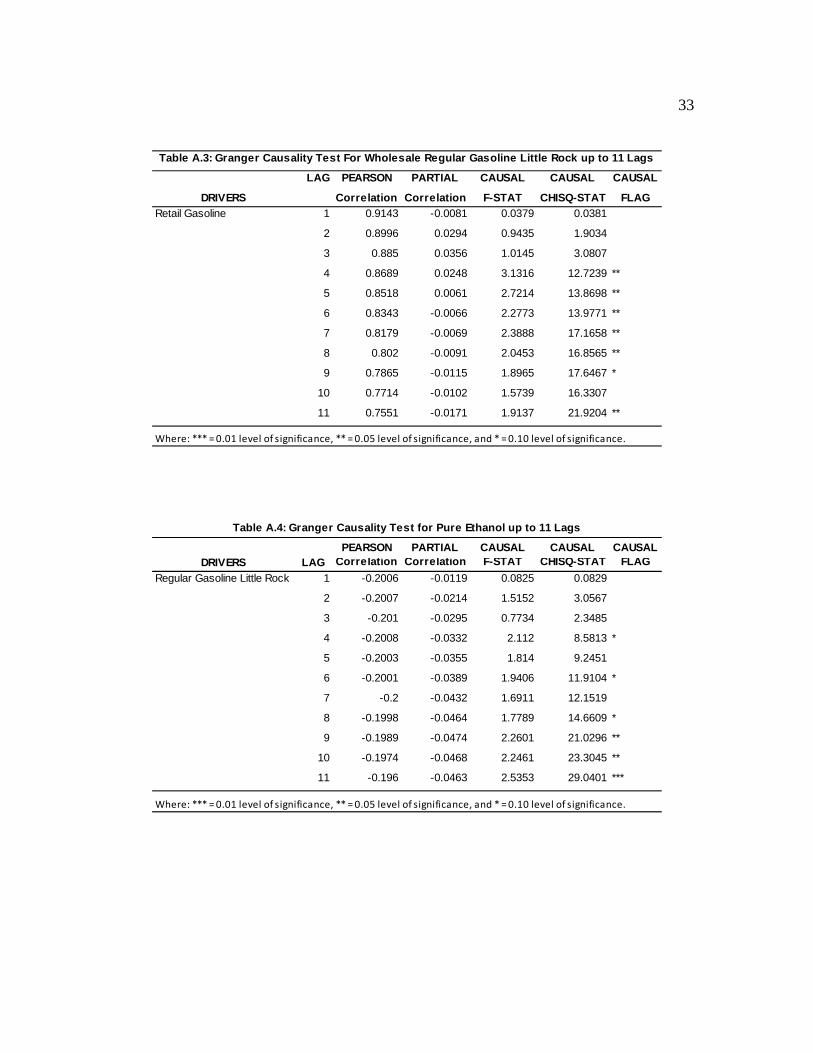
Granger causality tests were conducted on the two variables and ethanol in this

study to ensure the causality is unidirectional, running from wholesale gasoline prices to

retail gasoline prices. According to the Granger Causality test, there was overwhelming

evidence indicating that when the retail price of gasoline is the dependent variable and

wholesale prices are the independent variable, the causality flows from the wholesale

price to the retail price. This is illustrated by the F-stat for all lags of wholesale gasoline

being statistically significant in regard to retail gasoline (Table A.2). However, when

wholesale prices are the dependent variable and retail price of gasoline is the independent

variable, the causality between the variables appears to be sporadic. The results of the

Granger Causality test led to the conclusion that the causality flows from the wholesale

level (i.e. wholesale gasoline and pure ethanol) to the retail level (i.e. retail gasoline).

However, the causality does not flow from the retail price of gasoline back to the

wholesale level. Therefore, the direction of the causality flows from the wholesale level

directly to the retail level. This is expected, as the retail price of gasoline is the

17 downstream variable whose price is dependent upon the price of wholesale gasoline,

which is the upstream variable

The data set was then converted into a better format to test for asymmetry. The

Houck procedure was used to alter the price data into a better form to conduct

asymmetrcial testing. The Houck procedure tests for nonreversibilities in a particular data

set. Nonreversibilities are most commonly expressed in terms of asymmetrical changes

from a previous position in time, which makes the initial observation vital to the test.

The Houck procedure was utilized in this study to estimate the nonreversible functions of

our price model. The Houck procedure is an operationally clear method of determining

the nonreversible functions within a data set and commonly used among agricultural

economists as it has been applied across a variety of commodities (Parrott et al., 2001).

The namesake of the procedure, J. P. Houck, has noted that the methodology does have

its limitations. The procedure consumes two degrees of freedom to account for the added

price variable and the loss of explanatory power from the original observation (Houck,

1977). The procedure also can intensify intercorrelations among variables. However, if

the variable that is segmented is highly correlated with another variable, the segmentation

may lower the intercorrelation issue (Houck, 1977). For the purposes of this study, the

Houck procedure was deemed to be a reliable method to test for nonreversible functions.

The procedure does not produce actual statistical test results as it serves only to prepare

the data for symmetry analysis. For this study, a new dependent variable for retail prices

was created to represent the current period’s price less the initial starting point price. The

independent variable in this study was wholesale gasoline and was separated into two

different fields, rising wholesale prices and falling wholesale prices.

18 The next step in the statistical analysis was to perform a Generalized Least

Squares statistical analysis to find the appropriate lag lengths for rising and falling prices.

The lag length of 8 for rising prices and the lag length of 11 for falling prices were

determined by means of Generalized Least Squares (GLS) regressions. The lag length of

8 days for rising prices tell us that a price increase only takes 8 days to pass through

while a price decrease takes 11 days to pass through based on the lag length of 11 days

for falling prices. Only the significant lag lengths were retained.

After that, the next step was to perform a polynomial distribution lag regression

(PDLREG) procedure to estimate the lag distribution. This particular procedure was

because of the observed existence of a lag relationship between wholesale and retail

prices. The PDLREG procedure is a statistical test that can be performed using the

statistical analysis software SAS. The PDLREG procedure results in a regression analysis

complete with polynomial distributed lags. This particular procedure establishes

parameters estimates for the data set with estimates of the lag distribution. For our study,

we used the 5th degree polynomial because of the correlation relationships observed. The

PDLREG procedure forced the rising and falling wholesale prices to lie on a 5th degree

polynomial. The PDLREG procedure results also indicated the lack of a polynomial lag

relationship between pure ethanol prices and retail gasoline prices. The parameter

estimates for rising prices revealed that the t-values for Rising(0), Rising(3), Rising(4),

Rising(5), Rising(6), and Rising(8) were all significant (p < 0.10; Table A.5). The

parameter estimate for Falling(1), Falling(2), Falling(3), Falling(6), Falling(7), Falling(8),

Falling(10), and Falling(11) were deemed to be highly significant (p < 0.10). These

estimates are significantly different from 0 and allowed for statistical inferences to be

19 made about the data set. The PDLREG procedure results also indicated there was no lag

amongst ethanol prices. This was determined by the GLS regression portion of the

PDLREG procedure (p > 0.01; Table A.5).

The next step was to test for the presence of asymmetry by imposing restrictions

on the independent variables. Pairwise comparisons can be made if both the estimates of

the lag distribution for rising and falling prices are statistically significant from 0 at the

same lag period. For example, a pairwise comparison cannot be made between Rise(0)

and Fall(0) as the variable Fall(0) is not statistically significant (Table A.5). However,

Rise(0) is statistically significant, which leads to the inference that a portion of an

increase in wholesale gasoline prices was passed along with the remainder of the price

increase that is passed through the lag. In the event of a price decrease, the current price

is not transmitted instantaneously because the falling price variable was not significant.

Research conducted by Borenstein et al. (1992) support the findings that changes in

wholesale prices are not passed through immediately to the retail level. Their research

indicated that changes in wholesale gasoline prices are not felt at the retail level until 7 to

14 days later. Pairwise comparisons between the estimates of the lag distribution for

Rise(4) & Fall(4) and Rise(5) & Fall(5) prices could not be made (p > 0.10); Table A.5).

A pairwise comparison could also not be made for Rise(1) and Fall(1) prices as Rise(1)

was not statistically significant even though Fall(1) was statistically significant (p <

0.01). This scenario was the same for Rise(2) and Fall(2), Rise(7) and Fall(7), Rise(10)

and Fall (10), as well as Rise(11) and Fall(11) due to the falling price variable being

statistically significant while the rising price variable was not statistically significant

20 (Table A.5). A pair wise comparison could not be made for Rise(9) and Fall(9) prices as

neither the rising nor the falling price variable was statistically significant.

A pair wise comparison could be completed for the Rise(3) & Fall(3), Rise(6) &

Fall(6), and Rise(8) & Fall(8) prices as both the rising and falling price variables were

found to be statistically significant. The following pair wise comparisons test for the

existence of an asymmetrical price relationship by means of t-tests for the restriction. If

the corresponding p-value of the t-test were found to be statistically significant, then

inferences could be made about how price changes are passed through. The pair wise

comparisons for the Rise(3) & Fall(3), Rise(6) & Fall(6), and Rise(8) & Fall(8) prices

were not significant (p > 0.10; Table A.5). The pair wise comparison between rising and

falling ethanol prices was also not statistically significant (p = 0.1332), which indicated

there was no difference in pricing behavior.

The overall asymmetry model dictated only the first 8 days can be evaluated as

this was the end point of the rising lag. The results of this asymmetry test indicated a

significant difference in the way retailers transfer price increases to the customer versus

price decreases. The overall test for asymmetry was positive and statistically significant,

implying that when comparing the first 8 days after a change in wholesale gasoline

prices, the price increases are transferred quicker than wholesale gasoline price decreases.

This was illustrated by the significant overall asymmetry test (p > 0.0001). Also, the 11th

day of the price decrease lag was highly significant (p < 0.0001) with an 11th day lag

falling price parameter of 0.2859 (Table A.5). The asymmetry test results for ethanol

revealed that there was no difference in rising versus falling ethanol prices with respect to

retail gasoline. The asymmetry model indicated there was no difference in how price

21 changes of ethanol are passed on the retail level based on the pairwise comparison for

rising and falling ethanol prices (p > 0.01; Table A.6). Both increases and decreases in

ethanol prices are treated in the same manner and are directly passed on by retailers. This

was not the case with wholesale gasoline price changes as the Rise(0) and Fall(0)

wholesale price increases were treated differently by retailers. The difference in the

treatment of ethanol price changes versus wholesale price changes by retailers may be

explained due to the composition of gasoline. For this study, retail gasoline consisted of

90% wholesale gasoline and 10% pure ethanol. Therefore, a change in wholesale gasoline

prices would have a larger impact on the retail price of gasoline due to the inherent

relationship between the two. Ethanol price changes seem to have been absorbed in the

transfer from the wholesale level to the retail level as it only represented a small portion

of the retail gasoline blend.

22 Chapter 5: Conclusion

The results of our study clearly indicate retail gasoline prices respond with a lag

to wholesale gasoline price changes with there being no evidence of asymmetry with

respect to retail gasoline and ethanol. For asymmetry testing, only the first 8 days could

be looked at as this is where the rising price lag concluded. However, the lagged response

can be estimated to a level where it is possible to recognize the asymmetric responses to

wholesale gasoline price changes. Our test results indicated retail gasoline prices respond

faster to increases in wholesale gasoline than to decreases. This was proven by the test for

asymmetry being both positive and significant when comparing the first 8 days following

a change in wholesale gasoline prices. Thus, the level of asymmetry appears to be most

prevalent between the responses of retail gasoline prices to increases in wholesale

gasoline price changes. This was expected as the retail price of gasoline is dependent

upon the wholesale price of gasoline.

Based on the results of the model, it can be concluded there was a level of price

asymmetry between wholesale gasoline and retail gasoline in the Little Rock, Arkansas

market between the dates of 3/1/2011 to 9/30/2012. The findings of this research indicate

the presence of asymmetry between wholesale and retail gasoline prices was less severe

than previous research. Research conducted by Borenstein et al (1992) concluded the

existence of asymmetry between wholesale and retail gasoline prices was more severe

than the result of this thesis. Borenstein et al. (1992) concluded that asymmetry was

clearly visible between the wholesale and retail levels. However, research conducted by

Balke et al. (1998) concurred with the research findings of this thesis. Balke et al. (1998)

found the existence of asymmetry between wholesale and retail gasoline prices to be

23 minor and was present in only a few cases. The lack of severity of asymmetry in the

model could be attributed to use of daily price data for this thesis. However, both the

studies performed by Borestein et al. (1992) and Balke et al. (1998) used yearly price

data, but the findings of each study varied greatly from one another.

The asymmetrical relationship between retail gasoline and pure ethanol was more

difficult to determine due to the lack of a polynomial lag relationship between retail

gasoline prices and ethanol prices. However, it appears the level of asymmetry between

the two variables was more sporadic. The explanation for this phenomenon may be due to

the fact that ethanol makes up a small percentage of the retail gasoline blend and

represents a smaller part of the retail gasoline price as a result. Further research needs to

be conducted to determine the asymmetrical relationship between pure ethanol and retail

gasoline prices over a longer period of time.

24

List of References

25 References:

Acquah, H.D. and Ofosuhene, P. (2013). The Role of Model Complexity and the

Performance of the Selection Criteria in Asymmetric Price Transmission Models. Journal of Economics and Behavioral Studies, 5(3), 157-163.

Bacon, R. W. (1990). Rockets & Feathers: The Asymmetric Speed of Adjustment of UK

Retail Gasoline Prices to Cost Changes. Oxford Institute for Energy Studies. Balke, N.S., Brown, S.P.A., and Yucel, M.K. (1998). Crude Oil and Gasoline Prices: An

Asymmetric Relationship?. Federal Reserve Bank of Dallas Economic Review, First Quarter 1998, 2-11.

Borenstein, S., Cameron, A.C., and Gilbert, R. (1992). Do Gasoline Prices Respond

Asymmetrically to Crude Oil Price Changes?. National Bureau of Economic Research, August, NPER Paper No. 4138.

First Research. (2013). Industry Profile: Biofuel Manufacturing. Austin, TX. First

Research Staff. Frazier, R. S. (2009). Ethanol Gasoline Blends-Problems or Benefits for Customers?.

Energy Engineering, 106(1), 62-70. Houck, J.P. (1977). An Approach to Specifying and Estimating Nonreversible Functions.

American Journal of Agricultural Economics, 59(3), 570-572. Huntingdon, H.G. (1998). Crude Oil Prices and U.S. Economic Performance: Where

Does the Asymmetry Reside?. The Energy Journal, 19(41), 107-132. Karrenbrock, J. D. (1991). The Behavior of Retail Gasoline Prices: Symmetric or Not?.

Federal Reserve Bank of St. Louis Review, July/August, 19-29. Kesselring, R.G. and Bremmer, D.S. (2009). Presentation from 51st Annual Meeting of

the Western Social Science Association: Gasoline and Crude Oil: Evidence of Asymmetric Price Changes during 2008?. Albuquerque, NM.

Onuki, S., Koziel, J.A., van Leeuwen, J. H., Jenks, W.S., Grewell, D., and Cai, L. (2008).

Ethanol production, purification, and analysis techniques: a review.Presentation from 2008 ASABE Annual International Meeting: Providence, RI.

Parrott, S.D., Eastwood, D. B., and Brooker, J.R. (2001). Testing for Symmetry in Price

Transmission: An Extension of the Shiller Lag Structure with an Application to Fresh Tomatoes. Journal of Agribusiness, 19(1), 35-49.

SAS Institute Inc. 2010. SAS/ETS® 9.22 User’s Guide. Cary, NC: SAS Institute Inc.

26 Tinsley, P.A. and Krieger, R. (1997). Asymmetric Adjustments of Price and Output.

Economic Inquiry, July, 35(3), 631-652.

27

Appendix

Figures and Tables

28

Fig

ure

A.1

: 3/1

/201

1 to

9/3

0/20

12 D

aily

Cor

n F

utur

es, D

aily

WT

I C

rude

Oil

Pri

ces,

and

Dai

ly F

uel

Pri

ce D

ata

for

the

Lit

tle

Roc

k M

arke

t

29

Fig

ure

A.2

: Cor

n F

utur

es P

rice

and

Dai

ly F

uel P

rice

s be

twee

n 3/

1/20

11 a

nd 9

/30/

2012

30

Fig

ure

A.3

: Fue

l Pri

ces

in L

ittl

e R

ock

31 Figure A.4: WTI Index

Figure A.5: Corn Futures

32

Table A.1: Pearson Correlation Coefficients between Wholesale and Retail Gas Prices in the Little Rock, Arkansas Market; March 2011 to September 2012:

(A)Item Retail Wholesale EthanolMean ($) 3.41 2.98 2.75Range ($) 2.99-3.84 2.55-3.47 2.29-3.19Coeff. Of Variation 0.06 0.07 9.19

(B)

Item t t · 1 t · 2 t · 3 t · 4 t · 5 t · 6 t · 7 t · 8 t · 9

Retail Seriest 0.91598 0.92251 0.93323 0.93714 0.93907 0.93774 0.93471 0.92990 0.92375 0.91666

Wholesale Price Periods:Lagged Price Correlations

Table A.1: Descriptive Statistics and Lagged Price Correlations of the Wholesale and Retail Price SeriesDescriptive Statistics

PEARSON PARTIAL CAUSAL CAUSAL CAUSALCorrelation Correlation F-STAT CHISQ-STAT FLAG

Wholesale Gasoline 1 0.9421 0.5169 210.4097 211.5037 ***

2 0.9508 0.5919 59.2371 119.5045 ***

3 0.9563 0.6286 39.6567 120.4234 ***

4 0.96 0.6537 30.0371 122.0422 ***

5 0.961 0.6588 23.4729 119.6336 ***

6 0.9587 0.6452 19.0042 116.6398 ***

7 0.9542 0.6267 16.0802 115.5496 ***

8 0.9477 0.6054 14.3194 118.0138 ***

9 0.9398 0.5851 12.5802 117.0567 ***

10 0.9309 0.5652 11.329 117.5458 ***

11 0.9214 0.5474 10.254 117.4521 ***

Pure Ethanol 1 -0.202 -0.0308 0.5511 0.554

2 -0.2033 -0.0419 1.1936 2.4081

3 -0.205 -0.0531 1.2688 3.8529

4 -0.2071 -0.064 0.9391 3.8155

5 -0.2093 -0.0737 0.969 4.9386

6 -0.2117 -0.0832 1.1426 7.0129

7 -0.214 -0.091 1.0811 7.7686

8 -0.216 -0.0975 1.0514 8.6653

9 -0.2181 -0.104 0.902 8.3925

10 -0.2206 -0.1111 1.0108 10.488

11 -0.2235 -0.1186 0.9577 10.9697

Where: *** = 0.01 level of significance, ** = 0.05 level of significance, and * = 0.10 level of significance.

Table A.2: Granger Causality Test For Regular Gasoline Little Rock up to 11 Lags

DRIVERS LAG

33

PEARSON PARTIAL CAUSAL CAUSAL CAUSAL

Correlation Correlation F-STAT CHISQ-STAT FLAG

Retail Gasoline 1 0.9143 -0.0081 0.0379 0.0381

2 0.8996 0.0294 0.9435 1.9034

3 0.885 0.0356 1.0145 3.0807

4 0.8689 0.0248 3.1316 12.7239 **

5 0.8518 0.0061 2.7214 13.8698 **

6 0.8343 -0.0066 2.2773 13.9771 **

7 0.8179 -0.0069 2.3888 17.1658 **

8 0.802 -0.0091 2.0453 16.8565 **

9 0.7865 -0.0115 1.8965 17.6467 *

10 0.7714 -0.0102 1.5739 16.3307

11 0.7551 -0.0171 1.9137 21.9204 **

Table A.3: Granger Causality Test For Wholesale Regular Gasoline Little Rock up to 11 Lags

DRIVERS

LAG


PEARSON PARTIAL CAUSAL CAUSAL CAUSALCorrelation Correlation F-STAT CHISQ-STAT FLAG

Regular Gasoline Little Rock 1 -0.2006 -0.0119 0.0825 0.0829

2 -0.2007 -0.0214 1.5152 3.0567

3 -0.201 -0.0295 0.7734 2.3485

4 -0.2008 -0.0332 2.112 8.5813 *

5 -0.2003 -0.0355 1.814 9.2451

6 -0.2001 -0.0389 1.9406 11.9104 *

7 -0.2 -0.0432 1.6911 12.1519

8 -0.1998 -0.0464 1.7789 14.6609 *

9 -0.1989 -0.0474 2.2601 21.0296 **

10 -0.1974 -0.0468 2.2461 23.3045 **

11 -0.196 -0.0463 2.5353 29.0401 ***

Table A.4: Granger Causality Test for Pure Ethanol up to 11 Lags

DRIVERS LAG


34

Variable Estimate

Conventional_Clear_Reg_Rise(0) 0.1520**

Conventional_Clear_Reg_Rise(1) 0.0795



Conventional_Clear_Reg_Rise(4) 0.1476***

Conventional_Clear_Reg_Rise(5) 0.1495***




Variable Estimate

Conventional_Clear_Reg_Fall(0) 0.0444

Conventional_Clear_Reg_Fall(1) 0.1530***

Conventional_Clear_Reg_Fall(2) 0.1142***

Conventional_Clear_Reg_Fall(3) 0.0495**







Conventional_Clear_Reg_Fall(10) 0.0755*Conventional_Clear_Reg_Fall(11) 0.2859***

Variable Estimate

Pure Ethanol Average Rising Price 0.2880

Pure Ethanol Average Falling Price 0.0108

Table A.5: The PDLREG Procedure

Where: *** = 0.01 level of s igni ficance, ** = 0.05 level of

Where: *** = 0.01 level of s igni ficance, ** = 0.05 level of

s igni ficance, and * = 0.10 level of s igni ficance.

*Neither the ri s ing or fa l l ing ethanol price was found to

be s igni ficant.

Estimate of Lag Distribution

Estimate of Lag Distribution

35

Pairwise Comparison P‐value of T‐test

Rise(3) and Fall(3) 0.3458



Rising and Falling Ethanol Prices (0 or current period) 0.1332

Overall Asymmetry Test (all periods together) <0.0001

Table A.6: Pairwise Comparison Results

36 Vita

Daniel Hunter Morris was born on December 2, 1988 and raised in the small rural

community of Skullbone, Tennessee. He graduated from Bradford High School in 2007.

In May 2011, he graduated from the University of Tennessee at Martin with a B.S. in

Agribusiness. In August 2011, he began earning his Master’s degree in Agriculture and

Natural Resource Systems Management with a concentration in Agribusiness and Risk

Management. He and his wife, Heather, currently reside in Sikeston, Missouri. Daniel is

currently employed as a commercial loan officer for a national bank in Sikeston,

Missouri.

morris thesis final - ut m

Documents