morphological filtering for image enhancement...
TRANSCRIPT

P. Maragos & L. Pessoa: Chapter for The Image and Video Processing Handbook, Acad. Press. 1
MORPHOLOGICAL FILTERING FOR IMAGEENHANCEMENT AND DETECTION
Petros Maragos(1) and Lucio F. C. Pessoa(2)
(1) Dept. of Electrical & Computer Engineering, National Technical University of Athens,Zografou 15773, Athens, Greece.
(2) Motorola, Inc., 3501 Ed Bluestein Blvd., Austin, TX 78721, U.S.A.Email: [email protected], Lucio [email protected]
March 1, 1999
1 Introduction
The goals of image enhancement include the improvement of the visibility and perceptibility ofthe various regions into which an image can be partitioned and of the detectability of the imagefeatures inside these regions. These goals include tasks such as: cleaning the image from varioustypes of noise; enhancing the contrast among adjacent regions or features; simplifying the image viaselective smoothing or elimination of features at certain scales and retaining only features at certaindesirable scales. While traditional approaches for solving the above tasks have used mainly toolsof linear systems, there is a growing understanding that linear approaches are not well suitableor even fail to solve problems involving geometrical aspects of the image. Thus there is a needfor nonlinear approaches. A powerful nonlinear methodology that can successfully solve the aboveproblems is mathematical morphology.
Mathematical morphology is a set- and lattice-theoretic methodology for image analysis, whichaims at quantitatively describing the geometrical structure of image objects. It was initiated [17] inthe late 1960’s to analyze binary images from geological and biomedical data as well as to formalizeand extend earlier or parallel work [13, 12] on binary pattern recognition based on cellular automataand Boolean/threshold logic. In the late 1970’s it was extended to gray-level images [17]. In themid 1980’s it was brought to the mainstream of image/signal processing and related to othernonlinear filtering approaches [7, 8]. Finally, in the late 1980’s and 1990’s it was generalized toarbitrary lattices [18, 2]. The above evolution of ideas has formed what we call nowadays the fieldof morphological image processing, which is a broad and coherent collection of theoreticalconcepts, nonlinear filters, design methodologies, and applications systems. Its rich theoreticalframework, algorithmic efficiency, easy implementability on special hardware, and suitability formany shape-oriented problems have propelled its widespread usage and further advancement bymany academic and industry groups working on various problems in image processing, computervision, and pattern recognition.
2 P. Maragos & L. Pessoa: Chapter for The Image and Video Processing Handbook, Acad. Press.
This chapter provides a brief introduction to the application of morphological image processingto image enhancement and detection. There are several motivations for using morphological filtersfor such problems. First, it is of paramount importance to preserve, uncover, or detect the geometricstructure of image objects. Thus, morphological filters which are more suitable than linear filtersfor shape analysis, play a major role for geometry-based enhancement and detection. Further,they offer efficient solutions to other nonlinear tasks such as non-Gaussian noise suppression. Thistask can also be accomplished (with similar performance) by a closely related class of nonlinearsystems, the median, rank and stack filters, which also outperform linear filters in non-Gaussiannoise suppression. Finally, the elementary morphological operators1 are the building blocks forlarge classes of nonlinear image processing systems, which include rank and stack filters.
2 Morphological Image Operators
2.1 Morphological Filters for Binary Images
Given a sampled2 binary image signal f [x] with values 1 for the image object and 0 for the back-ground, typical image transformations involving a moving window set W = {y1, y2, ..., yn} of nsample indexes would be
ψb(f)[x] = b(f [x− y1], ..., f [x− yn]) (1)
where b(v1, ..., vn) is a Boolean function of n variables. The mapping f �→ ψb(f) is called a Booleanfilter. By varying the Boolean function b, a large variety of Boolean filters can be obtained. Forexample, choosing a Boolean AND for b would shrink the input image object, whereas a BooleanOR would expand it. Numerous other Boolean filters are possible, since there are 22n
possibleBoolean functions of n variables. The main applications of such Boolean image operations havebeen in biomedical image processing, character recognition, object detection, and general 2D shapeanalysis [13, 12].
Among the important concepts offered by mathematical morphology was to use sets to representbinary images and set operations to represent binary image transformations. Specifically, given abinary image, let the object be represented by the set X and its background by the set complementXc. The Boolean OR transformation of X by a (window) set B is equivalent to the Minkowski setaddition ⊕, also called dilation, of X by B:
X⊕B ≡ {x+ y : x ∈ X, y ∈ B} =⋃
y∈B
X+y (2)
where X+y ≡ {x + y : x ∈ X} is the translation of X along the vector y. Likewise, if Br ≡ {x :−x ∈ B} is the reflection of B with respect to the origin, the Boolean AND transformation of Xby Br is equivalent to the Minkowski set subtraction �, also called erosion, of X by B:
X�B ≡ {x : B+x⊆X} =⋂
y∈B
X−y (3)
1The term ‘morphological operator’, which means a morphological signal transformation, shall be used inter-changeably with ‘morphological filter’, in analogy to the terminology ‘rank or linear filter’.
2Signals of a continuous variable x ∈ Rd
are usually denoted by f(x), whereas for signals with discrete variablex ∈ Z
dwe write f [x]. R and Z denote, respectively, the set of reals and integers.
P. Maragos & L. Pessoa: Chapter for The Image and Video Processing Handbook, Acad. Press. 3
Cascading erosion and dilation creates two other operations, the opening X◦B ≡ (X�B)⊕Band the closing X•B ≡ (X⊕B)�B of X by B. In applications, B is usually called a structuringelement and has a simple geometrical shape and a size smaller than the image X. If B has aregular shape, e.g., a small disk, then both opening and closing act as nonlinear filters that smooththe contours of the input image. Namely, if X is viewed as a flat island, the opening suppressesthe sharp capes and cuts the narrow isthmuses of X, whereas the closing fills in the thin gulfs andsmall holes.
There is a duality between dilation and erosion since X⊕B = (Xc�Br)c; i.e., dilation of animage object by B is equivalent to eroding its background by Br and complementing the result. Asimilar duality exists between closing and opening.
2.2 Morphological Filters for Graylevel Images
Extending morphological operators from binary to graylevel images can be done by using set rep-resentations of signals and transforming these input sets via morphological set operations. Thus,consider an image signal f(x) defined on the continuous or discrete plane ID = R
2 or Z2 and as-
suming values in R = R∪{−∞,∞}. Thresholding f at all amplitude levels v produces an ensembleof binary images represented by the threshold sets
Θv(f) ≡ {x ∈ ID : f(x) ≥ v} , −∞ < v < +∞ (4)
The image can be exactly reconstructed from all its threshold sets since
f(x) = sup{v ∈ R : x ∈ Θv(f)} (5)
where ‘sup’ denotes supremum3. Transforming each threshold set of the input signal f by a setoperator Ψ and viewing the transformed sets as threshold sets of a new image creates [17, 7] a flatimage operator ψ whose output signal is
ψ(f)(x) = sup{v ∈ R : x ∈ Ψ[Θv(f)]} (6)
For example, if Ψ is the set dilation and erosion by B, the above procedure creates the two mostelementary morphological image operators: the dilation and erosion of f(x) by a set B:
(f⊕B)(x) ≡∨
y∈B
f(x− y) (7)
(f�B)(x) ≡∧
y∈B
f(x+ y) (8)
where∨
denotes supremum (or maximum for finite B) and∧
denotes infimum (or minimum forfiniteB). Flat erosion (dilation) of a function f by a small convex setB reduces (increases) the peaks(valleys) and enlarges the minima (maxima) of the function. The flat opening f◦B = (f�B)⊕Bof f by B smooths the graph of f from below by cutting down its peaks, whereas the closingf•B = (f⊕B)�B smooths it from above by filling up its valleys.
3Given a set X of real numbers, the supremum of X is its lowest upper bound. If X is finite (or infinite but closedfrom above), its supremum coincides with its maximum.

4 P. Maragos & L. Pessoa: Chapter for The Image and Video Processing Handbook, Acad. Press.
The most general translation-invariant morphological dilation and erosion of a graylevel imagesignal f(x) by another signal g are:
(f⊕g)(x) ≡∨
y ∈ IDf(x− y) + g(y) (9)
(f�g)(x) ≡∧
y ∈ IDf(x+ y) − g(y) (10)
Note that signal dilation is a nonlinear convolution where the sum-of-products in the standardlinear convolution is replaced by a max-of-sums.
2.3 Universality of Morphological Operators4
Dilations or erosions can be combined in many ways to create more complex morphological operatorsthat can solve a broad variety of problems in image analysis and nonlinear filtering. Their versatilityis further strengthened by a theory outlined in [7, 8] that represents a broad class of nonlinear andlinear operators as a minimal combination of erosions or dilations. Here we summarize the mainresults of this theory restricting our discussion only to discrete 2D image signals.
Any translation-invariant set operator Ψ is uniquely characterized by its kernel Ker(Ψ) ≡ {X ∈Z
2 : 0 ∈ Ψ(X)}. The kernel representation requires an infinite number of erosions or dilations.A more efficient (requiring less erosions) representation uses only a substructure of the kernel, itsbasis Bas(Ψ), defined as the collection of kernel elements that are minimal with respect to thepartial ordering ⊆ . If Ψ is also increasing (i.e., X⊆Y =⇒ Ψ(X)⊆ Ψ(Y )) and upper semicontinuous(i.e., Ψ(
⋂nXn) =
⋂n Ψ(Xn) for any decreasing set sequence Xn), then Ψ has a nonempty basis
and can be represented exactly as a union of erosions by its basis sets:
Ψ(X) =⋃
A ∈ Bas(Ψ)X�A (11)
The morphological basis representation has also been extended to graylevel signal operators.As a special case, if φ is a flat signal operator as in (6) that is translation-invariant and commuteswith thresholding, then φ can be represented as a supremum of erosions by the basis sets of itscorresponding set operator Φ:
φ(f) =∨
A ∈ Bas(Φ)f�A (12)
By duality, there is also an alternative representation where a set operator Ψ satisfying theabove three assumptions can be realized exactly as the intersection of dilations by the reflectedbasis sets of its dual operator Ψd(X) ≡ [Ψ(Xc)]c. There is also a similar dual representation ofsignal operators as an infimum of dilations.
Given the wide applicability of erosions/dilations, their parallellism, and their simple imple-mentations, the morphological representation theory supports a general purpose image processing(software or hardware) module that can perform erosions/dilations, based on which numerous othercomplex image operations can be build.
4This is a section for mathematically-inclined readers and can be skipped without significant loss of continuity.

P. Maragos & L. Pessoa: Chapter for The Image and Video Processing Handbook, Acad. Press. 5
2.4 Median, Rank, and Stack Filters
Flat erosion and dilation of a discrete image signal f [x] by a finite window W = {y1, ..., yn}⊆ Z2 is
a moving local minimum or maximum. Replacing min/max with a more general rank leads to rankfilters. At each location x ∈ Z
2, sorting the signal values within the reflected and shifted n-pointwindow (W r)+x in decreasing order and picking the p-th largest value, p = 1, 2, ..., n, yields theoutput signal from the p-th rank filter:
(f�pW )[x] ≡ p-th rank of (f [x− y1],...,f [x− yn]) (13)
For odd n and p = (n+1)/2 we obtain the median filter. Rank filters and especially medians havebeen applied mainly to suppress impulse noise or noise whose probability density has heavier tailsthan the Gaussian for enhancement of image and other signals, since they can remove this type ofnoise without blurring edges, as would be the case for linear filtering. A discussion of median-typefilters can be found in Chapter 3.2.
If the input image is binary, the rank filter output is also binary since sorting preserves a signal’srange. Rank filtering of binary images involves only counting of points and no sorting. Namely,if the set S⊆ Z
2 represents an input binary image, the output set produced by the p-th rank setfilter is
S�pW ≡ {x : card((W r)+x ∩ S) ≥ p} (14)
where card(X) denotes the cardinality (i.e., number of points) of a set X.All rank operators commute with thresholding ; i.e.,
Θv[f�pW ] = [Θv(f)]�pW, ∀v , ∀p. (15)
where Θv(f) is the binary image resulting from thresholding f at level v. This property is also sharedby all morphological operators that are finite compositions or maxima/minima of flat dilations anderosions by finite structuring elements. All such signal operators ψ that have a correspondingset operator Ψ and commute with thresholding can be alternatively implemented via thresholdsuperposition as in (6). Further, since the binary version of all the above discrete translation-invariant finite-window operators can be described by their generating Boolean function as in (1),all that is needed in synthesizing their corresponding graylevel image filters is knowledge of thisBoolean function. Specifically, let fv[x] be the binary images represented by the threshold setsΘv(f) of an input graylevel image f [x]. Transforming all fv with an increasing (i.e., containing nocomplemented variables) Boolean function b(u1, ..., un) in place of the set operator Ψ in (6) createsa class of nonlinear signal operators via threshold superposition, called stack filters [1, 7]
φb(f)[x] ≡ sup{v ∈ R : b(fv[x− y1], ..., fv[x− yn]) = 1} (16)
The use of Boolean functions facilitates the design of such discrete flat operators with determinablestructural properties. Since each increasing Boolean function can be uniquely represented by anirreducible sum (product) of product (sum) terms, and each product (sum) term corresponds toan erosion (dilation), each stack filter can be represented as a finite maximum (minimum) offlat erosions (dilations) [7]. Because of their representation via erosions/dilations (which have ageometric interpretation) and Boolean functions (which are related to mathematical logic), stack
6 P. Maragos & L. Pessoa: Chapter for The Image and Video Processing Handbook, Acad. Press.
filters can be analyzed or designed not only in terms of their statistical properties for image denoisingbut also in terms of their geometric and logic properties for preserving selected image structures.
2.5 Morphological Operators and Lattice Theory
A more general formalization [18, 2] of morphological operators views them as operators on completelattices. A complete lattice is a set L equipped with a partial ordering ≤ such that (L,≤) has thealgebraic structure of a partially ordered set where the supremum and infimum of any of its subsetsexist in L. For any subset K⊆ L, its supremum
∨K and infimum∧K are defined as the lowest
(with respect to ≤) upper bound and greatest lower bound of K, respectively. The two mainexamples of complete lattices used in morphological image processing are: (i) the space of allbinary images represented by subsets of the plane ID where the
∨/∧
lattice operations are the setunion/intersection, and (ii) the space of all graylevel image signals f : ID → R where the
∨/∧
lattice operations are the supremum/infimum of sets of real numbers. An operator ψ on L is calledincreasing if it preserves the partial ordering, i.e., f ≤ g implies ψ(f) ≤ ψ(g). Increasing operatorsare of great importance, and among them four fundamental examples are:
δ is dilation ⇐⇒ δ(∨i∈I
fi) =∨i∈I
δ(fi) (17)
ε is erosion ⇐⇒ ε(∧i∈I
fi) =∧i∈I
ε(fi) (18)
α is opening ⇐⇒ α is increasing, idempotent, and anti-extensive (19)
β is closing ⇐⇒ β is increasing, idempotent, and extensive (20)
where I is an arbitrary index set, idempotence means that α(α(f)) = α(f), and (anti-)extensivityof (α)β means that α(f) ≤ f ≤ β(f) for all f .
The above definitions allow broad classes of signal operators to be grouped as lattice dilations,or erosions, or openings, or closings and their common properties to be studied under the unifyinglattice framework. Thus, the translation-invariant morphological dilations ⊕, erosions �, openings◦, and closings • are simple special cases of their lattice counterparts.
3 Morphological Filters for Enhancement
3.1 Image Smoothing or Simplification
3.1.1 Lattice Opening Filters
The three types of nonlinear filters defined below are lattice openings in the sense of (19) and haveproven to be very useful for image enhancement.
If a 2D image f contains 1D objects, e.g. lines, and B is a 2D disk-like structuring element,then the simple opening or closing of f by B will eliminate these 1D objects. Another problemarises when f contains large-scale objects with sharp corners that need to be preserved; in suchcases opening or closing f by a disk B will round these corners. These two problems could beavoided in some cases if we replace the conventional opening with a radial opening
α(f) =∨θ
f◦Lθ (21)

P. Maragos & L. Pessoa: Chapter for The Image and Video Processing Handbook, Acad. Press. 7
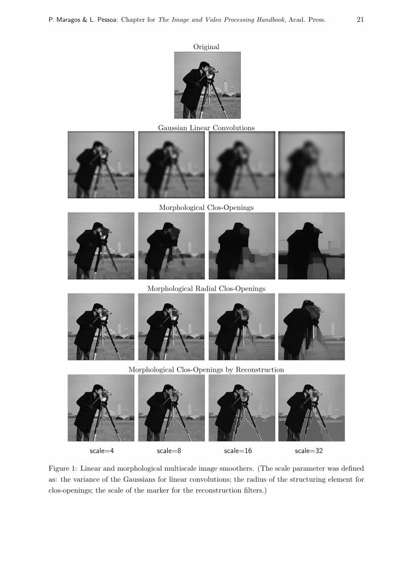
where the sets Lθ are rotated versions of a line segment L at various angles θ ∈ [0, 2π). This hasthe effect of preserving an object in f if this object is left unchanged after the opening by Lθ in atleast one of the possible orientations θ. See Fig. 1 for examples.
There are numerous image enhancement problems where what is needed is suppresion of arbitrarily-shaped connected components in the input image whose areas (number of pixels) are smaller thana certain threshold n. This can be accomplished by the area opening of size n which, for binaryimages, keeps only the connected components whose area is ≥ n and eliminates the rest. The areaopening can also be extended to graylevel images.
Consider now a set X =⋃
iXi as a union of disjoint connected components Xi and let M⊆Xj
be a marker in the j-th component; i.e., M could be a single point or some feature set in X thatlies only in Xj . Let us define the opening by reconstruction as the operator
MRX(M) ≡ connected component of X containing M . (22)
This is a lattice opening that from the input set M yields as output exactly the component Xj
containing the marker. Its output is called the morphological reconstruction of the component fromthe marker. It can extract large-scale components of the image from knowledge only of a smallermarker inside them. An algorithm to implement the opening by reconstruction is based on theconditional dilation of M by B within X:
δB|X(M) ≡ (M⊕B) ∩X (23)
If B is a disk with a radius smaller than the distance between Xj and any of the other components,then by iterating this conditional dilation we can obtain in the limit
limn→∞ (δB|X ...(δB|X(δB|X(M)))︸ ︷︷ ︸
n times
= MRX(M)
the whole component Xj . Replacing the binary with graylevel images, the set dilation with functiondilation, and ∩ with ∧ yields the graylevel opening by reconstruction. Openings (and closings)by reconstruction have proven to be extremely useful for image simplification because they cansuppress small features and keep only large-scale objects without any smoothing of their boundaries.Examples are shown in Fig. 1.
3.1.2 Multiscale Morphological Smoothers
Multiscale image analysis has recently emerged as a useful framework for many computer vision andimage processing tasks, including (i) noise suppression at various scales and (ii) feature detectionat large scales followed by refinement of their location or value at smaller scales. Most of theprevious work in this area was based on a linear multiscale smoothing, i.e., convolutions with aGaussian with a variance proportional to scale. However, these linear smoothers blur or shift imageedges, as shown in Fig. 1. In contrast, there is a variety of nonlinear smoothing filters, includingthe morphological openings and closings that can provide a multiscale image ensemble [17, 8] andavoid the above shortcomings of linear smoothers. For example, Fig. 1 shows three types of clos-openings (i.e., cascades of openings followed by closings): 1) Flat clos-openings by a 2D disk-like
8 P. Maragos & L. Pessoa: Chapter for The Image and Video Processing Handbook, Acad. Press.
structuring element which preserve the vertical image edges but may distort horizontal edges byfitting the shape of the structuring element. 2) Radial flat clos-openings that preserve both thevertical edges as well as any line features along the directions (0o, 45o, 90o, 135o) of the four linesegments used as structuring elements. 3) Gray-level clos-openings by reconstruction which areespecially useful because they can extract the exact outline of a certain object by locking on itwhile smoothing out all its surroundings; the marker for the opening (closing) by reconstructionwas an erosion (dilation) of the original image by a disk of radius equal to scale.
The required building blocks for the above morphological smoothers are the multiscale dilationsand erosions. The simplest multiscale dilation and erosion of an image f(x) at scales t > 0 are theflat dilations/erosions of f by scaled versions tB = {tz : z ∈ B} of a unit-scale planar compactconvex set B (e.g., a disk, a rhombus, a square)
δ(x, t) ≡ (f⊕tB)(x) , ε(x, t) ≡ (f�tB)(x) (24)
which apply both to graylevel and binary images. One discrete approach to implement multiscaledilations and erosions is to use scale recursion, i.e., f⊕(n+ 1)B = (f⊕nB)⊕B where n = 0, 1, 2,...,and nB denotes the n-fold dilation of B with itself. An alternative and more recent approach thatuses continuous models for multiscale smoothing is based on partial differential equations (PDEs).This was inspired by the modeling of linear multiscale image smoothing via the isotropic heatdiffusion PDE ∂U/∂t = ∇2U , where U(x, t) is the convolution of the initial image f(x) = U(x, 0)with a Gaussian at scale t. Similarly, the multiscale dilation δ(x, t) of f by a disk of radious (scale)t can be gererated as a weak solution of the following nonlinear PDE
∂δ
∂t= ||∇δ|| (25)
with initial condition δ(x, 0) = f(x), where ∇ denotes the spatial gradient operator and || · ||is the Euclidean norm. The generating PDE for the erosion is ∂ε/∂t = −||∇ε||. A review andreferences of the PDE approach to multiscale morphology can be found in [6]. In general, thePDE approach yields very close approximations to Euclidean multiscale morphology with arbitrarysubpixel accuracy.
3.1.3 Noise Suppresion by Median and Alternating Sequential Filters
In their behavior as nonlinear smoothers, as shown in Fig. 2, the medians act similarly to an open-closing (f◦B)•B by a convex set B of diameter about half the diameter of the median window[7]. The open-closing has the advantages over the median that it requires less computation anddecomposes the noise suppression task into two independent steps, i.e., suppressing positive spikesvia the opening and negative spikes via the closing.
The popularity and efficiency of the simple morphological openings and closings to suppress im-pulse noise is supported by the following theoretical development [19]. Assume a class of sufficientlysmooth random input images which is the collection of all subsets of a finite mask W that are open(or closed) with respect to a set B and assign a uniform probability distribution on this collection.Then, a discrete binary input image X is a random realization from this collection; i.e., use ideasfrom random sets [17] to model X. Further, X is corrupted by a union (or intersection) noise N
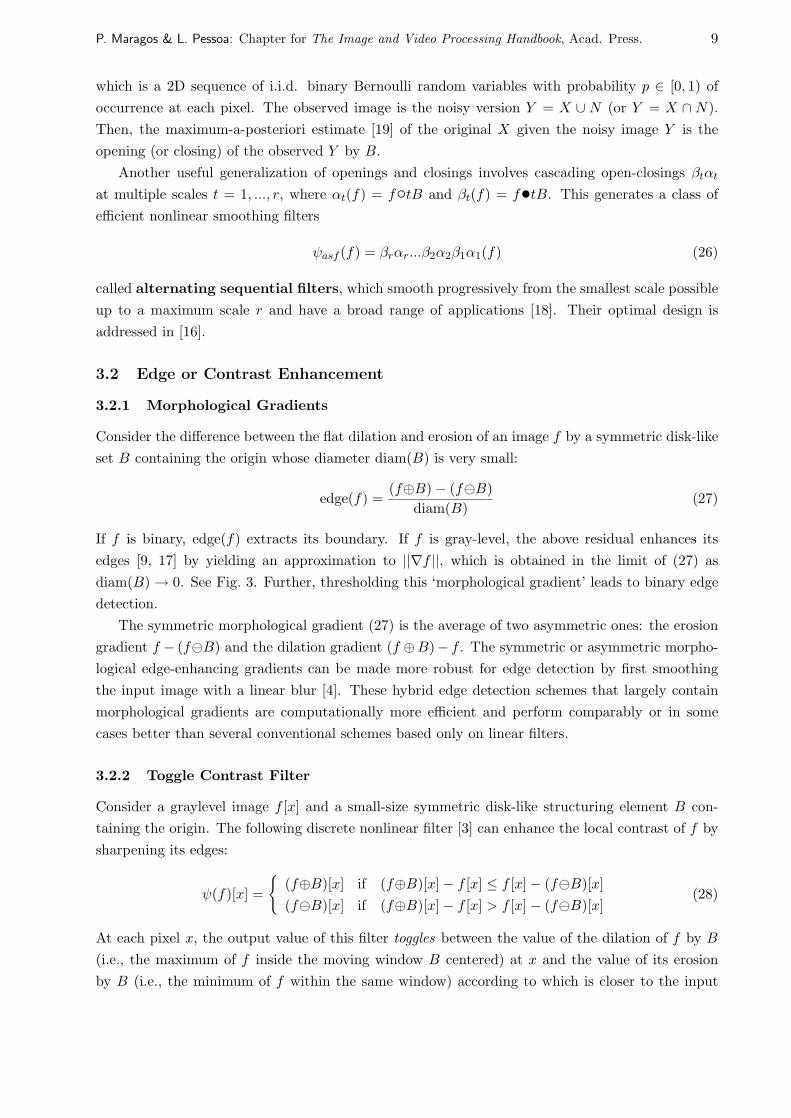
P. Maragos & L. Pessoa: Chapter for The Image and Video Processing Handbook, Acad. Press. 9
which is a 2D sequence of i.i.d. binary Bernoulli random variables with probability p ∈ [0, 1) ofoccurrence at each pixel. The observed image is the noisy version Y = X ∪ N (or Y = X ∩ N).Then, the maximum-a-posteriori estimate [19] of the original X given the noisy image Y is theopening (or closing) of the observed Y by B.
Another useful generalization of openings and closings involves cascading open-closings βtαt
at multiple scales t = 1, ..., r, where αt(f) = f◦tB and βt(f) = f•tB. This generates a class ofefficient nonlinear smoothing filters
ψasf (f) = βrαr...β2α2β1α1(f) (26)
called alternating sequential filters, which smooth progressively from the smallest scale possibleup to a maximum scale r and have a broad range of applications [18]. Their optimal design isaddressed in [16].
3.2 Edge or Contrast Enhancement
3.2.1 Morphological Gradients
Consider the difference between the flat dilation and erosion of an image f by a symmetric disk-likeset B containing the origin whose diameter diam(B) is very small:
edge(f) =(f⊕B) − (f�B)
diam(B)(27)
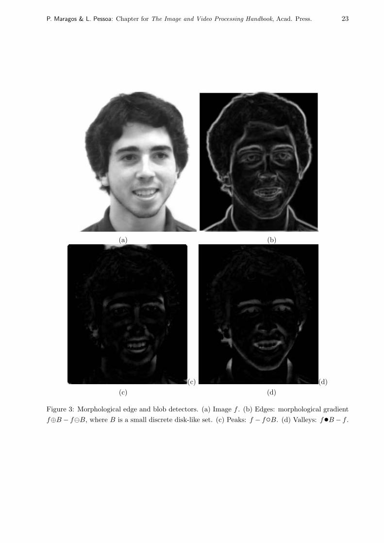
If f is binary, edge(f) extracts its boundary. If f is gray-level, the above residual enhances itsedges [9, 17] by yielding an approximation to ||∇f ||, which is obtained in the limit of (27) asdiam(B) → 0. See Fig. 3. Further, thresholding this ‘morphological gradient’ leads to binary edgedetection.
The symmetric morphological gradient (27) is the average of two asymmetric ones: the erosiongradient f − (f�B) and the dilation gradient (f ⊕B) − f . The symmetric or asymmetric morpho-logical edge-enhancing gradients can be made more robust for edge detection by first smoothingthe input image with a linear blur [4]. These hybrid edge detection schemes that largely containmorphological gradients are computationally more efficient and perform comparably or in somecases better than several conventional schemes based only on linear filters.
3.2.2 Toggle Contrast Filter
Consider a graylevel image f [x] and a small-size symmetric disk-like structuring element B con-taining the origin. The following discrete nonlinear filter [3] can enhance the local contrast of f bysharpening its edges:
ψ(f)[x] =
{(f⊕B)[x] if (f⊕B)[x] − f [x] ≤ f [x] − (f�B)[x](f�B)[x] if (f⊕B)[x] − f [x] > f [x] − (f�B)[x]
(28)
At each pixel x, the output value of this filter toggles between the value of the dilation of f by B(i.e., the maximum of f inside the moving window B centered) at x and the value of its erosionby B (i.e., the minimum of f within the same window) according to which is closer to the input
10 P. Maragos & L. Pessoa: Chapter for The Image and Video Processing Handbook, Acad. Press.
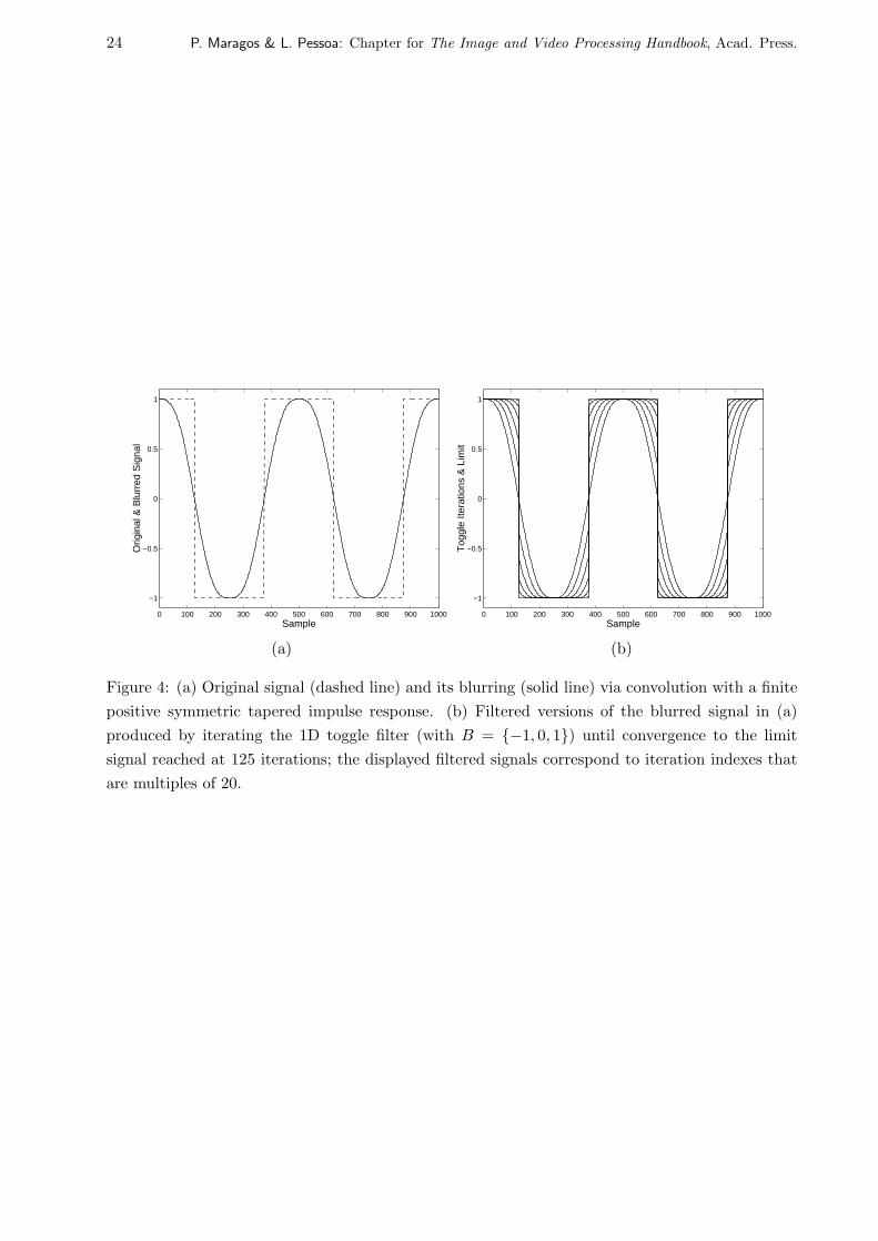
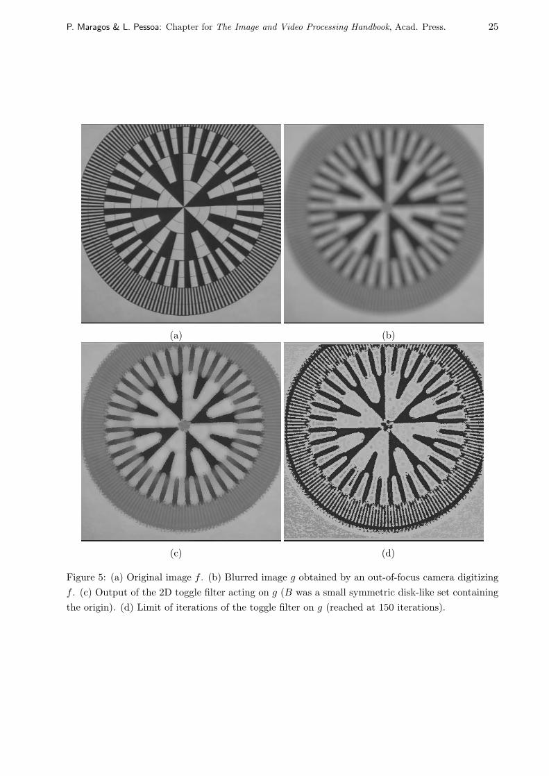
value f [x]. The toggle filter is usually applied not only once but is iterated. The more iterations,the more contrast enhancement. Further, the iterations converge to a limit (fixed point) [3] reachedafter a finite number of iterations. Examples are shown in Fig. 4 and Fig. 5.
As discussed in [15, 6], the above discrete toggle filter is closely related to the operation andnumerical algorithm behind a nonlinear (shock-wave) PDE proposed in [10] to deblur images and/orenhance their contrast by edge sharpening. For 1D images such a PDE is
∂u
∂t= −
∣∣∣∣∂u∂x∣∣∣∣ sign
(∂2u
∂x2
)(29)
Starting at t = 0, with the blurred image u(x, 0) = f(x) as the initial data, and running thenumerical algorithm implementing this PDE until some time t yields a filtered image u(x, t). Itsgoal is to restore blurred edges sharply, accurately and in a nonoscillatory way by propagatingshocks (i.e., discontinuities in the signal derivatives). Steady state is reached as t → ∞. Overconvex regions (∂2u/∂x2 > 0 ) this PDE acts as a 1D erosion PDE ∂u/∂t = −|∂u/∂x| which modelsmultiscale erosion of f(x) by the horizontal line segment [−t, t] and shifts parts of the graph ofu(x, t) with positive (negative) slope to the right (left) but does not move the extrema or inflectionpoints. Over concave regions (∂2u/∂x2 < 0) it acts as a 1D dilation PDE ∂u/∂t = |∂u/∂x| whichmodels multiscale dilation of f(x) by the same segment and reverses the direction of propagation.For certain piecewise-constant signals blurred via linear convolution with finite-window smoothtapered symmetric kernels, the shock filtering u(x, 0) �→ u(x,∞) can recover the original signal andthus achieve an exact deconvolution [10]; an example of such a case is shown in Fig. 4.
4 Morphological Filters for Detection
4.1 Morphological Correlation
Consider two real-valued discrete image signals f [x] and g[x]. Assume that g is a signal pattern tobe found in f . To find which shifted version of g “best” matches f a standard approach has beento search for the shift lag y that minimizes the mean squared error E2[y] =
∑x∈W (f [x+ y] − g[x])2
over some subset W of Z2. Under certain assumptions, this matching criterion is equivalent to
maximizing the linear cross-correlation Lfg[y] ≡ ∑x∈W f [x+ y]g[x] between f and g. A discussion
of linear template matching can be found in Chapter 3.1.Although less mathematical tractable than the mean squared error criterion, a statistically more
robust criterion is to minimize the mean absolute error
E1[y] =∑x∈W
|f [x+ y] − g[x]|
This mean absolute error criterion corresponds to a nonlinear signal correlation used for signalmatching; see [8] for a review. Specifically, since |a − b| = a + b − 2 min(a, b), under certainassumptions (e.g., if the error norm and the correlation is normalized by dividing it with the averagearea under the signals f and g), minimizing E1[y] is equivalent to maximizing the morphologicalcross-correlation
Mfg[y] ≡∑x∈W
min(f [x+ y], g[x]) (30)

P. Maragos & L. Pessoa: Chapter for The Image and Video Processing Handbook, Acad. Press. 11
It can be shown experimentally and theoretically that the detection of g in f is indicated by asharper matching peak in Mfg[y] than in Lfg[y]. In addition, the morphological (sum of minima)correlation is faster than the linear (sum of products) correlation. These two advantages of themorphological correlation coupled with the relative robustness of the mean absolute error criterionmake it promising for general signal matching.
4.2 Binary Object Detection and Rank Filtering
Let us approach the problem of binary image object detection in the presence of noise from theviewpoint of statistical hypothesis testing and rank filtering. Assume that the observed discretebinary image f [x] within a mask W has been generated under one of the following two probabilistichypotheses:
H0 : f [x] = e[x], x ∈ W .H1 : f [x] = |g[x− y] − e[x]|, x ∈ W .
Hypothesis H1 (H0) stands for ‘object present’ (‘object not present’) at pixel location y. The objectg[x] is a deterministic binary template. The noise e[x] is a stationary binary random field which isa 2D sequence of independent identically distributed (i.i.d.) random variables taking value 1 withprobability p and 0 with probability 1 − p, where 0 < p < 0.5. The mask W = G+y is a finite setof pixels equal to the region G of support of g shifted to location y at which the decision is taken.(For notational simplicity, G is assumed to be symmetric, i.e., G = Gr.) The absolute-differencesuperposition between g and e under H1 forces f to always have values 0 or 1. Intuitively, such asignal/noise superposition means that the noise e toggles the value of g from 1 to 0 and from 0 to1 with probability p at each pixel. This noise model can be viewed either as the common binarysymmetric channel noise in signal transmission or as a binary version of the salt-and-pepper noise.To decide whether the object g occurs at y we use a Bayes decision rule that minimizes the totalprobability of error and hence leads to the likelihood ratio test
Pr(f/H1)Pr(f/H0)
H1
>
<
H0
Pr(H0)Pr(H1)
(31)
where Pr(f/Hi) are the likelihoods of Hi with respect to the observed image f , and Pr(Hi) arethe a priori probabilities. This is equivalent to
Mfg[y] =∑x∈W
min(f [x], g[x− y])
H1
>
<
H0
θ =12
(log[Pr(H0)/Pr(H1)]
log[(1 − p)/p]+ card(G)
)(32)
Thus, the selected statistical criterion and noise model lead to compute the morphological (or equiv-alently linear) binary correlation between a noisy image and a known image object and compare itto a threshold for deciding whether the object is present.

12 P. Maragos & L. Pessoa: Chapter for The Image and Video Processing Handbook, Acad. Press.
Thus, optimum detection in a binary image f of the presence of a binary object g requirescomparing the binary correlation between f and g to a threshold θ. This is equivalent5 to performinga r-th rank filtering on f by a set G equal to the support of g, where 1 ≤ r ≤ card(G) and r is relatedto θ. Thus, the rank r reflects the area portion of (or a probabilistic confidence score for) the shiftedtemplate existing around pixel y. For example, if Pr(H0) = Pr(H1), then r = θ = card(G)/2 andhence the binary median filter by G becomes the optimum detector.
4.3 Hit-Miss Filter
The set erosion (3) can also be viewed as Boolean template matching since it gives the center pointsat which the shifted structuring element fits inside the image object. If we now consider a set Aprobing the image object X and another set B probing the background Xc, the set of points atwhich the shifted pair (A,B) fits inside the image X is the hit-miss transformation of X by(A,B):
X⊗(A,B) ≡ {x : A+x⊆X, B+x⊆Xc} (33)
In the discrete case, this can be represented by a Boolean product function whose uncomplemented(complemented) variables correspond to points of A (B). It has been used extensively for binaryfeature detection [17]. It can actually model all binary template matching schemes in binary patternrecognition that use a pair of a positive and a negative template [13].
In the presence of noise, the hit-miss filter can be made more robust by replacing the erosionsin its definitions with rank filters that do not require an exact fitting of the whole template pair(A,B) inside the image but only a part of it.
4.4 Morphological Peak/Valley Feature Detection
Residuals between openings or closings and the original image offer an intuitively simple and math-ematically formal way for peak or valley detection. Specifically, subtracting from an input imagef its opening by a compact convex set B yields an output consisting of the image peaks whosesupport cannot contain B. This is the top-hat transformation [9]
peak(f) = f − (f◦B) (34)
that has found numerous applications in geometric feature detection [17]. It can detect bright blobs,i.e., regions with significantly brighter intensities relative to the surroundings. The shape of thedetected peak’s support is controlled by the shape of B, whereas the scale of the peak is controlledby the size of B. Similarly, to detect dark blobs, modeled as image intensity valleys, we can use thevalley detector
valley(f) = (f•B) − f (35)
See Fig. 3 for examples.
5An alternative implementation and view of binary rank filtering is via thresholded convolutions, where a binaryimage is linearly convolved with the indicator function of a set G with n = card(G) pixels and then the result isthresholded at an integer level r between 1 and n; this yields the output of the r-th rank filter by G acting on theinput image.

P. Maragos & L. Pessoa: Chapter for The Image and Video Processing Handbook, Acad. Press. 13
The morphological peak/valley detectors are simple, efficient, and have some advantages overcurvature-based approaches. Their applicability in situations where the peaks or valleys are notclearly separated from their surroundings is further strengthened by generalizing them in the fol-lowing way. The conventional opening in (34) is replaced by a general lattice opening such as anarea opening or opening by reconstruction. This generalization allows a more effective estimationof the image background surroundings around the peak and hence a better detection of the peak.
5 Optimal Design of Morphological Filters for Enhancement
5.1 Brief Survey of Existing Design Approaches
Morphological and rank/stack filters are useful for image enhancement and are closely related sincethey can all be represented as maxima of morphological erosions [7]. Despite the wide applicationof these nonlinear filters, very few ideas exist for their optimal design. The current four mainapproaches are: (a) designing morphological filters as a finite union of erosions [5] based on themorphological basis representation theory (outlined in Section 2.3); (b) designing stack filters viathreshold decomposition and linear programming [1]; (c) designing morphological networks usingeither voting logic and rank tracing learning or simulated annealing [20]; (d) designing morpholog-ical/rank filters via a gradient-based adaptive optimization [14]. Approach (a) is limited to binaryincreasing filters. Approach (b) is limited to increasing filters processing nonnegative quantizedsignals. Approach (c) needs a long time to train and convergence is complex. In contrast, approach(d) is more general since it applies to both increasing and non-increasing filters and to both binaryand real-valued signals. The major difficulty involved is that rank functions are not differentiable,which imposes a deadlock on how to adapt the coefficients of morphological/rank filters using agradient-based algorithm. The methodology described in this section is an extension and improve-ment to the design methodology (d), leading to a new approach that is simpler, more intuitive andnumerically more robust.
For various signal processing applications it is sometimes useful to mix in the same system bothnonlinear and linear filtering strategies. Thus, hybrid systems, composed by linear and nonlinear(rank-type) sub-systems, have frequently been proposed in the research literature. A typical exam-ple is the class of L-filters that are linear combinations of rank filters. Several adaptive algorithmshave also been developed for their design, which illustrated the potential of adaptive hybrid filtersfor image processing applications, especially in the presence of non-Gaussian noise.
Given the applicability of hybrid systems and the relatively few existing ideas to design theirnonlinear part, in this section we present a general class of nonlinear systems, called morphologi-cal/rank/linear (MRL) filters [11], that contains as special cases morphological, rank, and linearfilters, and we develop an efficient method for their adaptive optimal design. MRL filters consist ofa linear combination between a morphological/rank filter and a linear FIR filter. Their nonlinearcomponent is based on a rank function, from which the basic morphological operators of erosionand dilation can be obtained as special cases.
14 P. Maragos & L. Pessoa: Chapter for The Image and Video Processing Handbook, Acad. Press.
5.2 MRL Filters
We shall use a vector notation to represent the values of the 1D or 2D sampled signal (after someenumeration of the signal samples) inside an n-point moving window. Let x = (x1, x2, · · · , xn) inR
n represent the input signal segment and y be the output value from the filter. The MRL filteris defined as the shift-invariant system whose local signal transformation rule x �→ y is given by
y ≡ λα+ (1 − λ)β ,α = Rr(x+ a) = Rr(x1 + a1, x2 + a2, · · · , xn + an) ,
β = x · bT = x1b1 + x2b2 + · · · + xnbn ,
(36)
where λ ∈ R, a, b ∈ Rn, and ‘(·)T ’ denotes transposition. Rr(t) is the r-th rank function of
t ∈ Rn. It is evaluated by sorting the components of t = (t1, t2, · · · , tn) in decreasing order, t(1) ≥
t(2) ≥ · · · ≥ t(n), and picking the r-th element of the sorted list; i.e., Rr(t) ≡ t(r) , r = 1, 2, · · · , n.The vector b = (b1, b2, · · · , bn) corresponds to the coefficients of the linear FIR filter, and the vectora = (a1, a2, · · · , an) represents the coefficients of the morphological/rank filter. We call a the “struc-turing element” because for r = 1 and r = n the rank filter becomes the morphological dilationand erosion by a structuring function equal to ±a within its support. For 1 < r < n, we use a togeneralize the standard unweighted rank operations to filters with weights. The median is obtainedwhen r = �n/2 + 1�. Besides these two sets of weights, the rank r and the mixing parameter λ willalso be included in the training process for the filter design. If λ ∈ [0, 1], the MRL-filter becomes aconvex combination of its components, so that when we increase the contribution of one component,the other one decreases. From (36) it follows that, computing each output sample requires 2n+ 1additions, n+ 2 multiplications and an n-point sorting operation.
Due to the use of a gradient-based adaptive algorithm, derivatives of rank functions will beneeded. Since these functions are not differentiable in the common sense, we will propose a simpledesign alternative using ‘rank indicator vectors’ and ‘smoothed impulses’. We define the unit samplefunction q(v), v ∈ R, as
q(v) ≡{
1 , if v = 00 , otherwise
(37)
Applying q to all components of a vector v ∈ Rn, yields a vector unit sample function
Q(v) ≡ (q(v1), q(v2), · · · , q(vn)).
Given a vector t = (t1, t2, · · · , tn) in Rn, and a rank r ∈ {1, 2, · · · , n}, the r-th rank indicator
vector c of t is defined by
c(t, r) ≡ Q(z1 − t)Q(z1 − t) · 1T
, z = Rr(t) , (38)
where 1 = (1, 1, · · · , 1). Thus, the rank indicator vector marks the locations in t where the z valueoccurs. It has many interesting properties [11], which include the following. It has unit area:
c · 1T = 1
It yields an inner-product representation of the rank function:
c · tT = Rr(t)

P. Maragos & L. Pessoa: Chapter for The Image and Video Processing Handbook, Acad. Press. 15
Further, for r fixed, if c is constant in a neighborhood of some t0, then the r-th rank function Rr(t)is differentiable at t0 and
∂Rr(t)∂t
∣∣∣∣t=t0
= c(t0, r). (39)
At points in whose neighborhood c is not constant, the rank function is not differentiable.At points where the function z = Rr(t) is not differentiable, a possible design choice is to assign
the vector c as a one-sided value of the discontinuous ∂z/∂t. Further, since the rank indicator vectorwill be used to estimate derivatives and it is based on the discontinuous unit sample function, asimple approach to avoid abrupt changes and achieve numerical robustness is to replace the unitsample function by a smoothed impulse qσ(v) that depends on a scale parameter σ ≥ 0 and hasat least the following required properties:
qσ(v) = qσ(−v) (symmetry)qσ(v) → q(v) ∀ v as σ → 0,qσ(v) → 1 ∀ v as σ → ∞.
(40)
Functions like exp[−1
2(v/σ)2]
or sech2(v/σ) are natural choices for qσ(v).From the filter definition (36), we see that our design goal is to specify a set of parameters
a, b, r and λ in such a way that some design requirement is met. However, instead of using theinteger rank parameter r directly in the training equations, we work with a real variable ρ implicitlydefined via the following rescaling
r ≡⌊n− n− 1
1 + exp(−ρ) + 0.5⌋, ρ ∈ R , (41)
where �· + 0.5� denotes the usual rounding operation and n is the dimension of the input signalvector x inside the moving window. Thus, the weight vector to be used in the filter design task isdefined by
w ≡ (a, ρ, b, λ) , (42)
but any of its components may be fixed during the process.
5.3 LMS Approach to Designing Optimal MRL Filters
Our framework for adaptive design is related to adaptive filtering, where the design is viewed asa learning process and the filter parameters are iteratively adapted until convergence is achieved.The usual approach to adaptively adjust the vector w, and therefore design the filter, is to define acost function J(w), estimate its gradient ∇J(w), and update w by the iterative (recursive) formula
w(i+ 1) = w(i) − µ0∇J(w)|w=w(i) , (43)
so that the value of the cost function tends to decrease at each step. The positive constant µ0 isusually called the step size and regulates the tradeoff between stability and speed of convergence ofthe iterative procedure. The iteration (43) starts with an initial guess w(0) and is terminated whensome desired condition is reached. This approach is commonly known as the method of steepestdescent.

16 P. Maragos & L. Pessoa: Chapter for The Image and Video Processing Handbook, Acad. Press.
As cost function J , for the i-th update w(i) of the weight vector, we use
J(w(i)) =1M
i∑k=i−M+1
e2(k) , (44)
where M = 1, 2, · · · is a memory parameter, and the instantaneous error
e(k) = d(k) − y(k) (45)
is the difference between the desired output signal d(k) and the actual filter output y(k) for thetraining sample k. The memory parameter M controls the smoothness of the updating process.If we are processing noiseless signals, it is sometimes better to simply set M = 1 (minimumcomputational complexity). On the other hand, if we are processing noisy signals, we should useM > 1 and sufficiently large to reduce the noise influence during the training process. Further, itis possible to make a training process convergent by using a larger value of M .
Hence, the resulting adaptation algorithm, called the averaged least mean square (LMS) algo-rithm, is
w(i+ 1) = w(i) +µ
M
i∑k=i−M+1
e(k)∂y(k)∂w
∣∣∣∣∣∣w=w(i)
, i = 0, 1, 2, · · · , (46)
where µ = 2µ0. From (42) and (36)
∂y
∂w=(∂y
∂a,∂y
∂ρ,∂y
∂b,∂y
∂λ
)=
[λ∂α
∂a, λ
∂α
∂ρ, (1 − λ)x, α− β
]. (47)
According to (39) and our design choice, we set
∂α
∂a= c =
Q(α1 − x− a)Q(α1 − x− a) · 1T
, α = Rr(x+ a). (48)
The final unknown is s = ∂α/∂ρ, which will be one more design choice. Notice from (41) and (36)that s ≥ 0. If all the elements of t = x + a are identical, then the rank r does not play any role,so that s = 0 whenever this happens. On the other hand, if only one element of t is equal to α,then variations in the rank r can drastically modify the output α; in this case s should assume amaximum value. Thus, a possible simple choice for s is
∂α
∂ρ= s ≡ 1 − 1
nQ(α1 − x− a) · 1T , α = Rr(x+ a) , (49)
where n is the dimension of x.Finally, to improve the numerical robustness of the training algorithm, we will frequently re-
place the unit sample function by smoothed impulses (obeying (40)), in which case an appro-priate smoothing parameter σ should be selected. A natural choice of a smoothed impulse isqσ(v) = exp[−1
2(v/σ)2], σ > 0. The choice of this nonlinearity will affect only the gradient estima-tion step in the design procedure (46). We should use small values of σ such that qσ(v) is closeenough to q(v). A possible systematic way to select the smoothing parameter σ could be to set|qσ(v)| ≤ ε for |v| ≥ δ, so that, for some desired ε and δ, σ = δ/
√ln(1/ε2).
Theoretical conditions for convergence of the training process (46) can be derived under thefollowing considerations. The goal is to find upper bounds µw to the step size µ, such that (46) can

P. Maragos & L. Pessoa: Chapter for The Image and Video Processing Handbook, Acad. Press. 17
converge if 0 < µ < µw. We assume the framework of system identification with noiseless signals,and consider the training process of only one element of w at a time, while the others are optimallyfixed. This means that given the original and transformed signals, and three parameters (sets) ofthe original w∗ = (a∗, ρ∗, b∗, λ∗) used to transform the input signal, we will use (46) to trackonly the fourth unknown parameter (set) of w∗ in a noiseless environment. If the training process(46) is convergent, then limi→∞ ‖w(i) −w∗‖ = 0, where ‖ · ‖ is some error norm. By analyzing thebehavior of ‖w(i)−w∗‖, under the above assumptions, conditions for convergence have been foundin [11].
5.4 Application of Optimal MRL Filters to Enhancement
The proper operation of the training process (46) has been verified in [11] through experimentsconfirming that, if the conditions for convergence are met, our design algorithm converges fast tothe real parameters of the MRL-filter within small error distances.
We illustrate its applicability to image enhancement via an experiment.6 The goal here it torestore an image corrupted by non-Gaussian noise. Hence, the input signal is a noisy image, and thedesired signal is the original (noiseless) image. The noisy image for training the filter was generatedby first corrupting the original image with a 47 dB additive Gaussian white noise, and then witha 10% multi-valued impulse noise. After the MRL-filter is designed, another noisy image (withsimilar type of perturbation) is used for testing. The optimal filter parameters were estimated afterscanning the image twice during the training process. We used the training algorithm (46) withM = 1 and µ = 0.1, and started the process with an unbiased combination between a flat medianand the identity, i.e.,
a0 =
0 0 00 0 00 0 0
, b0 =
0 0 00 1 00 0 0
, ρ0 = 0, λ0 = 0.5 .
The final trained parameters of the filter were:
a =
0.75 0.00 0.05−0.46 −0.01 0.71−0.09 −0.02 −0.51
, b =
0.01 0.19 −0.010.13 0.86 0.070.00 0.13 −0.02
, r = 5, λ = 0.98 ,
which represents a biased combination between a non-flat median filter and a linear FIR filter,where some elements of a and b present more influence in the filtering process.
Figure 6 shows the results of using the designed MRL-filter with a test image, and its comparisonwith a flat median filter of the same window size. The noisy image used for training is not includedthere because the (noisy) images used for training and testing are simply different realizations ofthe same perturbation process. Observe that the MRL-filter outperformed the median filter by
6Implementation details: The images are scanned twice during the training process, following a zig zag pathfrom top to bottom, and then from bottom to top. The local input vector x is obtained at each pixel via column-by-column indexing of the image values inside a n-point square window centered around the pixel. The vectors a
and b are indexed the same way. The unit sample function q(v) is approximated by qσ(v) = exp[− 1
2 (v/σ)2], with
σ = 0.001. The image values are normalized to be in the range [0, 1].

18 P. Maragos & L. Pessoa: Chapter for The Image and Video Processing Handbook, Acad. Press.
about 3 dB. Spatial error plots are also included which show that, the optimal MRL-filter preservesbetter the image structure since its corresponding spatial error is more uncorrelated than the errorof the median filter.
For the type of noise used in this experiment, we must have at least part of the original (noiseless)image, otherwise we would not be able to provide a good estimate to the optimal filter parametersduring the training process (46). In order to validate this point, we repeated the above experimentusing 100x100 sub-images of the training image (only 17% of the pixels), and the resulting MRL-filter still outperformed the median filter by about 2.3dB. There are situations, however, wherewe can use only the noisy image together with some filter constraints and design the filter that isclosest to the identity [14]. But this approach is only appropriate for certain types of impulse noise.
An exhaustive comparison of different filter structures for noise cancellation is beyond the scopeof this chapter. Nevertheless, this experiment was extended with the adaptive design of a 3x3 L-filter under the same conditions. Starting the L-filter with a flat median, even after scanning theimage four times during the training process, the resulting L-filter was just 0.2dB better than the(flat) median filter.
AcknowledgementPart of this chapter dealt with the authors’ research work which was supported by the US NationalScience Foundation under Grants MIPS-86-58150 and MIP-94-21677.

P. Maragos & L. Pessoa: Chapter for The Image and Video Processing Handbook, Acad. Press. 19
References
[1] E. J. Coyle and J. H. Lin, “Stack Filters and the Mean Absolute Error Criterion”, IEEE Trans.Acoust. Speech Signal Processing, vol. 36, pp. 1244-1254, Aug. 1988.
[2] H.J.A.M. Heijmans, Morphological Image Operators, Acad. Press, Boston, 1994.
[3] H. P. Kramer and J. B. Bruckner, “Iterations of a Nonlinear Transformation for Enhancementof Digital Images”, Pattern Recognition, vol. 7, pp. 53–58, 1975.
[4] J.S.J. Lee, R.M. Haralick and L.G. Shapiro, “Morphologic Edge Detection,” IEEE Trans. Rob.Autom., vol. RA-3, pp. 142-156, Apr. 1987.
[5] R. P. Loce and E. R. Dougherty, “Facilitation of Optimal Binary Morphological Filter De-sign via Structuring Element Libraries and Design Constraints”, Optical Engineering, vol. 31,pp. 1008-1025, May 1992.
[6] P. Maragos, “Partial Differential Equations in Image Analysis: Continuous Modeling, DiscreteProcessing”, Proc. 1998 European Signal Processing Conference (EUSIPCO), Rhodes, Greece.Published in: Signal Processing IX: Theories and Applications, vol. II, pp. 527–536, EURASIPPress, 1998.
[7] P. Maragos and R. W. Schafer, “Morphological Filters. Part I: Their Set-Theoretic Analysis andRelations to Linear Shift-Invariant Filters. Part II: Their Relations to Median, Order-Statistic,and Stack Filters,” IEEE Trans. Acoust. Speech, Signal Process., vol. 35, pp.1153–1184, Aug.1987; ibid, vol. 37, p. 597, Apr. 1989.
[8] P. Maragos and R. W. Schafer, “Morphological Systems for Multidimensional Signal Process-ing”, Proc. IEEE, vol. 78, pp. 690–710, April 1990.
[9] F. Meyer, “Contrast Feature Extraction”, Proc. 1977 European Symp. on Quantitative Analy-sis of Microstructures in Materials Science, Biology and Medicine, France. Published in: Spe-cial Issues of Practical Metallography, J.L. Chermant, ed., Riederer-Verlag, Stuttgart, 1978,pp. 374-380.
[10] S. Osher and L. I. Rudin, “Feature-Oriented Image Enhancement Using Schock Filters”, SIAMJ. Numer. Anal., vol. 27, pp. 919–940, Aug. 1990.
[11] L. F. C. Pessoa and P. Maragos, “MRL-Filters: A General Class of Nonlinear Systems andTheir Optimal Design for Image Processing,” IEEE Trans. Image Processing, vol. 7, pp. 966–978, July 1998.
[12] K. Preston, Jr., and M.J.B. Duff, Modern Cellular Automata, Plenum Press, 1984.
[13] A. Rosenfeld and A. C. Kak, Digital Picture Processing, Vols. 1 & 2, Acad. Press, NY, 1982.
[14] P. Salembier, “Adaptive Rank Order Based Filters,” Signal Processing, vol. 27, pp. 1–25, 1992.

20 P. Maragos & L. Pessoa: Chapter for The Image and Video Processing Handbook, Acad. Press.
[15] J.G.M. Schavemaker, M.J.T. Reinders and R. Van den Boomgaard, “Image Sharpening byMorphological Filtering”, Proc. IEEE Workshop on Nonlinear Signal & Image Processing,MacKinac Island, Michigan, Sep. 1997.
[16] D. Schonfeld and J. Goutsias, “Optimal Morphological Pattern Restoration from Noisy BinaryImages”, IEEE Trans. Pattern Anal. Machine Intellig., vol. 13, pp. 14-29, Jan. 1991.
[17] J. Serra, Image Analysis and Mathematical Morphology, Acad. Press, NY, 1982.
[18] J. Serra, ed., Image Analysis and Mathematical Morphology, Vol.2: Theoretical Advances,Acad. Press, NY, 1988.
[19] N. D. Sidiropoulos, J. S. Baras and C. A. Berenstein, “Optimal Filtering of Digital Binary Im-ages Corrupted by Union/Intersection Noise”, IEEE Trans. Image Processing, vol. 3, pp. 382–403, July 1994.
[20] S. S. Wilson, “Training Structuring Elements in Morphological Networks”, in MathematicalMorphology in Image Processing, E.R. Dougherty, ed., Marcel Dekker, NY, 1993.
P. Maragos & L. Pessoa: Chapter for The Image and Video Processing Handbook, Acad. Press. 21
Original
Gaussian Linear Convolutions
Morphological Clos-Openings
Morphological Radial Clos-Openings
Morphological Clos-Openings by Reconstruction
scale=4 scale=8 scale=16 scale=32
Figure 1: Linear and morphological multiscale image smoothers. (The scale parameter was definedas: the variance of the Gaussians for linear convolutions; the radius of the structuring element forclos-openings; the scale of the marker for the reconstruction filters.)

22 P. Maragos & L. Pessoa: Chapter for The Image and Video Processing Handbook, Acad. Press.
(a) (b)
(c) (d)
Figure 2: (a) Original clean image. (b) Noisy image obtained by corrupting the original withtwo-level salt-and-pepper noise occuring with probability 0.1 (PSNR=18.9 dB). (c) Open-closingof noisy image by a 2 × 2-pel square (PSNR=25.4 dB). (d) Median of noisy image by a 3 × 3-pelsquare (PSNR=25.4 dB).
P. Maragos & L. Pessoa: Chapter for The Image and Video Processing Handbook, Acad. Press. 23
(a) (b)
(c) (d)(c) (d)
Figure 3: Morphological edge and blob detectors. (a) Image f . (b) Edges: morphological gradientf⊕B − f�B, where B is a small discrete disk-like set. (c) Peaks: f − f◦B. (d) Valleys: f•B − f .
24 P. Maragos & L. Pessoa: Chapter for The Image and Video Processing Handbook, Acad. Press.
0 100 200 300 400 500 600 700 800 900 1000
−1
−0.5
0
0.5
1
Orig
inal
& B
lurr
ed S
igna
l
Sample0 100 200 300 400 500 600 700 800 900 1000
−1
−0.5
0
0.5
1
Tog
gle
Itera
tions
& L
imit
Sample
(a) (b)
Figure 4: (a) Original signal (dashed line) and its blurring (solid line) via convolution with a finitepositive symmetric tapered impulse response. (b) Filtered versions of the blurred signal in (a)produced by iterating the 1D toggle filter (with B = {−1, 0, 1}) until convergence to the limitsignal reached at 125 iterations; the displayed filtered signals correspond to iteration indexes thatare multiples of 20.
P. Maragos & L. Pessoa: Chapter for The Image and Video Processing Handbook, Acad. Press. 25
(a) (b)
(c) (d)
Figure 5: (a) Original image f . (b) Blurred image g obtained by an out-of-focus camera digitizingf . (c) Output of the 2D toggle filter acting on g (B was a small symmetric disk-like set containingthe origin). (d) Limit of iterations of the toggle filter on g (reached at 150 iterations).

26 P. Maragos & L. Pessoa: Chapter for The Image and Video Processing Handbook, Acad. Press.
ORIGINAL TEST (19.3dB)
(a) (b)MEDIAN FILTER (25.7dB) MRL-FILTER (28.5dB)
(c) (d)SPATIAL ERROR / MEDIAN SPATIAL ERROR / MRL-FILTER
(e) (f)
Figure 6: (a) Original clean texture image (240x250). (b) Noisy image: Image (a) corrupted by ahybrid 47dB additive Gaussian white noise and 10% multi-valued impulse noise (PSNR = 19.3dB).(c) Noisy image restored by a flat 3x3 median filter (PSNR = 25.7dB). (d) Noisy image restoredby the designed 3x3 MRL-filter (PSNR = 28.5dB). (e) Spatial error map of the flat median filter;lighter areas indicate higher errors. (f) Spatial error map of the MRL-filter.