More PBM

Ruth Aylett

Overview

Collisions Deformable objects

– Hookes law– Cloth– Flesh

Fluids Plants Physics engines

Collision response

When objects collide they apply forceson each other

Collisions can be:– elastic, where no kinetic energy is lost

during the collision– inelastic, where kinetic energy is lost

Collision response

Consider a collision between 2 balls An impulse force, P, acts for a very

short timem1 ( v1

after - v1before ) = -f

m2 ( v2after - v2

before ) = f

Thereforem1v1

after + m2v2after = m1v1

before +m2v2

before

f

f

v1

v2

m1

m2

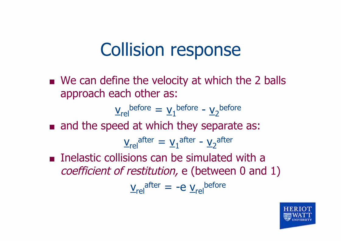
Collision response

We can define the velocity at which the 2 ballsapproach each other as:

vrelbefore = v1

before - v2before

and the speed at which they separate as:vrel

after = v1after - v2

after

Inelastic collisions can be simulated with acoefficient of restitution, e (between 0 and 1)

vrelafter = -e vrel

before

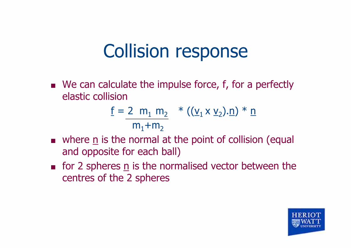
Collision response

We can calculate the impulse force, f, for a perfectlyelastic collision

f = 2 m1 m2 * ((v1 x v2).n) * n

m1+m2

where n is the normal at the point of collision (equaland opposite for each ball)

for 2 spheres n is the normalised vector between thecentres of the 2 spheres

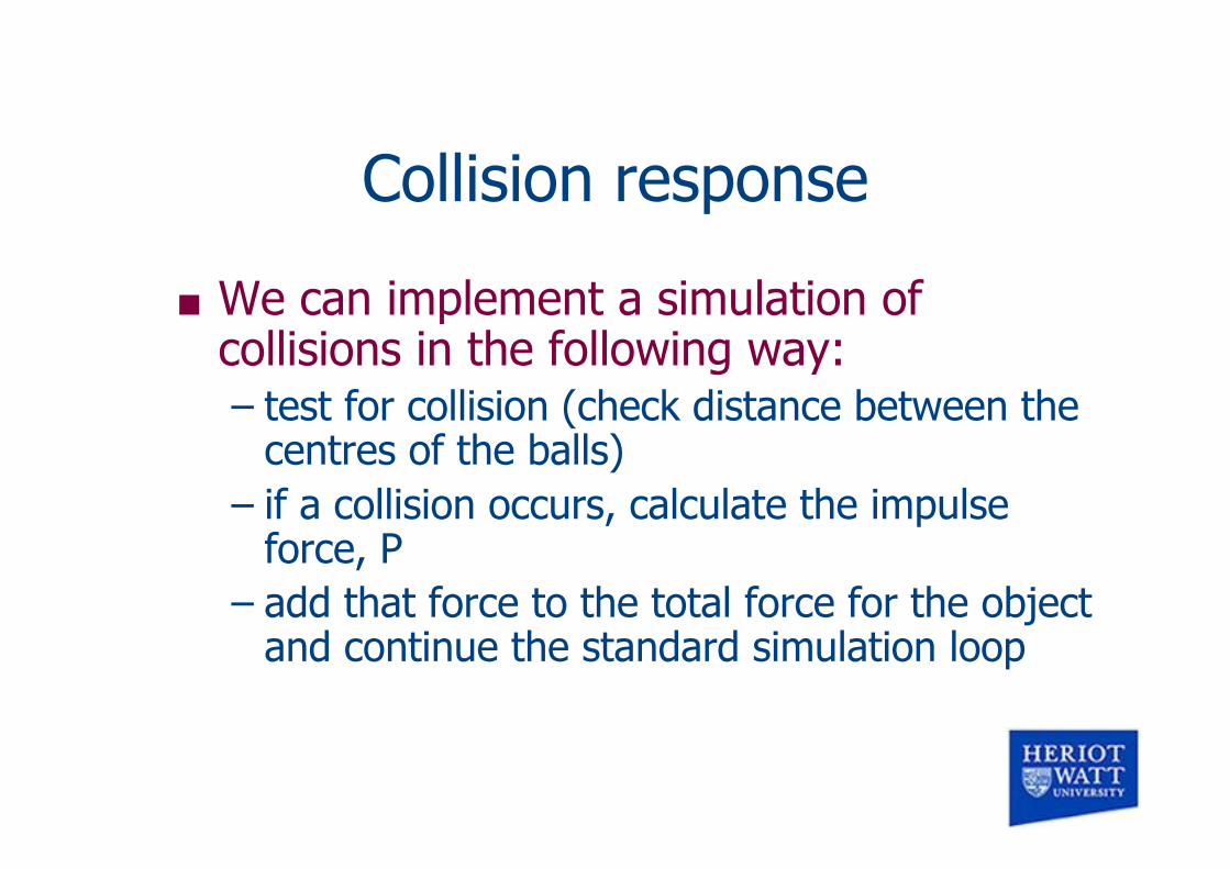
Collision response

We can implement a simulation ofcollisions in the following way:– test for collision (check distance between the

centres of the balls)– if a collision occurs, calculate the impulse

force, P– add that force to the total force for the object

and continue the standard simulation loop

Deformable objects

Deformable or soft objects can also besimulated using physical laws– jelly– cloth– flesh

Deformable objects

Modelling Approach– Spring and dashpot elements– Hooke’s law– Replace polygon edges with springs– Extend to allow cutting and fracture

Hooke’s Law Theory

– Consider a spring with restlength, L

– Let the extension of the springbe δL

– Let the coefficient of restitutionbe k

L+δLL

Hooke’s Law

The force generated in the spring isgiven by:

f = -k δL L

– The same expression works for springcompression, except δL is negative

– The dashpot element is included in thesystem to add some drag, reducing totalenergy

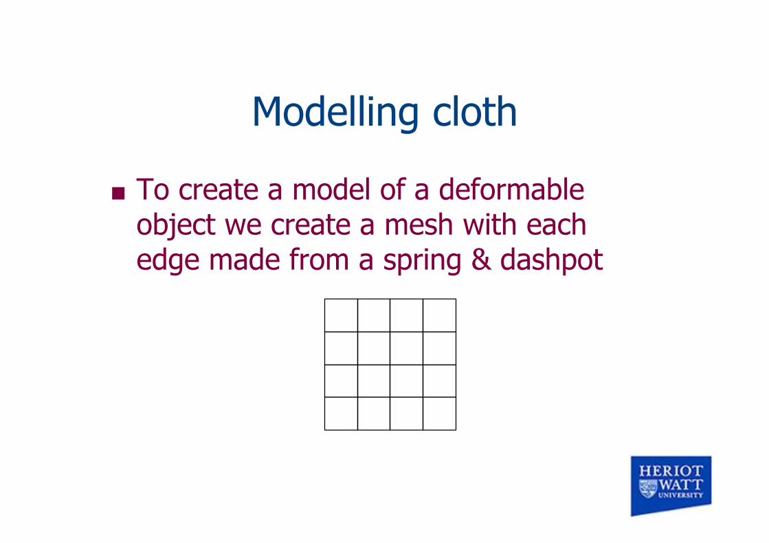
Modelling cloth

To create a model of a deformableobject we create a mesh with eachedge made from a spring & dashpot

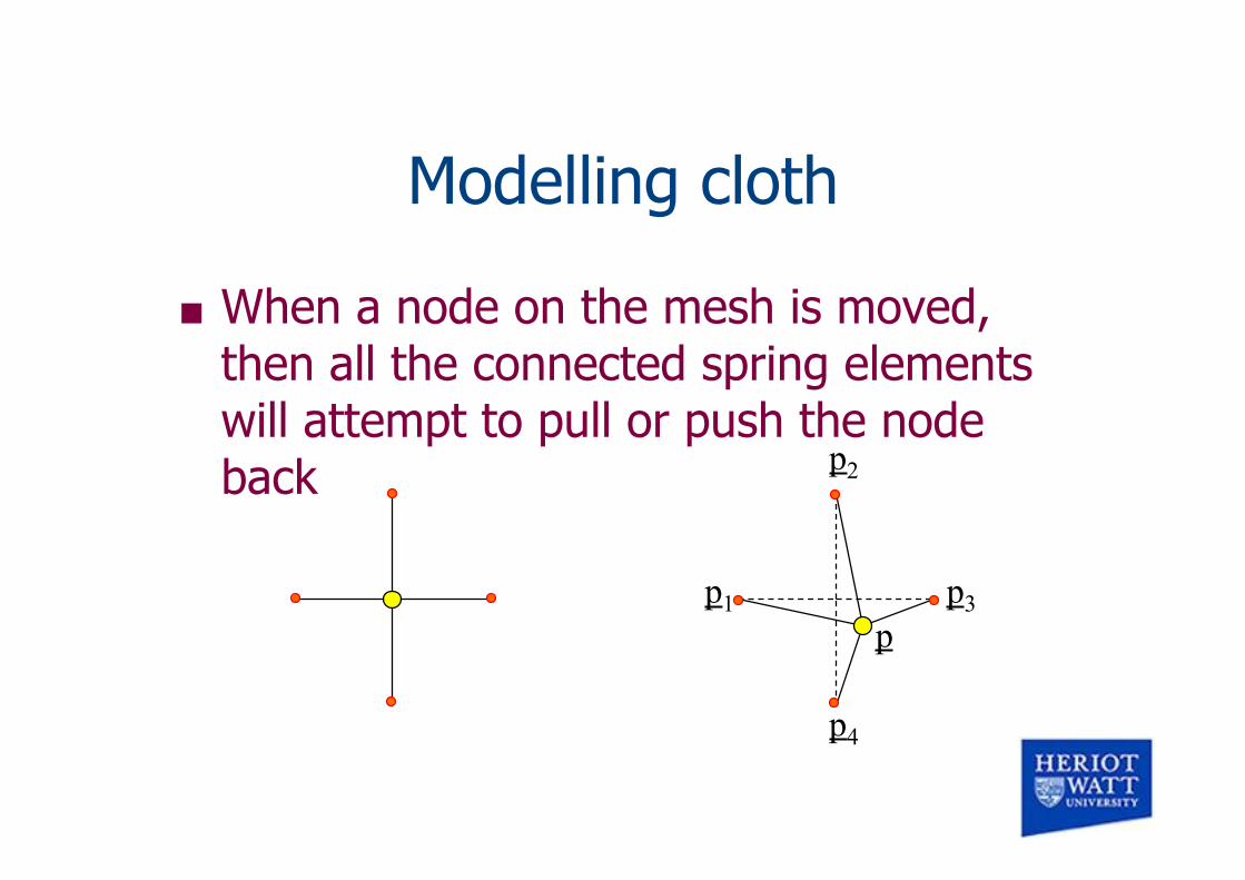
Modelling cloth

When a node on the mesh is moved,then all the connected spring elementswill attempt to pull or push the nodeback

p1 p3

p4

p2

p

Modelling cloth

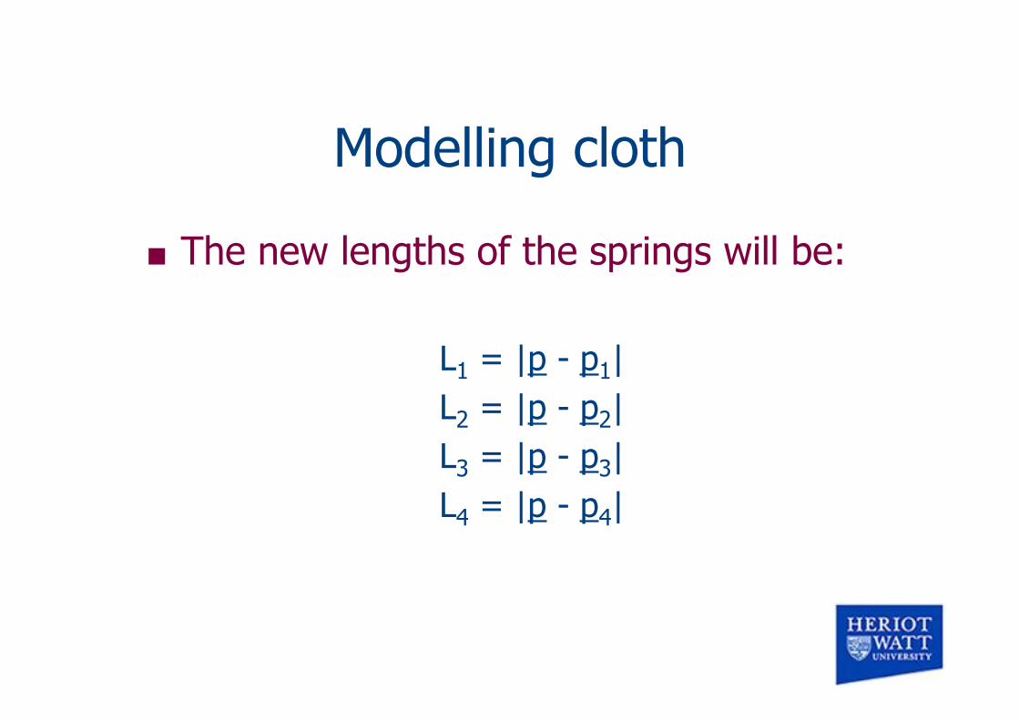
The new lengths of the springs will be:

L1 = |p - p1|L2 = |p - p2|L3 = |p - p3|L4 = |p - p4|

Modelling cloth

So the force on the node is:f1 + f2 + f3 + f4

wherefi = k * (Li - L) * ( pi - p )

L– note that each fi points in the direction of the

associated spring– once the forces have been added, the acceleration

can be found ( f / m = a)

normalised

Modelling cloth

We can the use our standard simulationloop to calculate new velocities andpositions for the node

When we have a mesh with many nodes wecalculate each step on all nodessimultaneously

Problems

Retaining the original structure– When these routines are applied to 3D objects,

they can easily lose their original shape

Solution– Record the original locations of the object’s nodes– Connect extra imaginary springs between the

original and current location of each node– Use a smaller value of k for these imaginary

springs

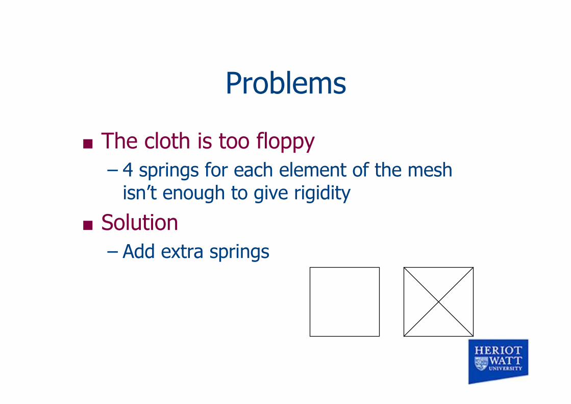
Problems

The cloth is too floppy– 4 springs for each element of the mesh

isn’t enough to give rigidity

Solution– Add extra springs

Modelling flesh

Case with no cutting / fracture– same as for cloth, but create a 3D mesh

with cubic elements

Modelling flesh

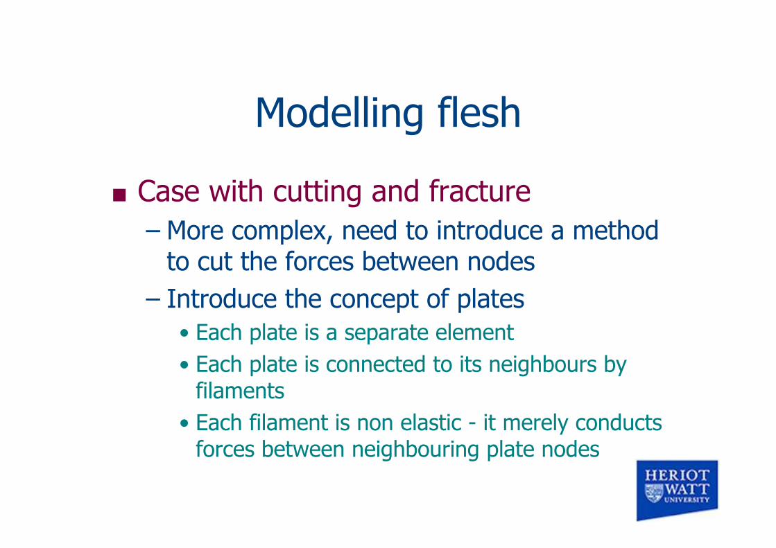
Case with cutting and fracture– More complex, need to introduce a method

to cut the forces between nodes– Introduce the concept of plates

• Each plate is a separate element• Each plate is connected to its neighbours by

filaments• Each filament is non elastic - it merely conducts

forces between neighbouring plate nodes

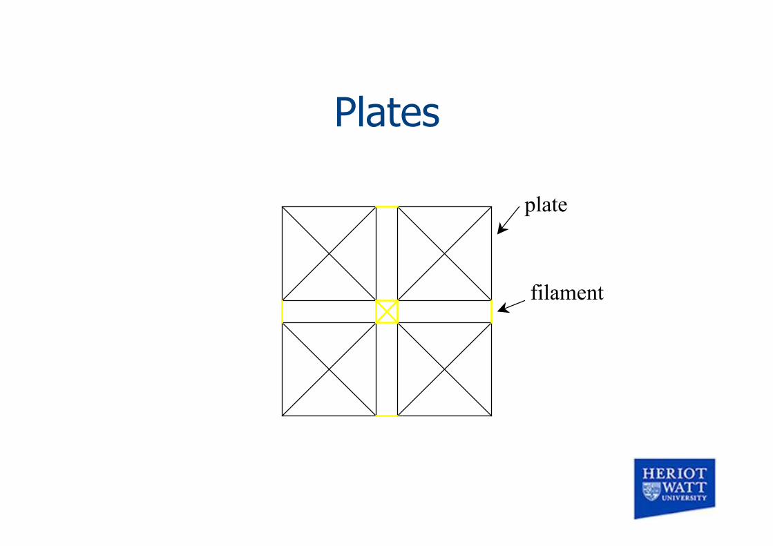
Plates

filament

plate

Controlling movement When no cut has taken place, the filaments

act to:– keep the nodes of the plates together– transmit forces from one node to another

Process is to calculate the forces on all nodeswithin each plate

If a node n1 from one plate and a node n2from another plate are connected then applythe forces from n1 to n2 and vice versa

Cutting

To cut the flesh, merely delete theconnections for appropriate filaments

To get the flesh to peel back whencutting / tearing, stretch the fleshbefore the simulation starts

Fracture

To simulate fracture (ripping, tearing), set amaximum force that the filament can conduct

If the total force conducted exceeds thefracture force then cut the filamentautomatically

By setting slightly different fracture forces foreach filament, we get irregular ripping effects

Problems

This method can be unstable Physical values have to be chosen

carefully Structure is very important

Fluid simulation

Three methods used for this:– Lattice Boltzmann Method (LBM);– Navier-Stokes (NS) solvers– Smoothed Particle Hydrodynamics (SPH)

All require substantial amounts ofcomputation

Simplified simulation also used: O’Brien& Hodgins

Computational Fluid Dynamics

Start with:– an arbitrary distribution of fluid– submerged or semi-submerged obstacles

Discretise the fluid volume into a 3Darray of box shaped elements

CFD

Velocity and pressure are:– defined throughout the fluid– updated throughout the simulation, using a

set of finite difference expressions– used to drive a height field equation to

create a surface for liquids

Boundary conditions

Boundary conditions can be used to– represent the edges of the mesh

• open, allowing fluid to flow in and out• closed

– represent the surface of a liquid– represent stationary obstacles

• sea bed• rocks

CFD

A variety of effects occur naturally from thismethod– waves

• reflection• refraction• diffraction

– rotational effects• eddies• vorticity• splashing

CFD

We can visually represent the fluid in 2ways– as a heightfield to represent the surface of

a liquid– as a collection of massless particles moving

through the fluid

Simple fluids

Navier Stokes provides an accurate, butcomputationally intensive solution

O’Brien and Hodgins provide analternative solution which is– simpler– less accurate– less detailed

Simplified representation

This method startsby considering thefluid body as a 2Dgrid rather than a 3Dgrid

Each elementrepresents a columnof fluid

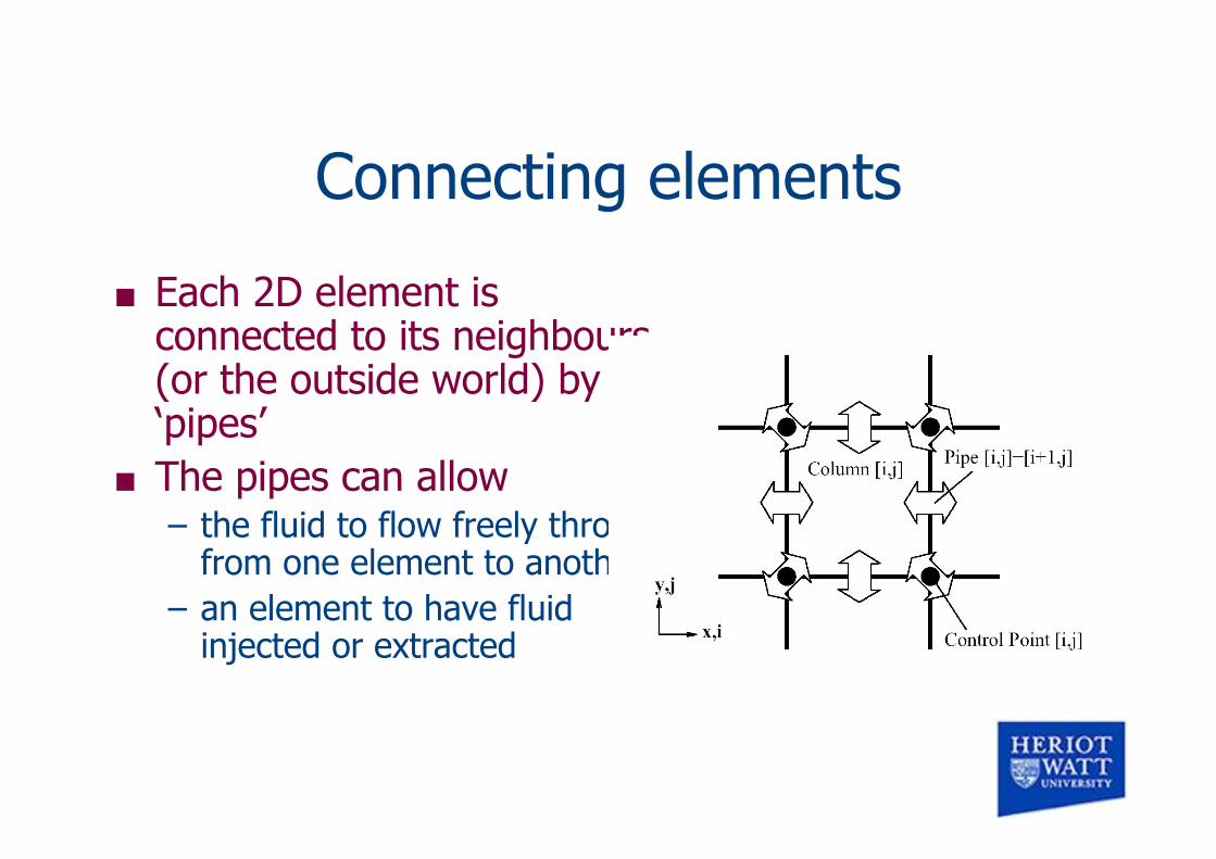
Connecting elements

Each 2D element isconnected to its neighbours(or the outside world) by 8‘pipes’

The pipes can allow– the fluid to flow freely through

from one element to another– an element to have fluid

injected or extracted

Fluid flow in pipes

The equations to determine the fluid flow in the pipes arebased on laws for hydrostatic pressure

The static pressure, H, in column i,j isHij = hijρg + p0 + Eij

where– h is the column height– g is gravity– ρ is the density of the fluid

– p0 is the atmospheric pressure– Eij is an external pressure applied by other objects

Constraints

We must also apply some constraints tothe system– The flows at each end of a pipe must be

equal and opposite– A column may not have a negative volume

Checking pipes

To ensure that no column has anegative volume– at the end of each update, the volume of

each column is tested– if the volume is negative, scale back the

pipes removing fluid from the column– repeat this procedure until all columns

have a non-negative volume

Setting the boundaries

Columns that are on the edge of thegrid have pipe connections to theoutside world

As there is no column at the other end,we must specify the flow in the pipe– barrier - set the flow to zero– fluid source - positive flow– fluid sink - negative flow

Fluid surface

We can representthe fluid with aheightfield surface

The surface is madeof triangles / quads,joining controlpoints

Plants

Apart from L-Systems (Lindenmeyer)can also model plants with voxels– A voxel is like a 3D pixel

Voxel space automata (Greene)

Voxel automata

This technique models plants withstochastic (random) growth

The space in which the plant grows isdiscretised into voxels

This technique is particularly good formodelling climbing / rambling plants

Growing the plant

The growth of the plant is affected by– occlusion (availability of light)– intersection (colliding with objects)– proximity (stick to walls, ramble over other

objects) These features are recorded within the

voxels

Probabilistic growth

The growth of the plant is probabilistic– test several different options for the next

bit of growth– for each option assess how good the

conditions are in the new position– choose and apply the best option

Light levels

Light levels are modelled with theassessment of occlusion

Each voxel assesses– amount of sunlight [ 0 .. 1 ]– amount of sky light [ 0 .. 1 ]

The amounts of these types of light arecalculated using ray casting

Light from the sky

Sky light– rays are cast from a voxel to points all over

the sky– if the ray hits an object before it gets to

the sky it is occluded [0]– otherwise it is exposed [1]– the average occlusion of all the rays can

then be calculated

Light from the sun

Sunlight– the 180 degree arc forming the trajectory

of the sun is determined– rays are cast from the voxel to the arc– rays are assessed for occlusion / exposure

The average occlusion is calculated

Growth cycle

Growth is affected by the amounts of lightavailable– The plant has acceptable max, min light levels

specified

Also assess all voxels for the presence ofobjects within each voxel (including bits ofthe plant)– Allows assessment of proximity, intersection

Once we know the conditions for all voxels,we can proceed with one stage of growth

Updating growth

Once a stage of growth has occurredthe voxel space is updated

Identify changes in– occlusion– intersection– proximity

Then another stage of growth can bestarted

Physics engines

Graphics programmers do not want to learnphysics– So specialist graphics libraries seemed a really

good idea

Now incorporated into most games engines– UT, Half-life, Unity etc– Also in Director, Flash (2D), Flex, Blender

Physics Processing Unit (2006)– A physics card in spirit of a graphics card– Physics processing now part of Nvidia and ATI

graphics cards

Physics engines available

Commercial– Havok

– www.havok.com

• Which took over Ipion• Used in Director, Half-life

– Now merged with Euphoria– NVidia took over Ageia Feb 2008

• PhysX engine and PPU

Free-or-nearly physics engines

Lots and lots! See http://en.wikipedia.org/wiki/Physics_engine– ODE - Open Dynamics Environment

• Rigid body dynamics, C/C++ API, mature, big community• http://opende.sourceforge.net/

Bullet• http://bulletphysics.org/wordpress/

The Physics Engine• http://www.thephysicsengine.com/

Newton game dynamics• http://www.newtondynamics.com/

Physics Abstraction Layer - PAL– Interface to variety of physics engines

• http://www.adrianboeing.com/pal/