more on randomization semi-definite programming and derandomization
TRANSCRIPT

WSPAA’06 Session 5
More on RandomizationSemidefinite Programming and Derandomization
Abner Chih-Yi Huang1
June 24, 2006
1Graduate student of M.S. degree CS program of Algorithm andBiocomputing Laboratory, National Tsing Hua University. [email protected]
Abner Chih-Yi Huang WSPAA’06 Session 5More on Randomization Semidefinite Programming and Derandomization
Outline
I Derandomization: The Method of The ConditionalProbabilities;
I Approximation Algorithms Based on SemidefiniteProgramming
I Introduction to Semidefinite ProgrammingI Application : MaxCut, Weighted-Max2SAT problem
Abner Chih-Yi Huang WSPAA’06 Session 5More on Randomization Semidefinite Programming and Derandomization
Derandomization
Derandomization.
Abner Chih-Yi Huang WSPAA’06 Session 5More on Randomization Semidefinite Programming and Derandomization

Why Do We Study Derandomization?
Why do we study derandomization since that randomizedalgorithms are so powerful?
Because independent random unbiased bits are hard to obtain.
Empirically a large number of randomized algorithms have beenimplemented and seem to work just fine, even without access toany source of true randomness. There are, essentially, two generalarguments to support the belief that BPP is “close” to P.
Abner Chih-Yi Huang WSPAA’06 Session 5More on Randomization Semidefinite Programming and Derandomization
De-randomization
I Removing randomization from randomized algorithms to buildequivalently powerful deterministic algorithms.
I One of general technique, method of the conditionalprobabilities.
I View a randomized algorithm A as a computation tree oninput x .
I Assume A independently perform r(|x |) random choices eachwith two possible outcomes, denoted 0 and 1.
I Each path form root to a leaf means a possible computation ofA .
Abner Chih-Yi Huang WSPAA’06 Session 5More on Randomization Semidefinite Programming and Derandomization
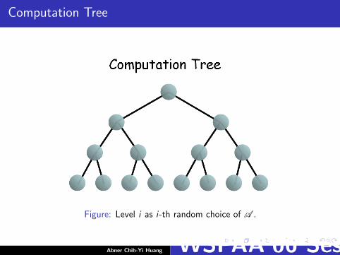
Computation Tree
Figure: Level i as i-th random choice of A .
Abner Chih-Yi Huang WSPAA’06 Session 5More on Randomization Semidefinite Programming and Derandomization

Computation Tree
Figure: Assign each node u, of level i , a binary string σ(u) of lengthi − 1 representing the random choices so far.
Abner Chih-Yi Huang WSPAA’06 Session 5More on Randomization Semidefinite Programming and Derandomization
Computation Tree
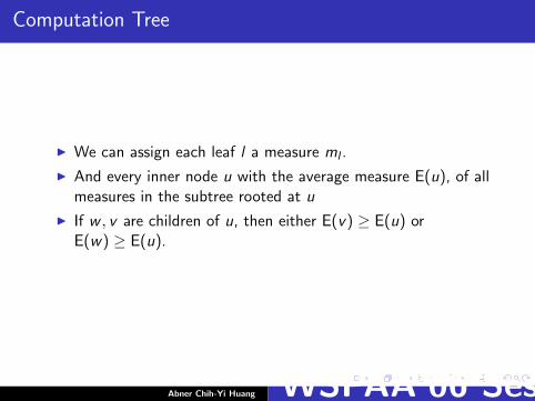
I We can assign each leaf l a measure ml .
I And every inner node u with the average measure E(u), of allmeasures in the subtree rooted at u
I If w , v are children of u, then either E(v) ≥ E(u) orE(w) ≥ E(u).
Abner Chih-Yi Huang WSPAA’06 Session 5More on Randomization Semidefinite Programming and Derandomization
Computation Tree
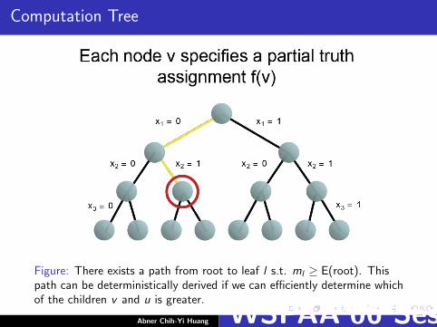
Figure: There exists a path from root to leaf l s.t. ml ≥ E(root). Thispath can be deterministically derived if we can efficiently determine whichof the children v and u is greater.
Abner Chih-Yi Huang WSPAA’06 Session 5More on Randomization Semidefinite Programming and Derandomization
Example: Weighted MaxSAT
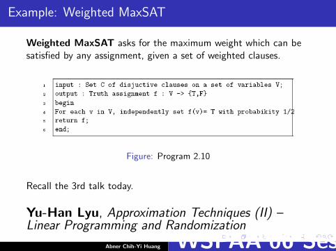
Weighted MaxSAT asks for the maximum weight which can besatisfied by any assignment, given a set of weighted clauses.
Figure: Program 2.10
Recall the 3rd talk today.
Yu-Han Lyu, Approximation Techniques (II) –Linear Programming and Randomization
Abner Chih-Yi Huang WSPAA’06 Session 5More on Randomization Semidefinite Programming and Derandomization
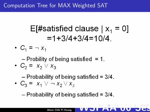
Computation Tree for MAX Weighted SAT
Abner Chih-Yi Huang WSPAA’06 Session 5More on Randomization Semidefinite Programming and Derandomization
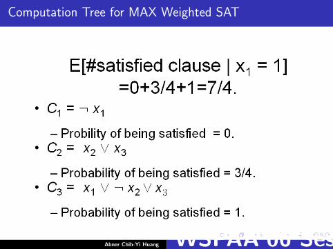
Computation Tree for MAX Weighted SAT
Abner Chih-Yi Huang WSPAA’06 Session 5More on Randomization Semidefinite Programming and Derandomization
Computation Tree for MAX Weighted SAT
Abner Chih-Yi Huang WSPAA’06 Session 5More on Randomization Semidefinite Programming and Derandomization

Computation Tree for MAX Weighted SAT
Abner Chih-Yi Huang WSPAA’06 Session 5More on Randomization Semidefinite Programming and Derandomization
Computation Tree for MAX Weighted SAT
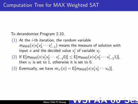
To derandomize Program 2.10,
(1) At the i-th iteration, the random variablemRWS(x |v ′1v ′2 · · · v ′i−1) means the measure of solution withinput x and the decided value v ′j of variable vj .
(2) If E[mRWS(x |v ′1v ′2 · · · v ′i−10)] ≤ E[mRWS(x |v ′1v ′2 · · · v ′i−11)],then vi is set to 1, otherwise it is set to 0.
(3) Eventually, we have mA (x) = E[mRWS(x |v ′1v ′2 · · · vn)].
Abner Chih-Yi Huang WSPAA’06 Session 5More on Randomization Semidefinite Programming and Derandomization
Computation Tree for MAX Weighted SAT
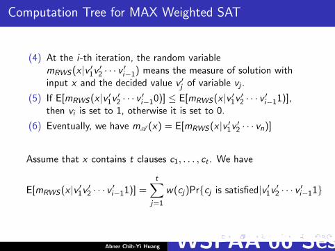
(4) At the i-th iteration, the random variablemRWS(x |v ′1v ′2 · · · v ′i−1) means the measure of solution withinput x and the decided value v ′j of variable vj .
(5) If E[mRWS(x |v ′1v ′2 · · · v ′i−10)] ≤ E[mRWS(x |v ′1v ′2 · · · v ′i−11)],then vi is set to 1, otherwise it is set to 0.
(6) Eventually, we have mA (x) = E[mRWS(x |v ′1v ′2 · · · vn)]
Assume that x contains t clauses c1, . . . , ct . We have
E[mRWS(x |v ′1v ′2 · · · v ′i−11)] =t∑
j=1
w(cj)Pr{cj is satisfied|v ′1v ′2 · · · v ′i−11}
Abner Chih-Yi Huang WSPAA’06 Session 5More on Randomization Semidefinite Programming and Derandomization
Computation Tree for MAX Weighted SAT
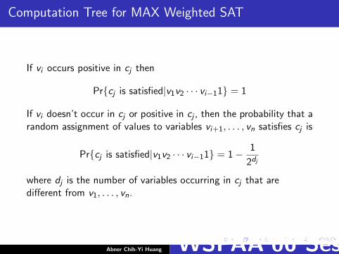
If vi occurs positive in cj then
Pr{cj is satisfied|v1v2 · · · vi−11} = 1
If vi doesn’t occur in cj or positive in cj , then the probability that arandom assignment of values to variables vi+1, . . . , vn satisfies cj is
Pr{cj is satisfied|v1v2 · · · vi−11} = 1− 1
2dj
where dj is the number of variables occurring in cj that aredifferent from v1, . . . , vn.
Abner Chih-Yi Huang WSPAA’06 Session 5More on Randomization Semidefinite Programming and Derandomization
Computation Tree for MAX Weighted SAT
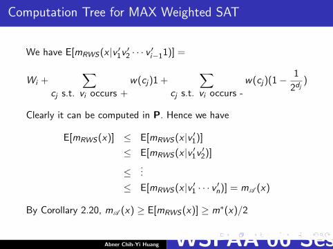
We have E[mRWS(x |v ′1v ′2 · · · v ′i−11)] =
Wi +∑
cj s.t. vi occurs +
w(cj)1 +∑
cj s.t. vi occurs -
w(cj)(1−1
2dj)
Clearly it can be computed in P. Hence we have
E[mRWS(x)] ≤ E[mRWS(x |v ′1)]≤ E[mRWS(x |v ′1v ′2)]
≤...
≤ E[mRWS(x |v ′1 · · · v ′n)] = mA (x)
By Corollary 2.20, mA (x) ≥ E[mRWS(x)] ≥ m∗(x)/2
Abner Chih-Yi Huang WSPAA’06 Session 5More on Randomization Semidefinite Programming and Derandomization

Semidefinite Programming
Semidefinite Programming
Abner Chih-Yi Huang WSPAA’06 Session 5More on Randomization Semidefinite Programming and Derandomization
The Second Part: SDP
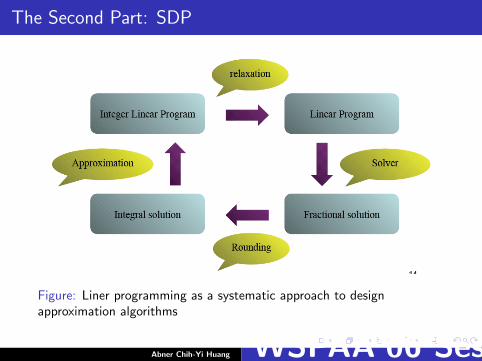
Figure: Liner programming as a systematic approach to designapproximation algorithms
Abner Chih-Yi Huang WSPAA’06 Session 5More on Randomization Semidefinite Programming and Derandomization
The Power of Liner Programming
Recall the 3rd talk today.
Yu-Han Lyu, ApproximationTechniques (II) – LinearProgramming andRandomization
Abner Chih-Yi Huang WSPAA’06 Session 5More on Randomization Semidefinite Programming and Derandomization
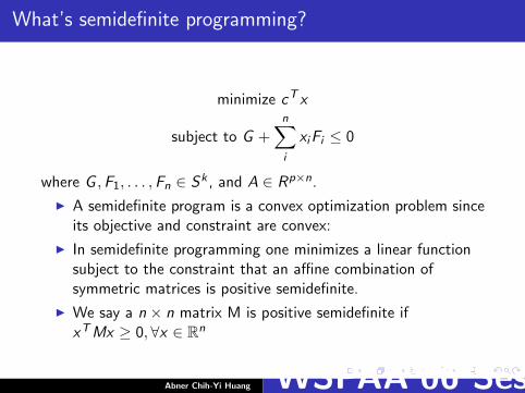
What’s semidefinite programming?
minimize cT x
subject to G +n∑i
xiFi ≤ 0
where G ,F1, . . . ,Fn ∈ Sk , and A ∈ Rp×n.
I A semidefinite program is a convex optimization problem sinceits objective and constraint are convex:
I In semidefinite programming one minimizes a linear functionsubject to the constraint that an affine combination ofsymmetric matrices is positive semidefinite.
I We say a n × n matrix M is positive semidefinite ifxTMx ≥ 0,∀x ∈ Rn
Abner Chih-Yi Huang WSPAA’06 Session 5More on Randomization Semidefinite Programming and Derandomization

What’s semidefinite programming?
I many convex optimization problems, e.g., linear programmingand (convex) quadratically constrained quadraticprogramming, can be cast as semidefinite programs.(Nesterov and Nemirovsky in 1988, they showed thatinterior-point methods for linear programming can, inprinciple, be generalized to all convex optimization problems.)
I Most importantly, however, semidefinite programs can besolved very efficiently, both in theory and in practice.
Abner Chih-Yi Huang WSPAA’06 Session 5More on Randomization Semidefinite Programming and Derandomization
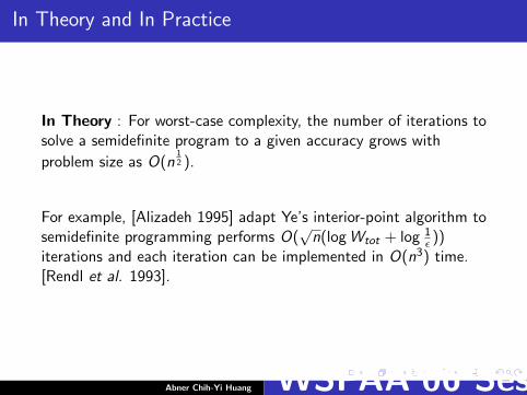
In Theory and In Practice
In Theory : For worst-case complexity, the number of iterations tosolve a semidefinite program to a given accuracy grows with
problem size as O(n12 ).
For example, [Alizadeh 1995] adapt Ye’s interior-point algorithm tosemidefinite programming performs O(
√n(log Wtot + log 1
ε ))iterations and each iteration can be implemented in O(n3) time.[Rendl et al. 1993].
Abner Chih-Yi Huang WSPAA’06 Session 5More on Randomization Semidefinite Programming and Derandomization
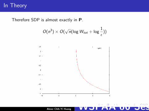
In Theory
Therefore SDP is almost exactly in P.
O(n3)× O(√
n(log Wtot + log1
ε))
Abner Chih-Yi Huang WSPAA’06 Session 5More on Randomization Semidefinite Programming and Derandomization

In Practice
I In Practice : the number of iterations required grows much
more slowly than n12 , perhaps like log(n) or n
14 , and can often
be assumed to be almost constant. (5 to 50 iterations)
It is now generally accepted that interior-point methods for LPs arecompetitive with the simplex method and even faster for problemswith more than 10,000 variables or constraints.[Lustig, et. al.,1994]
Abner Chih-Yi Huang WSPAA’06 Session 5More on Randomization Semidefinite Programming and Derandomization

Conclusion on SDP
From S. Boyd & L. Vandenberghe’s survey paper,
Our final conclusion is therefore: it is not much harder tosolve a rather wide class of nonlinear convex optimizationproblems than it is to solve LPs.
Abner Chih-Yi Huang WSPAA’06 Session 5More on Randomization Semidefinite Programming and Derandomization

The applications of SDP
SDP has applications of control theory, nonlinear programming,geometry, etc. However we might most care the applications oncombinatorial optimization.
I Integer 0/1 Programming problem
I Stable set problem
I Max-cut problem
I Graph coloring problem
I Shannon Capacity of a Graph
I VLSI Layout
...
Abner Chih-Yi Huang WSPAA’06 Session 5More on Randomization Semidefinite Programming and Derandomization
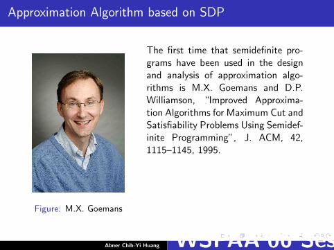
Approximation Algorithm based on SDP
Figure: M.X. Goemans
The first time that semidefinite pro-grams have been used in the designand analysis of approximation algo-rithms is M.X. Goemans and D.P.Williamson, “Improved Approxima-tion Algorithms for Maximum Cut andSatisfiability Problems Using Semidef-inite Programming”, J. ACM, 42,1115–1145, 1995.
Abner Chih-Yi Huang WSPAA’06 Session 5More on Randomization Semidefinite Programming and Derandomization
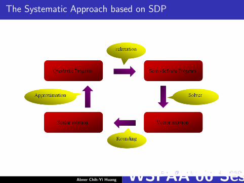
The Systematic Approach based on SDP
Abner Chih-Yi Huang WSPAA’06 Session 5More on Randomization Semidefinite Programming and Derandomization
Why SDP?
In combinatorial optimization, the importance of semidefiniteprogramming is that it leads to tighter relaxations than theclassical linear programming relaxations for many graph andcombinatorial problems.
Abner Chih-Yi Huang WSPAA’06 Session 5More on Randomization Semidefinite Programming and Derandomization
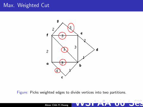
Max. Weighted Cut
Figure: Picks weighted edges to divide vertices into two partitions.
Abner Chih-Yi Huang WSPAA’06 Session 5More on Randomization Semidefinite Programming and Derandomization

Mathematical Programming Expressions for Max.Weighted Cut
Express Max. Weighted Cut problem as integer quadratic programIQP-CUT(x). Edge weight wij = w(vi , vj) if (vi , vj) ∈ E ,wij = 0otherwise.
maximize 12
∑nj=1
∑ji=1 wij(1− yiyj)
subject to yi ∈ {−1, 1} 1 ≤ i ≤ n
Ref. figure 7, nodes a, b
1
2wa,b(1− yayb) =
3
2× (1− (1×−1)) = 3
nodes b, d
1
2wb,d(1− ybyd) =
1
2× (1− (1× 1)) = 0
Abner Chih-Yi Huang WSPAA’06 Session 5More on Randomization Semidefinite Programming and Derandomization

Mathematical Programming Expressions for Max.Weighted Cut
We can relax it to 2-D vector.
maximize 12
∑nj=1
∑ji=1 wij(1−−→yi · −→yj )
subject to −→yi ∈ R2 1 ≤ i ≤ n,−→yi ∈ R2
where −→yi ,−→yj denotes the inner product of vectors, i.e.,
−→yi · −→yj = yi ,1yj ,1 + yi ,2yj ,2.
Abner Chih-Yi Huang WSPAA’06 Session 5More on Randomization Semidefinite Programming and Derandomization
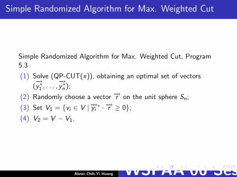
Simple Randomized Algorithm for Max. Weighted Cut
Simple Randomized Algorithm for Max. Weighted Cut, Program5.3
(1) Solve (QP-CUT(x)), obtaining an optimal set of vectors
(−→y∗1 , . . . ,
−→y∗n );
(2) Randomly choose a vector −→r on the unit sphere Sn;
(3) Set V1 = {vi ∈ V | −→yi∗ · −→r ≥ 0};
(4) V2 = V − V1.
Abner Chih-Yi Huang WSPAA’06 Session 5More on Randomization Semidefinite Programming and Derandomization
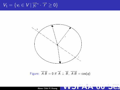
V1 = {vi ∈ V | −→yi∗ · −→r ≥ 0}
Figure:−→A−→B = 0 if
−→A ⊥
−→B ,
−→A−→B = cos(q)
Abner Chih-Yi Huang WSPAA’06 Session 5More on Randomization Semidefinite Programming and Derandomization

Analysis of Algorithm
Denote mRWC (x) be the measure of the solution returned byprogram 5.3. If −→r divide the circle into two sides.
E[mRWC (x)] =n∑
j=1
j∑i=1
wijPr{−→y∗i ,
−→y∗j are in different side}
The probability Pr{−→y∗i ,
−→y∗j are in different side} is the segments of
the circle that−→y∗i ,
−→y∗j dominated.
2cos−1(−→yi
∗ ·−→y∗j )
2π=
cos−1(−→yi∗ ·−→y∗j )
π
(polar-coordinate)
Abner Chih-Yi Huang WSPAA’06 Session 5More on Randomization Semidefinite Programming and Derandomization

V1 = {vi ∈ V | −→yi∗ · −→r ≥ 0}
Figure: Pr{−→y∗i ,
−→y∗j are in different side}
Abner Chih-Yi Huang WSPAA’06 Session 5More on Randomization Semidefinite Programming and Derandomization

Analysis of Algorithm
Compare
E[mRWC (x)] =n∑
j=1
j∑i=1
wij
cos−1(−→yi∗ ·−→y∗j )
π
m∗QP−CUT (x) =
1
2
n∑j=1
j∑i=1
wij(1−−→yi · −→yj )
We have
E[mRWC (x)] =2 cos−1(−→yi
∗ ·−→y∗j )
π(1− cos(cos−1(−→yi∗ ·−→y∗j ))
1
2
n∑j=1
j∑i=1
wij(1−−→yi ·−→yj )
Abner Chih-Yi Huang WSPAA’06 Session 5More on Randomization Semidefinite Programming and Derandomization

Analysis of Algorithm
Let β = min0<α≤π2α
π(1−cos(α) , Since QP-CUT(x) is a relaxation of
IQP-CUT(x), we have
E[mRWC (x)] ≥ β×m∗QP−CUT (x) ≥ β×m∗
IQP−CUT (x) = β×m∗(x)
By Lemma, β > 0.8785. Thus, this algorithm is
1.139-approximation algorithm.
Abner Chih-Yi Huang WSPAA’06 Session 5More on Randomization Semidefinite Programming and Derandomization
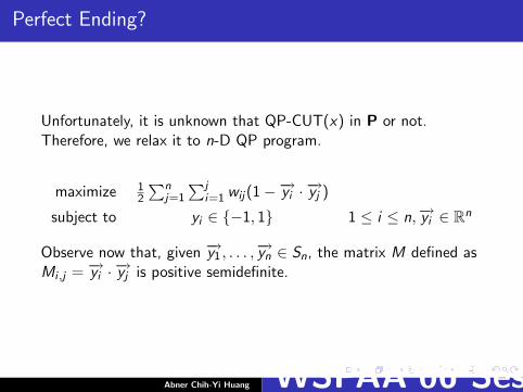
Perfect Ending?
Unfortunately, it is unknown that QP-CUT(x) in P or not.Therefore, we relax it to n-D QP program.
maximize 12
∑nj=1
∑ji=1 wij(1−−→yi · −→yj )
subject to yi ∈ {−1, 1} 1 ≤ i ≤ n,−→yi ∈ Rn
Observe now that, given −→y1 , . . . ,−→yn ∈ Sn, the matrix M defined asMi ,j = −→yi · −→yj is positive semidefinite.
Abner Chih-Yi Huang WSPAA’06 Session 5More on Randomization Semidefinite Programming and Derandomization
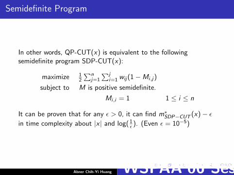
Semidefinite Program
In other words, QP-CUT(x) is equivalent to the followingsemidefinite program SDP-CUT(x):
maximize 12
∑nj=1
∑ji=1 wij(1−Mi ,j)
subject to M is positive semidefinite.
Mi ,i = 1 1 ≤ i ≤ n
It can be proven that for any ε > 0, it can find m∗SDP−CUT (x)− ε
in time complexity about |x | and log(1ε ). (Even ε = 10−5)
Abner Chih-Yi Huang WSPAA’06 Session 5More on Randomization Semidefinite Programming and Derandomization
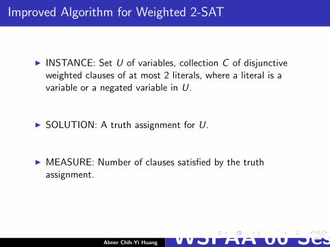
Improved Algorithm for Weighted 2-SAT
I INSTANCE: Set U of variables, collection C of disjunctiveweighted clauses of at most 2 literals, where a literal is avariable or a negated variable in U.
I SOLUTION: A truth assignment for U.
I MEASURE: Number of clauses satisfied by the truthassignment.
Abner Chih-Yi Huang WSPAA’06 Session 5More on Randomization Semidefinite Programming and Derandomization
Improved Algorithm for Weighted 2-SAT
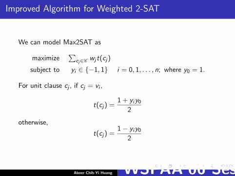
We can model Max2SAT as
maximize∑
cj∈C wj t(cj)
subject to yi ∈ {−1, 1} i = 0, 1, . . . , n; where y0 = 1.
For unit clause cj , if cj = vi ,
t(cj) =1 + yiy0
2
otherwise,
t(cj) =1− yiy0
2
Abner Chih-Yi Huang WSPAA’06 Session 5More on Randomization Semidefinite Programming and Derandomization

Improved Algorithm for Weighted 2-SAT
For example, let c1 = y1, c2 = y2, c3 = y1 + y2, if y1 = 1, y2 = −1,
t(c1) =1 + y1y0
2=
1 + 1× 1
2= 1
and,
t(c2) =1− y2y0
2=
1− (−1× 1)
2= 1
Abner Chih-Yi Huang WSPAA’06 Session 5More on Randomization Semidefinite Programming and Derandomization
Improved Algorithm for Weighted 2-SAT
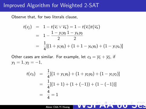
Observe that, for two literals clause,
t(cj) = 1− t(vi ∨ vk) = 1− t(vi )t(vk)
= 1− 1− yiy0
2
1− yky0
2
=1
4[(1 + yiy0) + (1 + 1− yky0) + (1− yiyk)]
Other cases are similar. For example, let c3 = y1 + y2, ify1 = 1, y2 = −1,
t(c3) =1
4[(1 + y1y0) + (1 + y2y0) + (1− y1y2)]
=1
4[(1 + 1) + (1 + (−1)) + (1− (−1))]
=4
4= 1
Abner Chih-Yi Huang WSPAA’06 Session 5More on Randomization Semidefinite Programming and Derandomization

Improved Algorithm for Weighted 2-SAT
It could be expressed as following,
maximize∑n
j=0
∑j−1i=0[aij(1− yiyj) + bij(1 + yiyj)]
subject to yi ∈ {−1, 1} i = 0, 1, · · · , n
where y0 is TRUE, i.e., yi = y0. We can relax it to
maximize∑n
j=0
∑j−1i=0[aij(1− vivj) + bij(1 + vivj)]
subject to vi ∈ Sn vi ∈ V .
Abner Chih-Yi Huang WSPAA’06 Session 5More on Randomization Semidefinite Programming and Derandomization
Improved Algorithm for Weighted 2-SAT
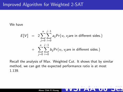
We have
E [V ] = 2n∑
j=0
j−1∑i=0
aijPr{vi , vjare in different sides.}
+n∑
j=0
j−1∑i=0
bijPr{vi , vjare in different sides.}
Recall the analysis of Max. Weighted Cut. It shows that by similarmethod, we can get the expected performance ratio is at most1.139.
Abner Chih-Yi Huang WSPAA’06 Session 5More on Randomization Semidefinite Programming and Derandomization
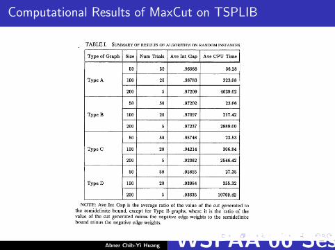
Computational Results of MaxCut on TSPLIB
Abner Chih-Yi Huang WSPAA’06 Session 5More on Randomization Semidefinite Programming and Derandomization

More Computational Results
[Homer, et. al., 1997] have implemented our algorithm on a CM-5,and have shown that it produces optimal or very nearly optimalsolutions to a number of MAX CUT instances derived from viaminimization problems.
Abner Chih-Yi Huang WSPAA’06 Session 5More on Randomization Semidefinite Programming and Derandomization
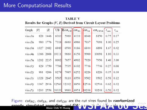
More Computational Results
Figure: cutRG , cutSA, and cutGW are the cut sizes found by randomizedgreedy, simulated annealing, and GW respectively. The column tconv
displays the time spent to find a near optimal vector configuration.Abner Chih-Yi Huang WSPAA’06 Session 5More on Randomization Semidefinite Programming and Derandomization

More Computational Results
I The results for simulated annealing are the best cuts foundover 5 runs of 107 annealing steps each.
I The results for randomized greedy are the maximum cutsfound over 20, 000 independent runs.
I Column UB displays the upper bounds which were derivedfrom the dual solutions. Our corresponding primal and dualapproximations of the optimum are within 0.05% of eachother and therefore within 0.05% of the true upper bound.
Abner Chih-Yi Huang WSPAA’06 Session 5More on Randomization Semidefinite Programming and Derandomization
Bibliography I
I G. Ausiello, P. Crescenzi, G. Gambosi, V. Kann, A.Marchetti-Spaccamela, M. Protasi (1999) Complexity andApproximation, Springer Verlag.
I Kabanets, V. Derandomization: A Brief Overview ElectronicColloquium on Computational Complexity, 2002, 9.
I Mahajan, S. & Ramesh, H. Derandomizing ApproximationAlgorithms Based on Semidefinite Programming SIAM J.Comput., Society for Industrial and Applied Mathematics,1999, 28, 1641-1663
I Impagliazzo, R. Hardness as randomness: a survey of universalderandomization Proceedings of the ICM, Beijing 2002, 2002,3, 659-672
Abner Chih-Yi Huang WSPAA’06 Session 5More on Randomization Semidefinite Programming and Derandomization
Bibliography II
I Goemans, M.X. & Williamson, D.P. Improved approximationalgorithms for maximum cut and satisfiability problems usingsemidefinite programming J. ACM, ACM Press, 1995, 42,1115-1145.
I Y. Nesterov and A. Nemirovskii. Self-Concordant Functionsand Polynomial Time Methods in Convex Programming.Central Economic and Mathematical Institute, USSRAcademy of Science, .Moscow, 1989.
I F. Alizadeh, ”Interior Point Methods in SemidefiniteProgramming with Applications to CombinatorialOptimization”, SIAM J. Optim., vol 5, No. 1, pp. 13–51,1995 RENDL, F., VANDERBEI, R., AND WOLKOWICZ, H.1993. Interior point methods for max-min eigenvalueproblems. Report 264, Technische Universitat Graz, Graz,Austria.
Abner Chih-Yi Huang WSPAA’06 Session 5More on Randomization Semidefinite Programming and Derandomization

Bibliography III
I Vandenberghe, L. & Boyd, S. Semidefinite programmingSIAM Review, 1996, 38, 49-95
I S. Boyd and L. Vandenberghe, Convex Optimization.Cambridge University Press, 2003.
I Lecture Notes of Randomized Algorithms, Prof. Hsueh-I Lu.
I Rajeev Motwani, Prabhakar Raghavan , RandomizedAlgorithms, Cambridge University Press, August 25, 1995.
I I. J. Lustig, R. E. Marsten, and D. F. Shanno, Interior pointmethods for linear programming: Computational state of theart, ORSA Journal on Computing, 6, 1994
I Steven Homer and Marcus Peinado, Design and Performanceof Parallel and Distributed Approximation Algorithms forMaxcut, Journal of Parallel and Distributed Computing,Volume 46, Issue 1, , 10 October 1997, Pages 48-61.
Abner Chih-Yi Huang WSPAA’06 Session 5More on Randomization Semidefinite Programming and Derandomization
Session 5: More on Randomization
End! Thanks!
Abner Chih-Yi Huang WSPAA’06 Session 5More on Randomization Semidefinite Programming and Derandomization