more accurate pressure solves. solid boundaries voxelized version works great if solids aligned...
Post on 19-Dec-2015
215 views
TRANSCRIPT
More Accurate Pressure Solves
Solid Boundaries
Voxelized version works great if solids aligned with grid
If not: though the error in geometry is O(∆x), translates into O(1) error in velocities!
The simulation physics sees stair-steps, and gives you motion for the stair-step case
Quick Fix
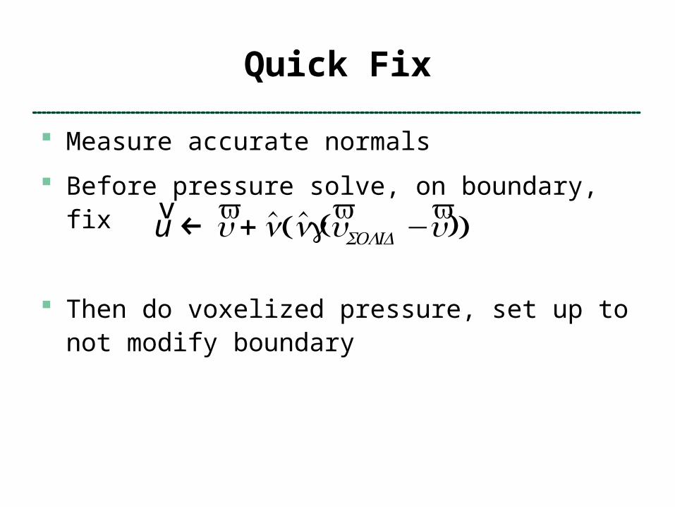
Measure accurate normals
Before pressure solve, on boundary, fix
Then do voxelized pressure, set up to not modify boundary
vu ← vu+ n ng(vuSOLID −vu)( )
Quick Fix Fails
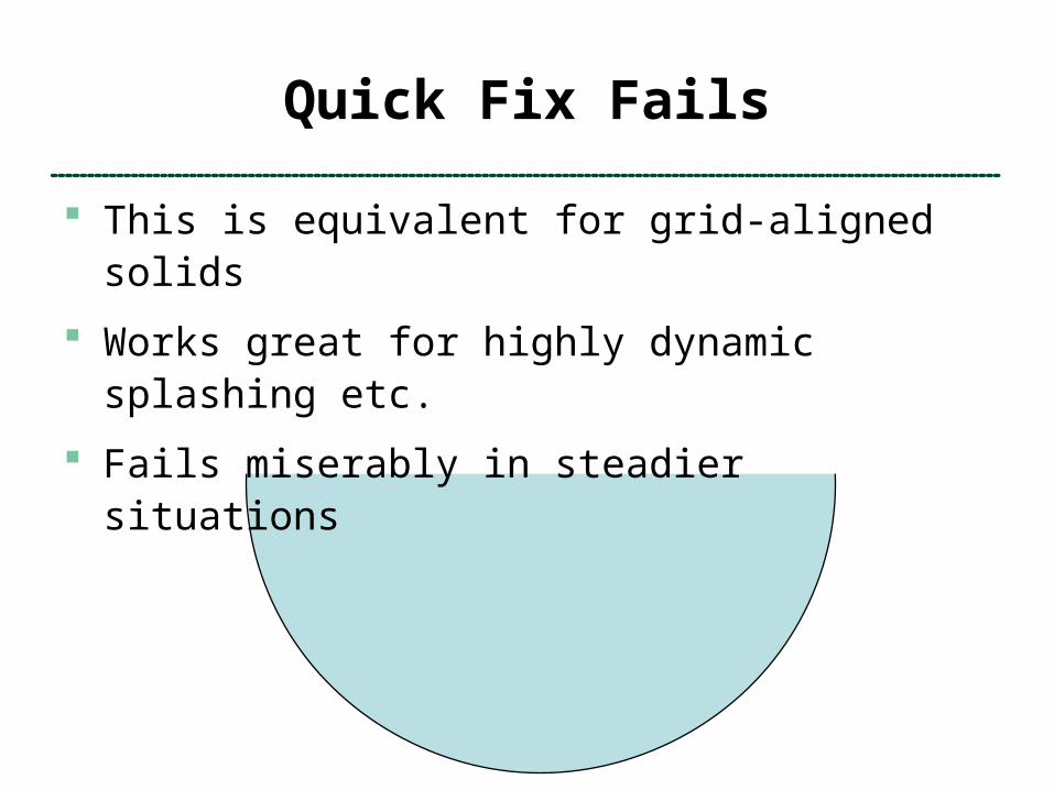
This is equivalent for grid-aligned solids
Works great for highly dynamic splashing etc.
Fails miserably in steadier situations
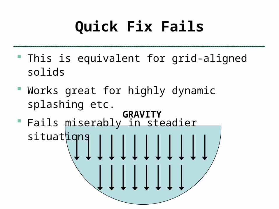
Quick Fix Fails
This is equivalent for grid-aligned solids
Works great for highly dynamic splashing etc.
Fails miserably in steadier situationsGRAVITY
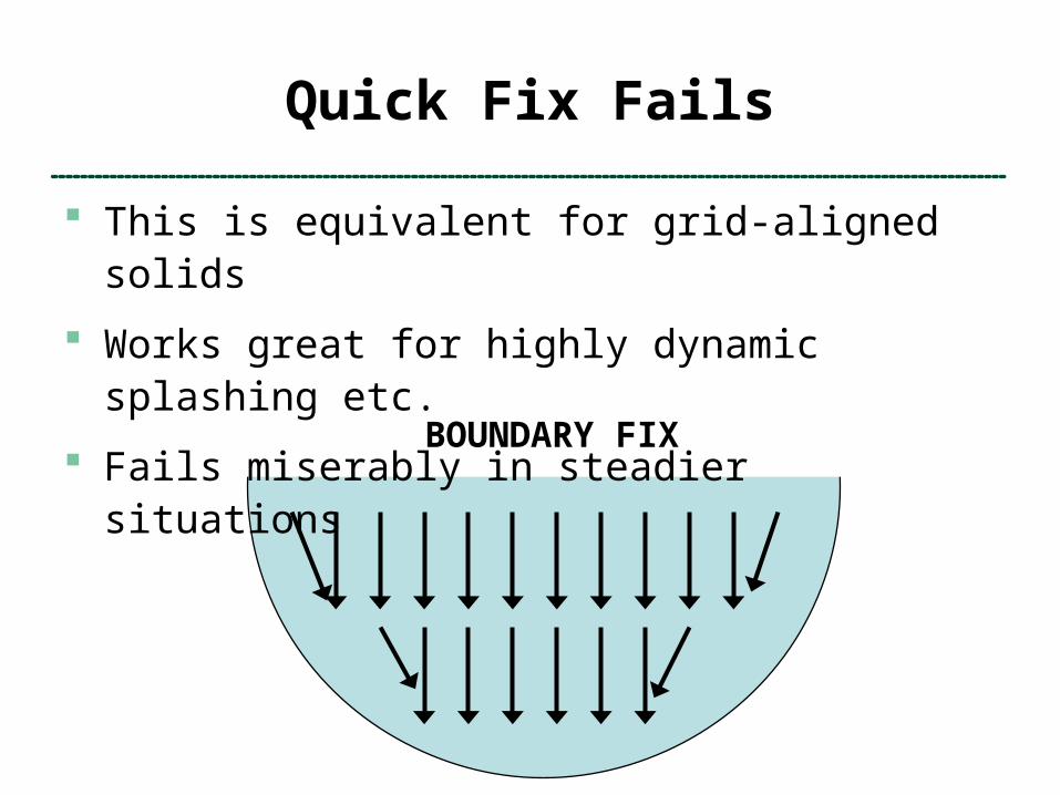
Quick Fix Fails
This is equivalent for grid-aligned solids
Works great for highly dynamic splashing etc.
Fails miserably in steadier situationsBOUNDARY FIX

Quick Fix Fails
This is equivalent for grid-aligned solids
Works great for highly dynamic splashing etc.
Fails miserably in steadier situationsPRESSURE SOLVE
Quick Fix Fails
This is equivalent for grid-aligned solids
Works great for highly dynamic splashing etc.
Fails miserably in steadier situations
Fictitious currents emerge and unstably grow
Rethinking the problem
See Batty et al. (tomorrow)
If we keep our fluid blobs constant volume, incompressibility constraint means:blobs stay in contact with each other (no interpenetration, no gaps)
Staying in contact == inelastic, sticky collision
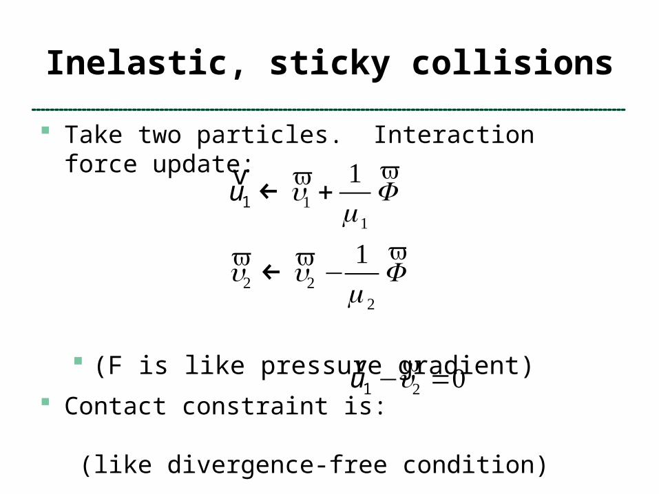
Inelastic, sticky collisions
Take two particles. Interaction force update:
(F is like pressure gradient) Contact constraint is:
(like divergence-free condition)
vu1 ←
vu1 +1m1
vF
vu2 ← vu2 −1m2
vF
vu1 −
vu2 =0
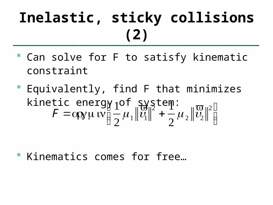
Inelastic, sticky collisions (2)
Can solve for F to satisfy kinematic constraint
Equivalently, find F that minimizes kinetic energy of system:
Kinematics comes for free…
F =argmin
12
m1vu1
2 +12
m2vu2
2⎛⎝⎜
⎞⎠⎟
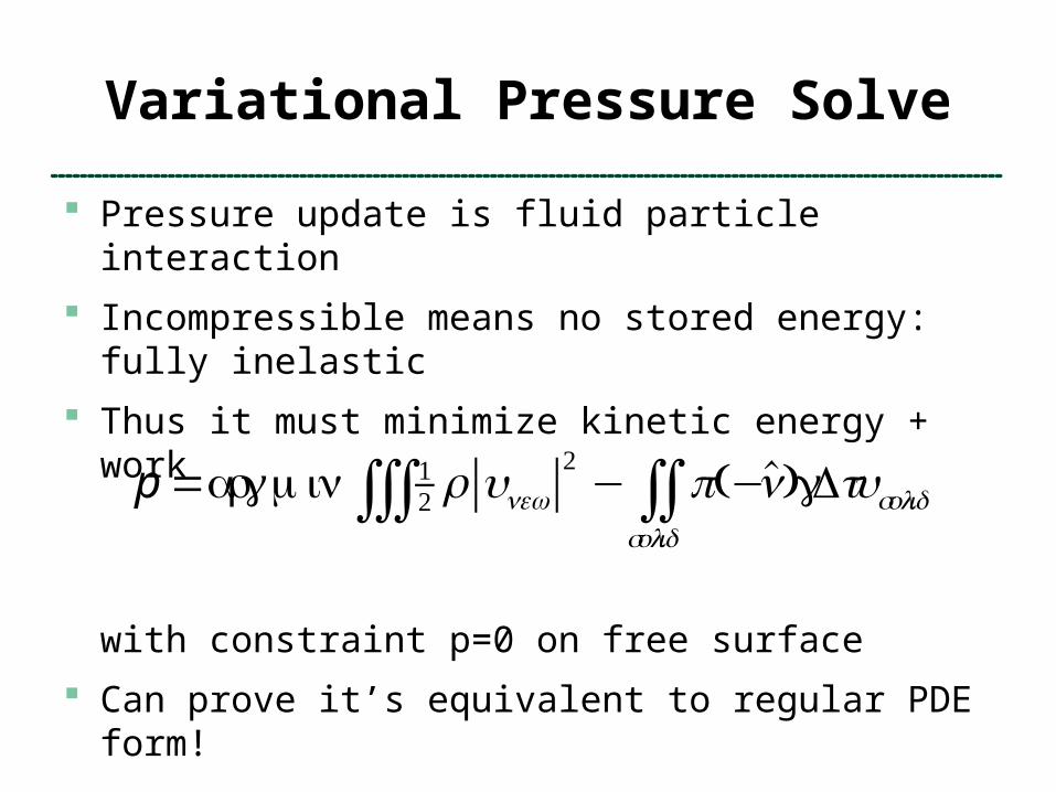
Variational Pressure Solve
Pressure update is fluid particle interaction
Incompressible means no stored energy:fully inelastic
Thus it must minimize kinetic energy + work
with constraint p=0 on free surface
Can prove it’s equivalent to regular PDE form!
p =argmin 1
2 ρ unew2
∫∫∫ − p(−n)gΔtusolidsolid∫∫
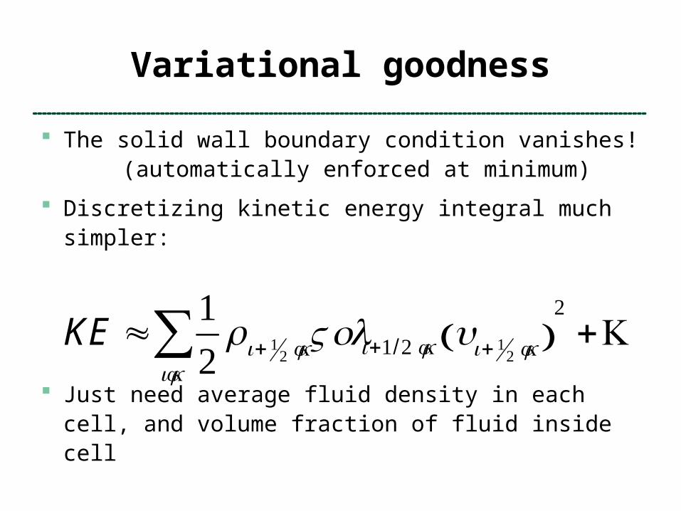
Variational goodness
The solid wall boundary condition vanishes!(automatically enforced at minimum)
Discretizing kinetic energy integral much simpler:
Just need average fluid density in each cell, and volume fraction of fluid inside cell
KE ≈
12ρi+ 1
2 jkVoli+1/2 jk ui+ 12 jk( )
2
ijk∑ +K
Linear System
Plug in discrete pressure update in discrete KE
Quadratic in pressures
Find discrete minimum == solve linear system
Linear system guaranteed to be symmetric, positive definite
In fact, it’s exactly the same as voxelized– except each term is weighted by volume fractions
Benefits
Actually converges! (error is O(∆x) or better)
Handles resting case perfectly:KE is minimized by zeroing out velocity, which we get from hydrostatic pressure field
Can handle sub-grid-scale geometry
E.g. particles immersed in flow, narrow channels, hair…
Just need to know volume displaced!
Extra goodness
Can couple solids in flow easily:
Figure out formula for discrete pressure update to solid velocity
Add solid’s kinetic energy to minimization
Automatically gives two-way “strong” coupling between rigid bodies and flow, perfectly compatible velocities at boundary, no tangential coupling…

Free Surfaces
The other problem we see with voxelization is free surface treatment
Physics only sees voxels: waves less than O(∆x) high are ignored
At least position errors will converge to zero… but errors in normal are O(1)!(rendering will always look awful)

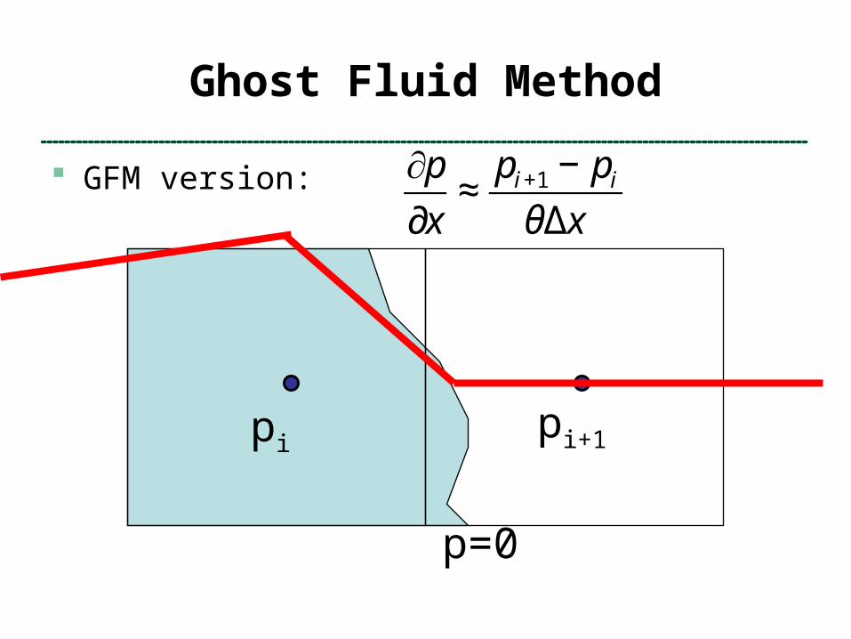
Ghost Fluid Method
Due to Fedkiw and coauthors
pi pi+1
p=0

Ghost Fluid Method
Voxelized version:
pi pi+1
p=0
∂p∂x≈pi+1 − piΔx
Ghost Fluid Method
GFM version:
pi pi+1
p=0
∂p∂x≈pi+1 − piθΔx
GFM with solids
Complementary to variational solve:GFM just changes the pressure update
However, for triple junctions (solid+liquid+air) it gets difficult to make this just right
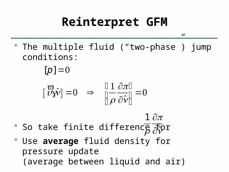
Reinterpret GFM
The multiple fluid (“two-phase”) jump conditions:
So take finite difference for
Use average fluid density for pressure update(average between liquid and air)
[p]=0
vugn[ ] =0 ⇒1ρ
∂p∂n
⎡
⎣⎢
⎤
⎦⎥=0
1
ρ∂p∂n

Variational free surface
Simply need volume fractions per cell(how much of cell is liquid+air),and average densities per cell(mix between liquid and air)
Use average density for pressure update, volume fraction for KE estime
Speed things up: all-air cells eliminated(set p=0 there)
This is the discrete free surface approximation!