More about Spark

Mirek Riedewald

This work is licensed under the Creative Commons Attribution 4.0 International License. To view a copy of this license, visit http://creativecommons.org/licenses/by/4.0/.

Key Learning Goals• What is the purpose of Spark SQL, Spark

Streaming, Spark MLlib, and Spark GraphX?• Why do map and flatMap remove the Partitioner

of a pair RDD? Why do mapValues and flatMapValues preserve the Partitioner of a pair RDD?

• When can the hash+shuffle join on pair RDDs avoid shuffling?

• Given a Spark program, determine how many jobs are going to be executed.

• Given a Spark program, determine which operations are executed by the master and which by the worker tasks.

2

Introduction

• This module surveys important components and aspects of Spark that have not been covered in detail yet:

– Spark SQL

– Spark Streaming

– Spark MLlib

– Spark GraphX

– Partitioning and shuffling in Spark

– The interplay between lineage, jobs and lazy execution.

3

4

Let us start with SQL operations in Spark.

SQL Basics• SQL is based on the relational calculus. A calculus

expression describes what we are looking for, not how to compute it.

• The computation steps and their order of execution are expressed in relational algebra. For a given SQL query, the logical query plan corresponds to an expression in relational algebra.

• Relational algebra has only 5 primitive operators, which can be combined to compose complex queries: selection, projection, Cartesian product (a.k.a. cross product or cross join), set union, and set difference.– The renaming operator is needed for formal reasons but does

not manipulate data.

• In addition, grouping and aggregation operators were introduced as well. We already encountered most of these operators before.

5

Reminder: Selection and Projection

6

DBMS (SQL): Assume the input relation R has schema (A1, A2, A3); P is a predicate returning true/false; F is a function

Selection: SELECT * FROM R WHERE F(A1, A2, A3)Projection (on A1): SELECT A1 FROM RExtended projection: SELECT F(A1, A2, A3) FROM R

Spark:

myRDD.filter( P(x) ) // selectionmyRDD.map( x => F(x) ) // extended projection

myDS.filter( P(x) ) // selectionmyDS.select( “A1” ) // projectionmyDS.map( x => F(x) ) // extended projection

Reminder: Grouping and Aggregation

7

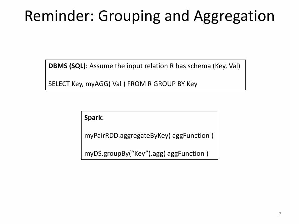
DBMS (SQL): Assume the input relation R has schema (Key, Val)

SELECT Key, myAGG( Val ) FROM R GROUP BY Key

Spark:

myPairRDD.aggregateByKey( aggFunction )

myDS.groupBy(“Key”).agg( aggFunction )

Cartesian Product

8

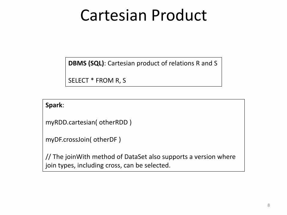
DBMS (SQL): Cartesian product of relations R and S

SELECT * FROM R, S

Spark:

myRDD.cartesian( otherRDD )

myDF.crossJoin( otherDF )

// The joinWith method of DataSet also supports a version where join types, including cross, can be selected.

Set Difference• Set functions generally require both inputs to be of the

same type.• rdd1.subtract(rdd2) transformation: returns all

elements from rdd1 that are not in rdd2. This is for ordinary RDDs and hence compares the entire element.

• rdd1.subtractByKey(rdd2) transformation: This is for pair RDDs, returning all elements from rdd1 whose keys do not appear as key in rdd2.

• For DataSet, the corresponding transformation is except.– Equality checking is performed directly on the encoded

representation of the data and thus is not affected by a custom equals function defined on the element type.

9

Union and Intersection in Spark

• rdd1.union(rdd2) transformation: returns all elements that occur in either input, but does not remove duplicates.

– For DataSet, the corresponding functions are unionand unionByName.

• rdd1.intersection(rdd2) transformation: returns all elements that occur in both.

– For DataSet, the corresponding function is intersect.

• Intersection does not add new functionality—it can be expressed with union and set difference.

10

Reminder: Joins

• The join can be expressed as a selection applied to the Cartesian product. Then why was it introduced as a separate operator?

– Joins are very common in practice, and they tend to be expensive to compute. Since most joins in databases are equi-joins, specialized techniques were proposed to reduce their computation cost.

• Refer to the module on joins for Spark join operations.

11

Zip—A Special Join• rdd1.zip(rdd2) transformation: for rdd1 of type T and rdd2 of type

U, it returns pairs of type (T, U), where the i-th pair consists of the i-th records from rdd1 and from rdd2.– Both RDDs must have the same number of partitions and elements in

them.– The zipPartitions transformation is similar, but more flexible in zipping

even partitions with different numbers of elements.

• When is this useful? Consider computation of PageRank. Conceptually we are dealing with two data sets: the graph and the PageRank values. The former is read repeatedly, while the latter changes in each iteration. Hence we want to store the graph as a pair RDD (pageID, adjacencyList) and the PageRank values as (pageID, PRvalue). To compute outgoing contributions for a page N, both N’s adjacency list and current PR value are needed. Using zip to combine the values is more efficient (and elegant) than using a join or trying a workaround with intersection. We just have to make sure that there really is a one-to-one correspondence between records in both data sets.

12

Spark SQL• Spark SQL works with DataFrames.

– Reminder: A DataFrame is like a database table. It consists of rows, each adhering to a fixed schema that defines the name and type of all columns. You can think of a DataFrame as an RDD with additional structure. In recent Spark versions, it is an alias for DataSet[Row].

• DataFrames can be processed using SQL and SQL-inspired functions. Think of Spark SQL as a distributed Spark-powered SQL query processor. It can even be accessed like a database server using JDBC.

• Operations on DataFrames are translated into optimized low-level RDD operations. Like in a DBMS, the structure enables optimizations not possible for general RDDs.

13

Implementation Notes

• Spark’s default file format for structured data is Parquet.

• DataFrame metadata is managed in a table catalog. Spark applications can then access a DataFrame by name.

– This information disappears when the Spark context is restarted. To make the catalog persistent, Spark needs to be built with Hive support.

14

Creating and Storing DataFrames• DataFrames can be created as follows:

– Convert an RDD.– Run an SQL query.– Load external data.

• Spark can easily load and import data from JDBC sources, Hive, and files in JSON, ORC, and Parquet format.

• Parquet organizes the DataFrame column-wise, using compression. By saving the min and max value for each column chunk, some queries can skip chunks.– For example, consider a query computing average income

for people of age 30 to 40. A chunk with min age 55 and max age 69 is completely irrelevant, but a chunk covering range 37 to 62 would have to be accessed.

15

Working with DataFrames

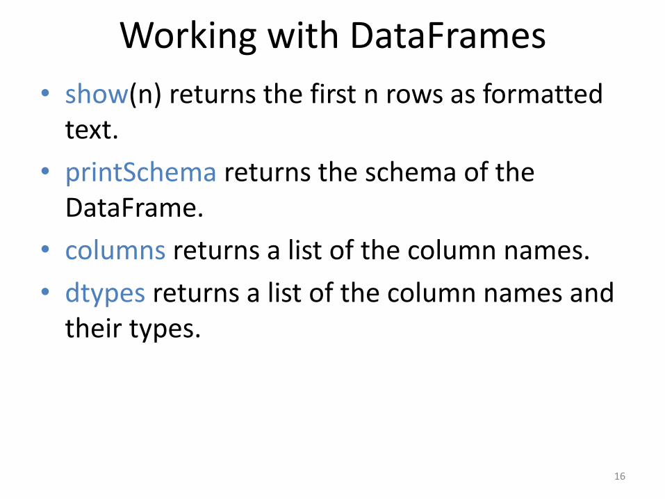
• show(n) returns the first n rows as formatted text.

• printSchema returns the schema of the DataFrame.

• columns returns a list of the column names.

• dtypes returns a list of the column names and their types.

16

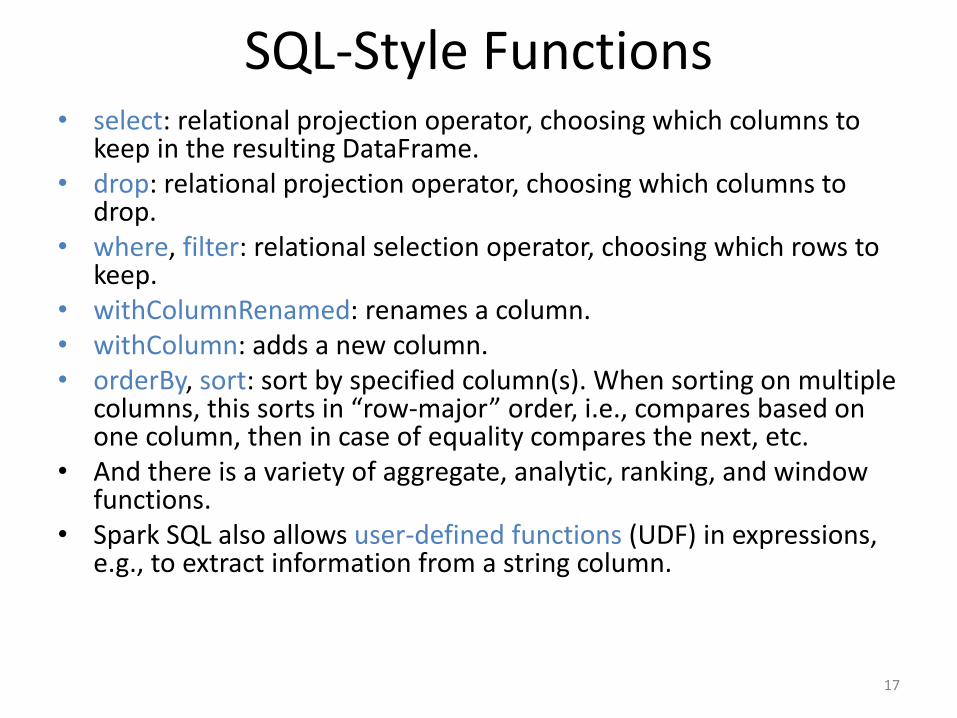
SQL-Style Functions• select: relational projection operator, choosing which columns to

keep in the resulting DataFrame.• drop: relational projection operator, choosing which columns to

drop.• where, filter: relational selection operator, choosing which rows to

keep.• withColumnRenamed: renames a column.• withColumn: adds a new column.• orderBy, sort: sort by specified column(s). When sorting on multiple

columns, this sorts in “row-major” order, i.e., compares based on one column, then in case of equality compares the next, etc.

• And there is a variety of aggregate, analytic, ranking, and window functions.

• Spark SQL also allows user-defined functions (UDF) in expressions, e.g., to extract information from a string column.

17

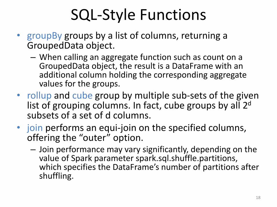
SQL-Style Functions• groupBy groups by a list of columns, returning a

GroupedData object.– When calling an aggregate function such as count on a

GroupedData object, the result is a DataFrame with an additional column holding the corresponding aggregate values for the groups.

• rollup and cube group by multiple sub-sets of the given list of grouping columns. In fact, cube groups by all 2d

subsets of a set of d columns.• join performs an equi-join on the specified columns,

offering the “outer” option.– Join performance may vary significantly, depending on the

value of Spark parameter spark.sql.shuffle.partitions, which specifies the DataFrame’s number of partitions after shuffling.

18

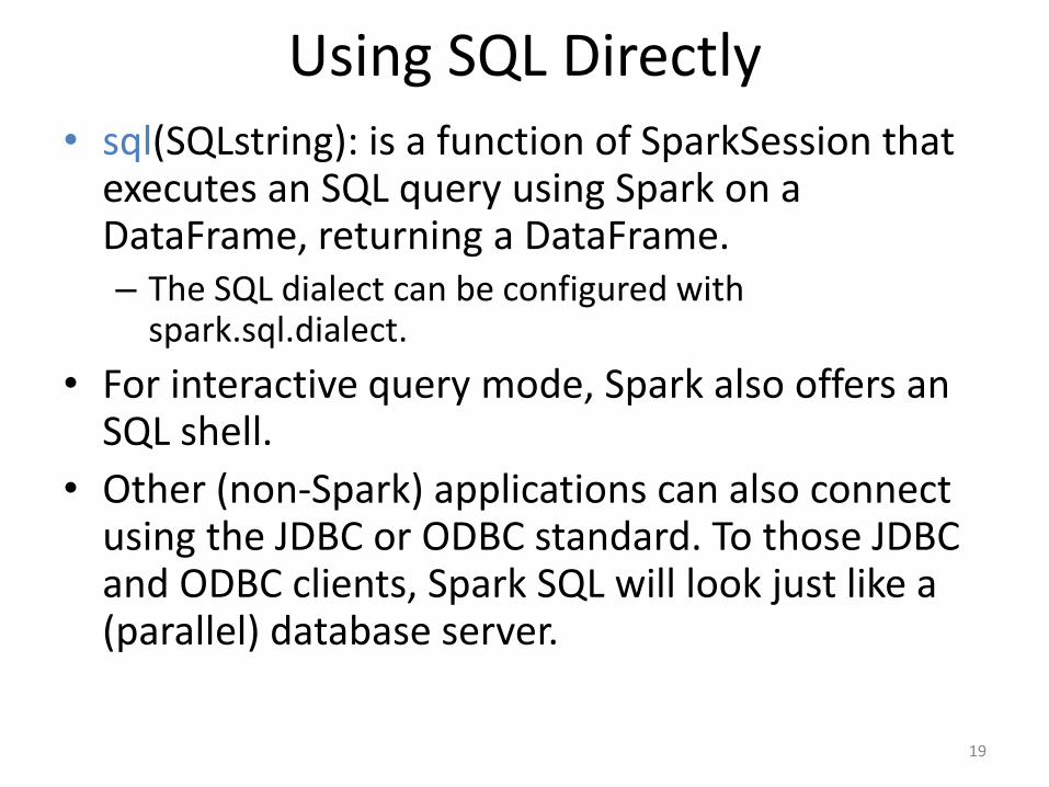
Using SQL Directly• sql(SQLstring): is a function of SparkSession that

executes an SQL query using Spark on a DataFrame, returning a DataFrame.– The SQL dialect can be configured with

spark.sql.dialect.

• For interactive query mode, Spark also offers an SQL shell.

• Other (non-Spark) applications can also connect using the JDBC or ODBC standard. To those JDBC and ODBC clients, Spark SQL will look just like a (parallel) database server.

19

Query Optimization• Like in a DBMS, Spark’s Catalyst optimizer translates a

query into Spark jobs. It goes through several steps:– The query is parsed and relation references are checked to

produce the logical plan.– This plan is optimized, mostly by re-arranging (e.g., projection

and filter before join) and combining (e.g., apply multiple filters on same relation together) operations. It currently is based on “safe” heuristics but could be extended to include cost estimation.

– From the optimized logical plan, a physical plan is generated, which includes operator implementation choices. Here cost models should be used to decide between different join implementations.

– Finally, the physical plan is translated into Spark jobs.

• To see the logical and physical plans, use DataFrame’sexplain method. They can also be seen through the Web UI.

20

21

We next take a quick look at Spark Streaming.

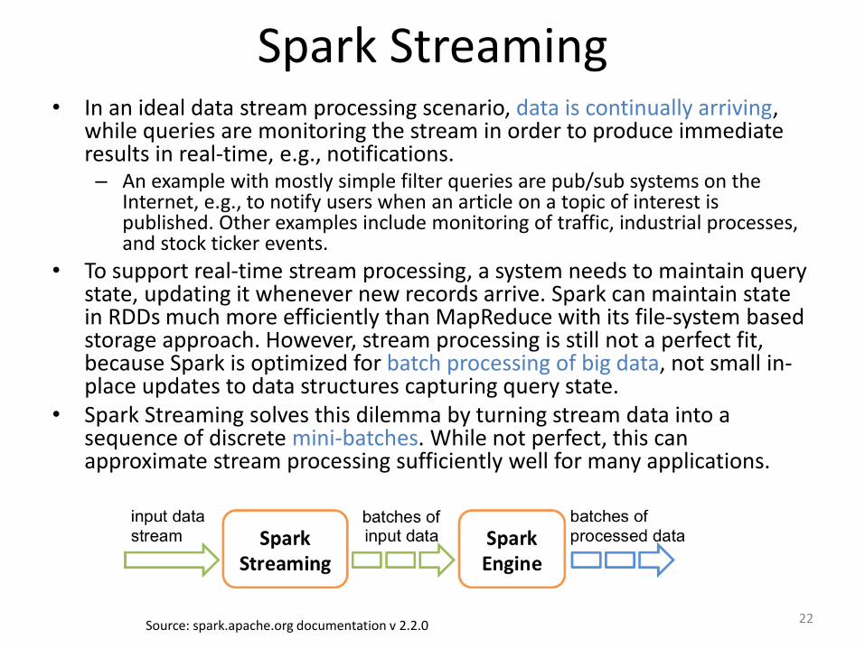
Spark Streaming• In an ideal data stream processing scenario, data is continually arriving,

while queries are monitoring the stream in order to produce immediate results in real-time, e.g., notifications.– An example with mostly simple filter queries are pub/sub systems on the

Internet, e.g., to notify users when an article on a topic of interest is published. Other examples include monitoring of traffic, industrial processes, and stock ticker events.

• To support real-time stream processing, a system needs to maintain query state, updating it whenever new records arrive. Spark can maintain state in RDDs much more efficiently than MapReduce with its file-system based storage approach. However, stream processing is still not a perfect fit, because Spark is optimized for batch processing of big data, not small in-place updates to data structures capturing query state.

• Spark Streaming solves this dilemma by turning stream data into a sequence of discrete mini-batches. While not perfect, this can approximate stream processing sufficiently well for many applications.

22Source: spark.apache.org documentation v 2.2.0

Reading Streaming Data• Using the appropriate receiver, Spark Streaming

can read data from file systems such as HDFS and S3, from TCP/IP sockets, and from distributed systems such as Twitter, Flume, and Kafka.

• Each incoming mini-batch is represented by an RDD. Hence the full power of Spark can be applied to combine existing RDDs in memory with the new mini-batch RDD.– When reading from a file system, a mini-batch consists

of all the newly created files, since the last batch, in the input folder. Data added to existing files will not be included!

23

Working with Streams• There are several features in addition to the usual Spark

operations.• The DStream class represents the discretized stream,

supporting basic operations such as map, filter, and window.

• For DStreams of key-value pairs, additional functions such as groupByKeyAndWindow and join exist.– updateStateByKey updates the state of each key, by applying a

supplied function to the old state and newly arriving values for the key.

– mapWithState generalizes updateStateByKey and can maintain state of some type, while returning data of another. It also apparently can manage larger state (more keys) and is significantly faster than updateStateByKey.

• DStream operations are executed automatically by the streaming context once per new mini-batch.

24

Mini-Batch Management

25Source: spark.apache.org documentation v 2.2.0

Window-Based Processing• Conceptually, a data stream is infinite. Hence some operations

cannot be applied to it, e.g., sorting.– We can never output any result, because in the next moment a

smaller value might arrive.

• For other operations, state would grow without bounds, e.g., join. By defining windows of bounded length, these problems go away.

• Windows are also useful as a query feature in their own right, e.g., to determine the most active customer in each month or the most active user in the last hour.

• In Spark, windows are defined based on duration and slide, which must be multiples of the DStream’s batch interval. (This way each window corresponds to an integer number of mini-batches.)– Consider a batch interval of 5 sec, duration of 20 sec and slide of 10

sec. The first window then consists of mini-batches (0, 1, 2, 3), the next of (2, 3, 4, 5), then (4, 5, 6, 7), and so on. Note how the slide parameter results in “jumping” for the first mini-batch in the window.

26

Performance Considerations• A smaller batch interval (i.e., mini-batch duration) is better for more

timely response to incoming data. However, it must be large enough, so that all processing of a mini-batch completes within the interval. Note that larger batches tend to reduce per-record processing cost.– More formally, a smaller interval is better for low latency, while a

larger interval is better for high throughput.

• We can use the Web UI to see if the system can keep up with the arriving mini-batches.

• Since application state depends on a conceptually infinite stream, it is infeasible to recompute it when a failure happens.– Executor failure: Data replication enables recovery of failed executors

on a different machine.– Driver failure: Checkpointing of the entire streaming application

enables quick recovery by restarting the driver and reading the checkpointed data.

27

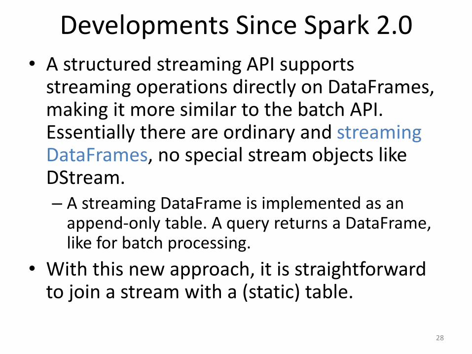
Developments Since Spark 2.0

• A structured streaming API supports streaming operations directly on DataFrames, making it more similar to the batch API. Essentially there are ordinary and streaming DataFrames, no special stream objects like DStream.– A streaming DataFrame is implemented as an

append-only table. A query returns a DataFrame, like for batch processing.

• With this new approach, it is straightforward to join a stream with a (static) table.

28

29

We introduced some functionality of Spark MLlib in earlier modules. Here we briefly survey additional functionality.

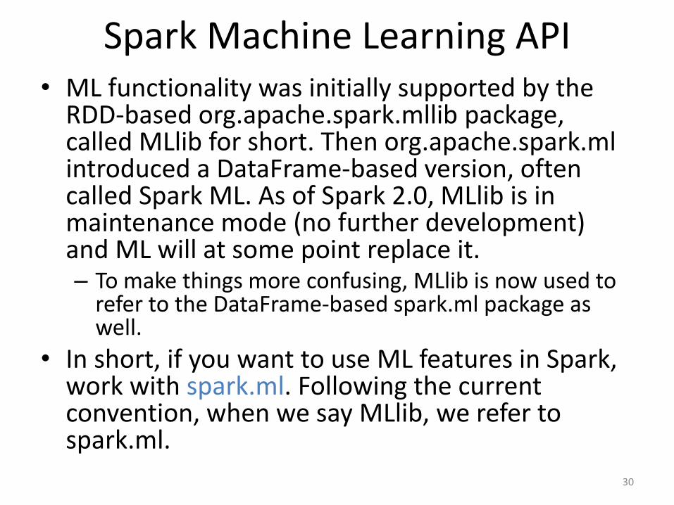
Spark Machine Learning API• ML functionality was initially supported by the

RDD-based org.apache.spark.mllib package, called MLlib for short. Then org.apache.spark.ml introduced a DataFrame-based version, often called Spark ML. As of Spark 2.0, MLlib is in maintenance mode (no further development) and ML will at some point replace it.– To make things more confusing, MLlib is now used to

refer to the DataFrame-based spark.ml package as well.

• In short, if you want to use ML features in Spark, work with spark.ml. Following the current convention, when we say MLlib, we refer to spark.ml.

30

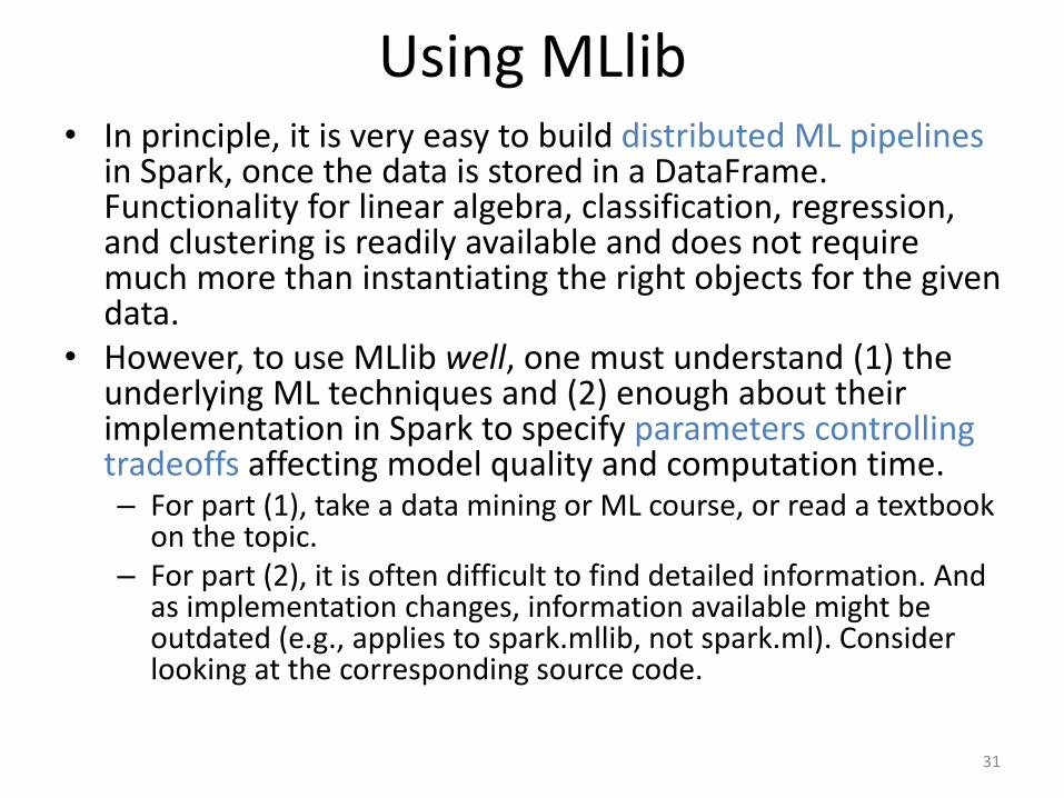
Using MLlib• In principle, it is very easy to build distributed ML pipelines

in Spark, once the data is stored in a DataFrame. Functionality for linear algebra, classification, regression, and clustering is readily available and does not require much more than instantiating the right objects for the given data.

• However, to use MLlib well, one must understand (1) the underlying ML techniques and (2) enough about their implementation in Spark to specify parameters controlling tradeoffs affecting model quality and computation time.– For part (1), take a data mining or ML course, or read a textbook

on the topic.– For part (2), it is often difficult to find detailed information. And

as implementation changes, information available might be outdated (e.g., applies to spark.mllib, not spark.ml). Consider looking at the corresponding source code.

31

Important Functionality• ml.clustering offers a variety of clustering techniques,

including K-means, Latent Dirchlet Allocation (LDA), and Gaussian Mixture Model (GMM).

• ml.classification offers a variety of models for predicting nominal outcomes (e.g., if a credit card transaction is fraudulent or not) that can be trained on labeled data. This includes RandomForest, gradient-boosted tree, decision tree, logistic regression, artificial neural network (multilayer perceptron), and Naïve Bayes.

• ml.regression offers models for predicting numerical outcomes (e.g., income) from labeled data. This includes RandomForest, gradient-boosted tree, decision tree, and (generalized) linear regression.

32

Important Functionality• Model evaluation methods are in ml.evaluation.

• ml.linalg supports both dense and sparse linear algebra operations, including matrix product and transpose.

• ml.attribute supports functionality to represent the given data.

• ml.feature offers a variety of pre-processing and data manipulation techniques, commonly used for ML tasks. This includes feature scaling, normalization, PCA, inverse document frequency (IDF), string indexing, and Word2Vec.

• For classification and regression, cross-validation and training/test splitting functionality can be found in ml.tuning.

33

Random Forest Implementation Notes• How is training for Random Forest implemented in Spark? One

could partition work at the granularity of trees; or one could even parallelize training of a tree itself.

• To support cases with many machines and few trees, Spark implemented the more fine-grained version based on Google research paper [Biswanath Panda and Joshua S. Herbach and Sugato Basu and Roberto J. Bayardo. PLANET: Massively Parallel Learning of Tree Ensembles with MapReduce. Proc. Int. Conf. on Very Large Data Bases (VLDB), 2009].– As an artifact of this training approach, the maxBins parameter

controls training cost versus split quality based on the number of split candidates considered for continuous features.

• The trained model is returned to the driver and stored there in memory. For large data with many trees in the ensemble, this may create a memory bottleneck.– A possible workaround would be to implement the ensemble as a set

of decision trees, e.g., to explicitly manage the set of trees in an RDD in user code.

34

Random Forest Parameters• Random Forest and Bagged tree ensembles require little parameter tuning

and tend to produce excellent predictions. We recommend the following default parameter settings:– Set numTrees high, e.g., to 100. Or start with few trees and then increase the

number until model quality reaches a ceiling.– Do not limit maxDepth, which limits tree height. In practice, splits tend to

distribute data unevenly between branches. Hence the number of records in different nodes at the same level can vary by orders of magnitude.

– Set minInstancesPerNode = 50 for binary classification and regression; larger for multi-class problems. This ensures each leaf has enough data to capture the fraction of the majority class (classification) or the output average (regression) “reasonably” well. And it lets branches with more data grow deeper. Unfortunately, it might generate overly small trees in the presence of multi-way splits (on categorical attributes).• Consider a tree node with 10M records, where the best split is on a categorical attribute

resulting in a partitioning of size (4M, 3M, 3M-1, 1). Typically, it is beneficial to split such a node, but unless minInstancesPerNode = 1, this split would be prevented because of the branch receiving one record.

– A better solution would be a parameter that stops splitting not based on childbranches but based on the number of records in the node to be split.

– As a workaround, one could convert a categorical attribute with n possible values to n different binary attributes (aka one-hot encoding).

35

36

Next we take a quick look at the GraphXlibrary for graph analysis.

GraphX• The GraphX package supports graph representation as

RDDs and a variety of important graph algorithms, including (strongly) connected components, label propagation for community detection, PageRank, shortest path, and triangle count.

• Furthermore, efforts are being undertaken to support the behavior of other popular graph analysis frameworks on top of GraphX. For example, the Pregel object in spark.graphx supports an interface similar to Google’s Pregel, with GraphX providing a highly efficient implementation.

• As with MLlib, using existing GraphX algorithms, e.g., PageRank, is easy, but one has to trust that the provided implementation is efficient. Finding implementation details is difficult. For instance, can you find out how the provided PageRank algorithm handles dangling nodes?

37

Implementing A Graph Algorithm• When implementing your own graph algorithm in GraphX,

intelligent caching is particularly important.• Many graph algorithms proceed in rounds, reading graph structure

such as a node’s adjacency list, in each round. It therefore often pays off to have the graph cached, using the cache() or persist()method.

• Other graph information changes in each round, e.g., PageRank values or shortest distance found so far. These changing data sets should not be cached.– Caching them does not cause memory errors. If too many data sets are

to be cached, you leave the decision about which one to evict to the Spark cache manager. Such general-purpose software will probably not make as good a decision for your program as the person who designed it and understands its access pattern.

• Use the checkpoint() command to avoid an overly large RDD DAG for iterative graph computations with many rounds.

38

39

Next, we take a closer look at partitioning of RDDs and DataSets in Spark.

Partitioners in Spark• In MapReduce, the Partitioner often plays an important

role, and it is relatively easy to understand.• In Spark, the situation is potentially confusing:

– Pair RDDs support custom Partitioner objects that behave like MapReduce Partitioners, mapping objects based on the key. The Partitioner object is associated with the pair RDD and can be exploited to eliminate the need for shuffling for equi-joins between pair RDDs that have the same Partitioner.

– Plain RDDs do not support custom Partitioners. Transformationsrepartition and coalesce can achieve hash partitioning, but do not assign a known Partitioner to the RDD.

– DataSet also does not support Partitioners, but we can use the repartition transformation. In general, the idea is to leave partitioning decisions to the optimizer instead of the user.

40

Controlling Pair RDD Partitions• The Partitioner object performs RDD partitioning. The

default is HashPartitioner. It assigns an element e to partition hash(e) % numberOfPartitions.– hash(e) is the key’s hash code for pair RDDs, otherwise the

Java hash code of the entire element.

– The default number of partitions is determined by Spark configuration parameter spark.default.parallelism.

• Alternatively, one can use RangePartitioner. It determines range boundaries by sampling from the RDD. (It should ideally use quantiles.)

• For pair RDDs, one can define a custom Partitioner.

41

Controlling DataSet Partitions• Function repartition(numPartitions: Int,

partitionExprs: Column*) returns a new DataSetthat is hash partitioned based on the partition expression.– The expression can select existing columns or a new

column created from them. E.g., given myDS(A, B) one can hash on (A+B) or some other function of A and B.

• Function repartitionByRange similarly performs range partitioning.– When no explicit sort order is given, Spark uses a

default ordering.– The data in a range is not sorted on the partitioning

columns!

42

Data Shuffling• Some pair-RDD transformations preserve partitioning, e.g.,

mapValues and flatMapValues.• Changes to the Partitioner, including changing the number

of partitions, require shuffling.• map and flatMap remove the pair RDD’s Partitioner, but do

not result in shuffling. But any transformation that adds a Partitioner, e.g., reduceByKey, results in shuffling. Transformations causing a shuffle after map and flatMap:– Pair RDD transformations that change the RDD’s Partitioner:

aggregateByKey, foldByKey, reduceByKey, groupByKey, join, leftOuterJoin, rightOuterJoin, fullOuterJoin, subtractByKey

– RDD transformations: subtract, intersection, groupWith.– sortByKey (always causes shuffle)– partitionBy and coalesce with shuffle=true setting.

43

Reminder: Joins• For pair RDDs, there are join, leftOuterJoin, rightOuterJoin, and fullOuterJoin.

– These are all equi-joins. When called on an RDD of type (K, V), with an RDD of type (K, W) as input, they return an RDD of type (K, (V, W)), (K, (V, Option(W))), (K, (Option(V), W)), and (K, (Option(V), Option(W))), respectively. Here Option(T) represents any object of type T or None (i.e., NULL). This is needed, because outer joins emit results also for elements from one RDD that have no matches in the other.

• These operations have versions that take a Partitioner object or a number of partitions as parameter.– If no Partitioner or number of partitions is specified, Spark takes the

Partitioner of the first RDD. This way only the second RDD needs to be shuffled.

– If the input RDDs have no Partitioners, Spark uses the hash Partitionerwith either the default number of partitions set in spark.default.partitions, or, if the default is not defined, the largest number of partitions of the input RDDs.

44

Changing Partitioning at Runtime• partitionBy(partitionerObject) transformation for pair

RDDs: If and only if the new Partitioner is different from the current one, a new RDD is created and data is shuffled.

• coalesce(numPartitions, shuffle?) transformation: splits or unions existing partitions—depending if numPartitions is greater than the current number of partitions. It tries to balance partitions across machines, but also to keep data transfer between machines low.– repartiton is coalesce with shuffle? = true.

• repartitionAndSortWithinPartitions(partitionerObject) transformation for pair RDDs with sortable keys: always shuffles the data and sorts each partition. By folding the sorting into the shuffle process, it is more efficient then applying partitioning and sorting separately.

45

Mapping at Partition Granularity• mapPartitions(mapFunction) transformation: mapFunction has signature

Iterator[T] => Iterator[U]. Contrast this to map, where mapFunction has signature T => U.

• Why is this useful? Assume, like in Mapper or Reducer class in MapReduce, you want to perform setup and cleanup operations before and after, respectively, processing the elements in the partition. Typical use cases are (1) setting up a connection, e.g., to a database server and (2) creating objects, e.g., parsers that are not serializable, that are too expensive to be created for each element. You can do this by writing a mapFunction like this:– Perform setup operations, e.g., instantiate parser.– Iterate through the elements in the partition, e.g., apply parser to element.– Clean up.

• mapPartitionsWithIndex(idx, mapFunction) transformation: also accepts a partition index idx, which can be used in mapFunction.

• Both operations also have an optional parameter preservePartitioning, by default set to false. Setting false results in removal of the partitioner.

46

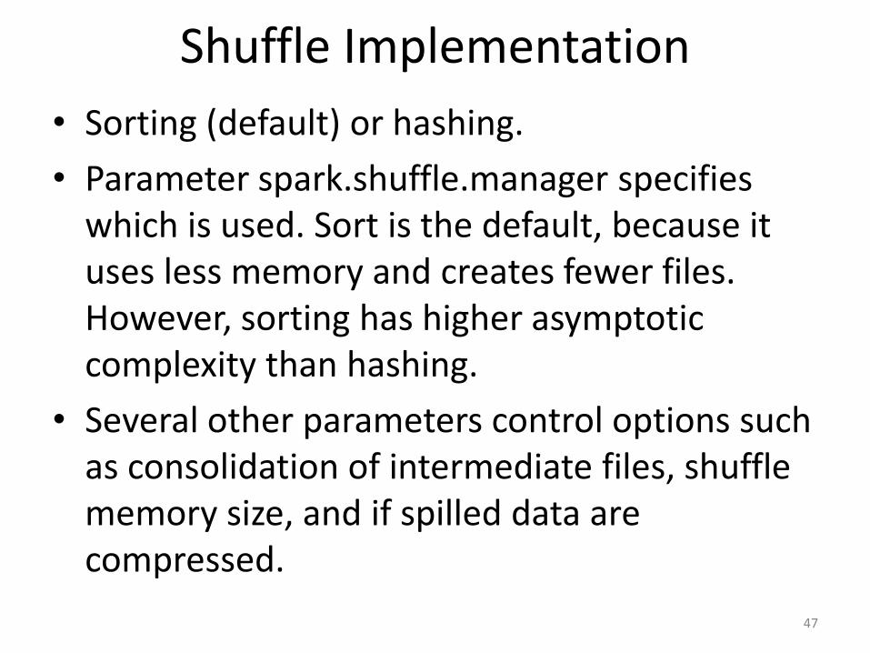
Shuffle Implementation

• Sorting (default) or hashing.

• Parameter spark.shuffle.manager specifies which is used. Sort is the default, because it uses less memory and creates fewer files. However, sorting has higher asymptotic complexity than hashing.

• Several other parameters control options such as consolidation of intermediate files, shuffle memory size, and if spilled data are compressed.

47

48

Next, we explore an important but somewhat more subtle issue: how does Spark pass data and functions to tasks (executors)?

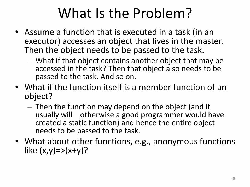
What Is the Problem?• Assume a function that is executed in a task (in an

executor) accesses an object that lives in the master. Then the object needs to be passed to the task.– What if that object contains another object that may be

accessed in the task? Then that object also needs to be passed to the task. And so on.

• What if the function itself is a member function of an object?– Then the function may depend on the object (and it

usually will—otherwise a good programmer would have created a static function) and hence the entire object needs to be passed to the task.

• What about other functions, e.g., anonymous functions like (x,y)=>(x+y)?

49

Let’s Make This Concrete

• We explore the behavior of Spark with some example programs. These are from or inspired by the Spark Programming Guide.

• For the following, pay attention to where the data lives and how it is communicated between application master (driver) and tasks (executors).

50

Object References

51

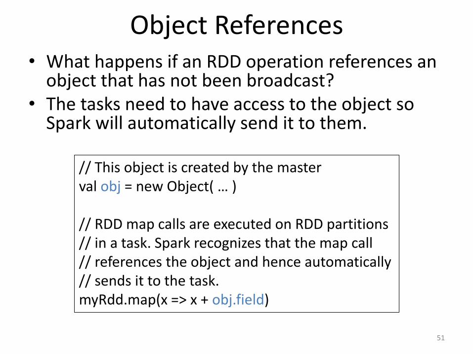
• What happens if an RDD operation references an object that has not been broadcast?

• The tasks need to have access to the object so Spark will automatically send it to them.

// This object is created by the masterval obj = new Object( … )

// RDD map calls are executed on RDD partitions// in a task. Spark recognizes that the map call// references the object and hence automatically// sends it to the task.myRdd.map(x => x + obj.field)

Big Object Reference

52

• If the object is big, this will create a lot of data traffic. What if we only need a small part of the object?

WordCount

Add a value to the counts

Data Movement

53

Master

Task 1

obj

useful

countsRDD_1obj

useful

Task 2

countsRDD_2obj

useful

mapValues() mapValues()

The Program in Action

• Local run with 5 threads, 5 tasks:

54

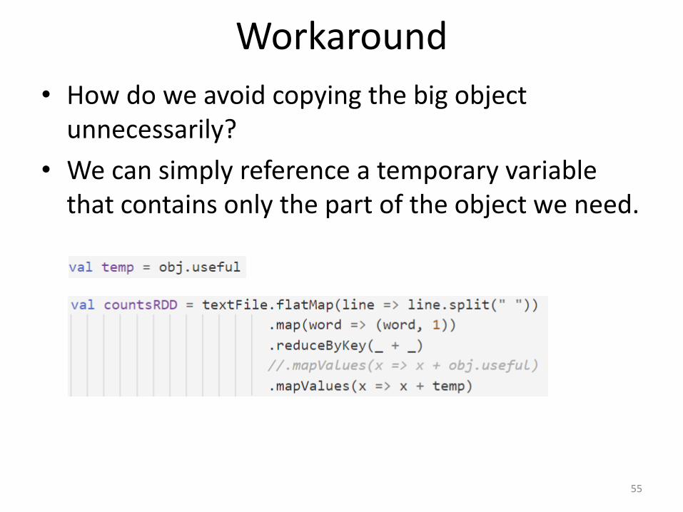
Workaround

• How do we avoid copying the big object unnecessarily?

• We can simply reference a temporary variable that contains only the part of the object we need.

55

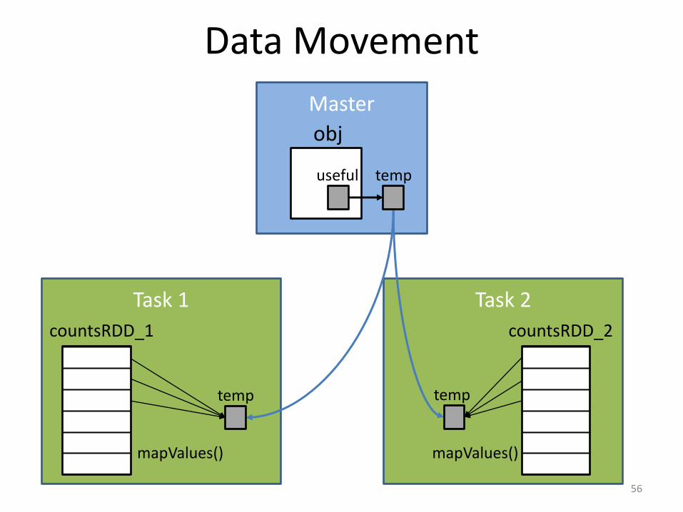
Data Movement

56

Master

Task 1

obj

useful

countsRDD_1

Task 2

countsRDD_2

mapValues() mapValues()

temp

temp temp

The Workaround in Action

• Local run with 5 threads, 5 tasks:

57

~10 times faster

Referencing an Object Method• The same problem occurs when we reference a

method of an object, even if it does not access the object’s internal data.– To guarantee correct execution, the entire object must

be passed to the task.

58

Adds up 2 numbers

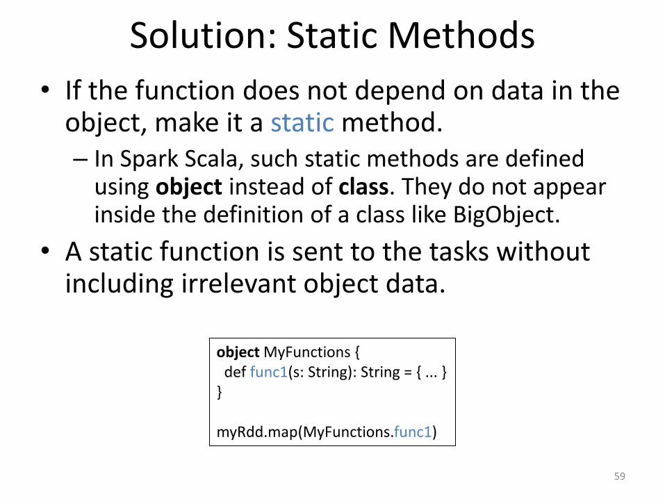
Solution: Static Methods

• If the function does not depend on data in the object, make it a static method.– In Spark Scala, such static methods are defined

using object instead of class. They do not appear inside the definition of a class like BigObject.

• A static function is sent to the tasks without including irrelevant object data.

59

object MyFunctions {def func1(s: String): String = { ... }

}

myRdd.map(MyFunctions.func1)

Anonymous Functions

• Recall examples such asmyRDD.reduce((x,y) => x+y) andmyRDD.map(line => line.split(“ “)). Here “=>” defines an anonymous function.

• Anonymous functions are automatically serialized and passed to each task that applies it to the corresponding partition of the RDD.

– They behave like simple static functions.

60

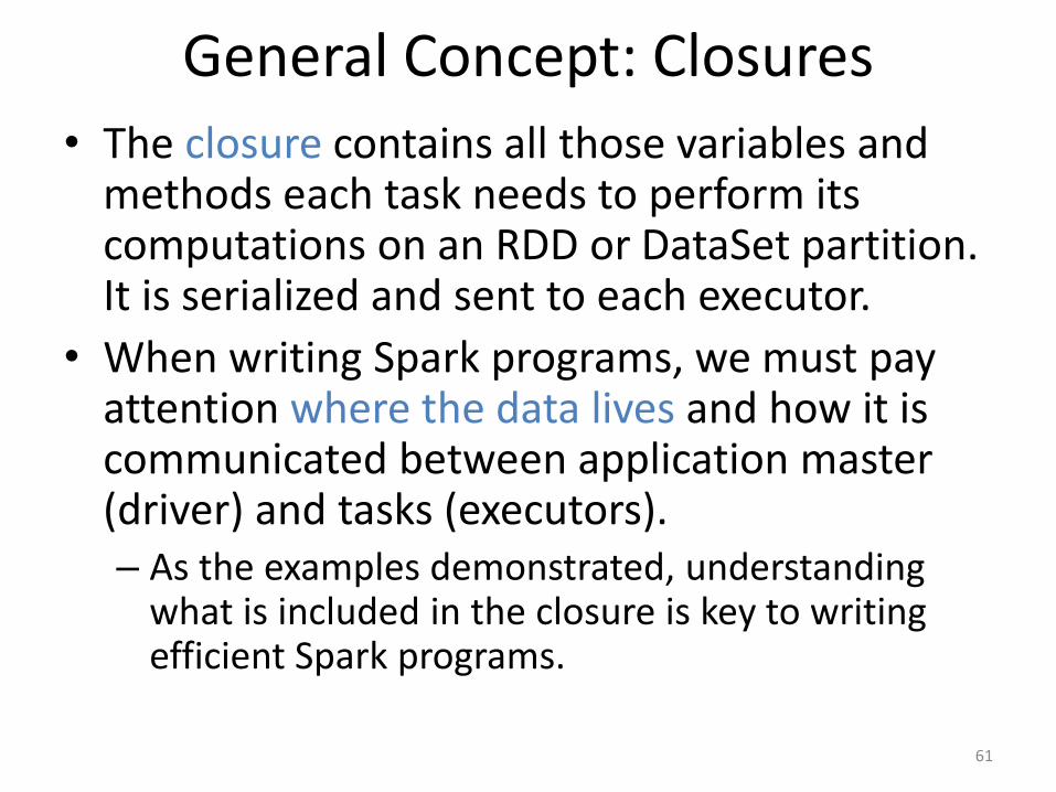
General Concept: Closures

• The closure contains all those variables and methods each task needs to perform its computations on an RDD or DataSet partition. It is serialized and sent to each executor.

• When writing Spark programs, we must pay attention where the data lives and how it is communicated between application master (driver) and tasks (executors).– As the examples demonstrated, understanding

what is included in the closure is key to writing efficient Spark programs.

61

Closure vs Global Variables

• The closure is not the same as a general global variable. It creates a “1-way street” to share data from master to tasks, but it does not provide a “back channel” to let tasks communicate updates to the master or to other tasks.

– It behaves like broadcast variables.

• Let us look at an example to understand this better.

62

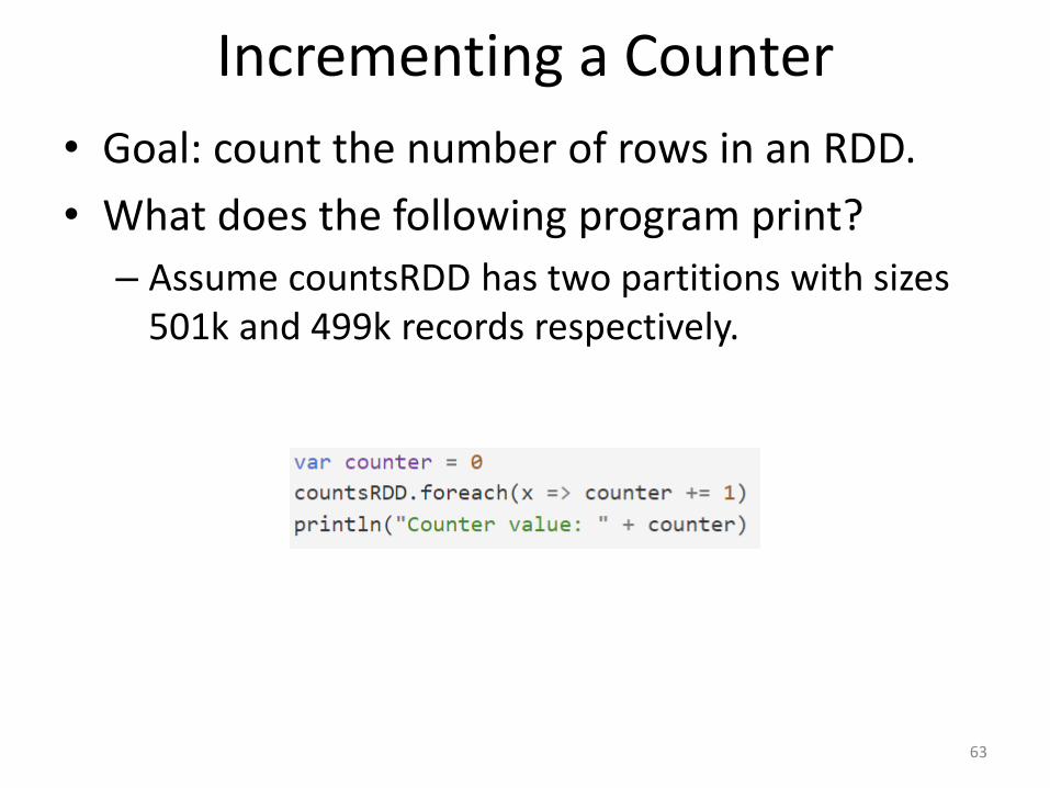
Incrementing a Counter

• Goal: count the number of rows in an RDD.

• What does the following program print?

– Assume countsRDD has two partitions with sizes 501k and 499k records respectively.

63

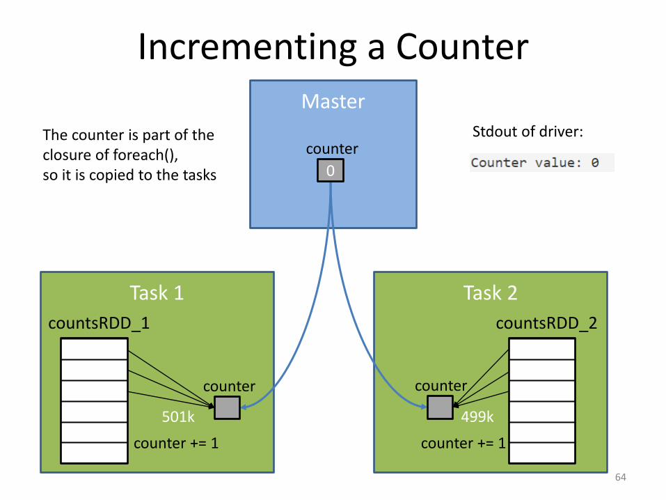
Incrementing a Counter

64

Master

Task 1

countsRDD_1

Task 2

countsRDD_2

counter += 1

0

counter

counter counter

counter += 1

Stdout of driver:The counter is part of the closure of foreach(),so it is copied to the tasks

501k 499k

Workaround

• Closures provide local copies to a task and hence cannot be used to update global state.

• To globally process updates from the tasks, use an Accumulator instead. It is designed to automatically pass its local updates back to the shared global copy in the master.

• Let us look at one more example.

65

Where Is The RDD Printed?

• The first foreach is called in the tasks (executors). Hence the println writes to the executor’s stdout and the RDD content will not show up in the master’s stdout.

• The second foreach collects the RDD on the master, then prints it there.

66

Where Is The RDD Printed?

• The first foreach is called in the tasks (executors). Hence the println writes to the executor’s stdout and the RDD content will not show up in the master’s stdout.

• The second foreach collects the RDD on the master, then prints it there.

67

Lessons Learned

• Make local copies of object members needed by a function, especially when the object islarge and the relevant member is small.

• Use anonymous functions and static methods instead of methods in a class instance.

• Use Accumulators to implement global counters.

• An RDD must be collected if we want one machine to have access to all its data (be careful about memory constraints).

68

69

Next, we explore a bit more the lazy execution of Spark.

PageRank Iterations

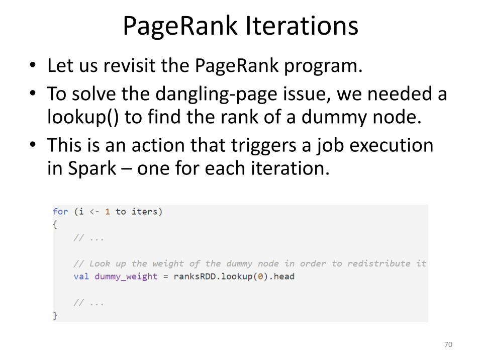
• Let us revisit the PageRank program.

• To solve the dangling-page issue, we needed a lookup() to find the rank of a dummy node.

• This is an action that triggers a job execution in Spark – one for each iteration.

70

PageRank Lineage

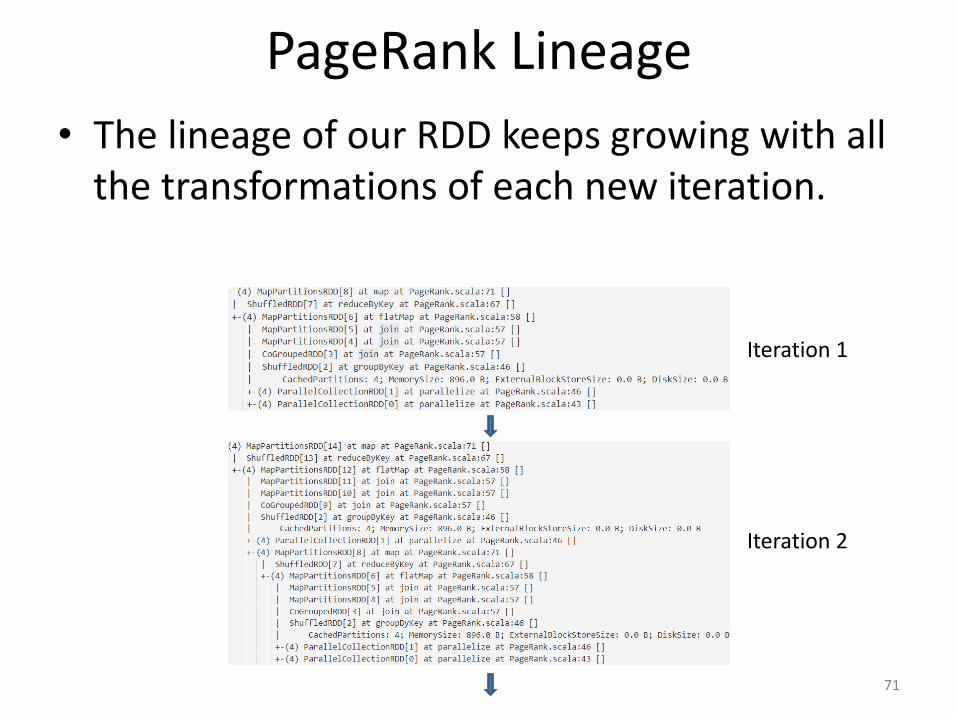
• The lineage of our RDD keeps growing with all the transformations of each new iteration.

71

Iteration 1

Iteration 2

PageRank Lineage Use

• Fault tolerance: if any RDD partition is lost, it can be recomputed using its lineage.

• Optimization: Ideally, the RDD of the previous iteration is stored so that the next iteration does not need to recompute it.

– This in general is not guaranteed and is up to the Spark optimizer.

72

Use of cache()/persist()

• We can give a hint to Spark that certain RDDs should be kept in memory/disk.

• In this case, the log files explicitly tell us if the RDDs are reused.

73

Logs

…

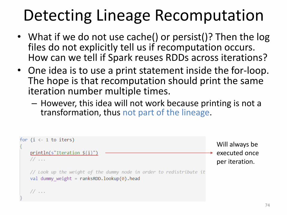
Detecting Lineage Recomputation• What if we do not use cache() or persist()? Then the log

files do not explicitly tell us if recomputation occurs. How can we tell if Spark reuses RDDs across iterations?

• One idea is to use a print statement inside the for-loop. The hope is that recomputation should print the same iteration number multiple times.– However, this idea will not work because printing is not a

transformation, thus not part of the lineage.

74

Will always be executed once per iteration.

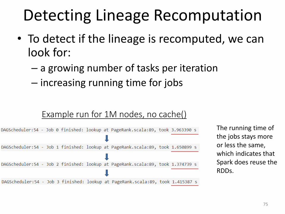
Detecting Lineage Recomputation

• To detect if the lineage is recomputed, we can look for:– a growing number of tasks per iteration

– increasing running time for jobs

75

Example run for 1M nodes, no cache()

The running time of the jobs stays more or less the same, which indicates that Spark does reuse the RDDs.

Detecting Lineage Recomputation• Will Spark always be smart enough to reuse the previous

RDDs? For PageRank most probably yes.• From the Spark Programming Guide:

“Shuffle also generates a large number of intermediate files on disk. As of Spark 1.3, these files are preserved until the corresponding RDDs are no longer used and are garbage collected. This is done so the shuffle files don’t need to be re-created if the lineage is re-computed … automatically persists some intermediate data in shuffle operations (e.g. reduceByKey), even without users calling persist. This is done to avoid recomputing the entire input if a node fails during the shuffle. ”

• Since our PageRank program performs shuffling in each iteration, the RDDs will be stored on disk even if there is not enough memory to cache them.

76

Summary• Spark provides powerful functionality and makes

it easy to write programs for distributed data-intensive computations in the cloud. In addition to core functionality, a variety of libraries have been added, e.g., for SQL, machine learning, graph and stream processing.

• Writing efficient Spark programs and identifying the root cause of poor performance or memory errors requires deeper understanding of Spark’s lineage, lazy evaluation, and closure.– In addition, one must be aware where data lives and

where functions are executed (master vs. tasks/executors).

77

References

• Biswanath Panda and Joshua S. Herbach and Sugato Basu and Roberto J. Bayardo. PLANET: Massively Parallel Learning of Tree Ensembles with MapReduce. Proc. Int. Conf. on Very Large Data Bases (VLDB), 2009

– https://scholar.google.com/scholar?cluster=11753975382054642310&hl=en&as_sdt=0,22

78