monthly technical report - university of texas at...

1 AQRP Monthly Technical Report Template Revised January 2011

Monthly Technical Report (Due to AQRP Project Manager on the 8th day of the month following the last day of the reporting period.)

PROJECT TITLE Development of Speciated

Industrial Flare Emission

Inventories for Air Quality

Modeling in Texas

PROJECT

NUMBER

10-022

PROJECT

PARTICIPANTS (Enter all institutions

with Task Orders for

this Project)

Lamar University DATE

SUBMITTED

06/05/11

REPORTING

PERIOD

From: 05/01/11.

To: 05/31/11. REPORT

NUMBER

3

Invoice Number that accompanies this Report: CM5086-3

Amount of funds spent during this reporting period: $5,203.74

Detailed Accomplishments by Task (Include all Task actions conducted during the reporting

month.)

1. Collection of Flare Operation/Design/Performance Data (Task 2, waiting for

Comprehensive flare study final report for flare performance data)

Details given in Appendix A

2. Hardware/Software/Data storage (Task 3)

Details given in Appendix B

3. Combustion Mechanism Generation/Validation (Task 4A & 4B)

Details given in Appendix B

4. Geometry Creation & Boundary Conditions (Task 5A)

Details are given in Appendix C

5. Base Case Modeling (Task 6A)

Details are given in Appendix A

Preliminary Analysis (Include graphs and tables as necessary.)

NA

Data Collected (Include raw and refine data.)

1. Collection of Flare Operation/Design/Performance Data (Task 2, see Appendix A for

details)

Identify Problems or Issues Encountered and Proposed Solutions or Adjustments

See Section of the Progress of the Task Order to Date.


Goals and Anticipated Issues for the Succeeding Reporting Period

Goals for the next reporting period:

1. Combustion Mechanism Generation & Validation (Task 4A & 4B)

2. CFD Modeling (Cases prescribed in the Model Development Protocol, Task 6A)

3. Model calibration with comprehensive flare study and literature (wind tunnel) data (Task

5D)

Detailed Analysis of the Progress of the Task Order to Date (Discuss the Task Order

schedule, progress being made toward goals of the Work Plan, explanation for any delays in

completing tasks and/or project goals. Provide justification for any milestones completed more

than one (1) month later than projected.)

1. Receipt of the flare test data (input & performance) was delayed for roughly 1 month.

2. Task 6A & 6C will be affected by this delay.

3. Geometry creation was impacted by lack of flare tip details and CFD mesh limitations.

4. Task 6A & 6C will be affected by this issue.

5. All other tasks are on schedule.

Submitted to AQRP by:

Principal Investigator: Daniel H. Chen.

(Printed or Typed)

Appendix A: May Monthly Report for Task 2


CFD Cases

Both the air and steam based cases are broadly divided in 3 sets, based on the 3 different

Lower Heating values (2100, 600 & 350 BTU/SCF) of the fuel used. Each set further has five

cases, with different vent gas velocity, crosswind and other conditions. These CFD cases are

based on the data provided by AQRP to Lamar University and the details were given in the April

monthly report.

CFD Fluent Simulations: Air based flares

Using the geometry provided in Appendix C, CFD Simulations using FLUENT were started.

Due to unusual high flow rate of air (as air-assist), Case A2.1 was taken as the first/base case.

The conditions for the case A2.1 as provided by AQRP in file “Appendix E Tables E-1,

Comprehensive Flare Study QAPP” were used [1].

Table A.I: Conditions used for Case A2.1

Vent gas velocity 0.1656 m/s

Air-assist Velocity 12.99 m/s

Cross wind Velocity 5.74 m/s

Table A. II: Composition of vent gas- Case A2.1

Vent Gas Composition

Species Mass

Fraction

Propylene 1.00

TNG 0.00

Nitrogen 0.00

CFD Model Parameters

In the CFD simulation package, various types of turbulence and chemistry-turbulence interaction

models are available in CFD packages like FLUENT [2-5]. For the flare simulations the

following models were chosen:

Turbulence: k-Epsilon realizable model

The standard k-Epsilon model is a semi-empirical model based on model transport equations for

the turbulence kinetic energy k and its dissipation rate, Epsilon. The model transport equation

for is derived from the exact equation, while the model transport equation for was obtained

using physical reasoning and bears little resemblance to its mathematically exact counterpart.

In the derivation of the - model, the assumption is that the flow is fully turbulent, and the

effects of molecular viscosity are negligible. The standard - model is therefore valid only

for fully turbulent flows

The term "realizable'' means that the model satisfies certain mathematical constraints on the

Reynolds stresses, consistent with the physics of turbulent flows. Neither the standard -

model nor the RNG - model is realizable.


This model has been extensively validated for a wide range of flows, including rotating

homogeneous shear flows, free flows including jets and mixing layers, channel and boundary

layer flows, and separated flows. For all these cases, the performance of the model has been

found to be substantially better than that of the standard - model. Especially noteworthy is

the fact that the realizable - model resolves the round-jet anomaly; i.e., it predicts the

spreading rate for axis symmetric jets as well as that for plan jets.

Turbulence-chemistry interaction: Eddy Dissipation Concept Model

The eddy-dissipation-concept (EDC) model is an extension of the eddy-dissipation model to

include detailed chemical mechanisms in turbulent flows. It assumes that reaction occurs in small

turbulent structures, called the fine scales. The length fraction of the fine scales is modeled as

where denotes fine-scale quantities and

= volume fraction constant = 2.1377

= kinematic viscosity

The volume fraction of the fine scales is calculated as . Species are assumed to react in the

fine structures over a time scale

where is a time scale constant equal to 0.4082.

In EDC model, combustion at the fine scales is assumed to occur as a constant pressure reactor,

with initial conditions taken as the current species and temperature in the cell. Reactions proceed

over the time scale , governed by the Arrhenius rates of Equation, and are integrated

numerically using the ISAT algorithm. ISAT can accelerate the chemistry calculations by two to

three orders of magnitude, offering substantial reductions in run-times. The source term in the

conservation equation for the mean species , Equation is modeled as


where is the fine-scale species mass fraction after reacting over the time .

CFD Solver

During the simulations, the Green-Gauss Cell based solver was used. Apart from that, the

discretization method for Pressure equations was changed from standard to PRESTO!, which is

considered as more robust than the standard model.

Under Relaxation Factors

The under relaxation factors are used to stabilize the convergence behavior of the various

discretized equations like Pressure, Density, Turbulence kinetic energy, Energy etc. Since, the

URFs play an important role; these were changed from time to time, depending on the

convergence stage of the problem.

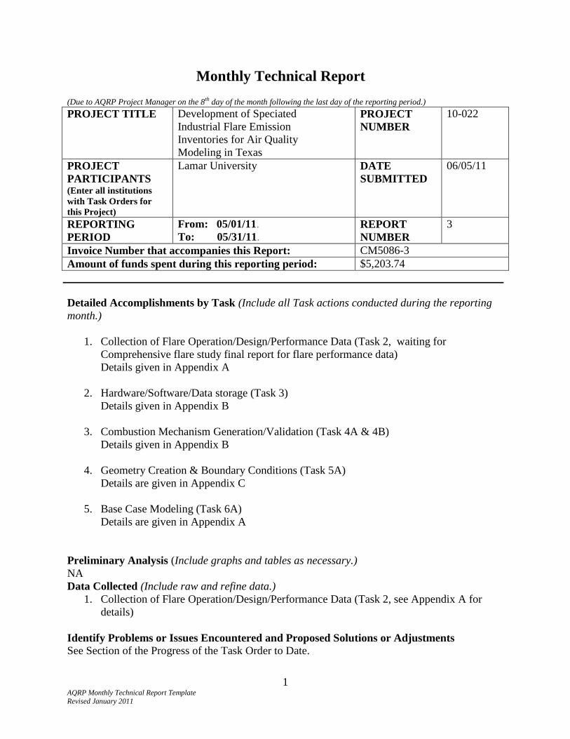
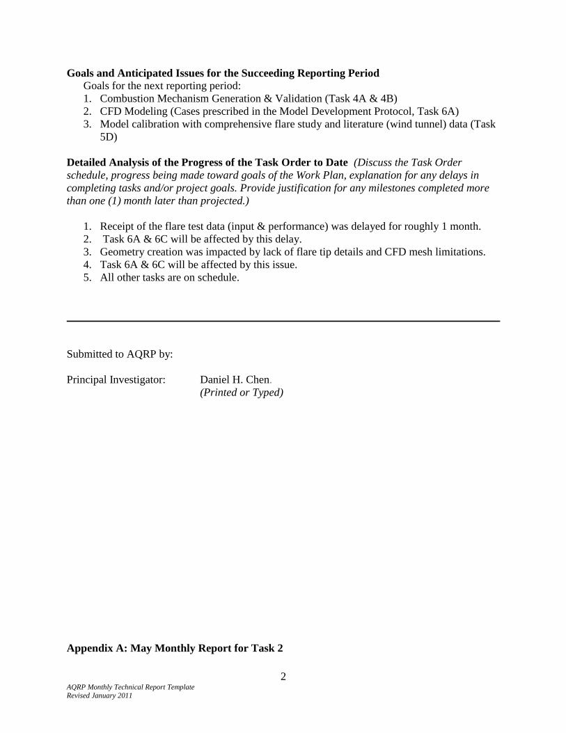
Case A2.1 Results

The preliminary results of the first case including estimated emissions, flare efficiencies, and

temperature/CO2 mass fraction contours are given as follows:

Emissions

Fuel(C3H6) in 360.17 lb/hr

C3H6 out 3.05 lb/hr

CO2 out 1055.12 lb/hr

C in (as C3H6) 308.72 lb/hr

C out (as CO2) 287.76 lb/hr

The two efficiencies were calculated as:

CFD

Simulations TULSA Tests

DRE 99.15% 97.15%

CE 93.21% 95.54%

Destruction and

Removal

Efficiency

=

C3H6 fed - C3H6 out

C3H6 fed

Combustion

Efficiency =

Carbon out as CO2

Carbon fed as fuel


Figure A.1: Contours of Static Temperature (K)

Figure A.2: Contours of Static Temperature (K) zoomed near the flare


Figure A.3: Contours of Mass fraction of CO2

Figure A.4: Contours of Mass fraction of CO2 (zoomed in near the flame)


References

1) Quality Assurance Project Plan, Texas Commission on Environmental Quality

Comprehensive flare Study Project, PGA No. 582-8-862-45-FY09-04, Tracking No. 2008-81

UT/TCEQ/John Zink).

2) ANSYS FLUENT 6.3 User’s Guide, Chapter 12- Modeling Turbulence, Fluent Inc (2006)

3) T.-H. Shih, W. W. Liou, A. Shabbir, Z. Yang, and J. Zhu, A New - Eddy-Viscosity Model

for High Reynolds Number Turbulent Flows - Model Development and Validation. Computers

Fluids, 24(3):227-238, 1995

4) ANSYS FLUENT 6.3 User’s Guide, Chapter 14: Modeling Species Transport and Finite Rate

Chemistry, Fluent Inc (2006).

5) B. F. Magnussen. On the Structure of Turbulence and a Generalized Eddy Dissipation

Concept for Chemical Reaction in Turbulent Flow. Nineteenth AIAA Meeting, St. Louis, 1981


Appendix B: May Monthly Report for Tasks 3, 4A, & 4B

Hardware/Software/Data Storage

All the input data received and data generated in this report (e.g., mechanism validation) are

properly stored in Servers/computers at Lamar University. The data will be stored in external

hard drives for three years. As mentioned in the QAPP, the data will include various fluent case

runs and excel files containing data analysis.

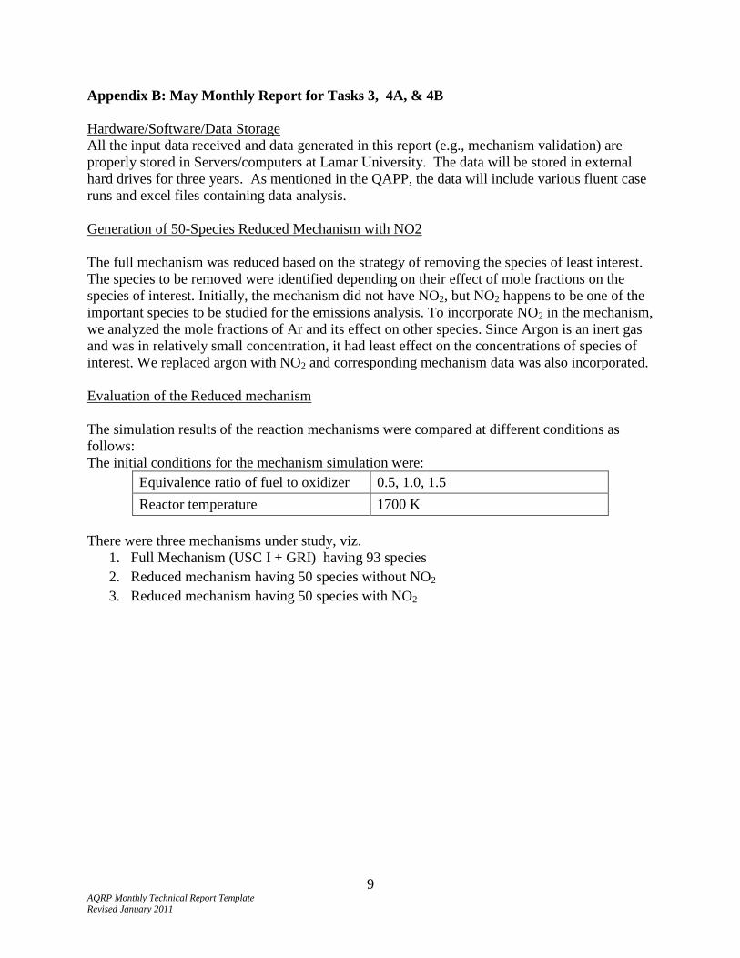
Generation of 50-Species Reduced Mechanism with NO2

The full mechanism was reduced based on the strategy of removing the species of least interest.

The species to be removed were identified depending on their effect of mole fractions on the

species of interest. Initially, the mechanism did not have NO2, but NO2 happens to be one of the

important species to be studied for the emissions analysis. To incorporate NO2 in the mechanism,

we analyzed the mole fractions of Ar and its effect on other species. Since Argon is an inert gas

and was in relatively small concentration, it had least effect on the concentrations of species of

interest. We replaced argon with NO2 and corresponding mechanism data was also incorporated.

Evaluation of the Reduced mechanism

The simulation results of the reaction mechanisms were compared at different conditions as

follows:

The initial conditions for the mechanism simulation were:

Equivalence ratio of fuel to oxidizer 0.5, 1.0, 1.5

Reactor temperature 1700 K

There were three mechanisms under study, viz.

1. Full Mechanism (USC I + GRI) having 93 species

2. Reduced mechanism having 50 species without NO2

3. Reduced mechanism having 50 species with NO2


The species in these mechanisms are as follows:

Mechanism Number

of

Species

Species list

Full

Mechanism

(USC I + GRI)

93 H2,H,O,O2,OH,H2O,HO2,H2O2,C,CH,CH2,CH2*,CH3,CH4,CO,CO2

,HCO,CH2O,CH2OH,CH3O,CH3OH, C2H,C2H2, H2CC,C2H3,C2H4,

C2H5,C2H6,HCCO, CH2CO, HCCOH, C2O, CH2CHO, CH3CHO,

CH3CO, C3H2, C3H3, pC3H4, aC3H4, cC3H4, aC3H5, CH3CCH2,

CH3CHCH, C3H6, C2H3CHO, C3H7, nC3H7, iC3H7, C3H8, C4H,

C4H2, H2C4O, n-C4H3, i-C4H3, C4H4, n-C4H5, i-C4H5, C4H6,

C4H612, C4H7, C4H81, C6H2, C6H3, l-C6H4, c-C6H4, A1,A1-,

C6H5O, C6H5OH, C5H6, C5H5, C5H4O, C5H4OH, C5H5O, N, NH,

NH2, NH3, NNH, NO, NO2, N2O, HNO, CN, HCN, H2CN, HCNN,

HCNO, HOCN, HNCO, NCO, AR, N2

Reduced

mechanism

without NO2

50 H2, H, O, O2, OH, H2O, HO2, CH, CH2, CH2*,CH3, CH4, CO, CO2,

HCO, CH2O, CH2OH, CH3O, C2H2, H2CC, C2H3, C2H4, C2H5,

C2H6, HCCO, CH2CO, CH2CHO, CH3CHO, C3H3, pC3H4, aC3H4,

aC3H5, C3H6, C3H8, C4H2, n-C4H3, i-C4H3, C4H4, N, NH, NH2,

NO, N2O, HNO, CN, HCN, HNCO, NCO, Ar, N2

Reduced

mechanism

with NO2

50 H2, H, O, O2, OH, H2O, HO2, CH, CH2, CH2*,CH3, CH4, CO, CO2,

HCO, CH2O, CH2OH, CH3O, C2H2, H2CC, C2H3, C2H4, C2H5,

C2H6, HCCO, CH2CO, CH2CHO, CH3CHO, C3H3, pC3H4, aC3H4,

aC3H5, C3H6, C3H8, C4H2, n-C4H3, i-C4H3, C4H4, N, NH, NH2,

NO, N2O, HNO, CN, HCN, HNCO, NCO, NO2, N2

This comparison was done at three different equivalence ratio values 0.5, 1.0, 1.5. The results were studied in terms of Actual error and % error. It was found that at equivalence ratio = 1.0 the mole fractions were close enough to be considered as matching. (Except for the main fuel since the fuel was defined as ethylene). Further comparison was carried out at new values of residence times 0.8 and 1.0


The plots of mole fractions of species, at various equivalence ratio values are as follows:

* The simulation was carried out considering C2H4 as fuel

* In further simulations, C3H6 will be considered as fuel and the equivalence ratio 0.8 and 1.0

References

(1) Smith, G. P, Golden, G. M, Frenklach, M, Moriarty, N. W, Eiteneer, B, Goldenberg,M,

Bowman, T, Hanson, R. K, Song, S, Gardiner, W. C, Lissianski,V. V and Qin, Z.

(2000).http://www.me.berkeley.edu/gri_mech/. Accessed 03 October 2010.

(2) Wang, H. and Laskin, A. (1998). A comprehensive kinetic model of ethylene and acetylene

oxidation at high temperatures, Combustion Kinetics Laboratory, Document, Internal report.

0.000E+00

5.000E-05

1.000E-04

1.500E-04

2.000E-04

2.500E-04

3.000E-04

Mole fraction CH2O

Mole fraction C2H4

Reduced with NO2, ER=0.5

Full mechanism, ER=0.5





0.000E+00

5.000E-10

1.000E-09

1.500E-09

2.000E-09

2.500E-09

Mole fraction C3H6

0.000E+00

2.000E-04

4.000E-04

6.000E-04

8.000E-04

1.000E-03

1.200E-03

1.400E-03

1.600E-03

1.800E-03

Mole fraction NO

0.000E+00

2.000E-08

4.000E-08

6.000E-08

8.000E-08

1.000E-07

1.200E-07

1.400E-07

1.600E-07

1.800E-07

Mole fraction NO2

0.000E+00

2.000E-02

4.000E-02

6.000E-02

8.000E-02

1.000E-01

1.200E-01

1.400E-01

Mole fraction CO

Mole fraction CO2


(3) Anuj Bhargava abd Phillip R. Westmoreland, Measured Flame Structure and Kinetics in a

Fuel –Rich Ethylene Flame, COMBUSTION AND FLAME 113: 333-347, 1998

(4) Davis, S. G. and Law, C. K. (1998), "Determination of and Fuel Structure Effects on Laminar

Flame Speeds of C1 to C8 Hydrocarbons", Combustion Science and Technology, 140(1), 427-

449.

(5) R.S.Barlow,A.N.Karpetis, J.H.Frank, J.Y. Chen,”Scalar Profiles and NO formation in

laminar opposed flow partially premixed methane/air flames” Combustion and flame, 2001.

(6) Hai Wang, Xiaoqing You, Ameya V. Joshi, Scott G. Davis, Alexander Laskin, Fokion

Egolfopoulos & Chung K. Law, USC Mech Version II. High-Temperature Combustion

Reaction Model of H2/CO/C1-C4 Compounds. http://ignis.usc.edu/USC_Mech_II.htm, May 2007

http://ame-www.usc.edu/personnel/wang/index.shtml

http://www.exponent.com/leaders/bios/scott_davis.asp?employeeID=555

http://www.exponent.com/leaders/bios/scott_davis.asp?employeeID=555

http://ame-www.usc.edu/personnel/egolfopoulos/index.shtml

http://ame-www.usc.edu/personnel/egolfopoulos/index.shtml

http://www.princeton.edu/~cklaw/


Appendix C: May Monthly Report for Task 5A

Air assisted flare (Geometry & Boundary Conditions, Task 5A)

In order to match the waste gas flow rate the geometry of flare tip has been modified.

However, no change was taken place in computational domain. The finalized geometry contains

the following key features. Domain is made up of 30 m × 30 m enclosed box. The Flare stack is

placed 5 m away from the left of the domain and its height is 10 m. The big domain has been

chosen to consider the entire flame structure.

Fig C.1: Computational Domain

At the left side of domain, the velocity inlet boundary condition is applied, which considers the

effect of cross wind in the computation. At the bottom of the domain, slip wall boundary

condition is applied to simulate a smooth flow. The boundary conditions on all other sides are

given as pressure outlet.

In this simulation the spider shaped burner is considered as given in the comprehensive

flare study document. Rectangular slit is created for waste gas flow to match the exact waste gas

outlet area. Flare tip is divided in three parts:

1. Fuel/waste gas outlet


2. Air outlet

3. Spider wall

Velocity inlet boundary condition is applied at the flare tip for fuel and air flows and the

rest of the portion is defined as spider wall.

Fig C.2: Flare Stack and Flare Tip

[Ref: Quality assurance project plan Drawing number TCEQ LHTS-24]


The structure of flare tip is as shown below:

Fig C.3: Computational Domain of the Flare Tip

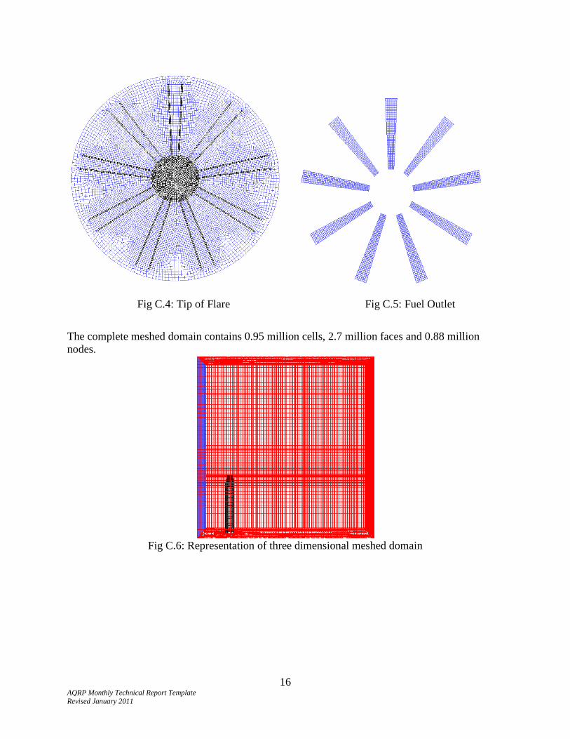
Meshing:

In this study, Gambit 2.3.16 is used for the meshing. Firstly, the base of the domain is

meshed. Different size functions are used to create structure and linked mesh. Then the meshed

base is extended up to the tip of the flare. The entire volume is meshed using cooper algorithm.

The tip of flare meshed using very refined mesh. Meshing is done in such a way that the aspect

ratio will be equal to one at tip of flare. Total nine spiders are created for fuel outlet. The meshed

tip of flare is shown as below:

Fuel

Outlet

Spider Wall

Air Outlet


The complete meshed domain contains 0.95 million cells, 2.7 million faces and 0.88 million

nodes.

Fig C.6: Representation of three dimensional meshed domain

Fig C.4: Tip of Flare Fig C.5: Fuel Outlet

monthly technical report - university of texas at...

Documents