monte carlo generators and soft qcd - lu

Monte Carlo Generatorsand Soft QCD

1. Introduction and Parton Showers

Torbjorn Sjostrand

Department of Astronomy and Theoretical PhysicsLund University

Solvegatan 14A, SE-223 62 Lund, Sweden

CERN, 2 September 2013

Course Plan

Improve understanding of physics at the LHC

Complementary to the “textbook” picture of particle physics,since event generators are close to how things work “in real life”.Notably “soft QCD”, only realistically addressed by generators.

Lecture 1 Introduction and generator surveyParton showers: final and initial

Lecture 2 Combining matrix elements and parton showersLecture 3 Multiparton interactions and other soft physics

HadronizationConclusions

Some prior contact with generators assumed. To learn more:

A. Buckley et al., “General-purpose event generators for LHC physics”,Phys. Rep. 504 (2011) 145 [arXiv:1101.2599[hep-ph]]

or come to a MCnet summer school (see below).

Torbjorn Sjostrand Monte Carlo Generators and Soft QCD 1 slide 2/40

A tour to Monte Carlo

. . . because Einstein was wrong: God does throw dice!Quantum mechanics: amplitudes =⇒ probabilitiesAnything that possibly can happen, will! (but more or less often)

Event generators: trace evolution of event structure.Random numbers ≈ quantum mechanical choices.


The Structure of an Event

An event consists of many different physics steps,which have to be modelled by event generators:


The Monte Carlo method

Want to generate events in as much detail as Mother Nature=⇒ get average and fluctutations right

=⇒ make random choices, ∼ as in nature

σfinal state = σhard process Ptot,hard process→final state

(appropriately summed & integrated over non-distinguished final states)

where Ptot = Pres PISR PFSR PMPIPremnants Phadronization Pdecays

with Pi =∏

j Pij =∏

j

∏k Pijk = . . . in its turn

=⇒ divide and conquer

an event with n particles involves O(10n) random choices,(flavour, mass, momentum, spin, production vertex, lifetime, . . . )LHC: ∼ 100 charged and ∼ 200 neutral (+ intermediate stages)

=⇒ several thousand choices(of O(100) different kinds)


The workhorses: what are the differences?

HERWIG, PYTHIA and SHERPA offer convenient frameworksfor LHC physics studies, but with slightly different emphasis:

PYTHIA (successor to JETSET, begun in 1978):• originated in hadronization studies: the Lund string• leading in development of MPI for MB/UE• pragmatic attitude to showers & matching

HERWIG (successor to EARWIG, begun in 1984):• originated in coherent-shower studies (angular ordering)• cluster hadronization & underlying event pragmatic add-on• large process library with spin correlations in decays

SHERPA (APACIC++/AMEGIC++, begun in 2000):• own matrix-element calculator/generator• extensive machinery for CKKW ME/PS matching• hadronization & min-bias physics under development

PYTHIA and HERWIG originally in Fortran, but now all in C++.


MCnet

MCnet projects:

• PYTHIA (+ VINCIA)

• HERWIG

• SHERPA

• MadGraph

• Ariadne (+ DIPSY)

• Cedar (Rivet/Professor)

Activities include

• summer schools(2014: Manchester?)

• short-term studentships

• graduate students

• postdocs

• meetings (open/closed)

training studentships

3-6 month fully funded studentships for current PhD students at one of the MCnet nodes. An excellent opportunity to really understand and improve the Monte Carlos you use!

www.montecarlonet.orgfor details go to:

Monte Carlo

London

CERNKarlsru

he

LundDurham

Application rounds every 3 months.

MARIE CURIE ACTIONS

funded by:

Manchester Louva

in

Göttingen


Other Relevant Software

Some examples (with apologies for many omissions):Other event/shower generators: PhoJet, Ariadne, Dipsy, Cascade, Vincia

Matrix-element generators: MadGraph/MadEvent, CompHep, CalcHep,Helac, Whizard, Sherpa, GoSam, aMC@NLO

Matrix element libraries: AlpGen, POWHEG BOX, MCFM, NLOjet++,VBFNLO, BlackHat, Rocket

Special BSM scenarios: Prospino, Charybdis, TrueNoir

Mass spectra and decays: SOFTSUSY, SPHENO, HDecay, SDecay

Feynman rule generators: FeynRules

PDF libraries: LHAPDF

Resummed (p⊥) spectra: ResBos

Approximate loops: LoopSim

Jet finders: anti-k⊥ and FastJet

Analysis packages: Rivet, Professor, MCPLOTS

Detector simulation: GEANT, Delphes

Constraints (from cosmology etc): DarkSUSY, MicrOmegas

Standards: PDF identity codes, LHA, LHEF, SLHA, Binoth LHA, HepMC

Can be meaningfully combined and used for LHC physics!


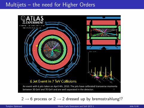
Multijets – the need for Higher Orders

2 → 6 process or 2 → 2 dressed up by bremsstrahlung!?


In the beginning: Electrodynamics

An electrical charge, say an electron,is surrounded by a field:

For a rapidly moving chargethis field can be expressed in terms ofan equivalent flux of photons:

dnγ ≈2αem

π

dθ

θ

dω

ω

Equivalent Photon Approximation,or method of virtual quanta (e.g. Jackson)(Bohr; Fermi; Weiszacker, Williams ∼1934)

e−

e−

e−

e−

.

θ: collinear divergence, saved by me > 0 in full expression.

ω: true divergence, nγ ∝∫

dω/ω = ∞, but Eγ ∝∫

ω dω/ω finite.

These are virtual photons: continuously emitted and reabsorbed.


In the beginning: Bremsstrahlung

(Radio antenna: accelerated charges ⇒ emission of real photons.)When an electron is kicked into a new direction,the field does not have time fully to react:

e−

Initial State Radiation (ISR):part of it continues ∼ in original direction of eFinal State Radiation (FSR):the field needs to be regenerated around outgoing e,and transients are emitted ∼ around outgoing e direction

Emission rate provided by equivalent photon flux in both cases.Approximate cutoffs related to timescale of process:the more violent the hard collision, the more radiation!


In the beginning: Exponentiation

Assume∑

Eγ � Ee such that energy-momentum conservation isnot an issue. Then

dPγ = dnγ ≈2αem

π

dθ

θ

dω

ωis the probability to find a photon at ω and θ,irrespectively of which other photons are present.

Uncorrelated ⇒ Poissonian number distribution:

Pi =〈nγ〉i

i !e−〈nγ〉

with

〈nγ〉 =

∫ θmax

θmin

∫ ωmax

ωmin

dnγ ≈2αem

πln

(θmax

θmin

)ln

(ωmax

ωmin

)Note that

∫dPγ =

∫dnγ > 1 is not a problem:

proper interpretation is that many photons are emitted.

Exponentiation: reinterpretation of dPγ into Poissonian.


QED: Fixed Order Perturbation Theory

Order-by-order perturbative ME calculation containsfully differential distributions of multi-γ emissions,

but integrating the main contributions (leading logs) gives

σ0γ

σ0≈ 1 −αemN +α2

emN2

2 −α3em

N3

6

σ1γ

σ0≈ +αemN −α2

emN2 +α3em

N3

2

σ2γ

σ0≈ +α2

emN2

2 −α3em

N3

2

σ3γ

σ0≈ +α3

emN3

6

which is the expanded form of the Poissonian Pi = 〈nγ〉i e−〈nγ〉 /i !with 〈nγ〉 = αemN.

For practical applications two different regions• large θ, ω ⇒ rapidly convergent perturbation theory• small θ, ω ⇒ exponentiation needed, even if approximate


So how is QCD the same?

A quark is surrounded by a gluon field

dPg = dng ≈8αs

3π

dθ

θ

dω

ω

i.e. only differ by substitution αem → 4αs/3.

An accelerated quark emits gluonswith collinear and soft divergences,and as Initial and Final State Radiation.

e−

q

Typically 〈ng〉 =∫

dng � 1 since αs � αem

⇒ even more pressing need for exponentiation.


So how is QCD different?

QCD is non-Abelian, so a gluonis charged and is surroundedby its own field:emission rate 4αs/3 → 3αs,field structure more complicated,interference effects more important.

αs(Q2) diverges for Q2 → Λ2

QCD,

with ΛQCD ∼ 0.2 GeV = 1 fm−1.

Confinement: gluons below ΛQCD

not resolved ⇒ de facto cutoffs..

Unclear separation between“accelerated charge” and “emitted radiation”:many possible Feynman graphs ≈ histories.

Next: matrix element (ME) and parton shower (PS) descriptions.


Perturbative QCD – 1

Higher orders involve two frontiers• more legs = final-state particles• more loops = virtual corrections

Availability of “exact” calculations for hadron colliders:

Introduction Parton level Parton showers MC@NLO MEPS@LO MEPS@NLO Conclusion

Availability of exact calculations for hadron colliders

donefor some processesfirst solutions

n legs

m loops

1 2 3 4 5 6 7 8 9

1

2

0

F. Krauss IPPP

Matching & Merging of Parton Showers and Matrix Elements

(courtesy Frank Krauss)

Note marked asymmetry between progress along the two axes!


Perturbative QCD – 2

Order-by-order calculations: challenges more math than physics.

LO: solved for all practical applications.

NLO: in process of being automatized.

NNLO: the current calculational frontier.

Another bottleneck: efficient phase space sampling.

gg → H0 illustrates problems:

• Need high-precision calculations

• to search for BSM physics,

• but limited by poorly-understoodslow convergence.


Divergences

Perturbative calculations reliable for hard, well separated jets,but divergent behaviour for θ → 0, ω → 0.

With MEs need to calculate to high order and with many loops⇒ extremely demanding technically (not solved!), and involvingbig cancellations between positive and negative contributions.

Two approaches address these issues:

Resummation: analytical exponentiation;

Parton showers: numerical exponentiation.

i.e. both reinterpret large probabilities as multiple emissions.

Resummation: can be systematically improved order by order,but limited to a few observables;

Parton showers: can address any (parton-level) observable,but typically with less accuracy.


The Parton-Shower Approach

2 → n = (2 → 2) ⊕ ISR ⊕ FSR

FSR = Final-State Radiation = timelike showerQ2

i ∼ m2 > 0 decreasingISR = Initial-State Radiation = spacelike showersQ2

i ∼ −m2 > 0 increasing


Why “time”like and “space”like?

Consider four-momentum conservation in a branching a → b c

p⊥a = 0 ⇒ p⊥c = −p⊥b

p+ = E + pL ⇒ p+a = p+b + p+c

p− = E − pL ⇒ p−a = p−b + p−c

Define p+b = z p+a, p+c = (1− z) p+a

Use p+p− = E 2 − p2L = m2 + p2

⊥

m2a + p2

⊥a

p+a=

m2b + p2

⊥b

z p+a+

m2c + p2

⊥c

(1− z) p+a

⇒ m2a =

m2b + p2

⊥z

+m2

c + p2⊥

1− z=

m2b

z+

m2c

1− z+

p2⊥

z(1− z)

Final-state shower: mb = mc = 0 ⇒ m2a =

p2⊥

z(1−z) > 0 ⇒ timelike

Initial-state shower: ma = mc = 0 ⇒ m2b = − p2

⊥1−z < 0 ⇒ spacelike


Doublecounting

Do not doublecount: 2 → 2 = most virtual = shortest distanceConflict: theory derivations assume virtualities strongly ordered;interesting physics often in regions where this is not true!


The DGLAP equations

Probability of branchings a → bc described by

DGLAP (Dokshitzer–Gribov–Lipatov–Altarelli–Parisi)

dPa→bc =αs

2π

dQ2

Q2Pa→bc(z) dz

Pq→qg =4

3

1 + z2

1− z(neglecting quark masses)

Pg→gg = 3(1− z(1− z))2

z(1− z)

Pg→qq =nf

2(z2 + (1− z)2) (nf = no. of quark flavours)

Universality: any matrix element reduces to DGLAP in collinear limit.

e.g.dσ(H0 → qqg)

dσ(H0 → qq)=

dσ(Z0 → qqg)

dσ(Z0 → qq)in collinear limit


The iterative structure

One-emission expression generalizes to many consecutive emissionsif strongly ordered, Q2

1 � Q22 � Q2

3 . . . (≈ time-ordered).To cover “all” of phase space use DGLAP in whole regionQ2

1 > Q22 > Q2

3 . . ..

Iteration gives(final-state)parton showers:

Iterative structure allows forenergy–momentum conservation,unlike simple exponentiation.

Need soft/collinear cuts to stay away from nonperturbative physics.Details model-dependent, but around 1 GeV scale.


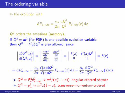
The ordering variable

In the evolution with

dPa→bc =αs

2π

dQ2

Q2Pa→bc(z) dz

Q2 orders the emissions (memory).

If Q2 = m2 (for FSR) is one possible evolution variablethen Q ′2 = f (z)Q2 is also allowed, since∣∣∣∣d(Q ′2, z)

d(Q2, z)

∣∣∣∣ =∣∣∣∣∣ ∂Q′2

∂Q2∂Q′2

∂z∂z

∂Q2∂z∂z

∣∣∣∣∣ =∣∣∣∣ f (z) f ′(z)Q2

0 1

∣∣∣∣ = f (z)

⇒ dPa→bc =αs

2π

f (z)dQ2

f (z)Q2Pa→bc(z) dz =

αs

2π

dQ ′2

Q ′2 Pa→bc(z) dz

Q ′2 = E 2a θ2

a→bc ≈ m2/(z(1− z)); angular-ordered shower

Q ′2 = p2⊥ ≈ m2z(1− z); transverse-momentum-ordered


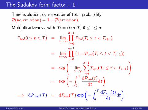
The Sudakov form factor – 1

Time evolution, conservation of total probability:P(no emission) = 1− P(emission).

Multiplicativeness, with Ti = (i/n)T , 0 ≤ i ≤ n:

Pno(0 ≤ t < T ) = limn→∞

n−1∏i=0

Pno(Ti ≤ t < Ti+1)

= limn→∞

n−1∏i=0

(1− Pem(Ti ≤ t < Ti+1))

= exp

(− lim

n→∞

n−1∑i=0

Pem(Ti ≤ t < Ti+1)

)

= exp

(−∫ T

0

dPem(t)

dtdt

)=⇒ dPfirst(T ) = dPem(T ) exp

(−∫ T

0

dPem(t)

dtdt

)Torbjorn Sjostrand Monte Carlo Generators and Soft QCD 1 slide 25/40


Expanded, with Q ∼ 1/t (Heisenberg)

dPa→bc =dQ2

Q2

αs

2πPa→bc(z) dz

× exp

−∑b,c

∫ Q2max

Q2

dQ ′2

Q ′2

∫αs

2πPa→bc(z

′) dz ′

where the exponent is (one definition of) the Sudakov form factor

A given parton can only branch once, i.e. if it did not already do so

Note that∑

b,c

∫ ∫dPa→bc ≡ 1 ⇒ convenient for Monte Carlo

(≡ 1 if extended over whole phase space, else possibly nothinghappens before you reach Q0 ≈ 1 GeV).

Intimately related to e−〈n〉 factor of Poissonian (exponentiation).



Sudakov regulates singularity for first emission . . .

. . . but in limit of repeated softemissions q → qg (but no g → gg)one obtains the same inclusiveQ emission spectrum as for ME,

i.e. divergent ME spectrum⇐⇒ infinite number of PS emissions

Naively exponentiation like in QED,but more complicated in reality:

energy-momentum conservation effects big since αs big,so hard emissions frequent

g → gg branchings leads to accelerated multiplicationof partons

coherence effects important


Coherence

QED: Chudakov effect (mid-fifties)

QCD: colour coherence for soft gluon emission

solved by • requiring emission angles to be decreasingor • requiring transverse momenta to be decreasing


Common Showering Algorithms

Standard shower language with a → bc successive branchings:

HERWIG: Q2 ≈ E 2(1− cos θ) ≈ E 2θ2/2old PYTHIA: Q2 = m2 (+ brute-force coherence)

Newer ARIADNE picture of dipole emission ab → cde:

is the basis for most current-day algorithms (HERWIG excepted)


Parton Distribution Functions

Hadrons are composite, with time-dependent structure:

fi (x ,Q2) = number density of partons iat momentum fraction x and probing scale Q2.

Linguistics (example):

F2(x ,Q2) =∑

i

e2i xfi (x ,Q2)

structure function parton distributions


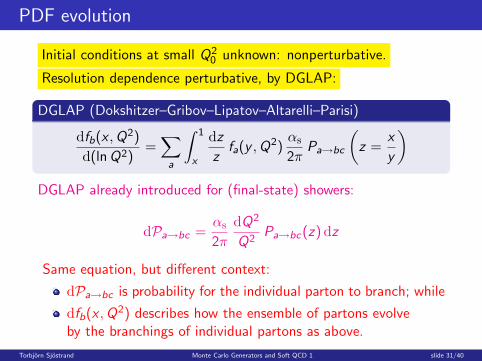
PDF evolution

Initial conditions at small Q20 unknown: nonperturbative.

Resolution dependence perturbative, by DGLAP:

DGLAP (Dokshitzer–Gribov–Lipatov–Altarelli–Parisi)

dfb(x ,Q2)

d(lnQ2)=∑

a

∫ 1

x

dz

zfa(y ,Q2)

αs

2πPa→bc

(z =

x

y

)DGLAP already introduced for (final-state) showers:

dPa→bc =αs

2π

dQ2

Q2Pa→bc(z) dz

Same equation, but different context:

dPa→bc is probability for the individual parton to branch; while

dfb(x ,Q2) describes how the ensemble of partons evolveby the branchings of individual partons as above.


Initial-State Shower Basics

• Parton cascades in p are continuously born and recombined.• Structure at Q is resolved at a time t ∼ 1/Q before collision.• A hard scattering at Q2 probes fluctuations up to that scale.• A hard scattering inhibits full recombination of the cascade.

• Convenient reinterpretation:


Forwards vs. backwards evolution

Event generation could be addressed by forwards evolution:pick a complete partonic set at low Q0 and evolve,consider collisions at different Q2 and pick by σ of those.Inefficient:

1 have to evolve and check for all potential collisions,but 99.9. . . % inert

2 impossible (or at least very complicated) to steer theproduction, e.g. of a narrow resonance (Higgs)

Backwards evolution is viable and ∼equivalent alternative:start at hard interaction and trace what happened “before”


Backwards evolution master formula

Monte Carlo approach, based on conditional probability : recast

dfb(x ,Q2)

dt=∑

a

∫ 1

x

dz

zfa(x

′,Q2)αs

2πPa→bc(z)

with t = ln(Q2/Λ2) and z = x/x ′ to

dPb =dfbfb

= |dt|∑

a

∫dz

x ′fa(x′, t)

xfb(x , t)

αs

2πPa→bc(z)

then solve for decreasing t, i.e. backwards in time,starting at high Q2 and moving towards lower,with Sudakov form factor exp(−

∫dPb)

Webber: can be recast by noting that total change of PDF at x isdifference between gain by branchings from higher x and loss bybranchings to lower x .


Evolution procedures

DGLAP: Dokshitzer–Gribov–Lipatov–Altarelli–Parisievolution towards larger Q2 and (implicitly) towards smaller xBFKL: Balitsky–Fadin–Kuraev–Lipatovevolution towards smaller x (with small, unordered Q2)CCFM: Ciafaloni–Catani–Fiorani–Marchesiniinterpolation of DGLAP and BFKLGLR: Gribov–Levin–Ryskinnonlinear equation in dense-packing (saturation) region,where partons recombine, not only branch


Did we reach BFKL regime?

Study events with ≥ 2 jets as a function of their y separation.

Ratio of the inclusive toexclusive dijet cross sections:

y|Δ|0 1 2 3 4 5 6 7 8 9

incl

R

1

1.5

2

2.5

3

3.5

4

4.5

52010 data

PYTHIA6 Z2

PYTHIA8 4C

HERWIG++ UE-7000-EE-3

HEJ + ARIADNE

CASCADE

= 7 TeVsCMS, pp,

dijets > 35 GeV

Tp

|y| < 4.7

Azimuthal decorrelation:

No strong indications for BFKL/CCFM behaviour onset so far!


Initial- vs. final-state showers

Both controlled by same evolution equations

dPa→bc =αs

2π

dQ2

Q2Pa→bc(z) dz · (Sudakov)

but

Final-state showers:Q2 timelike (∼ m2)

decreasing E ,m2, θboth daughters m2 ≥ 0physics relatively simple⇒ “minor” variations:Q2, shower vs. dipole, . . .

Initial-state showers:Q2 spacelike (≈ −m2)

decreasing E , increasing Q2, θone daughter m2 ≥ 0, one m2 < 0physics more complicated⇒ more formalisms:DGLAP, BFKL, CCFM, GLR, . . .


Combining FSR with ISR

Separate processing of ISR and FSR misses interference(∼ colour dipoles)

ISR+FSR add coherentlyin regions of colour flowand destructively else

in “normal” shower byazimuthal anisotropies

automatic in dipole(by proper boosts)


Coherence tests

Current-day generators for pseudorapidity of third jet:

and pastincoherent:

Coherence tests – 1

old normal showers with/without ' reweighting:⌘3

: pseudorapidity of third jet↵: angle of third jet around second jet

Torbjorn Sjostrand PPP 4: Parton distributions and initial-state showers slide 37/39


Summary and Outlook

A multitude of physics mechanisms at play in pp collisions.

Event generators separate problem into manageable chunks.

Random numbers ≈ quantum mechanical choices.

Often need to combine several software packages.

Matrix element calculations at core of process selection.

Parton shower offers convenient alternative to HO ME’s.

Unitarity by Sudakov form factor.

Next (this afternoon):

Combining matrix elements and parton showers.


monte carlo generators and soft qcd - lu

Documents