Towards Automated Language Classification: A Clustering Approach

Armin Buch, David Erschler, Gerhard Jäger, and Andrei Lupas

1 Introduction

In this paper, we discuss advantages of clustering approaches to automated language classification, describe distance measures used for this purpose, and present results of several proof-of-concept experiments. We advocate the use of probability based distances – those that take into account the dis-tribution of relevant features across the language sample in question.

Phylogenetic tree algorithms have become a popular tool in computer-aided historical linguistics to discover and visualize large-scale patterns among large groups of languages. The technique crucially uses similarity measures, see, for instance, MacMahon & MacMahon 2005, Forster and Renfrew (2006) and Nichols & Warnow (2008).

While being powerful tools, phylogenetic algorithms have a few disad-vantages. This is well-known in bioinformatics, and perhaps even more pressing in linguistic applications. To start with, phylogenetic algorithms are designed to discover tree-like signals. Non-tree shaped structures (due to lateral transfer, parallel or convergent evolution, or chance) are system-atically misinterpreted. Furthermore, phylogenies lose resolution in the deep nodes as the number of sequences increases, because branching deci-sions are always taken hierarchically from the leaves to the root and there-fore the effects of contradicting data accumulate as the computation pro-gresses towards the root. Also, phylogenies become more inaccurate with the number of sequences because the multiple alignments on which they are based accumulate errors, the likelihood of including false positive se-quences, which distort the topology of the tree, increases, and highly diver-gent sequences are shuffled to the root of the tree where they are artificially joined into a basal clade (long branch attraction). Last but not least, in phy-logenetic analyses the time needed to find the optimal tree increases expo-

nentially with the number of sequences1, so that trees of more than a few thousand sequences become computationally prohibitive.

Frickey and Lupas (2004) devised the software package CLANS (CLus-ter ANalysis of Sequences) that visualizes similarities between data points by projecting them onto a low-dimensional (2d or 3d) cluster map. Using a force-directed graph layout algorithm, groups of similar data points form clusters that are easy to identify visually or via standard clustering meth-ods. Cluster maps do not suffer from the above-mentioned problems. In particular, errors do not accumulate but cancel out each other, and the com-putational complexity is not worse than quadratic (Fruchtermann and Rein-gold 1991). CLANS has been applied successfully to the analysis of phylo-genetic relationships between protein sequences and other biological char-acteristics of organisms.

It is obviously possible to feed appropriately encoded linguistic data into clustering software. However, it is not clear a priori to which extent clustering methods are applicable in linguistics and how useful they are for research.

We argue that this kind of technique would indeed be useful and illus-trate it with a number of proof-of-concept experiments. We show that, when based on lexical data, our technique essentially reproduces the classi-cally known relationships between Indo-European languages. On the other hand, applying the procedure to morphosyntactic features does not provide anything remotely approaching a genetic classification, as expected. Fur-thermore, we argue that CLANS allows to better visualize results than SplitsTree (Huson & Bryant 2006) an application that has become very common in the field (Nichols & Warnow 2008).

From the very outset, we should stress the point that findings procured from CLANS clusterings are statistical by their nature. That is to say, the larger a cluster is, and the more connections does the algorithm produce for it, the more significant are the findings. Unfortunately, at least in its present form our method cannot be used in elucidating the genetic relation-ship of language isolates.

In bioinformatics, a very large amount of input data is granted, given the very large number of proteins in living organisms and the length of protein sequences. In linguistics, assembling a database that would be amenable to meaningful statistical processing is a much more challenging task. We used three readily available databases: the database of Gray and

Atkinson2 (2003) on Indo-European languages, which is based on the well-known database of Dyen, Kruskal, and Black (1992), further on to be called the DKB database; the morphosyntactic feature database from WALS (Haspelmath et al. 2008) and the Automated Language Classifica-tion Database of Wichmann et al,3, further on to be called the ASJP data-base.

The paper is organized as follows: In Section 2, we describe main fea-tures of CLANS software and comment on the key technical ingredient: similarity or distance matrices. Then we proceed to examine a number of test cases. In Section 3, we explore binary feature based distances. The datasets in question are the DKB database and a subsample of WALS. Us-ing the latter sample, we compare the results of CLANS with a network produced by SplitsTree. In Section 4, we investigate a measure of language similarity based on distances between words. We show that the findings for Indo-European languages are in a good agreement with the traditional clas-sification. In Section 6, we investigate language distances based on unsu-pervised alignment of parallel texts. Section 7 concludes.

2 Introducing CLANS

2.1 Second-grade heading

CLANS is an implementation of the Fruchterman–Reingold (1991) graph layout algorithm. It has been designed for discovering similarities between protein sequences.

Sequences are represented by vertices in the graph, BLAST/PSIBLAST high scoring segment pairs (HSPs) are shown as edges connecting vertices and provide attractive forces proportional to the negative logarithm of the HSP’s P-value. To keep all sequences from collapsing onto one point, a mild repulsive force is placed between all vertices. After random place-ment in either two-dimensional or three-dimensional space, the vertices are moved iteratively according to the force vectors resulting from all pair-wise interactions until the overall vertex movement becomes negligible. While this approach, coupled with random placement, causes non-deter-ministic behavior, similar sequences or sequence groups reproducibly come to lie close together after a few iterations thus generating similar, al -though non-identical graphs for different runs. (Frickey, Lupas 2004)

It is the reproducibility of the overall picture that makes the outcomes of CLANS clustering reliable.

P-values, the usual input data for CLANS, measure the probability that a similarity between two sequences is due to chance. The more non-trivial a similarity is, i.e. the closer the sequences are, the lower gets the p-value. Therefore, p-values can be thought of as measures of distance. In principle, the program is able to operate with any distance-like measure.

3 Binary feature based distances

3.1 Hamming distance

The most straightforward approach to the measurement of distances be-tween languages is to posit a number of binary parameters for each lan-guage. The state of any language would be ideally described by a binary vector, and the Hamming distance between the vectors can be considered as a distance between the respective languages.

The downside is that in all known realizations of this idea, parameters have to be set manually.

An immediate technical problem is that it is almost always the case that for some languages, the values of some of the parameters are missing: they could be either unknown (due to a gap in a wordlist or a grammatical de-scription), or non-defined altogether. (For instance, it is meaningless to dis-cuss the locus of complementizer placement in a language that does not use complementizers at all.)

One way to circumvent this problem is to normalize the Hamming dis-tance ''', LLH between a pair of languages, 'L and ''L , by the overall number of parameters N . Then the normalized distance will be

We applied this distance to cognation judgments that are built into the DKB database. This is a natural step to take, because it is essentially cog-nation judgments that underlie classifications in traditional historical lin-guistics.

The picture for Indo-European languages we obtained (see Fig. 1) re-produces the classically known one in a reasonably satisfactory manner: All subgroups of Indo-European that are presented in the database by suffi-ciently many varieties (these are Albanian, Germanic, Greek, Indic, Ira-nian, Romance, and Slavic), are realized as separate clusters.

3.2 Feature distribution across the language sample as a source of distances

A frequently explored alternative to cognation judgments is morphosyntac-tic features [see, among others, Dunn et al. (2008), Dunn (2009), Langob-ardi and Guardiano (2009), and Greenhill et al (2011)]. It is thus natural to test our technique against this source of distance.

For 133 languages that contain sufficiently many feature values in WALS, we computed a pairwise similarity matrix. The similarity of two languages is defined as the sum of weights of all WALS features where both languages have defined but different values. The weight w(f) of a fea-ture f is defined as the mutual information between the value of this feature and the language family affiliation (as listed in the WALS database) of the languages in question.

Figure 1. Clustering of the DKB database.

In this way, features which contain much information about the genetic affiliation of languages receive a high weight (and vice versa). This deci-sion was motivated by the hope to extract a deep genetic signal from the WALS data.

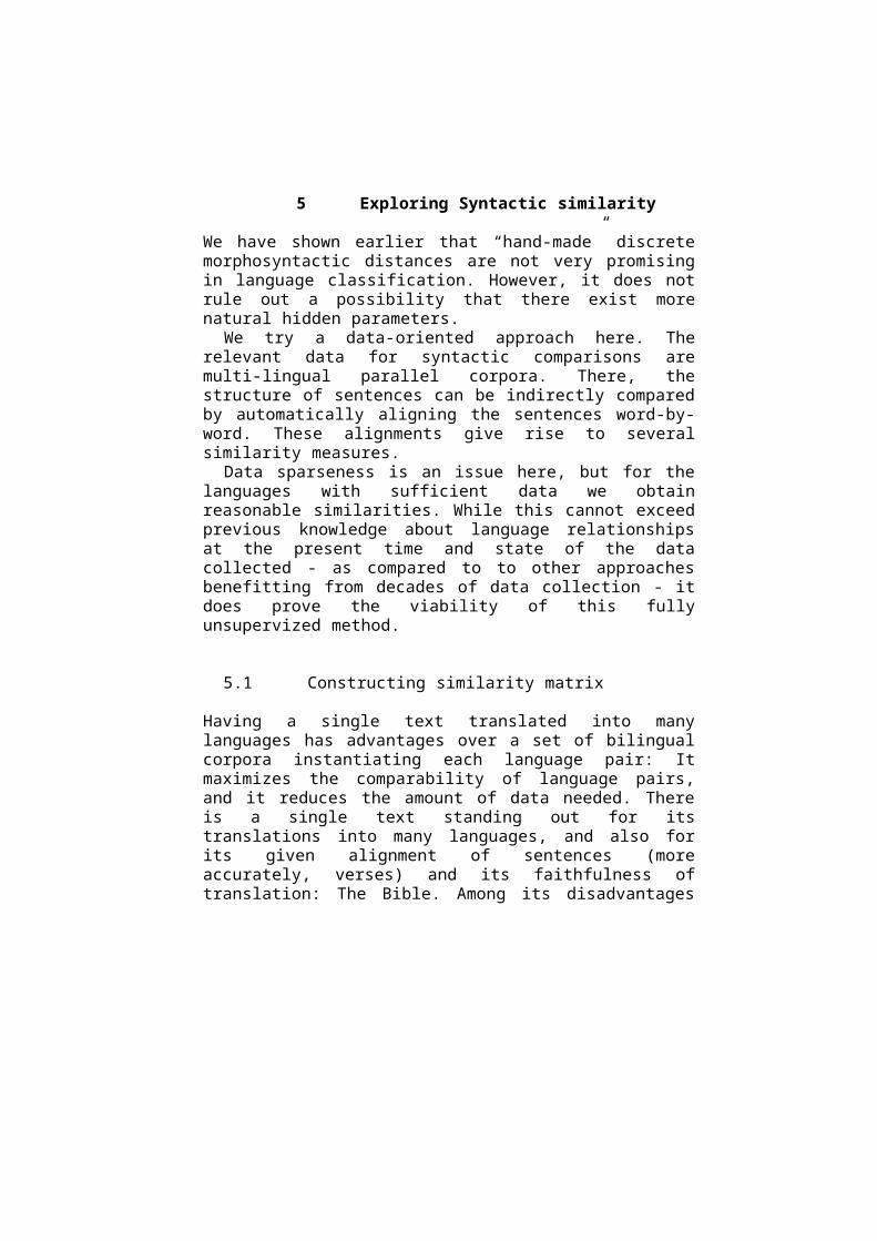
The resulting cluster map (see Fig. 2) shows a circular structure. There are two large clusters of languages at opposite sides of the circle (shown in gray and black), and a third, smaller cluster (shown in white) in between. The other languages are arranged somewhere on the circle between these three regions without forming distinct groups.

The map on Fig 3 shows the geographic distribution of respective lan-guages (colors on the map match the colors on Fig. 2).2

A manual inspection of this outcome reveals that this cluster map cap-tures a strong typological and a somewhat weaker areal signal, but no us-able information about genetic affiliations. The cluster shown in grey con-tains languages with head-initial basic word order (SVO or VSO), small phoneme inventories, and lack of case marking. The black cluster, on the other hand, is characterized by head-final word order, nominative-accusa-

Figure 2. CLANS clustering of WALS.

Figure 3. Geography of the language sample.

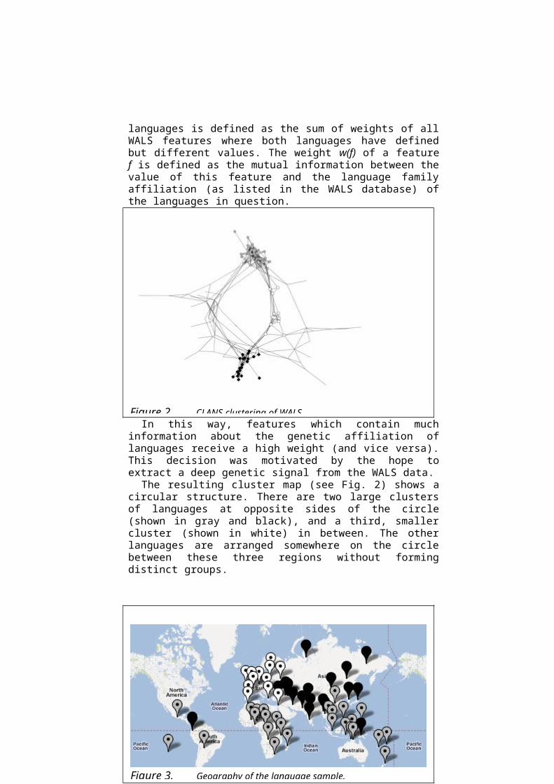
tive alignment both for pronouns and full NPs, a large number of cases (mostly more than 6) and predominant dependent marking. Figure 2 shows that these groupings are neither genetically nor areally motivated.

That perfectly well agrees with the findings of Greenhill et al (2011) and Donohue et al (2011): The distribution of morphosyntactic features does not sufficiently well reflect genetic relationships between languages.

It should be stressed that this conclusion does not mean that mor-phosyntactic features of proto-languages are not amenable for reconstruc-tion ‒ it only means that (a) the possible depth of reconstruction is less than that for words and (b) the inventory of morphosyntactic features is much more restricted than that of possible words, and thus morphosyntac-tic features are more prone to chance coincidences.

Somewhat paradoxically, that also does not mean that morphosyntactic features are less evolutionary stable than lexical one: a morphosyntactic feature may persist in a language population, only its “carriers” change.

This expectation is also compatible with Johanna Nichols’ (1992) con-cept: it is possible to imagine that certain features may persist in certain zones, and get acquired by languages when the latter move into respective zones.

3.3 Comparing CLANS with Splits Tree

In this subsection, we use WALS data to argue for advantages of CLANS clustering. Given that the use of SplitsTree has become a near-standard in the field, it is worth comparing its output with that of CLANS. Besides computational advantages, already mentioned in the introduction, we con-tend that CLANS pictures better visualize findings. To illustrate this point, we present here the network created with SplitsTree for WALS features, see Figure 3. We contend that the SplitsTree network brings out the pat-terns that are inherent in the WALS data, much less clearly.

Figure 4. SplitsTree network for the WALS data

4 Word Similarity Based Measures

For any method of automated classification to be of practical interest to re-searchers, it has to be applicable to large datasets from little studied lan-guages. Consequently, cognation judgments cannot be built in into the databases. Additionally, given the difficulty of assembling any sufficiently large database, it is virtually unavoidable that such methods must work with word lists – this is the only type of data that is relatively easy to col-lect. Therefore, the task of defining a distance between languages gets re-duced to defining a distance between word lists.

It is intuitively clear that, first, any distance between wordlists should be based on pairwise distances between words with the same meaning, and, second, it should somehow take into account the average distance between a random pair of words from the two lists.

In this section, we implement this intuition and apply the resulting simi-larity measure to Indo-European languages from the ASJP database. The latter includes 40 basic meanings from the Swadesh list for each language, see details in Wichmann et al (2010: 3633).

4.1 Constructing similarity matrix

4.1.1 Levenshtein distance

A basic ingredient for this matrix is the Levenshtein distance. Recall that the Levenshtein distance is defined in the following way: for two strings,

1s and 2s (of symbols from a same alphabet A) . The following opera-tions are permitted: replace a letter of 2s by another one, delete a letter of

2s ; add a letter to 2s . The distance 21, ssL is the minimal number of such operations necessary to create 1s from 2s . The Levenshtein dis-tance has been applied to language classification problems in a number of works, see, among others, Petri and Serva (2010) and Wichmann et al. (2010).

For example, if the alphabet consists of letters a and b, then 0, aaL ; 1, baL , because we have to replace a by b in the sec-

ond word, and 2, baabL , we have, for instance, to delete the first b

in ba and then add b to the right of a, and it is impossible to achieve the re-sult by only one operation.

4.1.2 Preparing data

Now, lists of 40 meanings are accumulated for all languages of the sample – if a word list for a particular language contains more items, they are ex-cluded from further consideration. (However, even these shorter 40-word lists sometimes contain gaps.)

Now, all vowels are treated as a single class; all consonants are col-lapsed into four classes: bilabials (b, p, f, v); nasals (m, n); fricative velars and uvulars (x, ʁ, etc), the rest of consonants are collapsed into one more class.

4.1.3 Computation of similarity

For each pair of languages, L’ and L’’, only the meanings present in both lists are kept. Let M denote the number of remaining meanings. For each remaining pair of words iv and jw , the Levenshtein distance ji wvL , is computed – disregarding whether or not the two words cor-

respond to a same meaning. The similarity ji wv , is then defined in the, following manner:

Thus, the similarity is 1 if the words are identical and 0 if they are totally different.

Now consider the similarity value iii wv , for a specific poten-tial cognate pair iv , iw . (Now these are two words with a same mean-ing!) By itself, this value is not very telling. What we want to estimate, is how likely it is for a random pair of words from the two languages to have the same (or higher) similarity value. We estimate this probability, ip , as the number of pairs with the similarity greater or equal to i , divided by the overall number of pairs.

The lower the value of pi is, the higher is the chance that the similarity be-tween vi and wi is non accidental. Assuming that similarities among differ-ent pairs of potential cognates are independent, we take the product of pi’s for all meanings out of the 40 for which we have data. Let P denote this product.

Now, we define the similarity SL’L’’ between L’ and L’’ as -log(P) (the minus sign serves to make the thing positive). The values SL’L’’ serve as the input for CLANs.

The method we use might look suspiciously similar to Greenberg’s (1987) ‘mass comparison”, justly criticized by many authors, for a detailed discussion and reference see, for example, Campbell and Poser (2008). The crucial difference between our approach and Greenberg’s mass comparison is that, unlike in Greenberg’s work, the similarity between words is estab-

Figure 5. Indo-European language cluster with respect to the Word Similarity measure.

lished by an algorithm and not a human. That makes results considerably more reproducible (as long as the same initial dataset is used.)

5 Exploring Syntactic similarity

We have shown earlier that “hand-made” discrete morphosyntactic dis-tances are not very promising in language classification. However, it does not rule out a possibility that there exist more natural hidden parameters.

We try a data-oriented approach here. The relevant data for syntactic comparisons are multi-lingual parallel corpora. There, the structure of sen-tences can be indirectly compared by automatically aligning the sentences word-by-word. These alignments give rise to several similarity measures.

Data sparseness is an issue here, but for the languages with sufficient data we obtain reasonable similarities. While this cannot exceed previous knowledge about language relationships at the present time and state of the data collected - as compared to to other approaches benefitting from decades of data collection - it does prove the viability of this fully unsuper-vized method.

5.1 Constructing similarity matrix

Having a single text translated into many languages has advantages over a set of bilingual corpora instantiating each language pair: It maximizes the comparability of language pairs, and it reduces the amount of data needed. There is a single text standing out for its translations into many languages, and also for its given alignment of sentences (more accurately, verses) and its faithfulness of translation: The Bible. Among its disadvantages are un-natural word orderings due to an overly close replication of - say - the Latin Vulgate's syntax, and archaic language.

Syntactically annotated parallel corpora would be preferable in this en-deavor. However, there is little hope of finding such for a reasonable selec-tion of languages. Automatically parsing the corpus is not an option either, because for many languages there are no parsers available. We therefore devise a method to obtain a similarity measure in an unsupervised manner.

The Bible has been considered as a source of parallel texts before. The University of Maryland Parallel Corpus Project (Resnik et al 1999). created a corpus of 13 Bible translations. Their project ended prematurely; only 3 versions agree in verse counts, and many contain artifacts of the automatic processing (parse errors etc.). We enlarged the corpus by translations from several online resources4.

Most corpora required at least some (if not considerable) manual correc-tions. We removed comments and anything else that did not belong to the main text. In the original digitization, there were unrecognized verse/line breaks as well as falsely recognized ones (e.g. at numbers) and numerous other mistakes, which we corrected where possible, but we are fully aware that many errors remain.

Our final corpus format consists of one line per verse, indexed by a shorthand for the book, the chapter, and the verse:

GEN.1.1 In the beginning God created the heaven and the earth.

We chose this format for ease of processing. The encoding is utf-8.Currently our corpus comprises 46 complete (Old and New Testament)

Bible translations in 37 languages, where 'complete' indicates that they contain the same number of verses (31102), yet a few lines still might be empty. Diverging verse numberings in the raw versions obtained from the web resources might also be due to more severe annotation errors. We have checked divergences manually (within the limits of spotting the mistakes in the first place, and being able to correct them due to language accessibil-ity), and hope that the remaining errors will be insignificant in comparison to the overall corpus size.

The languages are: Albanian, Arabic (Afroasiatic, Semitic), Bulgarian, Cebuano (Austronesian, Philipines), Chinese, Czech, Danish, Dutch, Eng-lish, Esperanto, French, German, Haitian Creole, Hindi, Hmar (Tibeto-Bur-man, India), Hungarian (Uralic), Indonesian (Austronesian), Italian, Kan-nada (Dravidian, India), Korean, Lithuanian, Malagasy (Austronesian, Madagascar), Maori (Austronesian, New Zealand), Hebrew (Afroasiatic, Semitic), Norwegian, Persian, Portuguese, Romanian, Russian, Somali (Afroasiatic, Kushitic), Spanish, Tagalog (Austronesian, Philipines), Tamil (Dravidian, India and Sri-Lanka), Telugu (Dravidian, India), Thai (Tai-Kadai), Ukrainian, and Xhosa (Bantu, South Africa).

Some languages are represented several times in the corpus: English with 7 translations; German and Spanish with 2 each. They exemplarily al-low for the study of intra-language variation. See 5.4.2 for a discussion.

5.2 Constructing similarity matrix

We now devise a method to evaluate the similarity of languages based on unannotated parallel corpora, with the assumption that they are already aligned on the sentence level. This method will exhibit the following prop-erties:

- Applicability to any language. This excludes the use of parsers, and even of taggers, because they need to be trained on annotated data. It also rules out the application of language-specific linguistic knowledge.

- Full automatization. As similarities need to be computed for any pair of languages, any manual step would have to be repeated prohibitively of-ten.

- Evaluation of syntactic properties. In spite of the lack of annotation, the method shall reflect similarity on a structural level.

Especially the last point appears to be paradoxical. It seems to presup-pose a step of grammar induction. Yet it is not necessary to know the grammar of a language or to have a parse for every sentence in the corpus in order to know how similar two languages are. Since only surface infor-mation is given, this measure will have to rely on just that. The comparable unit of parallel corpora is the sentence, resp. here, the verse. The similarity of two languages is then defined as an aggregate, e.g. the average, over (all available corpora for these languages and) all sentences.

If a source sentence and a target sentence are translations of each other, they will contain words being translations of each other. Now a word-by-word translation usually is ungrammatical. It differs from an actual transla-tion in the order of words, and some words in either language will not have direct counterparts in the other. Such an alignment of words can be com-puted in an unsupervised manner (section 5.2.1). The less differences two sentences have, the more similar they are. In short, we want to define syn-tactic similarity as closeness to a word-by-word translation.

Here we abstract over lexical choice. It does not matter how a word is translated, only whether it has a counterpart at all, and whether this coun-

terpart appear in a different position in the target sentence. Hence the mea-sure will only be structural, not lexical.

5.2.1 Alignments

We compute word-to-word alignments using GIZA++ (Och and Ney 2003). It takes as input two corpora aligned by sentences. We prepared our corpus by stripping off all interpunction and converting it to lower case (where applicable). Whitespace delimits words, however, it is sparsely used in languages such as Kannada. For Chinese, we tokenized the text into single characters. Via many-to-one mappings, GIZA++ is supposed to be able to also capture diverging usages of word boundaries. Empty sen-tences are skipped by GIZA++ automatically. GIZA++ outputs some prob-ability tables, and, mainly, the alignment file.

There, words in the source sentence are implicitly labeled 1, ... ns, where ns is its length. These numbers reappear with the words in the target sentence; they denote the translation relation. The words in the target sen-tence are each labeled with zero, one, or more indices, but every index is used at most once. So, there are many-to-one translations, one-to-one trans-lations, and insertions, respectively. However, GIZA++ is unable to iden-tify one-to-many translations. To find these, one can reverse the sourse and the target languages, and aggregate the information into a symmetric align-ment.

The remaining numbers are assigned to a NULL word, representing deletions. Consider the following example (Genesis 1:3) with Spanish (Reina-Valera translation) as source and English (American Standard Ver-sion) as target:

y dijo dios sea la luz y fué la luz NULL ({ 5 9 }) and ({ 1 }) god ({ 3 }) said ({ 2 }) let ({ }) there ({ })

be ({ 4 }) light ({ 6 }) and ({ 7 }) there ({ }) was ({ 8 }) light ({ 10 })

With English as the source and Spanish as the target, GIZA++ finds a similar, yet not identical solution.

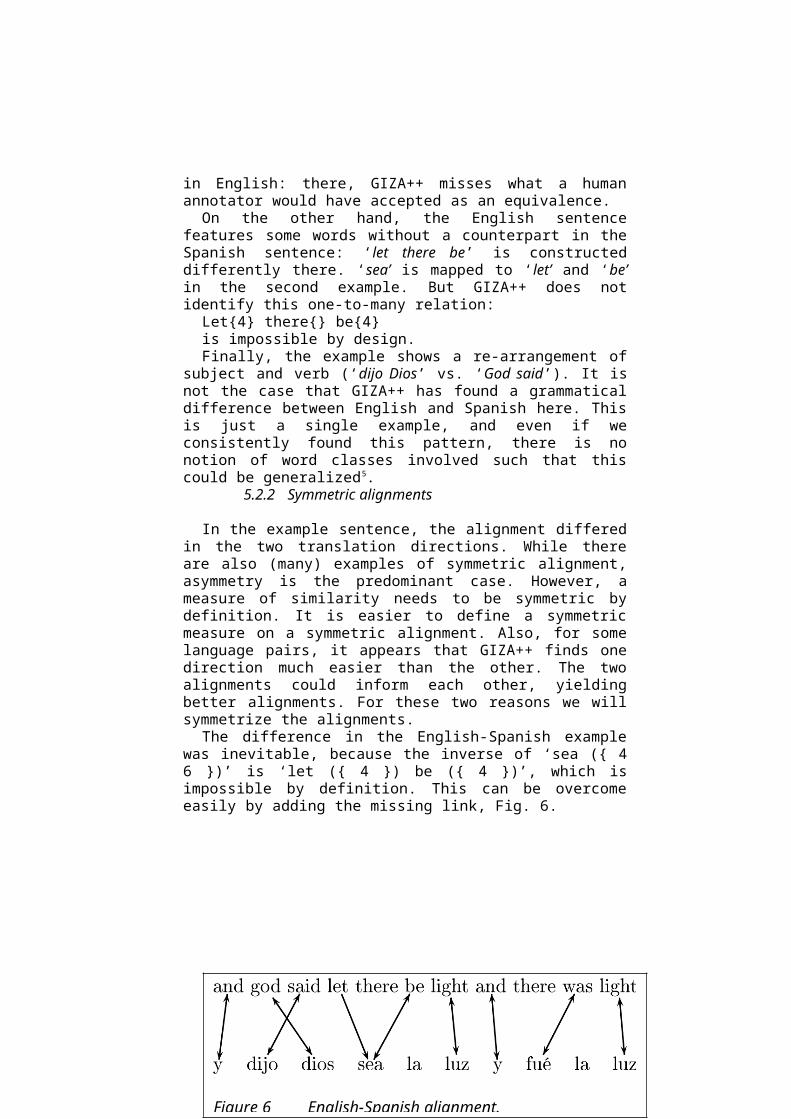
and god said let there be light and there was light NULL ({ 5 9 }) y ({ 1 }) dijo ({ 3 }) dios ({ 2 }) sea ({ 4 6 }) la ({ }) luz ({ 7 }) y ({ 8 }) fué ({ 10 }) la ({ }) luz ({ 11 })

NULL serves as an anchor for all non-alignable words, representing deletions. Being not aligned either is due to a structural difference between the two languages or to inconclusive evidence for GIZA++'s algorithm. The article la is not aligned, because in this construction English treats light as a mass noun, so there is no article. In other cases, articles are aligned non-consistently because of a wide range of possible articles in one language and only one definite article (the) in English: there, GIZA++ misses what a human annotator would have accepted as an equivalence.

On the other hand, the English sentence features some words without a counterpart in the Spanish sentence: ‘let there be’ is constructed differently there. ‘sea’ is mapped to ‘let’ and ‘be’ in the second example. But GIZA++ does not identify this one-to-many relation:

Let{4} there{} be{4}is impossible by design.Finally, the example shows a re-arrangement of subject and verb (‘dijo

Dios’ vs. ‘God said’). It is not the case that GIZA++ has found a grammat-ical difference between English and Spanish here. This is just a single ex-ample, and even if we consistently found this pattern, there is no notion of word classes involved such that this could be generalized5.

5.2.2 Symmetric alignments

In the example sentence, the alignment differed in the two translation directions. While there are also (many) examples of symmetric alignment, asymmetry is the predominant case. However, a measure of similarity needs to be symmetric by definition. It is easier to define a symmetric mea-sure on a symmetric alignment. Also, for some language pairs, it appears that GIZA++ finds one direction much easier than the other. The two align-ments could inform each other, yielding better alignments. For these two reasons we will symmetrize the alignments.

The difference in the English-Spanish example was inevitable, because the inverse of ‘sea ({ 4 6 })’ is ‘let ({ 4 }) be ({ 4 })’, which is impossible by definition. This can be overcome easily by adding the missing link, Fig. 6.

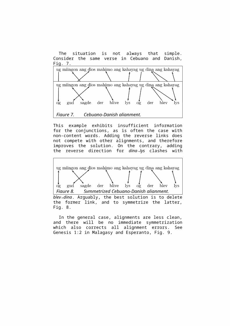
The situation is not always that simple. Consider the same verse in Ce-buano and Danish, Fig. 7.

Figure 6 English-Spanish alignment.

This example exhibits insufficient information for the conjunctions, as is often the case with non-content words. Adding the reverse links does not compete with other alignments, and therefore improves the solution. On the contrary, adding the reverse direction for dina→lys clashes with blev→dina. Arguably, the best solution is to delete the former link, and to symmetrize the latter, Fig. 8.

In the general case, alignments are less clean, and there will be no im-mediate symmetrization which also corrects all alignment errors. See Gen-esis 1:2 in Malagasy and Esperanto, Fig. 9.

We would like to achieve symmetrization nonetheless, and therefore de-vise a general strategy. If two words are mutually linked, or not linked at all, no action needs to be taken, as this is already symmetric. Every unidi-rectional link is either to be deleted or to be turned into a bidirectional one. A simple criterion shall decide: Keep the link if and only if it is the only one to connect (at least) one of the words involved. This minimizes un-aligned as well as multiply aligned words, which is meant to capture the intuition that one-to-one alignments are linguistically desirable (as also un-derlies GIZA++). It leads to the above mentioned correction of the Ce-

Figure 6. Cebuano-Danish alignment.Figure 7. Cebuano-Danish alignment.

Figure 8. Symmetrized Cebuano-Danish alignment.

buano-Danish example. For the other example, the result is much less

chaotic and linguistically more sound, Fig. 10.In the latter example, a certain notion of transitivity is violated because

both instances of "ny" do not connect with "super" although indirectly they are connected (disregarding the fact that this alignment is linguistically un-desired; as usual, GIZA++ has difficulties with articles). Other criteria when to keep a link and when to delete it might resolve this situation (and others) differently. For the present purposes, the one described above suf-fices.

5.3 Constructing similarity matrix

Maximal similarity is achieved by a non-crossing, one-to-one alignment of words. This is hardly ever the case, but it does appear (9989 out of approx-imately 31,102 sentence pairs for 37 languages, that is 0.048

For any possible measure, any alignment deviating from this ideal situa-tion has to receive a lower similarity value. In the general case, an align-ment is a permutation including insertions and deletions.

In the following, we consider two types of alignment measures. First, there are FEATURE-BASED measures (section 4.3.1). They count subse-quences or other properties shared by the two sentences. Typically, they are PARTIAL and often also LOCAL: they look at only a subset of the possible subsequences, say, subsequences bounded by a certain length. For these reasons, they are computationally efficient, yet they do not allow an inter-pretation of how one sentence would need to be re-ordered and modified in

Figure 9. Malagasy-Esperanto alignment.

Figure 10. Symmetrized Malagasy-Esperanto alignment.

order to obtain its translation. This is addressed by the second type of simi-larity measure we are considering: EDIT DISTANCE measures (section 4.3.2). They define a set of operations admissible to transform a sentence into another one. The minimal number of operations necessary then is the distance between two sentences, and distances can be converted into simi-larities.

For any measure, we take the average over all sentences as the overall similarity of two languages.

5.3.1 A feature-based measure

Let sentence similarity be defined as the number of shared bigrams, nor-malized by sentence length (minus 1) 6. Consider the above symmetric Malagasy-Esperanto example, in the notation of GIZA++, with Esperanto as the target, and without the actual words:

({ 1 }) ({ }) ({ 3 }) ({ 6 }) ({ 5,7,8 }) ({ 10 }) ({ 9 }) ({ 10 }) ({ 11 }) ({ 18 }) ({ 18 }) ({ }) ({ 14 }) ({ 15 }) ({ }) ({ 17 }) ({ }) ({ 17 }) ({ 13,18,19 }) ({ 18 }) ({ }) ({ 20 })

Count a shared bigram whenever two subsequent words in the target language appear in the same order as in the source language. The third and fourth word, aligned to words 3 and 6, respectively, are an example. We will skip non-aligned words. This has the effect that for example the first and third word form a bigram, which otherwise would be interrupted by the non-aligned article in both languages. Therefore the measure is one of per-mutation, and only indirectly one of insertions and deletions; they only come into play as missed chances of shared bigrams.

For multiply aligned words, evaluate the last alignment of the first and the first alignment of the last. Hence, ({ 6 }) ({ 5,7,8 }) is not a shared bi -gram, but ({ 5,7,8 }) ({ 10 }) is.

Altogether, there are 9 shared bigrams in 22 words in the example. The alignment similarity is computed as 9/(22-1)=0,429. 1 is subtracted from the sentence length because there are n-1 shared bigrams in a perfectly aligned sentence pair (see above). The reverse similarity (Malagasy as the target) is 14/(20-1)=0.739, which goes to show that feature-based measures will (possibly) yield different values depending on the direction, which means that they will also work on asymmetric alignments. In the strict sense then, this is not a similarity measure. It could be turned into one by taking the average of the two distances.

5.3.2 Edit distance

Assume that the source sentence is numbered 1 to l s, where ls is its length. Then the target sentence is obtained by the following operations:

- Deletion: Leaving a source word un-aligned.- Insertion: The reverse of deletion, introducing an un-aligned word

in the target language.- Split: Mapping one source word to many target words.- Merge: The reverse of split, mapping many words to one in the tar-

get.- Move: Displacing a word.The order of operations is nearly arbitrary, yet we want to restrict

merges to adjacent words, so (certain) moves have to happen beforehand. There exists a wealth of edit and permutation distances, (Deza & Deza

2009, ch. 11), yet there is none capturing splits and merges. They could be modelled as insertions and deletions of the surplus words, but this does not reflect the nature of the alignment: First, it could not serve as a description of the translation process. Second, there is no way to assign different weights to multi-word translations and real insertions. Third, discontinuous translations (see ({ 5,7,8 }) in the above example) will not be considered any more complex than continuous ones. For these reasons, we opt to treat splits and merges as primary operations, just as insertions and deletions. For similar reasons, a move should not be considered a combination of a deletion (in one place) and an insertion (in the other place). This motivates the need for 5 operations.

For the sake of transparency, we will only consider symmetric align-ments, obtained as outlined above (Section 5.2.2). The operations are sym-metric, so the measure is symmetric. Deletions and insertions, as well as merges and splits, can be treated alike: they are simply counted, and incur a unit cost of 1. The more problematic case is move. Coming from both sides of the translation, having performed all other four operations, we are left with a permutation problem. The above example reduces to the follow-ing:

1, 3, 6, 5, 7, 8, 10a, 9, 10b, 11, 18a, 18b, 14, 15, 17a, 17b, 13, 18c, 19, 18d, 20

as a permutation of:

1, 3, 5, 6, 7, 8, 9, 10a, 10b, 11, 13, 14, 15, 17a, 17b, 18a, 18b, 18c, 18d, 19, 20

The number of moves necessary is defined by the Ulam metric (see Deza & Deza, 2009, p. 212). Each move also incurs a unit cost. Together with the other operations, this is our definition of edit distance for align-ments. It is normalized for combined sentence length (i.e. divided by length(source) + length(target)), and subtracted from 1 in order to turn it into a similarity measure7.

5.4 Results

We clustered the 37 languages8 with CLANS and inspected the results manually. There are differences between the results using each of the two similarity measures, but none of them appear noteworthy.

Initial results closely resemble known language relationships. The Dra-vidian languages (Tamil, Telugu, Kannada) form a tight cluster, which cu-riously accomodates the otherwise isolate Korean as an outlier. Hebrew and Arabic (both Semitic; with Xhosa as a curious outlier), Danish and Norwegian, Cebuano and Tagalog (both Central Philippine), as well as Russian and Ukrainian feature close relations, see Fig. 12 and 13.

Resulting from the data sample European (Western Indo-European) lan-guages from the core cluster. Other language families are represented by only a few, one, or no data points at all. The Germanic languages exhibit a western (German, Dutch) and a nothern (Danish, Norwegian) subgroup, connected via Esperanto to the Romance languages: Spanish, Portuguese, French with Romanian as an outlier, and Italian, which is best connection for Albanian. Because of the geographic proximity this is an interesting point for further research9.

Figure 12. Clustering of Bible translations: Overall picture

Figure 13. Clustering of Bible translations: Main cluster

These western European languages further connect to the group of Slavic languages, which are more loosely inter-connected. The remaining languages either appear as isolates or as near-isolates with no conclusive connections. A larger Malayo-Polynesian group (the two Central Philip-pine languages plus Maori, Indonesian, and Malagasy) cannot be estab-lished.

English plays a literally central role. It lies inmidst the above mentioned European groups. Many languages are only kept within the core cluster be-cause they enjoy a strong link to English. This is true of at least Persian, Maori, Chinese, Somali, Hindi, and Indonesian. We suspect these transla-tions might be based on an English one (or maybe on the Latin Vulgate, to which the English translation is very close). In the case of Maori, it is rea-sonable to assume that the translator was a native speaker of English. In or-der to clean up the picture, we additionally clustered all languages except English. In this run, for example, Cebuano and Tagalog separate from the core of European languages well before, say, the Slavic languages.

5.4.1 Intra- versus inter-language variation

Language duplicates were excluded from the above reported experiments. In another clustering, we specifically looked at intra-language variation. The lowest similarity value for two English translations (edit distance mea-sure) is 0.78, while it goes as high as 0.99 (King James Version vs. Web-ster's Revised King James Version). Despite this internal variation, English forms a tight cluster, with the most diverging versions as outliers. The cut-off in CLANS can safely be set higher; these two do not need to be directly connected. 0.8 is a reasonable value, because the two German and Spanish version rate at 0.82 and 0.85, respectively. These values are otherwise only reached by Arabic and Hebrew (0.82) and Norwegian and Danish (0.80; this Norwegian Bible (in Bokmål) is apparently a translation from Dan-ish10). Some other language pairs (Dutch-English, Esperanto-English) ex-ceed or get close to the threshold of 0.78, but only in comparison with out-liers of the English group. Overall, there will be a lower similarity be-tween, say, Dutch and English.

Other significant similarities are Dutch-German and Spanish-Por-tuguese (0.78 each, considering the better match of the languages with two versions available), and other closely related languages. Similarities below 0.8 are fairly evenly distributed, with no apparent gaps. Altogether there is

small overlap between the similarities of identical and closely related lan-guages, so the method cannot always keep them apart. It comes as no sur-prise that Danish and Norwegian, notably Bokmål and not Nynorsk, and considering the conservative language used in Bible translations, cannot be kept apart on a syntactic level more than needs to be allowed for as intra-language variation. The method proves to be reasonable in the sense that intra-language variation is smaller than inter-language variation11, and the inevitable border cases are interpretable as such.

In conclusion, our methods adds a robust and fully automatic measure of linguistics similarity to the existing ones. This helps in refining the ge-nealogy of languages and in identifying features shared not because of a common origin, but because of language contact.

6 Conclusion

In this paper, we have argued for the introduction of a clustering approach into the study of language relationships. Potentially, it might be able to take into account both phylogenetic and contact-induced signals.

It goes without saying that the approach advocated here is called to sup-plement, and not supplant, the classical techniques of historical linguistics. We consider it as a source of hints for historical linguists as to which path of inquiry might be worth pursuing.

We have shown that using CLANS allows to roughly reproduce known genetic units. This can be achieved with a relatively small amount of man-ual curation.

Furthermore, we have argued that although the use of traditional “overt” morphosyntactic features does not allow to even remotely reproduce known genetic classification, a promising alternative comes from auto-mated text alignment. Unfortunately, creating a sufficiently representative aligned corpus remains prohibitively effort-consuming.

Clustering approaches are particularly efficient at analyzing large sets of data. If the dream of large scale language classification is ever to come true, the comparison of huge amounts of data is an inevitable step. We hope that clustering approaches will play a significant role in this en-deavor.

Notes

1. An exception is the Neighbor Joining Method (Saitou and Nei 1986), which is cubic in the number of points. However, trees it produces are considered less accurate.

2. We thank the authors for sharing their database with us.3. We thank Soeren Wichmann for sharing the database with us.4. http://www.biblegateway.com/versions/; http://www.jesus.org.uk/bible5. GIZA++ can be provided with word class information to improve align-

ments, but even then it does not directly discover grammatical rules.6. When the sentence length equals one, we can posit that the function equals

1. The number of such sentences in the corpus is so low, that it does not af -fect any conclusions.

7. There are alternative possibilities here.8. Those with several instances were represented by a single translation, in or-

der to reduce the (quadratic) computational effort.9. Unfortunately, the source (http://www.biblegateway.com/versions/in-

dex.php?action=getVersionInfo&vid=1) does not say anything about the ori-gin of this translation.

10. http://no.wikipedia.org/wiki/Det_Norske_Bibelselskap11. The small sample does not allow for testing for significance.

References

Campbell, Lyle; Poser, William J.2008 Language Classification: History and Method. Cambridge Univer-

sity PressDeza, Michel Marie, and Deza, Elena.

2009 Encyclopedia of Distances. Berlin et al: Springer.Donohue, Mark, Simon Musgrave, Bronwen Whitting, and Søren Wichmann

2011 Typological feature analysis models linguistic geography. Lan-guage 87.2: 369-383.

Dunn, Michael 2009 Contact and phylogeny in Island Melanesia. Lingua, 11(11), 1664-

1678.Dunn, Michael, Levinson, S. C., Lindström, E., Reesink, G., & Terrill, A.

2008 Structural phylogeny in historical linguistics: Methodological ex-plorations applied in Island Melanesia. Language, 84(4), 710-759.

Dyen, Isidore, Kruskal Joseph B., and Black, Paul1992 An Indoeuropean Classification: A Lexicostatistical Experiment.

Transactions of the American Philosophical Society. New Series, Vol. 82, No. 5.

Forster, Peter and Renfrew, Colin (eds.)2006 Phylogenetic methods and the prehistory of languages.

Frickey, Tancred and Andrei Lupas 2004 Clans: a java application for visualizing protein families based on

pairwise similarity. Bioinformatics, 20(18):3702-3704.Fruchterman, Thomas M. J.; Reingold, Edward M.

1991 Graph Drawing by Force-Directed Placement. Software – Practice & Experience (Wiley) 21 (11): 1129–1164.

Gray, Russell D. and Atkinson, Quentin D.2003 Language-tree divergence times support the Anatolian theory of

Indo-European origin. Nature 426, 435-439.Greenberg, Joseph

1987 Language in the Americas. Stanford, CA: Stanford University Press.

Greenhill, Simon; Atkinson, Quentin; Meade, Andrew and Gray, Russel D.2011 The shape and tempo of language evolution. Proceedings of the

Royal Society. Series B. 278:474-479Haspelmath, Martin, Dryer Matthew S., Gil, David and Comrie, Bernard, eds.

2008 The World Atlas of Language Structures Online. Munich: Max Planck Digital Library.

Huson, Daniel and Bryant, David 2006 Application of Phylogenetic Networks in Evolutionary Studies,

Molecular biology and evolution., 23(2):254-267Langobardi, Giuseppe, Guardiano, Christina

2009 Evidence for syntax as a signal of historical relatedness. Lingua 119, (11), 1679-1706

Nichols, Johanna and Warnow, Tandy

2008 Tutorial on Computational Linguistic Phylogeny. Language and Linguistics Compass Vol. 2(5), p. 760–820. Och, Franz Josef and Ney, Hermann

2003 A Systematic Comparison of Various Statistical Alignment ModelsComputational Linguistics, vol. 29(1), pp. 19--51

Petroni, Philippo and Serva, Maurizio

2010 Measures of lexical distance between languages. Physica A: Statis-tical Mechanics and its Applications. 389(11), 2280-2283

Resnik, Philip; Broman Olsen, Mari and Mona Diab1999 The Bible as a Parallel Corpus: Annotating the ‘Book of 2000

Tongues’, Computers and the Humanities, 33(1--2), pp. 129--153,.Saitou, Naruya and Nei, Masatoshi

1987 The neighbor-joining method: A new method for reconstructing phylogenetic trees. Molecular biology and evolution. 4(4): 406-425.

Wichmann, Søren, Holman, Eric W., Bakker, Dik, Brown, Cecil H.2010 Evaluating linguistic distance measures. Physica A 389, 3632-363