Monitoring of steel-lined pressure shafts using water-hammer records and wavelet filtering and decomposition

F.H. Hachem1 and A.J. Schleiss1

1Laboratory of Hydraulic Constructions (LCH) Ecole Polytechnique Fédérale de Lausanne (EPFL)

Station 18, 1015 Lausanne SWITZERLAND

E-mail: fadi.hachem@epfl.ch

Abstract: The failure of steel liner of pressure shafts of hydropower plants can have catastrophic consequences. The partial or total loss of the liner support’s rigidity is characterized by a local change of the hydro-acoustic properties and creates reflection boundaries for the water waves. This paper presents a new monitoring method for detecting and locating weak reaches by processing reflected water-hammer waves at the boundaries of the shaft. These water-hammers are generated experimentally by a shut-off valve installed at the downstream end of a test pipe. The weak reaches are modeled by replacing the steel of the pipe’s wall with aluminum and PVC materials. Different test pipe configurations are created by changing the position of these reaches along the test pipe. The monitoring procedure uses the Fast Fourier Transform and wavelet decomposition techniques to estimate the incident-reflection travel time between the pressure sensors and the weak reaches boundaries. Keywords: Steel-lined pressure tunnels and shafts, pipe wall stiffness, water-hammer, wavelet decomposition, weak reaches, wave reflection, transient flow.

1. INTRODUCTION

One of the multiple objectives of the so called HydroNet research project (Modern methodologies for the design, manufacturing and operation of pumped-storage plants) is the creation and enhancement of new non-intrusive monitoring methods for steel-lined pressure shafts and tunnels. The idea is to assess records of the dynamic water pressure acquired during the water-hammer phenomena in purpose to identify the existence and location of a weak reach. This latter is generated by the local structural deterioration of the backfill concrete and/or the rock mass surrounding the liner. This reduces the overall wave speed and creates reflection boundaries for the incident pressure waves. From the state-of-the-art review, it can be concluded that there is a large number of techniques that deal with faults in pipelines such as leak detection (Ferrante & Brunone, 2002, Covas et al., 2005, Wang et al., 2005, Lee et al., 2005, Shamloo & Haghighi, 2009, Taghvaei et al., 2010, etc). In all these methods, the pressure wave speed is assumed to be a constant value throughout the pipeline length. A different structural wall aspect has been studied by Stephens (2008) to estimate the location of internal damage wall of a composite concrete-steel pipeline based on transient model combined with a Genetic Algorithm and field measurements. The herein paper investigates experimentally the alteration of the water-hammer wave speed in presence of local weak reaches (that have different hydro-acoustic parameters) and assesses wave reflections inside a test pipe. Under an axi-symmetrical behavior, the multilayer system (steel–concrete–rock) of the pressurized shaft can be modeled by one layer system of a steel test pipe which is divided into several reaches. The weak reach is simulated by exchanging the steel reach with an aluminum or PVC material. To detect the longitudinal stiffness heterogeneity, different geometric configurations of the steel test pipe were examined experimentally by changing systematically the position of an aluminum and PVC pipe reach of 50 cm length. For the estimation of the wave speed and the prediction of the incident–reflection travel time between the weak reach boundaries and the pressure sensors, the Fast Fourier Transform, the cross-correlation technique and the wavelet filtering and decomposition methods were applied on the pressure data records at the both end of the test pipe.

10th Hydraulics Conference33rd Hydrology & Water Resources Symposium34th IAHR World Congress - Balance and Uncertainty 26 June - 1 July 2011, Brisbane, Australia

ISBN 978-0-85825-868-6 Engineers Australia2289

2. THEORY

2.1. Water-hammer

When water flow in pressurized waterways (pipes, tunnels and shafts) is suddenly stopped, pressure waves, known as water-hammer, are generated according to the acoustic plane wave equation written as follows (Parmakian, 1963 and Bergant et al., 2008):

∂ ∂ ∂− = −∂ ∂ ∂

2 2

2 2 2

vh g h vg fx a t D x

(1)

where, h(x,t) is the piezometric head, v(x,t) is the water flow velocity, t is the time, x is the longitudinal dimension, g is the acceleration due to gravity, a is the speed of sound in water or the pressure wave velocity, f is the Darcy–Weisbach friction factor and D is the internal diameter of the waterway. These waves travel along the waterway until they hit the borders (or junction) of a reach having different hydro-acoustic properties (different flow area and/or pressure wave velocity) from the rest of the waterway. At these boundaries, the waves are partly transmitted and partly reflected back towards the source. For steel-lined pressure tunnels, such a different hydro-acoustic reach may exist when a decrease of the wave speed appears due to a partial or total loss of the stiffness of the exterior support of the steel liner which is provided by the surrounding backfill concrete and rock mass. This reach with a wave speed lower than the rest of the tunnel is called ‘’weak reach’’ throughout this paper.

p1 p2

Shut-off Valve

Air vessel

1x

Weak reach

2x

(a)

(b) (c)

Nor

mal

ized

hea

d @

p2

Nor

mal

ized

hea

d @

p1

Junction 2

x 5.52·10-3, Time [s]

t1 Reflection from the weak reach

t2

tup

tdown

Junction 1

Figure 1 a) Schematic view of the test pipe, b) the normalized head at the pressure sensor p2 obtained from numerical calculation, and c) the normalized head at the pressure sensor p1 of

the same numerical model

Figure 1a shows a schematic longitudinal profile of the test pipe with a weak reach having boundaries situated at distances x1 and x2 from the pressure sensor p2. This weak reach has a wave speed value a2 lower than the rest of the test pipe (a1). An incident pressure wave of magnitude (hi-h0) coming from the shut-off valve is divided into transmitted and reflected waves when crossing junction 1. For a uniform cross-section flow area and a frictionless pipe, the magnitude of the transmitted wave (ht1-h0) is given by (Wylie et al., 1993):

( )− = −+

1 0 01

2

2

1t ih h h ha

a

(2)

2290

where, h0, hi and ht1 are the steady-state, incident and transmitted piezometric heads, respectively. The same phenomenon is reproduced when the pressure wave crosses the downstream end of the weak reach (junction 2). According to the direction of the first incident wave hi , junctions 1 and 2 are called the upstream and downstream ends of the weak reach. Figures 1b and 1c show the normalized pressure records p1 and p2 obtained from a numerical calculation that uses the method of characteristic to solve Eqs. (1) and (2). In these numerical results, the pressure reflections from the boundaries of the weak reach can be easily identified by the pressure drop shown on Figure 1b. The value of the mean wave speed (amean) can be extracted by dividing the known distance separating the two pressure sensors by the predicted travel time (t1-t2). The incident-reflection travel times from the boundaries of the weak reach (tup and tdown) can be clearly identified on Figure 1b. The weak reach can then be located by the two longitudinal coordinates x1 and x2 as follows:

,1,2 2

mean up downa tx

⋅= (3)

In plain strain conditions and considering the hypothesis of linear elasticity and small deformations, the wave velocity can be estimated by the following formula (Halliwell, 1963):

11 2 d ( )

d

sr

ww i

au r

K r p

=⎛ ⎞

ρ + ⋅⎜ ⎟⎝ ⎠

(4)

in which d ( )

d

sru rp

is the first derivative of the radial displacement of the steel liner urs relative to the

internal pressure p at the water–liner interface of radius ri. The d ( )d

sru rp

ratio is nothing else than the

inverse of the radial stiffness of the tunnel wall. By ignoring the presence of air in water, the velocity of a pressure wave travelling between two cross-sections of a tunnel will be affected by every change of the radial stiffness of its wall. In the laboratory tests, the change of the wall stiffness is modeled by using pipe reaches having different (E·e) values than the rest of the test pipe. E is the Young modulus and e is the thickness of the pipe wall.

2.2. Signal processing

The signal processing is needed to assess the experimental data which are more difficult to analyse than the numerical results shown on Figures 1b and 1c. This is mainly due to the presence of noise and to the wave dispersion and attenuation phenomena. The processing of experimental pressure signals p1 and p2 is done using the filtering and decomposition techniques of wavelets (Mallat, 1990). The main advantage provided by such a technique is its ability to de-noise the signal without significant degradation and distortion. Similar to the Fourier transform which uses sine waves of various frequencies as basis, wavelet analysis is the breaking up of the signal into shifted and scaled versions of the original (or mother) wavelet. The wavelet transform provides coefficients C(λ,u) that represent a sort of correlation degree between the wavelet, scaled to λ, and the section of the signal at time u. The wavelet coefficient expression for a signal p(t) can be written as follows:

−⎛ ⎞λ = ψ ⎜ ⎟λλ ⎝ ⎠∫1( , ) ( ) t uC u p t dt (5)

where, λ and u are the dilation or scale, and the translation parameter, respectively. Ψ(λ,u) are the transform basis functions or wavelets. The wavelet coefficients and basis functions are then used to decompose the signal into a hierarchical set of so called approximations and details. At each decomposition level j, the signal is passed through a pair of high-pass and low-pass filters. The details coefficients are the result of the former filter while the approximation coefficients are those obtained

2291

from the latter one. The detail coefficient Dj at level j is given by the following equation (The Mathworks Inc., 2008):

∈

−⎛ ⎞= ⋅ ψ ⎜ ⎟⎝ ⎠

∑ 1( ) ( , )jk

t kD t C j kjj (6)

where, λ = 2 j and = ⋅2ju k with k as the time index. After J levels of decomposition, the original pressure signal p(t) can be expressed as:

= > == + = +∑ ∑ ∑

1 1( ) ( ) ( ) ( ) ( )

J J

J j j jj j J j

p t A t D t D t D t (7)

where, AJ is the approximation coefficients. The wavelet technique is used within this paper as a band-pass filter for the measured pressure signals.

3. EXPERIMENTS

3.1. Description of the experimental set-up

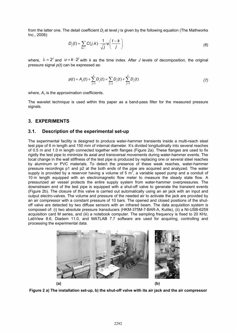
The experimental facility is designed to produce water-hammer transients inside a multi-reach steel test pipe of 6 m length and 150 mm of internal diameter. It’s divided longitudinally into several reaches of 0.5 m and 1.0 m length connected together with flanges (Figure 2a). These flanges are used to fix rigidly the test pipe to minimize its axial and transversal movements during water-hammer events. The local change in the wall stiffness of the test pipe is produced by replacing one or several steel reaches by aluminum or PVC materials. To detect the presence of these weak reaches, water-hammer pressure recordings p1 and p2 at the both ends of the pipe are acquired and analyzed. The water supply is provided by a reservoir having a volume of 5 m3, a variable speed pump and a conduit of 10 m length equipped with an electromagnetic flow meter to measure the steady state flow. A pressurized air vessel protects the entire supply system from water-hammer overpressures. The downstream end of the test pipe is equipped with a shut-off valve to generate the transient events (Figure 2b). The closure of this valve is carried out automatically using an air jack with an input and output electro-valves. The volume and pressure of the needed air to activate the jack are provided by an air compressor with a constant pressure of 10 bars. The opened and closed positions of the shut-off valve are detected by two diffuse sensors with an infrared beam. The data acquisition system is composed of: (i) two absolute pressure transducers (HKM-375M-7-BAR-A, Kulite), (ii) a NI-USB-6259 acquisition card M series, and (iii) a notebook computer. The sampling frequency is fixed to 20 KHz. LabView 8.6, Diadem 11.0, and MATLAB 7.7 software are used for acquiring, controlling and processing the experimental data.

(a) (b)

Figure 2 a) The installation set-up, b) the shut-off valve with its air jack and the air compressor

2292

3.2. Test pipe configurations

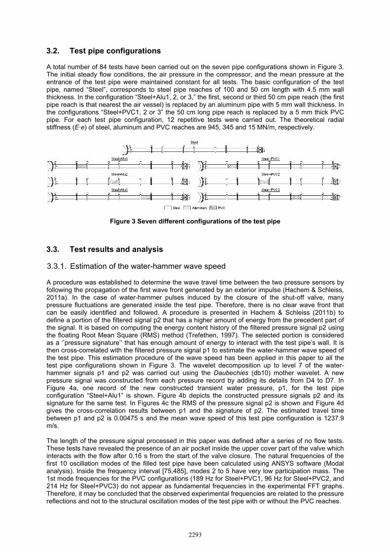
A total number of 84 tests have been carried out on the seven pipe configurations shown in Figure 3. The initial steady flow conditions, the air pressure in the compressor, and the mean pressure at the entrance of the test pipe were maintained constant for all tests. The basic configuration of the test pipe, named “Steel”, corresponds to steel pipe reaches of 100 and 50 cm length with 4.5 mm wall thickness. In the configuration “Steel+Alu1, 2, or 3,” the first, second or third 50 cm pipe reach (the first pipe reach is that nearest the air vessel) is replaced by an aluminum pipe with 5 mm wall thickness. In the configurations “Steel+PVC1, 2 or 3” the 50 cm long pipe reach is replaced by a 5 mm thick PVC pipe. For each test pipe configuration, 12 repetitive tests were carried out. The theoretical radial stiffness (E·e) of steel, aluminum and PVC reaches are 945, 345 and 15 MN/m, respectively.

Figure 3 Seven different configurations of the test pipe

3.3. Test results and analysis

3.3.1. Estimation of the water-hammer wave speed

A procedure was established to determine the wave travel time between the two pressure sensors by following the propagation of the first wave front generated by an exterior impulse (Hachem & Schleiss, 2011a). In the case of water-hammer pulses induced by the closure of the shut-off valve, many pressure fluctuations are generated inside the test pipe. Therefore, there is no clear wave front that can be easily identified and followed. A procedure is presented in Hachem & Schleiss (2011b) to define a portion of the filtered signal p2 that has a higher amount of energy from the precedent part of the signal. It is based on computing the energy content history of the filtered pressure signal p2 using the floating Root Mean Square (RMS) method (Trefethen, 1997). The selected portion is considered as a ‘’pressure signature’’ that has enough amount of energy to interact with the test pipe’s wall. It is then cross-correlated with the filtered pressure signal p1 to estimate the water-hammer wave speed of the test pipe. This estimation procedure of the wave speed has been applied in this paper to all the test pipe configurations shown in Figure 3. The wavelet decomposition up to level 7 of the water-hammer signals p1 and p2 was carried out using the Daubechies (db10) mother wavelet. A new pressure signal was constructed from each pressure record by adding its details from D4 to D7. In Figure 4a, one record of the new constructed transient water pressure, p1, for the test pipe configuration “Steel+Alu1” is shown. Figure 4b depicts the constructed pressure signals p2 and its signature for the same test. In Figures 4c the RMS of the pressure signal p2 is shown and Figure 4d gives the cross-correlation results between p1 and the signature of p2. The estimated travel time between p1 and p2 is 0.00475 s and the mean wave speed of this test pipe configuration is 1237.9 m/s. The length of the pressure signal processed in this paper was defined after a series of no flow tests. These tests have revealed the presence of an air pocket inside the upper cover part of the valve which interacts with the flow after 0.16 s from the start of the valve closure. The natural frequencies of the first 10 oscillation modes of the filled test pipe have been calculated using ANSYS software (Modal analysis). Inside the frequency interval [75,485], modes 2 to 5 have very low participation mass. The 1st mode frequencies for the PVC configurations (189 Hz for Steel+PVC1, 96 Hz for Steel+PVC2, and 214 Hz for Steel+PVC3) do not appear as fundamental frequencies in the experimental FFT graphs. Therefore, it may be concluded that the observed experimental frequencies are related to the pressure reflections and not to the structural oscillation modes of the test pipe with or without the PVC reaches.

2293

(a) (b)

(c) (d)

Figure 4 a) Constructed pressure signal p1, b) Constructed pressure signal p2 and its signature, c) the RMS of the constructed pressure p2, and c) the cross-correlation results

between pressure p1 and the signature of pressure p2

The estimated values of the water-hammer wave speed for all the pipe configurations are shown in Figure 5 with their means and standard deviations evaluated for each pipe configuration. The theoretical values computed from Eq. (4) are also shown. The change of the means of the wave speed indicates the presence of a local weak reach in the test pipe. The relative differences between these means are proportional to the severity of the stiffness change. No clear differences can be observed for the “Steel+Alu” configurations. For all the pipe configurations, the mean measured wave speed is smaller than the theoretical one. The relative differences between the measured and theoretical speeds are 3.6, 3.9, and 14.9% for the “Steel”, “Steel+Alus”, and “Steel+PVCs” configurations, respectively. The small differences for the two former pipe configurations can be explained by the fact that the quasi-steady and the unsteady shear stress between the flow and the pipe wall are ignored in Eq. (4). The additional differences in “Steel+PVCs” configurations could results from the wave reflection and transmission phenomena at weak reach boundaries and/or from the visco-elastic behavior of the PVC reach.

900

1000

1100

1200

1300

1400

0 5 10 15 20 25 30 35 40 45 50 55 60 65 70 75 80 85

Wat

er-h

amm

er w

ave

spee

d [m

/s]

Test number

Steel Stee+Alu1Steel+Alu2 Steel+Alu3Steel+PVC1 Steel+PVC2Steel+PVC3 MeanMean+Std Mean-StdTheo. speed (Eq. (4))

Figure 5 Estimated water-hammer wave speed; mean values and standard deviations for the 84

tests carried out on seven pipe configurations

Pre

ssur

e, p

1 [b

ar]

Pre

ssur

e, p

2 [b

ar]

Time [s] Time [s]

RM

S o

f the

pre

ssur

e si

gnal

p2

[bar

]

Cro

ss-C

orre

latio

n co

effic

ient

[-]

Time [s] Time [s]

2294

3.3.2. Locating of the weak reach

The incident-reflection travel times, tup and tdown, are estimated by the Fast Fourier Transform (FFT with Hanning windowing) of the 12 constructed pressure records p1 and p2 carried out for each test pipe configuration. The FFT records of the test configurations with Aluminum reach are very similar to those for “Steel” configuration. Therefore, the localization of such reaches using the FFTs approach is not possible. For the configurations with PVC weak reach, the mean of the normalized FFT (RMS amplitude) for p1 and p2 is computed. The normalization is done by dividing the FFT magnitudes by the one at 80 Hz. This frequency corresponds to the incident-reflection travel time between the supply reservoir and the air vessel. Figures 6 show the average curves of the normalized FFT for the “Steel” and “Steel+PVC1” configurations. The identification of the frequency that corresponds to the weak reach for each pipe configuration is done after discarding the FFT peaks of the “Steel+PVCs” records that have the same frequencies as peaks of the “Steel” configuration. For the remaining peaks, a couple of peak frequencies composed by one FFT of p1 and one FFT of p2 peaks (indicated by circles in Figures 6), is chosen. The frequency fp1,p2 of the propagating wave between the upstream and downstream reservoirs is then estimated according to the following equation:

⋅

=+

max 1 max 21, 2

max 1 max 2

p pp p

p p

f ff

f f (8)

where fmax p1 and fmax p2 are the frequencies at the FFT maximum peak of p1 and p2, respectively. The frequencies fp1,p2 are then compared to the theoretical value obtained from the ratio asteel / (2·Lpipe) where asteel is the estimated wave speed of the “Steel” configuration (asteel=1245.4 m/s) and Lpipe is the total length of the test pipe between the two reservoir (Lpipe=8.25 m). The pair of frequencies which gives the nearest fp1,p2 frequency relative to the theoretical value is retained. Many samples of the steady-state pressure signals for each water-hammer test were analyzed in order to determine the noise level and the magnitudes of the FFT peaks caused by the pump. The signal-to-noise ratio varies between 3.4 and 340.2 and the FFT peaks magnitudes are below 0.0001. For “Steel+PVCs” configurations, this latter value is about 1.5 and 4.5 times lower than the mean FFT amplitude at 80 Hz of pressure p1 and p2, respectively.

0.0

0.5

1.0

1.5

2.0

2.5

3.0

75 125 175 225 275 325 375 425 475

Nor

m. F

FT fo

r pre

ssur

e p1

[-]

Frequency [Hz]

"Steel+PVC1"

330 Hz

0.0

0.5

1.0

1.5

2.0

2.5

75 125 175 225 275 325 375 425 475

Nor

m. F

FT fo

r pre

ssur

e p2

[-]

Frequency [Hz]

120 Hz

0.0

1.0

2.0

3.0

4.0

75 125 175 225 275 325 375 425 475

Nor

m. F

FT fo

r pre

ssur

e p1

[-]

Frequency [Hz]

"Steel"

0.0

0.4

0.8

1.2

75 125 175 225 275 325 375 425 475

Nor

m. F

FT fo

r pre

ssur

e p2

[-]

Frequency [Hz]

(a) (b)

Figure 6 Average FFT of the 12 tests of the “Steel” and “Steel+PVC1” pipe configuration. a) The FFT for the constructed pressure records p1 and b) the FFT for the constructed pressure

records p2

2295

By repeating the localization procedure for all the test pipe configurations with a PVC reach, it was possible to determine the approximate position of the weak reach. Figure 7 shows the estimated and the real center position of the weak reaches evaluated relative to the positions of sensors p1. The differences of the estimated weak reach location relative to the sensors distance of 5.88 m are also shown in the same figure. These differences are between 1.3% and -16.2%.

0.0 0.5 1.0 1.5 2.0 2.5 3.0 3.5 4.0 4.5 5.0 5.5 6.0

2

3

4

5

6

Estimated distances to the center of the pipe weak reaches measured from the pressure sensor position p1 [m]

Rea

ches

inde

xes

[-]

-20-15-10-505101520

2

3

4

5

6

Relative differences between the real and the estimated weak reaches position [%]

Figure 7 Estimated, real and relative differences of distances from the p1 sensor position to the center of the weak reach for the three PVCs tested configurations

4. CONCLUSIONS

An experimental facility which allows producing water-hammer inside a test pipe with reaches of different stiffness has been described. The results of a large number of tests carried out on seven test pipe configurations have been also analyzed. The wavelet technique was used to filter the dynamic pressure records and the cross-correlation method was applied to estimate the water-hammer wave speed for each pipe configuration. An important drop of the mean wave speed values estimated from the pressure measurements has been identified for configurations with PVC reaches. This drop was smaller when aluminum reaches were used. The position of the PVC reach used in the “Steel+PVCs” configurations has been also estimated using the FFT approach applied on pressure signals and the mean of the measured wave speeds for “Steel” test pipe. The differences in predicting the location of the center section of the weak reach relative to the distance separating the two pressure sensors are between 1.3% and 16.2%. The ongoing research will try to validate the estimation procedure of the water-hammer wave speed for other test pipe configurations. More analyses will enhance the methodology of localization of the weak reaches. In-situ dynamic pressure measurements at both ends of a pressure shaft of a pumped-storage power plant are ongoing. They will provide additional information about the steepness, energy and dissipation of water-hammer wave generated during start-up and shut-down of pumps and turbines. The influence of the water temperature, turbidity, and the captured air inside the shaft on the estimation of the wave speed will be also investigated. The localization procedure of weak reaches will be implemented in purpose to detect the position of some eventual geological and geotechnical weaknesses of the rock mass surrounding the steel liner. The estimated positions will be compared to the real geological weaker zones which can be obtained from the existing as-built drawings of the shaft.

5. ACKNOWLEDGMENTS

The study is part of the research project HydroNet for the design, manufacture and operation of pumped storage plants funded by the Swiss Competence Center Energy and Mobility (CCEM-CH), the Swiss Electrical Research and the Swiss Office for Energy.

2296

6. REFERENCES

ANSYS Mechanical, Release 12.0, ANSYS Inc, 2009. (www.ansys.com).

Bergant, A., Tijsseling, A., Vitkovsky, J., Covas, D., Simpson, A. and Lambert, M. (2008). Parameters affecting water-hammer wave attenuation, shape and timing—Part 1: Mathematical tools, Journal of Hydraulic Research, 46 (3), 373–381.

Covas, D., Ramos, H. and Betâmio de Almeida, A. (2005), Standing wave difference method for leak detection in pipeline systems, Journal of Hydraulic Engineering, 131 (12), 1106–1116.

Ferrante, M. and Brunone, B. (2002), Pipe system diagnosis and leak detection by unsteady-state tests. 2. Wavelet analysis, Advances in Water Resources, 26, 107–116.

Hachem, F.E. and Schleiss, A.J. (2011a), Detection of local wall stiffness drops in pipes using steep pressure wave excitation and wavelet decomposition, second round review in the Journal of Hydraulic Engineering, ASCE.

Hachem, F.E. and Schleiss, A.J. (2011b), Physical tests estimating the water-hammer wave speed in pipes and tunnels with local weak wall stiffness, Proceedings of the 2011 World Environmental & Water Resources Congress (EWRI), Palm Springs, California, May 22 – 26, 2011.

Halliwell, A.R. (1963). Velocity of a Waterhammer Wave in an Elastic Pipe, Journal of the Hydraulics Division, ASCE, 89 (HY4), 1–21.

Lee, P.J., Vitkovsky, J.P., Lambert, M.F., Simpson, A.R. and Liggett, J.A. (2005). Frequency Domain Analysis for Detecting Pipelines Leaks, Journal of Hydraulic Engineering, ASCE, 131 (7), 596-604.

Mallat, S.G. (1990). A Wavelet Tour of Signal Processing, Academic Press, San Diego, CA.

Parmakian, J. (1963), Waterhammer analysis, Dover, New York.

Stephens, M.L. (2008), Transient response analysis for fault detection and pipeline wall condition assessment in field water transmission and distribution pipelines and networks. Thesis submitted for the degree of Doctor of Philosophy, School of civil and environmental engineering, University of Adelaide, SA, South Australia.

Shamloo, H. and Haghighi, A. (2009), Leak detection in pipelines by inverse backward transient analysis, Journal of Hydraulic Research, 47 (3), 311-318.

Taghvaei, M., Beck, S.B.M. and Boxall, J.B. (2010), Leak detection in pipes using induced water hammer pulses and cepstrum analysis, International Journal of COMADEM , 13 (1), 19-25.

The Mathworks, Inc. (2008). MATLAB, Natick, Mass. (www.mathworks.com).

Trefethen, L.N. (1997), Numerical linear algebra. Society for Industrial and Applied Mathematics, Philadelphia.

Wang, X.J., Lambert, M.F. and Simpson, A.R. (2005). Detection and Location of a Partial Blockage in a Pipeline Using Damping of Fluid Transients, Journal of Water Resources Planning and Management, 131 (3), 244-249.

Wylie, E.B., Suo, L. and Streeter, V.L. (1993). Fluid Transients in Systems, facsimile edition, Prentice Hall, Englewood Cliffs, NJ.

2297