DI

SC

US

SI

ON

P

AP

ER

S

ER

IE

S

Forschungsinstitut zur Zukunft der ArbeitInstitute for the Study of Labor

Monitoring Job Offer Decisions, Punishments,Exit to Work, and Job Quality

IZA DP No. 4325

July 2009

Gerard J. van den BergJohan Vikström

Monitoring Job Offer Decisions,

Punishments, Exit to Work, and Job Quality

Gerard J. van den Berg VU University Amsterdam, IFAU Uppsala,

CEPR, IFS and IZA

Johan Vikström

Uppsala University and IFAU Uppsala

Discussion Paper No. 4325 July 2009

IZA

P.O. Box 7240 53072 Bonn

Germany

Phone: +49-228-3894-0 Fax: +49-228-3894-180

E-mail: iza@iza.org

Any opinions expressed here are those of the author(s) and not those of IZA. Research published in this series may include views on policy, but the institute itself takes no institutional policy positions. The Institute for the Study of Labor (IZA) in Bonn is a local and virtual international research center and a place of communication between science, politics and business. IZA is an independent nonprofit organization supported by Deutsche Post Foundation. The center is associated with the University of Bonn and offers a stimulating research environment through its international network, workshops and conferences, data service, project support, research visits and doctoral program. IZA engages in (i) original and internationally competitive research in all fields of labor economics, (ii) development of policy concepts, and (iii) dissemination of research results and concepts to the interested public. IZA Discussion Papers often represent preliminary work and are circulated to encourage discussion. Citation of such a paper should account for its provisional character. A revised version may be available directly from the author.

IZA Discussion Paper No. 4325 July 2009

ABSTRACT

Monitoring Job Offer Decisions, Punishments, Exit to Work, and Job Quality*

Unemployment insurance systems include monitoring of unemployed workers and punitive sanctions if job search requirements are violated. We analyze the effect of sanctions on the ensuing job quality, notably on wage rates and hours worked, and we examine how often a sanction leads to a lower occupational level. The data cover the Swedish population over 1999-2004. We estimate duration models dealing with selection on unobservables. We use weighted exogenous sampling maximum likelihood to deal with the fact the data register is large whereas observed punishments are rare. We also develop a theoretical job search model with monitoring of job offer rejection vis-a-vis monitoring of job search effort. The observation window includes a policy change in which the punishment severity was reduced. We find that the hourly wage and the number of hours are on average lower after a sanction, and that individuals move more often to a lower occupational level, incurring human capital losses. Monitoring offer rejections is less effective than monitoring search effort. JEL Classification: J64, C41, C21, J31, J44, J65, J62 Keywords: unemployment, duration, sanction, wage, hours worked, weighted exogenous

sampling maximum likelihood, case worker, job offer, offer rejection, search effort Corresponding author: Gerard J. van den Berg Dept of Economics VU Univ Amsterdam De Boelelaan 1105 1081 HV Amsterdam The Netherlands E-mail: gjvdberg@xs4all.nl

* We are grateful for helpful suggestions from Peter Fredriksson, John Ham, Bertil Holmlund, Per Johansson, Katarina Richardson, and participants in seminars at IFAU Uppsala and the University of Southern California and a workshop in Uppsala. Anna Nilsson provided excellent help with the institutional background. Part of this project was carried out while Vikström was at VU University Amsterdam as postdoc in the EU RTN "Microdata" network. We thank Susanne Ackum and the Swedish Ministry of Social Affairs, in particular Mats Wadman, for their encouragement and support for this project.

1 Introduction

Unemployment Insurance (UI) systems typically include monitoring of unem-

ployed workers and punitive sanctions for those who do not comply with job

search requirements (see e.g. OECD, 2000, for an overview). Van den Berg, Van

der Klaauw and Van Ours (2004) is the first published study of the causal effect

of a punitive sanction on the transition rate from unemployment to employment.

Since then, a range of similar studies has been carried out for different coun-

tries and time periods. See Van den Berg and Van der Klaauw (2005, 2006), for

overviews. These studies do not consider the effect of a sanction on the type of

job accepted. From a welfare point of view as well from the point of view of

the unemployed individual, such effects are important. If the job accepted after

a sanction is similar to the job accepted in the counterfactual situation of no

sanction, then severe sanctions and intensive monitoring have less adverse long-

run effects than if the former job is often worse than the latter. This relates to

the more general issue of how steeply benefits should decline as a function of

the elapsed unemployment duration, to balance moral hazard with the likelihood

that unemployed individuals are driven into sub-optimal job matches (see e.g.

Acemoglu and Shimer, 2000).

In this paper we address the effects of sanctions on the quality of the job

that is accepted. We distinguish between effects on the wage and on working

hours (specifically, full-time versus part-time). Wages and hours are potentially

relevant margins along which unemployed individuals make job acceptance deci-

sions. We use register data covering the full Swedish population over 1999–2004.

This includes several hundreds of thousands of unemployment spells. The register

data also include information on a large range of background characteristics of

the individual, his/her household, and his/her local labor market conditions. If

a spell is observed to end in a transition to work then in many cases we observe

the above-mentioned job characteristics. Notice that observation of a wage rate

is very unusual in register data on employment or, indeed, in annual longitudi-

nal panel survey data. Such data typically only record annual income or annual

earnings, which are composite measures based on both wages and hours worked.

Our data enable us to distinguish between effects on wages and effects on hours.

One may argue that any effects on characteristics of the first accepted job

after unemployment may fade away swiftly as individuals have the opportunity

to search on the job and make transitions to jobs with better characteristics. We

investigate this by examining the job conditions that prevail several years after

the sanction. Moreover, we examine whether individuals make job acceptance

1

decisions after a sanction that are more or less irreversible. Specifically, we observe

the occupation of the accepted job, and we observe to what extent this differs

from the occupation of the pre-unemployment job. On average, acceptance of a

job with a lower occupational level involves a larger loss of human capital than

acceptance of a job in the same occupation. This loss becomes irreversible as

human capital depreciates over time. It may therefore be more difficult for the

individual to move out of a bad job match if the job has a lower occupational

level. This makes it important to know whether sanctions often lead to a match

in a lower occupational level. By measuring the required number of years of

education for each occupation, we can quantify the human capital loss due to

the occupational downgrading caused by a sanction. Because of the existence of

separate educational tracks, this is likely to be a lower bound of the true loss.

The empirical analyses are based on the “timing of events” approach (see

e.g. Abbring and Van den Berg, 2003). This involves the estimation of duration

models for the duration to job exit and the duration until treatment (i.e., a sanc-

tion), exploiting random variation in the timing of the treatment and taking into

account that treatment assignment may be selective in that the durations may

be affected by related unobserved determinants. This is the standard approach in

the literature on sanction effects. Indeed, one may claim that punitive treatments

provide a best case application for this approach. This is, first of all, because the

moment at which an individual is caught is by definition unanticipated by the

individual, so that the “no anticipation” assumption on the joint distribution

of counterfactuals is satisfied. Accordingly, the time until treatment. is to some

extent driven by an element that is random from the individual’s point of view.

Secondly, unconfoundedness assumptions are almost by definition likely to be in-

valid, because individuals can only logically display inadmissible behavior if this

behavior or its determinants are not fully observable in standard registers. To ad-

dress effects of dynamically assigned treatments on post-duration outcomes, like

post-unemployment wages, it becomes a necessity to deal with dynamic selection

due to unobserved heterogeneity even if the assignment process is randomized

(see Ham and LaLonde, 1996, and Abbring and Van den Berg, 2005).

In addition to the analysis of sanction effects on job characteristics, our paper

makes three other major contributions to the literature (for convenience, we refer

to these as contributions 2, 3 and 4). To understand the importance of two of

these, we should start by pointing out two special features of the Swedish UI

monitoring system. First, the monitoring of an unemployed individual is carried

out by the same case worker who also provides job search assistance to the indi-

vidual. This case worker is the only person who can take the initiative to give a

2

sanction. This is a marked difference with monitoring in other countries, which

is typically carried out by agencies that are distinct from the agencies providing

job search assistance to the unemployed. Secondly, after inflow into UI, monitor-

ing focuses on job offer decisions, in the sense that unemployed individuals are

not supposed to reject suitable job offers. This is also in contrast to monitoring

in other countries, which typically focuses on search effort, as measured by the

number of applications sent out or indicators of the willingness to adhere to job

search guidelines.

The second major contribution of the paper is that we study a policy change

in the monitoring system during the period under observation. Before February

5, 2001, the only possible punishment rate was a rate of 100% (i.e., complete

UI benefits withdrawal) for a certain amount of time. After that, the default

rate was 25%. The underlying motivation for this change was that the personal

connection between the case worker and the person he/she was supposed to help

made it difficult for the former to propose a punishment that amounted to the

full withdrawal of the latter’s income. It was felt that more modest sanctions

would increase the threat effect of sanctions and thereby would increase the exit

rate to work for those not (yet) punished. The decision to change the punishment

rate was made and announced only shortly before the implementation date. In

theory, this provides a “regression discontinuity” that the analyst may use to

identify the threat effect of a monitoring system. With our population-level data,

we aim to pursue this. We examine changes in sanction rates and the exit rate

out of unemployment before and after the policy change.

The estimation results and differences with estimates in the literature can be

understood by resorting to a job search theoretical model framework. The third

major contribution of the paper is that we develop and analyze a theoretical

model with monitoring of job offer decisions in the presence of wage variation. The

theoretical predictions can be contrasted to those from a model with monitoring

of job search effort or search intensity. We find some qualitative differences, and

these by itself contribute to our understanding of efficient policy. Notice that

monitoring of offer decisions increases the relevance of studying effects on job

quality, because rejected offers typically concern jobs with a low job quality.

The fourth major contribution is methodological. “Timing of events” mod-

els are usually estimated with random samples from the inflow into the state

of interest, by maximum likelihood. However, in the case of a rare treatment,

the random sample needs to include many individuals in order to obtain a suf-

ficient number of individuals who are observed to be treated. Estimation with

very large samples is computationally demanding. We therefore propose to esti-

3

mate the models with endogenously stratified samples, using weighted exogenous

sampling maximum likelihood (WESML). Accordingly, the sample we use con-

tains all individuals observed to get a sanction, plus a subsample of the other

individuals. This estimation method has not yet been used in the context of

bivariate dependent-duration models (see Ridder, 1986, and Amemiya and Yu,

2006, for applications to univariate duration analyses with endogenously strati-

fied samples). The method requires certain aggregate population statistics, but

recall that we observe the complete population of Sweden.

The main empirical result of the paper is that, on average, sanctions cause in-

dividuals to accept jobs with a lower hourly wage and less working hours per week.

The estimated average reduction in the accepted wage is almost 4%. In addition,

sanctions causally increase the likelihood of the acceptance of a job at a lower

occupational level, incurring a permanent human capital loss that is on average

equivalent to at least some weeks of formal education. The theoretical analysis

suggests that these adverse effects can be partly (but not fully) prevented if the

system of job-offer-decision monitoring is replaced by a system of search-effort

monitoring. The combination of the theoretical analysis and the data analysis

suggest that the current Swedish system does not exert substantial “ex ante” or

threat effects of monitoring on the job exit rate of not-yet punished unemployed

individuals. It is plausible that a system of search-effort monitoring that is not

carried out by the case worker who provides job search assistance would actually

create a larger threat effect. Methodologically, our paper suggests that WESML

with an endogenously stratified sample containing all treated is a very useful

method for the estimation of causal effects of rare endogenous events on dura-

tion outcomes, if one has access to a large data set and population statistics. In

particular, it is very useful for the estimation of dynamically assigned treatments

on duration outcomes if treatments are rare and one has population-level register

data.

The outline of the paper is as follows. Section 2 presents the institutional set-

ting. It discusses the Swedish UI system and the role of monitoring and sanctions

in that system. It also describes the monitoring policy reforms in our observation

window. Section 3 provides the theoretical job search framework and derives the-

oretical predictions. Section 4 gives a detailed description of the data. In Section

5 we discuss the empirical approach and the WESML estimation method. Section

6 presents the empirical results. Section 7 concludes.

4

2 Unemployment insurance

2.1 Unemployment insurance entitlement

This subsection describes the relevant features of the UI system on January 1,

2001. In Subsections 2.2 and 2.3 we discuss the monitoring system and the cor-

responding policy change in 2001. For a detailed description of other UI reforms

during our observation window see Olli Segendorf (2003) and Bennmarker, Car-

ling and Holmlund (2007). These are mostly reforms in local features of the

function from the labor market history to the UI level.

An unemployed (part-time or full-time) individual in Sweden is entitled to UI

benefits if a range of conditions are fulfilled. First, the individual must have been

member of an unemployment insurance fund for at least 12 months and should

have had a job for at least six months in the past 12 months. Secondly, he needs

to be registered at the public employment service (PES) and has to be able and

willing to work at least three hours a day and at least 17 hours per week. Further,

he must state that he is actively searching for employment.

Those who fulfill these conditions are entitled to wage-related UI benefits.

These amount to 80% of the average earnings during the latest six months of

employment, with a floor and a ceiling. In the beginning of 2001 these were SEK

270 (≈ e25) and SEK 580 a day (≈ e55) per day. Individuals who have not been

a member of an UI fund for at least 12 months may qualify for the Unemployment

Assistance (UA) system. Compensation in UA is unrelated to previous earnings

and the generosity of UA is much lower than UI. In our analysis we restrict

attention to UI recipients. To retain UI during a spell of unemployment, the

individual needs to remain eligible.

In 2001, the entitlement duration of UI benefits was 300 days for everyone.

The benefits could either be collected continuously or with breaks in between the

collection periods. If the individual finds a job and retains it for six months then

he qualifies for new entitlement period. The individual also continues to collect

UI benefits while being enrolled in a specific labor market program (the activity

guarantee).1 UI benefits are mainly financed by proportional pay-roll taxes.

1Case workers assess the need for program participation if individuals are close to the end oftheir entitlement period. If such need is found then the individual is assigned to the “activityguarantee” which includes different monitoring activities.

5

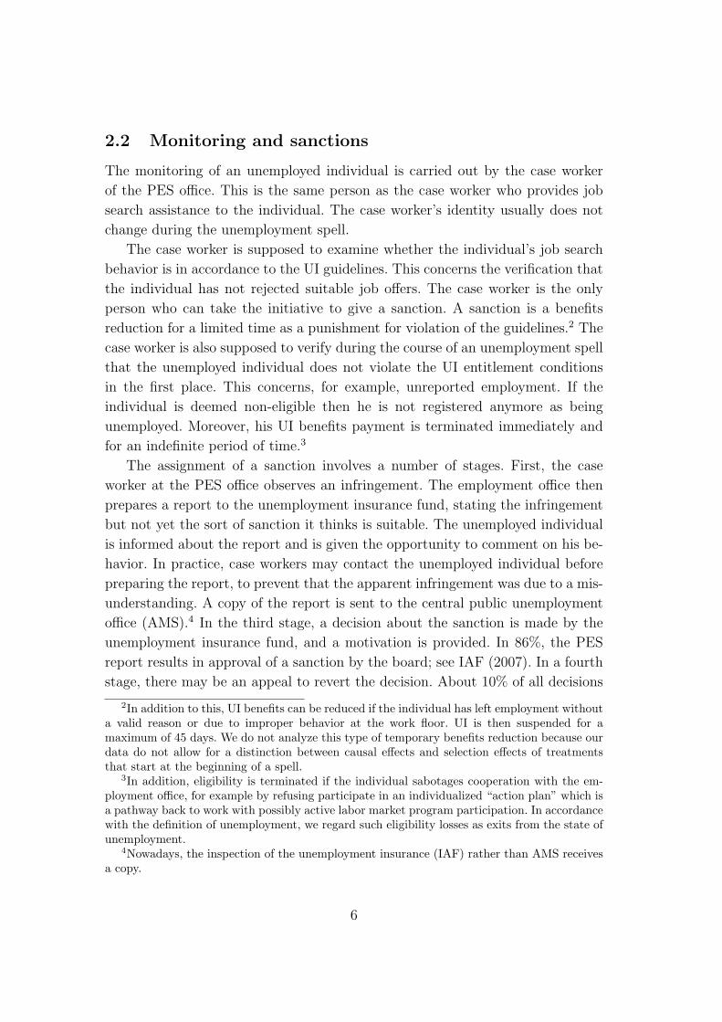
2.2 Monitoring and sanctions

The monitoring of an unemployed individual is carried out by the case worker

of the PES office. This is the same person as the case worker who provides job

search assistance to the individual. The case worker’s identity usually does not

change during the unemployment spell.

The case worker is supposed to examine whether the individual’s job search

behavior is in accordance to the UI guidelines. This concerns the verification that

the individual has not rejected suitable job offers. The case worker is the only

person who can take the initiative to give a sanction. A sanction is a benefits

reduction for a limited time as a punishment for violation of the guidelines.2 The

case worker is also supposed to verify during the course of an unemployment spell

that the unemployed individual does not violate the UI entitlement conditions

in the first place. This concerns, for example, unreported employment. If the

individual is deemed non-eligible then he is not registered anymore as being

unemployed. Moreover, his UI benefits payment is terminated immediately and

for an indefinite period of time.3

The assignment of a sanction involves a number of stages. First, the case

worker at the PES office observes an infringement. The employment office then

prepares a report to the unemployment insurance fund, stating the infringement

but not yet the sort of sanction it thinks is suitable. The unemployed individual

is informed about the report and is given the opportunity to comment on his be-

havior. In practice, case workers may contact the unemployed individual before

preparing the report, to prevent that the apparent infringement was due to a mis-

understanding. A copy of the report is sent to the central public unemployment

office (AMS).4 In the third stage, a decision about the sanction is made by the

unemployment insurance fund, and a motivation is provided. In 86%, the PES

report results in approval of a sanction by the board; see IAF (2007). In a fourth

stage, there may be an appeal to revert the decision. About 10% of all decisions

2In addition to this, UI benefits can be reduced if the individual has left employment withouta valid reason or due to improper behavior at the work floor. UI is then suspended for amaximum of 45 days. We do not analyze this type of temporary benefits reduction because ourdata do not allow for a distinction between causal effects and selection effects of treatmentsthat start at the beginning of a spell.

3In addition, eligibility is terminated if the individual sabotages cooperation with the em-ployment office, for example by refusing participate in an individualized “action plan” which isa pathway back to work with possibly active labor market program participation. In accordancewith the definition of unemployment, we regard such eligibility losses as exits from the state ofunemployment.

4Nowadays, the inspection of the unemployment insurance (IAF) rather than AMS receivesa copy.

6

are asked to be reverted, but in only about 20% of these is the decision partly

or fully reversed. Subsequently, one may appeal against a sanction at the county

administrative court (Lansratten).

There are several unpredictable events in this process. The case workers do

not always observe that an unemployed has turned down a job offer. Whether

a report is written or not depends on the attitude of the case worker (Swedish

overviews, like IAF, 2006, state that case workers report themselves that there are

differences in interpretation of the regulations between counties and employment

offices and between individual case workers working at the same employment

office). The benefit sanction decision may also depend on the board members

attending the UI fund meeting. All this makes it unlikely that UI claimants

anticipate the imposition of the sanction with great accuracy.

Before the reform of February 5, 2001, the only available sanction was a 100%

reduction of the benefits level for a period of 10 to 60 days. The choice of the

length of the sanction period was supposed to take the (subjectively assessed)

expected remaining duration of unemployment into account. In practice, however,

only a period of 60 days was used.

As noted in Section 1, the Swedish monitoring system was (and is) notably

different from the systems in many other countries (see Grubb, 2000, for details

about the systems in other countries). First, monitoring and job search assistance

are carried out by the same case worker. In other countries, monitoring is typically

carried out by agencies that are distinct from the agencies providing job search

assistance. Secondly, after inflow into UI, monitoring mainly restricts attention to

job offer rejections. Other countries focus primarily on search effort, as captured

by the number of applications sent out or indicators of the willingness to adhere

to job search guidelines.

Accordingly, Sweden is an outlier in aggregate statistics of sanctions. First, the

number of sanctions issued is very low. Figure 1 displays this number per month,

between January 1999 and November 2004. In 2000, about 3000 sanctions were

issued, on an average stock of 210,000 full-time unemployed UI recipients. In Gray

(2003)’s ranking of countries by sanction occurrence (which, roughly speaking, is

defined as number of sanctions divided by the number of unemployed), Sweden is

the lowest among the nine European countries considered (Sweden 0.79, Germany

1.14, Belgium 4.2, Denmark 4.3, Finland 10.2, United Kingdom 10.3, Norway

10.8, Czech Republic 14.7, Switzerland 40.3). Figures in other OECD countries

are typically much higher than the Swedish figure as well. Abbring, Van den Berg

and Van Ours (2005) report that around 3% of the inflow of UI recipients receive

a sanction during the UI spell, in The Netherlands in 1993. Contrary to Sweden,

7

a number of these countries, including Germany, The Netherlands, and Denmark,

has witnessed strong increases in the occurrence of sanctions since the early 2000s

(see e.g. Svarer, 2007, and Schneider, 2008). We shall argue below that the low

Swedish sanction occurrence can be explained by institutional differences in the

monitoring system.

2.3 Policy change of the monitoring regime

The uniquely low occurrence of sanctions in Sweden can be explained by a low

effective level of monitoring. In the late 1990s it was felt that the magnitude

of the punishment (100% UI benefits reductions for 60 days) was too large in

the eyes of the case workers. After all, the case worker is primarily trying to

help the unemployed individual, and the former would find it morally difficult

to punish the latter harshly. This could prevent case workers from reporting

violations. At the time, many other countries have policies where sanctions are

smaller than 100% of the UI level. Accordingly, the Swedish government changed

the policy design on February 5, 2001 (see e.g. Government of Sweden, 2000, for

a substantiation of the above-given description of the motivation for the policy

reform). From that day onwards, UI is reduced by 25% for 40 days for first-

time offenders, and by 50% for 40 days second-time offenders. A third violation

during the same UI entitlement period entails a full loss of benefits until new

employment has been found. The decision to change the monitoring policy was

made on December 21, 2000, which is 1.5 month before enforcement. The public

employment office AMS arranged regional meetings to inform the case workers

about the policy change. These were held between the middle of February, 2001,

and April, 2001. Case workers complained that after these meetings certain details

of the new policy regime were still not clear to them (personal communications).

Despite the policy change, the occurrence of sanctions has remained very low

by international standards. In Subsection 4.3 we examine whether the occurrence

of sanctions in our individual data registers displays differences before and after

the implementation date.

8

3 Theoretical insights

3.1 A job search model with monitoring of job offer deci-

sions

In this subsection we present a job search model with monitoring of job offer

decisions. This model takes distinguishing features of the Swedish UI monitoring

system into account and has not been analyzed in the literature. It is a model

of optimal behavior of unemployed individuals given the presence of a particular

system in which sanctions can be imposed. The model helps to understand the

effects of such a system on individual behavior. It also provides insights into the

determinants of the rates at which jobs are found and sanctions are imposed and

the relationships between these rates.

Our point of departure is a basic job search model with a fixed individual

search intensity. Consider an unemployed individual who searches sequentially

for a job. Job offers arrive according to the rate λ. Jobs are heterogeneous in

their characteristics. For expositional convenience we take the wage as the only

possible job characteristic in this subsection. Offers are random drawings from a

wage offer distribution F (w). Every time an offer arrives the decision has to be

made whether to accept it or to reject it and search further. Once a job is accepted

it will be held forever at the same wage. During unemployment, a flow of benefits

b is received, possibly including a non-pecuniary utility of being unemployed. The

individual aims at maximization of the expected present value of income over an

infinite horizon.

It is well known that in this model, under some regularity conditions, the

optimal strategy of unemployed individuals can be characterized by a reservation

wage φ, giving the minimal acceptable wage offer. The transition rate to work

equals λ(1− F (φ)).

Now let us introduce monitoring in this model framework. We assume that

the case worker samples a fraction p of rejected job offers, and that on average

a fraction q of these rejected offers are deemed to be sufficiently suitable for the

unemployed worker. Then a fraction pq of the rejected offers should not have

been rejected. Accordingly, the sanction rate equals λF (φ)pq. If p = 1 then all

offers are monitored, and if p = q = 1 then each rejected offer entails a sanction.

For a given p and q, we assume that the individual does not know which rejected

offers are sampled or which are deemed acceptable by the case worker, but that

he does know the values of p and q.

Some individuals will be more willing to take the risk of being given a sanc-

9

tion than others, e.g. because they have a higher non-pecuniary utility of being

unemployed. Obviously, if p = q = 1 and the punishment is sufficiently severe in

comparison to a job with the lowest possible wage, then all job offers are always

accepted, and sanctions would never be given. To proceed, we need to be spe-

cific about what occurs after the imposition of a sanction. First of all, benefits

(b) are reduced substantially. Secondly, p is likely to increase. If the individual

again violates the rules concerning job offer decisions, and this is observed by the

case worker, then additional benefits reductions are imposed. We assume that the

punishment for additional violations is so severe that the individual will avoid

this at all cost, so we assume that all offers are accepted after imposition of a

sanction. This implies that sanctions are imposed at most once in a given spell

of unemployment. (A strategy in which individuals take a job upon imposition of

a sanction, and quit immediately in order to make a “fresh start” in UI, would

not be optimal: UI would be reduced again immediately after quitting because

of “insufficient effort to prevent job loss”; see Section 2.)

For simplicity, we assume that the parameters b1 (being the benefits level be-

fore a sanction is imposed), F, λ, p, q and the discount rate ρ are constant as a

function of unemployment duration. Upon imposition of a sanction, b is perma-

nently reduced from b1 to b2, with b2 constant as a function of unemployment

duration. As a consequence, both within the time interval before a sanction and

within the time interval after a sanction, the optimal strategy is constant over

time.

Let R1 and R2 denote the expected present value of income before and after

imposition of a sanction, respectively, and let φ1 denote the reservation wage

before the sanction. We obtain

ρR1 = b1 + λEF

[max{w

ρ, (1− pq)R1 + pqR2} −R1

](1)

ρR2 = b2 + λEF

[w

ρ−R2

](2)

with φ1 = (1− pq)ρR1 + pqρR2

Equation (1) can be understood by interpreting R1 as an asset for which the

return flow equals the flow of what one expects to gain from holding the asset.

The latter consists of two parts: (i) the flow of benefits, (ii) the job offer arrival

rate times the expected gain of finding an acceptable job over staying unemployed.

The second part is the mean over F of the gain corresponding to a wage offer w.

10

If one accepts w then the associated present value is w/ρ, so the gain is w/ρ−R1.

If one rejects it then there is a probability pq that one is caught, in which case the

associated present value is R2, and a probability 1 − pq that one is not caught,

with present value R1. The gain is again equal to the new present value minus

R1. The derivation of (2) is analogous. Equations (1) and (2) can also be derived

as Bellman equations from first principles.

Notice that with the strictest possible monitoring, i.e., p = q = 1, the outside

option when considering an offer is equal to a certain punishment, so then φ1 =

ρR2. This implies that extreme monitoring does not necessarily entail the absence

of punishments. With certain model parameter values, it may still be optimal for

an individual to prefer a sanction and a forced future job offer acceptance over

a current low offer. This is particularly likely if the offer under consideration is

much lower than the average offer, and if the punishment b2 − b1 is small.

It is also interesting to consider the expected present value R1 and optimal

reservation wage φ1 in the absence of a monitoring system,

ρR1 = b1 + λ

∫ ∞

φ1

(w

ρ− R1)dF (w), with ρR1 = φ1 (3)

By elaborating on equations (1) and (2) we obtain the following expression

for φ1,

φ1 = pqb2+(1−pq)b1+λ

ρ

[(1− pq)

∫ ∞

φ

(w − φ1)dF (w) + pq

∫ ∞

0

(w − φ1)dF (w)

]

which has a similar structure as the reservation wage equation in a standard job

search model. Clearly, the latter is obtained by imposing p = q = 0. For general

p, q, we obtain a weighted average of the reservation wage in a market without

monitoring, and the present value flow after having been punished.

Using obvious notation, the transition rates from unemployment to employ-

ment before and after imposition of a sanction equal

θu,1 = λ(1− F (φ1)) and θu,2 = λ (4)

For a system with given p and q, the probability that a sanction occurs before

a job exit is equal to λpqF (φ1)/(λpqF (φ1) + λ(1− F (φ1))) = pqF (φ1)/(1− (1−pq)F (φ1)). This can be seen by noting that a newly unemployed individual faces

competing risks (a sanction and job exit) with constant rates λpqF (φ1) and θu,1,

respectively. The proportionate effect of the sanction on the job exit rate equals

11

θu,2/θu,1 = 1/(1−F (φ1)). This correspond to a parameter of the empirical model.

The additive effect of a sanction on the mean accepted wage equals EF (w) −EF (w|w > φ1). The empirical model contains a parameter that captures the

additive effect on the mean log accepted wage EF (log w)−EF (log w|w > φ1). Of

course the empirical parameters are not constrained to have a particular sign,

and they may themselves depend on deeper determinants and characteristics of

the individual and the labor market.

The additive effect on the job exit rate equals θu,2 − θu,1 = λF (φ1). Notice

that this is bounded from above by λ.

3.2 Theoretical predictions

A number of insights follow from the model. Consider the general case where the

model parameters are such that φ1 > w: the reservation wage before a sanction is

imposed exceeds the lowest possible wage offer in the market. This is a necessary

condition to observe sanctions at all. It is clear that R1 > R1 > R2, and conse-

quently φ1 > φ1. From the point of view of the individual, monitoring reduces

the expected present value, and so does an actual punishment in a world with

monitoring. By implication, θu,1 < θu,2, and both are larger than the transition

rate in a world without monitoring.

Consequently, monitoring affects the transition rate of all individuals (except

for those who have a very low reservation wage φ1 anyway). This is the ex ante

effect of the monitoring system, as opposed to the ex post effect due to imposition

of a sanction.

Notice that if φ1 ≤ w then the individual probability of job acceptance is

equal to one, so there will not be any sanctions. If the case worker is very lenient

(q = 0) then the sanction rate is zero as well. Conversely, we have seen that in the

strictest possible monitoring system (p = q = 1), an individual may still prefer

to reject a low-wage offer in favor of a sanction. This reflects a first fundamental

difference with monitoring schemes that target an endogenously chosen level of

search effort by the individual (see Abbring, Van den Berg and Van Ours, 2005, for

a theoretical analysis). In the latter scheme, perfect monitoring leads to absence of

sanctions, even if the punitive benefits reduction is small. This is because perfect

search effort monitoring is instantaneous and continuous in time and the effort

constraint will be strictly enforced after a violation. Perfect monitoring of offers

only takes place after offer rejections, and a rejection followed by a sanction may

be worthwhile if it is followed by a high wage offer at a later point in time.

It is interesting to consider the ex post effect and the occurrence of sanctions

12

for different subgroups of individuals. First, consider individuals for whom F (φ)

is very small. Since φ1 := (1 − pq)ρR1 + pqρR2, it follows that their expected

present value of unemployment after rejection of an offer is low. At the same

time, they are unlikely to reject an offer and therefore unlikely to get a sanction.

These may be individuals with a low R1 due to a low job offer arrival rate λ and

low benefits b1. Their sanction effect is small as well. Notice that for moderate

values of F (φ1), the probability pqF (φ1)/(1 − (1 − pq)F (φ1)) that a sanction

occurs before a job exit can still be extremely small if q is very small. In that

case the sanction effect is not necessarily extremely small.

Secondly, consider the opposite case where F (φ) is large (i.e., close to one).

This may capture long-term unemployed individuals who enjoy generous benefits

b1 whereas their skills have become obsolete and most offers that are made to

them concern low-skill jobs with wages below b1 (see Ljungqvist and Sargent,

1997, for an equilibrium analysis). Such individuals have a very high sanction

rate and sanction effect. But now let us consider what happens if individuals

can optimally choose their search effort s as well. Let the job offer arrival rate

now be specified as λs, and let the search cost flow c(s) be a convex increasing

function of s with c(0) = c′(0) = 0, so that the instantaneous income flow before

a sanction equals b1− c(s). The optimal value of s before a sanction follows from

maximization of the right-hand side of the suitably adjusted equation (1), leading

to

c′(s) = max{0, λ

ρ

∫ ∞

φ

(w − φ1)dF (w)− λpq(R1 −R2)}

If φ1 is at the upper bound of the support of F , then the integral in the above

expression vanishes, implying that s = 0. The same result holds for values of

φ1 close to the upper bound. If the monitoring regime is stringent then the last

term on the right-hand side increases, so the reduction of optimal search effort

is exacerbated. In sum, when these individuals can choose their level of search

effort, then offer decision monitoring will be counteracted by a reduction of search

effort. To put it bluntly, monitoring of offer decisions causes individuals with high

benefits (or a high utility flow of being unemployed) to prevent that they will ever

get an offer. The ex ante effect of monitoring is then perverse: more monitoring

implies a lower job exit rate. We view this as a potentially important insight.

Whereas job search effort monitoring always generates a positive ex ante effect,

job offer decision monitoring does not.

We briefly mention two other differences between job search effort monitoring

13

and job offer decision monitoring. These concern outcomes after the sanction.

Recall that we assume perfect monitoring after the sanction. The first of the

two differences concerns the magnitude of the ex post effect on the job exit rate.

Suppose that search effort s is endogenously determined. In the case of job offer

decision monitoring, the job exit rate after a sanction equals θu,2 = λs2, where s2

is the optimal search effort after a sanction. Conversely, in the case of search effort

monitoring, this rate equals λs∗(1− F (φ2)), where φ2 is the optimal reservation

wage after a sanction and s∗ is the minimum required search effort as postulated

by the UI agency. In the latter case, by choosing an appropriately high s∗, the job

exit rate, and by implication the ex post sanction effect, can be pushed upwards

to arbitrarily high values. In the former case this is not possible. Intuitively, the

effect of job offer monitoring is bounded from above by the rate at which job offers

arrive. (Of course, by pushing up s∗∗ in search effort monitoring, the privately

incurred search costs c(s) increase at an even higher speed. Also, if s∗ becomes

very large then the distribution of the associated wage offers may change at the

margin.)

The fourth and final difference between the monitoring regimes was already

mentioned in the introduction of the paper, namely that the adverse effects of

sanctions on post-unemployment outcomes may be smaller with search effort

monitoring than with job offer decision monitoring. Perfect monitoring after a

sanction implies full compliance after the sanction. With job offer decision mon-

itoring, this means that compared to the situation before a sanction, punished

individuals now also have to accept all offers of jobs with the lowest wages. With

search effort monitoring, however, full compliance means that punished individu-

als have to search harder for any possible job. The latter includes both high-wage

jobs and low-wage jobs.

All results in this section generalize to non-wage job characteristics. Basically,

if the individual’s utility flow function depends on the wage and on other char-

acteristics then the role of the income flow variables in the present section is

replaced by the corresponding utility flows.

We finish this section by briefly mentioning some implications of the above

that are of importance for the specification of the empirical model. The empir-

ical model is a reduced-form model in which hazard rates are allowed to vary

over time and across observed and unobserved individual characteristics. The

implications below also follow from models with monitoring of an endogenously

determined search effort (see Abbring, Van den Berg and Van Ours, 2005). First,

at the individual level, the transition rate from unemployment to employment

makes a discrete upward jump upon imposition of a sanction. If individuals are

14

homogeneous then the size of this jump, which is the causal effect of the sanction

treatment, can be estimated from an unemployment duration model in which the

moment at which a sanction occurs is a time-varying exogenous covariate.

Empirical analyses of duration data from a market with a given monitoring

system do not allow for non-parametric identification of ex ante effects. So such

analyses cannot be used to evaluate the effect of the monitoring system on unem-

ployment durations. The latter objective requires at least some observed variation

in the monitoring system itself.

Both the transition rate from unemployment to employment and the rate

at which a sanction arrives depend on all the variables that the individual uses

to determine his strategy. This is because both depend on φ1 (provided that

φ1 > w). In reality, individuals are heterogeneous with respect to determinants

of search behavior. Suppose that the individuals know their own value of some

characteristic but that these values are not observed in the data. As we argued

in Section 1, with punitive treatments, such a setting is plausible. Then both

the transition rate from unemployment to employment and the rate at which

a sanction is imposed depend on this unobserved characteristic. This creates

a spurious relation between the duration until a sanction is imposed and the

duration of unemployment. Note that a similar spurious relation is created if the

policy parameters p and q of the sanction rate itself differ across individuals in a

way that is not observed by the researcher.

4 Data

4.1 Data registers

Our main data are taken from a combination of two Swedish register data sets

called Handel (from the official employment offices) and ASTAT (from the un-

employment insurance fund). Handel covers all registered unemployed persons.5

It contains day-by-day information on the unemployment status, whether the

unemployed is covered by UI, entries into and exits from active labor market pro-

grams and part-time unemployment, and the reason for the unemployment spell

to end. As a rule, UI spells end in transitions into re-employment, education,

social assistance, or other insurance schemes. Handel also includes a number of

background characteristics, recorded at the beginning of the unemployment spell.

ASTAT provides information on all benefits sanctions, including information on

5According to Carling, Holmlund and Vejsiu (2001), more than 90% of the individuals whoare ILO-unemployed according to labor force surveys also register at the employment offices.

15

the timing of the sanction, the main reason for the sanction, and the size of the

benefit reduction.

Our observation window runs from January 1, 1999 until December 31, 2003.

We only use information on individuals who become unemployed at least once

within the observation window. An individual becomes unemployed at the first

date at which he registers at the employment office as being ”openly” unem-

ployed. We ignore unemployment spells that are already in progress at the be-

ginning of the observation window, because using them would force us to make

assumptions about the period before the beginning of the window. We focus

on re-employment durations, and consider any employment, full-time or part-

time, which is retained for at least 10 days as employment. At later stages we

separately model the decision to accept part-time employment. UI spells that ter-

minate for other reasons than re-employment are considered being right-censored

re-employment durations. We stop time while unemployed are enrolled into active

labor market programs. Robustness analysis shows that our results are insensitive

to this restriction. Apart from that, individuals are only followed up to December

2004. Ongoing spells at that date are right-censored. We restrict our analysis to

everyone who was between 25-55 at the time of entry into unemployment and

covered by UI.6 We only model the first sanction during an unemployment spell.

Any effects of a second or third sanction are considered to be a part of the first

sanction treatment effect. Finally, we exclude all unemployment spells for a spe-

cific individual that occur after a spell during which a sanction was given to that

individual. This is because we exploit multiple spells to enhance the quality of

the results, and we cannot rule out that a sanction also affects future subsequent

spells.

The sanction and unemployment data are combined with survey data on wages

and hours worked from Statistics Sweden’s wage statistics. It provides us with

information on actual wages per time unit, so these are not wages created from

annual earnings and some measurement of hours worked. The wage is recorded as

the monthly full-time equivalent wage. The survey is collected annually (during

the fall) by Statistics Sweden in cooperation with employer organizations. It

covers the whole public sector, all large private firms and a random sample of

small firms (about 50 percent of all private sector employees). If we observe a

wage within one year after the exit to employment we use this wage, otherwise

the wage is considered to be missing. The information on hours worked is used

6We also exclude disabled individuals and everyone who some time during the researchperiod participated in sheltered employment, because these are intended for unemployed withsome kind of disability or handicap.

16

to construct an indicator variable for full-time employment, defined as working

34 hours or more a week.

The wage data also include individual occupations. These are classified us-

ing SSYK 96 (Standard for svensk yrkesklassificering 1996 ), which follows the

international standard ISCO-88. Each occupation is classified into 355 separate

groups of occupations (four digits). The first digit classifies occupations by the

general qualifications required to perform the tasks associated with each occu-

pation. It divides the occupations into four levels: the occupations in group 1

normally require no or limited education, level 2 occupations require high school

competence, level 3 occupations short university education, and the occupations

at level 4 require longer university education (3-4 years or more). Additional digits

capture the specialization skills associated with each occupation. We matched oc-

cupations to individual education levels taken from Statistics Sweden’s database

“Louise”.

4.2 Descriptive statistics

Table 1 provides statistics on the unemployment spells and the duration until a

sanction. In Subsection 5.4 below we explain that we choose to estimate models

with an endogenously stratified sample. The current subsection provides infor-

mation on the full data set and on the sample used for the model estimation.

A large part, 65.7%, of the re-employment spells in our analysis data set is not

right-censored. Remember that the remaining 34.3% of the spells are ongoing at

the end of the data period, or UI spells that are completed for other reasons

than re-employment. During only 0.18% of the unemployment spells in our full

sample a sanction is imposed, compared with 8.4% in the data set used for the

model estimation. Relatively many sanctions, 46.7%, are imposed during the first

100 days of unemployment. There is also a substantial number of sanctions, 16%,

imposed after 300 days or more in unemployment. Because of censoring, these

raw figures underestimate the incidence of sanctions and the duration at which

these are imposed. About 8% of the sanctions are given to second-time offenders

and only about 0.5% to third-time offenders.

Table 2 provides statistics on the job-quality measures. For about 35% of the

spells for which observe an exit to employment we observe the wage within one

year after the exit. Not observing the wage can be due to fact that the individual

is employed in small private firms or due to fact that the individual already

left employment before the time of the survey. As the wage survey is conducted

annually, the mean time from the exit to employment to the time of the wage

17

survey is about half a year (179 days). Note that, because the survey is mainly

conducted during the fall and because there is seasonal variation in exits from

unemployment, the time from the exit to the survey is not uniformly distributed

over 1-12 months. The mean monthly wage is about SEK 17,840 among the

individuals for whom we observe the wage, and about 57% of these individuals

have full-time employment. Furthermore, 57% find a job in the public sector, 31%

in a large private firm, and 21% find a job in a small private firm. Here, a large

firm is defined as having 200 employees or more.

The missing wage data may not be missing at random. First of all, remember

that we observe the wage for all public sector employees, all employees at large

private firms, and a random sample of those working in small firms. Suppose that

individuals who are sanctioned accept lower wages on average. Small firms tend

to pay lower wages than large firms, so there may be a selectivity in the wage

observations, and this may lead to an under-estimation in absolute values of the

negative effect of sanctions on wages. To explore this, we specify a logit model

for the choice between accepting public sector or private sector employment, and,

given the choice to enter the private sector, a logit model for the choice between

accepting employment in a large firm or a small. In both models we control for

a number of covariates, such as sex, age, level of education, time of inflow into

unemployment, regional variables, level of education, the kind of profession the

unemployed is searching for and whether the unemployed has education respec-

tively previous experience in that occupation. We estimate these two logit models

jointly using maximum likelihood, and the results are presented in Table 3. The

results show no evidence of selection due to a sanction into small private firms.

We therefore feel confident in assuming that it is random whether we observe the

wage or not. The same holds for hours worked.

The second concern regards the fact that, in most cases, some time elapses

between the exit from unemployment and the wage survey. It means that we do

not observe the first wage after unemployment for individuals who have quickly

moved into a second or even third employment. We neither observe the wage for

those who have become unemployed or left the labor market entirely before the

wage survey is conducted. Both these factors may bias our job quality estimates. If

there is an effect of a sanction on the job security, relatively more individuals with

sanctions will go back into unemployment before the time of the wage survey. As

these individuals can be expected to be on the lower end of the wage distribution

it will also bias our job quality estimates upwards. In addition, if unemployed

with sanctions move relatively faster into a second employment, with a higher

wage, it will also bias our job quality estimates upwards. To proceed ahead, even

18

with these potential biases we find significant negative job quality effects.

4.3 Around the date of the monitoring policy regime change

In this subsection we provide descriptive statistics on the occurrence of sanctions

shortly before and after the policy change of February 5, 2001. Ideally, a change

in the monitoring regime offers an opportunity to investigate the ex ante threat

effect.

As apparent from Figure 1, the reform did not lead to a substantial increase

in the number of sanctions issued. Instead, apart from seasonal fluctuations, this

number has been increasing slowly and steadily after the reform.

In addition, there are large regional differences in the development of the

number of sanctions over time. Regional variation is to some extent due to the

fact that only the individual case worker and the chief of the local PES office

decide about whether a report should be sent to the unemployment insurance

fund (recall the statements in IAF, 2006 mentioned in Subsection 2.2). Table 13

lists the mean number of sanctions per quarter by region. In Figure 2 and Figure

3 we display an index of the quarterly number of sanctions for each of the years

2000-2004 using the quarters of 1999 as base period. An index value of 2 in 2003

means that sanctions are twice as frequent in 2003 as in the same quarter in

1999. We display this for three regions in the southern and the central parts of

Sweden, respectively. They reveal a wide regional variation in patterns after 2000.

We observe permanently increased sanction numbers in some regions, no change

in some other regions, and temporary increases in sanctions in yet other regions.

To focus more closely on the moment of the policy change, we list in Table 13

the ratio between sanction occurrences in the first quarter of 2001 and the first

quarter of 2000, and the same for the other quarters in 2001 and 2000. These

ratios are purged from seasonal variation. The statistics confirm the patterns in

Figure 2 and Figure 3.

Clearly, from a methodological point of view, it is hard to reconcile the erratic

and region-specific fluctuations in the occurrence of sanctions after the policy

change to the idea of exploiting the discontinuity in the monitoring system for

the estimation of ex ante effects. But at the very least we may conclude that the

occurrence of sanctions has not increased substantially after the policy change.

According to our theoretical model, there are two possible explanations for this.

First, the case workers have decided to not to act on policy change but instead

to continue not to recommend sanctions in case of violations, because they find a

25% benefits reduction still too severe. Obviously, in the new system, the punish-

19

ments are less harsh than before, but from an international perspective they are

still substantial. In the Netherlands, where sanctions are less severe, and monitor-

ing is carried out by different individuals than the case workers, the individuals

who carry out the monitoring state that they are less likely to issue a sanction if

they feel that the unemployed individual faces adverse labor market conditions

(see Van den Berg and Van der Klaauw, 2006). In agreement to this, studies

with Dutch data find that individual characteristics that are associated with a

low exit rate to work are also associated with a low sanction rate, confirming

that the monitoring intensity depends positively on the individual’s labor market

conditions. In terms of our theoretical model, this first explanation would mean

that the policy change does not lead to any changes in the parameters in the

decision problem for the unemployed individual.

The second explanation for the low occurrence of sanctions after the policy

change is that a more stringent monitoring scheme may motivate many individu-

als to avoid violations at all costs, i.e. that the policy change induced a strong ex

ante effect. The net effect of an increase in the monitoring and a decrease in vio-

lations may then be that the occurrence of sanctions remains low. In terms of our

theoretical model, the policy change is captured by an increase of q which leads

to a decrease of φ1 such that virtually all offers are accepted. In Subsection 3.2 we

also showed that an increase of q may lead to a reduction of search effort to zero,

such that no offers are generated in the first place, and consequently sanctions do

not occur. However, this is potentially only relevant for a subset of individuals

whose benefits are high compared to the wages they may earn. Obviously, a zero

effort gives rise to extremely long unemployment spells. (A third explanation is

that monitoring was virtually perfect in both regimes, but this seems borne out

by the motivation for the policy change as well as by the variation in enforcement

across case workers.)

To distinguish between these explanations we have to examine the unem-

ployment duration outcomes and the post-unemployment outcomes. The first

explanation implies that the job exit rate θu,1 is the same in both regimes. The

second explanation implies that this rate changes after the policy change. This

is because in the first case φ1 does not change whereas in the second case it de-

creases. The identification of a subgroup of individuals with zero search effort in

the new regime seems to be beyond what is empirically feasible, but we should

keep in mind that such a subgroup may exist. We return to the issues of this

subsection after having presented the duration model estimates in Section 6.

20

5 Empirical model

5.1 Timing of Events model

This section presents our empirical model. In Subsection 5.1, we present a basic

bivariate duration model, for the duration until employment and the duration

until the imposition of a sanction. This “timing of events” approach (Abbring

and Van den Berg, 2003) is the standard approach in the literature on sanction

effects. In Subsection 5.2 we extend this well known model into our full model,

incorporating the job quality into the same model.

We normalize the point of time at which the individual enters unemployment

to zero. We are interested in investigating how the duration ts until the imposition

of a sanction affect the duration until employment, te. In order to illustrate the

basic identification problem, suppose that we observe that the individuals who

are sanctioned at ts have relatively short unemployment durations then this can

be for two reasons: (1) the individual causal sanction effect is positive, or (2) these

individuals have relatively favorable unobserved characteristics and would have

found a job relatively fast anyway. The second relation is a spurious selection

effect. To control for such spurious effects, we analyze both the distribution of

te for a given ts and the distribution of ts jointly. It is well known that these

distributions can be conveniently represented by the corresponding hazard rates.

First, consider individuals who are unemployed for t units of time. We assume

that all individual differences in the re-employment rate at t can be characterized

by observed characteristics x, unobserved characteristics Ve, and a sanction effect

if a sanction has been imposed before t. Next, consider the rate at which a sanc-

tion is imposed on an unemployed individual. Similarly as for the re-employment

hazard, we assume that all individual differences in this rate can be character-

ized by observed characteristics x and unobserved characteristics Vs. We further

assume that the re-employment rate denoted by θe(t|x, Ve, ts), and the sanction

rate denoted by θs(t|x, Vs) both have the familiar Mixed Proportional Hazard

(MPH) specification, this gives

θe(t|x, Ve, ts) = λe(t) exp(x′βe) exp(I(t > ts)δ(t|ts, x)) Ve, (5)

θs(t|x, Vs) = λs(t) exp(x′βs) Vs. (6)

Here I(.) is an indicator function taking the value one if the argument is true

and zero otherwise. δ(t|ts, x) then represent the sanction effect, which we allow to

vary both with observed characteristics and with time, t−ts, since the imposition

21

of a sanction. Further, λe(t) and λs(t) represents the duration dependence in the

re-employment hazard and the sanction hazard, respectively.

Equations (5) and (6) give the joint distribution of te, ts|x, Ve, Vs. Our data

provide information on the distribution of te, ts|x. Let G denote the joint distribu-

tion of Ve, Vs|x in the inflow into unemployment. It is clear that a specification of

G, together with the specification of the joint distribution of te, ts|x, Ve, Vs, fully

determines the distribution of te, ts|x, and thus the data. Abbring and Van den

Berg (2003) show that all components of this model, including δ, are identified,

provided we make assumptions similar to those usually made in standard uni-

variate MPH models with exogenous regressors. Identification is semi-parametric

in the sense that given the MPH structure, it does not require any parametric

assumptions on the components of the model. It allows for general dependence

between te and ts through both the causal effect of sanctions and related unob-

servables.

The identification does not require conditional independence assumptions or

exclusion restrictions on the effects of x on the individual hazard rates θe and θs.

This is important, since all variables that affect the sanction rate plausibly also

affect the re-employment rate, and vice versa. Instead, identification is based on

the timing of events, i.e. the timing of sanctions and of exits out of unemployment.

Intuitively, what drives the identification of the sanction effect, δ, is the extent to

which the moments of a sanction and the moment of exit to employment are close

in time. If a sanction is quickly followed by exit to employment, no matter how

long the elapsed unemployment duration before the sanction, then this is evidence

of a causal effect of a sanction. Any spurious selection effects through dependence

between Vs and Ve, gives a second relation between the two duration variables,

but it can be shown that that relation does not give rise to the same type of

quick succession of events. So the interaction between the moment of exit and

the moment of a sanction in the conditional rate of events allows one to distinguish

between the causal effect and selectivity. The Monte Carlo simulations in Gaure,

Røed and Zhang (2007) support the use of this approach by showing that the

estimates of the parameters of interest are robust with respect to functional form

assumptions.

Formally, identification of the model relies on a number of implicit and ex-

plicit assumptions. We assume that a sanction does not affect the re-employment

rate before the moment of the sanction, whereas the effects of the unobserved

covariates are fixed during the spell. The former is often referred to as the no-

anticipation assumption. With sanctions, the moment at which an individual is

caught is almost by definition unanticipated by the individual. As explained in

22

Section 2 there are also several sources of unpredictability in the sanction process,

which makes it even less likely that UI claimants anticipate the actual timing of

the sanction. Next, since we specified the hazard rate it means that we implicitly

assumed that there is a random component in the assignments that is indepen-

dent of all other variables. Based on the randomness in the sanction process

and the obvious randomness in the job-search process, we are confident that this

assumption is satisfied.

Identification with single-spell data also requires that (i) x on the one hand

and Vu, Vs on the other hand are independent in the inflow, and (ii) there is

sufficient variation in x. However, since we often observe multiple UI spells for a

given individual we can relax these two assumptions. We assume that multiple

spells for one individual given the characteristics are statistically independent of

each other, that the unobservables Vu and Vs are fixed across spells, and that

the length of intervening spells between any two unemployment spells of a single

individual are independent of Vu and Vs. As shown by Abbring and Van den Berg

(2003), under these assumptions, the assumptions (i) and (ii) can be discarded.

5.2 Extension to post-unemployment outcomes

We measure job quality by the monthly wage, and by whether the accepted job is

full-time or part-time. These outcomes can be expected to depend on unobserved

factors that are related to the unobserved determinants of the job exit rate and

the sanction hazard. For instance, ability plays an important role for all these

outcomes. In order to identify the effects of a sanction on the job quality we need

to impose some structure. We assume that the causal effect and the selection

effect only affect the mean log wage, and we assume that these effects are additive.

Specifically, the wage at the start of the new employment can be expressed as

ln w = x′βw + γwI(ts < te) + Vw + ew, (7)

where γw is the sanction effect, Vw unobserved individual characteristics, and ew

is an error term which reflects random variation in the hourly wage. ew is assumed

to be normally distributed with mean zero and variance σ2w. Similarly, we specify

the decision to accept full-time employment as

h = 1[x′βh + γhI(ts < te) + Vh + eh > 0] (8)

23

where h = 1 if the individual finds full-time employment. As before γh is the

sanction effect, Vh unobserved individual characteristics, and eh an error term

which reflects truly random variation. eh is assumed to have a standard logistic

distribution.

We also acknowledge the tight link between the unobserved effects in the two

job quality measures and the unobserved effects in the sanction hazard and the

exit hazard. We take a simple linear form for this relation, as

Vw = βweVe + βwsVs, (9)

and

Vu = βheVe + βhsVs. (10)

Here βwe,βws, βhe, and βhs captures the correlation between the unobservables in

the model.

Abstracting from censoring, the joint density of Te, Ts,W,H|x at Te = te, Ts =

ts, W = w,H = 1 is then

∫ ∞

0

∫ ∞

0

(λe(te) exp(x′βe)ve exp(I(te > ts)δ(te|ts, x))

exp

(−exp(x′βe)ve

[ ∫ min(te,ts)

0

λe(k)dk+I(te > ts)

∫ te

ts

λe(k)δ(k|ts, x)dk

])

λs(ts) exp(x′βs)vs exp

(− exp(x′βs)vs

∫ ts

0

λs(k)dk

)×

1

σ√

2πexp

(− (ln w − x′βw − γwI(te > ts)− βweve − βwsvs)

2

2σ2

)×

exp(x′βh + γhI(te > ts) + βheve + βhsvs)

1 + exp(x′βh + γhI(te > ts) + βheve + βhsvs)G(ve, vs) (11)

We jointly estimate this full model.

Consider identification of this full model. In short the duration part of the

model identifies G, and given this we can estimate βwe,βws, βhe, and βhs. We have

then uncovered the selection process in the job quality decisions. It allows us to

integrate out the unobserved effects in the wage equation and the hours worked

equation.

24

5.3 Parameterizations

Given the assumptions discussed above, including the MPH structure, the model

is identified without any further parametric restrictions. However from a com-

putational point of view we need to specify some parametric structure. We take

flexible specifications of both the duration dependence functions and the bivari-

ate unobserved heterogeneity distribution. We take both λe(t) and λs(t) to have

a series representation

λi(t) =∑

j=0,1,...

αijtj. (12)

Note that with a large number of polynomials any duration dependence pattern

can be approximated closely. In the basic analysis we take polynomials of seventh

order and lower for the exit hazard, and polynomials of third order and lower for

the exit hazard. We have experimented with both more and less polynomials.

The results are insensitive such changes, unless the number of polynomials are

very few.

We use a bivariate discrete distribution with unrestricted mass point locations

for G. This provides a very flexible specification as well as being computationally

feasible. In our basic specification we take Ve and Vs to have two points of sup-

port each: V 1, V 2 and V 3 and V 4, respectively. The associated probabilities are

denoted as follows:

Pr(Ve = V 1, Vs = V 3) = p1, Pr(Ve = V 2, Vs = V 3) = p2

Pr(Ve = V 2, Vs = V 3) = p3 and Pr(Ve = V 2, Vs = V 3) = p4,(13)

with 0 ≤ pi ≤ 1 for i = 1, .., 4, and p4 = 1− p1 − p2 − p3.

5.4 Weighted exogenous sampling maximum likelihood

estimation

Our full data set contains over 1.6 million unemployment spells of about 827,000

individuals. In only about 3000 of these spells a sanction is imposed. To keep

the empirical analysis manageable from a computational point of view and at

the same time have enough spell with sanctions, we use weighted exogenous sam-

pling maximum likelihood (WESML) estimation with an endogenously stratified

sample. This method has not been used yet in the context of bivariate dependent-

duration models, and is not widely used in labor economics in general (see Ridder

and Moffitt, 2007, for a detailed econometric overview).

25

With exogenous sampling, a sequence of individuals is sampled and their out-

comes and characteristics are recorded. In contrast, with endogenous sampling, a

sequence of outcomes are sampled and the characteristics of the individuals with

these outcomes are recorded. Endogenous stratified sampling has, for instance,

been used in transportation economics (see e.g. Manski and Lerman, 1979, and

Garrow and Koppelman, 2004) and in biostatistics. A key example is the study

of rare diseases, for which it is reasonable to over-sample individuals with rare

disease.

In our case we wish to use all information on the individuals who receive a

sanction. We therefore sample all individuals who experience at least one sanc-

tion in the observation window, and take a smaller random sample (14,000) of

individuals who do not experience a sanction during this window. For these in-

dividuals, both sanctioned and non-sanctioned, we take all unemployment spells

during the research period, leaving us with about 35,000 spells.

As shown by Manski and Lerman (1977), WESML provides a consistent es-

timator. Each observation is weighted with the ratio between the population

fraction and the sample fraction of the strata it belongs to. Define Li as individ-

ual i’s contribution to the likelihood function. Then, formally, WESML amounts

to maximization of the weighted likelihood function

ln Lw =N∑

i=1

S∑s=1

d(s)Q(s)

H(s)Li (14)

where d(s) is an indicator variable taking the value one if individual i experience

outcome s, Q(s) the actual fraction of the population selecting alternative s, and

H(s) the probability that an individual selecting alternative s is included in the

sample. In our case, we have two alternatives: s = 1 if the individual experiences

a sanction during the research period, and s = 0 otherwise.

Inference on precision also has to be adjusted. Manski and Lerman (1977)

show that the appropriate covariance matrix is the familiar sandwich estimator

V = A−1BA−1, with

A = −E[(∂2 ln Li

∂θ∂θ′)θ=θ∗

]and B = E

[(∂ ln Li

∂θ)θ∗(

∂ ln Li

∂θ′)θ=θ∗

].

The WESML estimates are not efficient. Efficient estimators based on endoge-

nously stratified samples are developed in Imbens and Lancaster (1996). The basic

idea is to use the populations moments as moment restrictions in order to improve

26

efficiency. We decide not to pursue this approach. The reason for this is that our

analysis sample will be large, and efficiency is not a crucial issue. Furthermore,

in our case the most efficient estimator is to use the full sample of 1.6 million

unemployment spells and estimate using standard ML.

6 Results

6.1 Baseline results

This subsection presents the baseline estimation results for the Timing of Events

model, with a sanction effect that is constant over the population and over time.

In the next subsection, we investigate the importance of temporal and cross-

sectional variation in δ. From Subsection 6.3 and onwards we present the results

from our full model, testing whether a sanction affects the quality of the accepted

employment.

Table 4 presents the parameter estimates of the basic model. In this estimation

we use the analysis sample presented in Section 4, and estimate the model using

WESML. We use the individual characteristics listed in Table 2, and a set of

inflow time dummies as observed covariates. As we will not normalize the scale

of the unobservables, we have to exclude a constant from the regressors and one

category from each set of dummies.7 We further normalize the two constants in

the duration dependence, αs0 = αe0 = 1.

The parameter of interest is the sanction effect δ. The estimate of δ is positive

and significant at the 1% level. The estimate indicates that a sanction increases

the transition rate to employment with about 23%. Compared to other studies

on UI sanctions effects on the job exit rate this is a rather small effect. For the

Netherlands, Abbring, Van den Berg and Van Ours (2005) find that a sanction

doubles the job exit rate. For Switzerland, Lalive, Van Ours and Zweimuller

(2005) estimate that the job exit rate increases with about 25% if a sanction

warning is issued and with another 25% if a sanction is actually imposed. For

Denmark, Svarer (2007) estimates increases of about 50% for men and a doubling

for women. We can only speculate about the reasons behind these differences.

Presumably, the institutional settings play a role. As described in Section 3.2,

a system of job-offer decision monitoring, like the system in Sweden, places a

natural upper bound on the sanction effect, because even if all offers are accepted,

7Our base category consists of women, with neither education nor experience in their occu-pation, who do not need guidance, living in the central parts of Sweden, with less than highschool education and who started their unemployment spell in 1999.

27

the job exit rate is bounded from above by the job offer arrival rate. A system

where a minimum search effort is imposed after a sanction does not give rise to

such an upper bound. Moreover, after a sanction, unemployed workers in Sweden

may reduce their effort to zero in order to prevent further job offers and therefore

additional punishments.

The signs of the regressor effects on both hazards are mostly as expected.

Not surprisingly, we find selection on observables. For example, the dummy for

individuals with university education generates a negative selection effect: highly

educated unemployed have high re-employment rates and low sanction rates.

Omitting this dummy as an explanatory variable would have resulted in under-

estimation of δ (if it is not captured by the unobservables). Further as expected,

is the re-employment rate higher for highly educated, and for unemployed which

have education in their profession. The effect of the observables on the sanction

rate also reveals some interesting patterns. The gender dummy is insignificant,

indicating that discrimination is not important for the sanction decision. We also

note that the sanction effect is significantly lower among older workers.

Table 4 also reports the estimates for the baseline hazard as a set of coefficients

for the polynomials of order one to seven. In order to provide more intuition be-

hind these estimates we have produced two figures: Figure 4 and Figure 5, which

display the estimated duration dependence at daily basis for the exit rate and

sanction rate, respectively. Remember that the baseline hazard at time point zero

is normalized to one. The exit rates to employment initially decrease, but after

about 150 days of unemployment the exit rate starts to go down. For instance,

after 600 days in unemployment the re-employment rate is about 30% lower com-

pared with at the start of the unemployment period. Apparently, stigmatization

and discouragement play a significant role for individual unemployment dura-

tions. The sanction rate gradually rises with time spent in unemployment. After

about 300 days the maximum sanction rate is attained, and at longer durations

there is a tendency towards decreased sanction rate. This is consistent with the

fact that sanctions that are imposed because of some violation during the unem-

ployment spell cannot be given at the start of that spell.

6.2 Effect heterogeneity

We now allow the sanction effect to vary over the population. We first specify δ

as a function of explanatory variables x, as follows: δ = x′γ, for some parameter

vector γ that replaces the single effect parameter δ. Since our sample only con-

tains a limited number of sanctions, we only include a small number of variables.

28

We test for heterogeneous effects by sex, age, level of education, local unemploy-

ment rate, type of sanction regime and local sanction volume. Table 5 presents

the estimated sanction effects. The other estimates are very similar as for the

basic model, and are therefore not reported. We find interesting heterogeneous

treatment effects: the sanction effect is significantly lower for males, and signifi-

cantly lower for older unemployed. There is further no difference in the sanction

effect by level of education, nor by local unemployment rate. We also included

the regional occurrence of sanctions (number of sanctions divided by the number

of unemployed), interacted with the treatment. If stigma is an important part of

the sanction effect, the sanction effect should be lower in regions where sanctions

are more common. However, we find no such differences.

Next, consider how the monitoring regime affects the sanction effect. As ex-

plained in Section 2 the Swedish sanction regime was changed in February, 2001.

The reform introduced new, softer, sanctions, which reduced the size of the ben-

efit reduction from 100% to 25%. The new sanctions may influence the average

sanction effect in two ways. First, the new sanctions are softer so that we expect

the sanction effect to decrease for each individual. Second, the reform increased

the sanction volume, implying that unemployed who commits less serious viola-

tions are also sanctioned after the reform. These individuals are most likely more

sensitive to sanctions, which gives an upward tendency in the average sanction

effect. The effect of the reform on the average sanction effect is therefore theoret-

ically ambiguous. We find that the average sanction effect is significantly higher

under the new sanction regime. We draw two conclusions from this result: (i) un-

employed who commits less serious violations are more responsive to sanctions,

and (ii) the new softer sanctions are also considered as a severe punishment.

It is also possible that sanctions have an effect only shortly after they have

been imposed. To investigate this we introduce duration dependence in the effect

parameter, as follows: exp(δ) = exp(δ1+δ2(t−ts)). If δ2 is negative this means that

the sanction effect decreases over time. Table 6 reports the estimates of δ1 and

δ2. These results indicate very persistent effects of a sanction. We have multiplied

the coefficient for δ2 with 100. It means that the average sanction effect on the

re-employment hazard after 100 days is about 19%, compared to 20% directly

after the sanction has been imposed. There are several potential explanations

to this persistent effect. It is reasonable to believe that individuals who have

experienced a sanction are subject to intensified monitoring and attention from

the case workers. In addition, second time offenders are punished harder, so that

the persistent effect may be an effect of that the unemployed is eager to avoid

future sanctions.

29

6.3 Job quality

We now consider the effect of a sanction on characteristics of the subsequent

employment. From a welfare point of view, as well from the point of view of the

unemployed individual, any such effects are important. If the job accepted after

a sanction is similar to the job accepted in the counterfactual situation of no

sanction, then severe sanctions and intensive monitoring have less adverse effects

than otherwise.

Table 7 presents the estimates of the full model. The parameters of interest

are δw and δh, the sanction effect on the wage and hours worked, respectively. Our

estimates show a negative and significant (at 1% level) sanction effect on both the

wage and on hours worked. A sanction decreases the accepted wage with about

3.8%. We measure hours worked using an indicator variable taking the value

one for full-time employment and zero otherwise. Recalculated into marginal

effects the results in Table 7 imply that a sanction increases the probability to

accept part-time work with about 10.3 percentage points, or 15 percent. Part-time

work is more often associated with a less secure employment, and of course, a

lower income. We therefore interpret the effect on hours worked as a re-enforced

negative effect on the job quality. It means that a sanction has a quite large

negative impact on quality of the subsequent job.

The signs of the regressor effects on both the wage and hours worked are

as expected. Males receive higher wages compared to women. Unemployed with

high school education earn about 2% more than unemployed with less than high

school education. The corresponding number for unemployed with university edu-

cation is 11%. We find similar patterns for hours worked. Males, highly educated,

and unemployed in low employment areas, tend to find full-time employment

to a higher degree. This confirms that wage and full-time employment both are

perceived as attractive job characteristics.

6.4 Long run effects

It may be that the sanction effect on the accepted job is a short-term effect,

and that those who suffer a sanction catch up quickly, say after two or three

years. This would be in line with the results in Zijl, Van den Berg and Heyma

(2009), who find that temporary jobs often serve as a stepping-stone into regular

work. On the other hand it may also be the case that those who suffer a sanction

end up on a lower job quality trajectory, with long-term or even permanent job

quality effects. Obviously, if there are long run effect the negative welfare effects

of sanctions are smaller. Investigating the long run effects is thus crucial from a

30

policy perspective.

In order to investigate the long run effects of a sanction we re-estimate our

full model using the wage and full-time status after two, three and four years in-

stead of the wage and full-time status directly after the exit from unemployment.

We use the same full model as specified in Subsection 5.2, including a normally

distributed wage, a logit specification for the full-time part-time decision, and

a flexible specification of the observed and unobserved effects in the model. Ta-

ble 9 presents some descriptive statistics for these long run outcomes. Obviously,

we cannot observe the wage for those who have left the labor market and not

for those who once again are unemployed. As expected we therefore observe less

and less wages as time passes on after the exit to employment. It means that

we estimate these models with some reservations. However, as the wage several

years after the exit from unemployment is rarely observed, we find this exercise

meaningful.

Table 10 presents our long-term job quality estimation results. Here we only

present the sanction effects, but remember that the models also include the du-

ration until a sanction, as well as extensive controls for observed and unobserved

heterogeneity. We find that sanctions have very persistent job quality effects. Our

previous results indicated that a sanction decreases the wage directly after the

exit from unemployment with 3.8 percent. Here, we find that this wage effect is

3.4, 4.3 and 4.7 after two, three and four years after the exit from unemployment,

respectively. We find similar long run effects for hours worked: a sanction has neg-

ative and significant effect on the probability to get full-time employment. We

conclude that those who get a sanction do not catch up quickly. From a welfare

perspective this is an important result.

6.5 Occupational changes

One can separate out two main explanations for a long run effect. It could either

be an effect of the unemployed; (i) accepting a job with a lower occupational level,

or (ii) accepting a less well paid job within the same occupation. From a policy

perspective, separating between these two explanations is important. If a sanction

forces individuals to switch into a less qualified occupation, it imply that these

individuals are not able to utilize all their education and experience. It means

that on average, acceptance of a job with a lower occupational level involves a

larger loss of human capital than acceptance of a job in the same occupation.

This loss becomes irreversible as human capital depreciates over time. It may

therefore be more difficult for the individual to move out of a bad job match if

31

the job has a lower occupational level. This makes it important to know whether

sanctions often lead to a match in a lower occupational level.

We use two different approaches to test whether a sanction means that the

unemployed accepts a job with a lower occupational level. In both approaches we

utilize the occupation codes in our wage survey data. In the first approach we use

the four official qualification levels. They are based on the ”objective” qualifica-

tions required to perform each work, and not necessarily on the qualifications the

individuals working in each occupation actually have. As described in Section 4,

the different occupations are divided into four groups: occupations that require

no or limited education, high school competence, short university education, and

longer university education (3-4 years or more), respectively. It allows us to rank

each occupation from one to four. In the second approach we use register data

on the number of years of schooling on every individual in Sweden to classify

the occupations. Using this education data and the entire wage survey for 2001,

we calculate the mean number of years of schooling among the individuals em-

ployed in each occupation. It provides a measure of the qualification level of each

occupation. We perform this classification at three different levels: dividing the

occupations at one, two and three digit level, respectively.

In order to control for observed and unobserved effects we specify similar

models as our regular full model. For the first approach we specify an ordered

logit model for the four qualification levels. For the second approach specify a

linear model for the mean number of years of schooling for each occupation,

and assume that the error term is normally distributed. In order to control for

selection on unobserved effect we allow for correlation between the unobservables

in model. We take Vq = βqeVe + βqsVs, where Vq is unobserved characteristics

in the occupation classification measure, and βqe and βqs as for the regular full

model measure the correlation between the unobservables in the model.

Table 11 provides descriptive statistics for the occupation data. We show

information for the 8 groups at the one digit level.8 Column 1 and 2 show the

proportion of unemployed entering into each occupation for our sample and the

full sample, respectively. Column 3 reports the official qualification level obtained

from SSYK for each group. These are the qualification levels used in the first

approach. From these classifications it is clear that the occupations are primarily

distinguished by the education normally required to perform the work associated

with each occupation. Column 4 presents the mean number of years of schooling

for the individuals employed in each group. Note that the difference between these

8We have excluded work in the armed forces and managerial work. The reason for this isthat they are not classified into the four qualification levels in SSYK.

32

groups is quite small. One reason for this is the existence of separate educational

tracks.

Table 12 presents the estimation results: the upper panel displays the results

from first approach and the lower panel from the second approach. For brevity,

we only report the sanction effects. All models indicate a negative effect of a

sanction on the qualification level. The effect is, however, not significant in the

first approach model. Most likely, this is because these groups are very broadly

defined. For the second approach, which utilizes the mean years of schooling to

classify the occupations, we find significant effects. A sanction means that the un-

employed tend to accept employment within occupations that on average require

0.036-0.047 less years of schooling. In other words, unemployed who experience a

sanction on average switch into a slightly less qualified occupation, resulting in

a loss of human capital. Because of the existence of separate educational tracks,

this is likely to be a lower bound of the true loss.

6.6 An assessment of the design of the monitoring policy

In Subsection 4.3 we postulated two explanations for the fact that there was no

persistent dramatic increase in the occurrence of sanctions after the monitoring

policy change. It would be a formidable computational task to estimate a duration

model with regime indicators, because the latter are time-varying over the course

of a given spell of unemployment. Moreover, as we have seen, there is no uniform

moment in time when observed outcomes jump to another level and remain stable

afterwards. The occurrence of sanctions displays substantial region-specific fluc-

tuations in the year after the policy change. For these reasons we do not estimate

a before/after model. However, note that the calendar time indicators for the in-

flow moment do not display a significant difference when comparing 2000 to 2001.

Because of this, the first-mentioned explanation is the most likely explanation:

the policy change was ineffective due to the fact that case workers shun away

from issuing sanctions more frequently. This interpretation is consistent with the

facts that case workers have substantial discretionary power to implement policy

guidelines, and that their primary task is to help the unemployed to find a job.

In a way, their discretionary power is used to the maximum extent, through the

rareness of punishment issuance.

As a result, across our observation window, the monitoring regime does not

exert a strong ex ante or threat effect. This means that the ex post effects capture

the causal effects of a sanction as compared to the outcomes in a labor market

without monitoring (Abbring and Van den Berg, 2005).

33

One could replace the current Swedish system by a system in which (i) moni-

toring focuses on job search effort instead of job offer decisions, and (ii) monitor-

ing is carried out by different individuals than the case worker who provides job

search assistance. It is plausible that this would lead to a threat effect on the exit

rate to work before punishment and as such would lead to a reduction of unem-

ployment. This is both because with (ii) the moral dilemmas that the case workers

currently face are avoided, and because with (i) they cannot avoid sanctions by

reducing their search effort to zero. Moreover, in such an alternative system one

may expect less adverse effects of sanctions on post-unemployment labor market

outcomes than in a system where (i) is not satisfied, like in the current sys-

tem. Our empirical results show strongly adverse effects on post-unemployment

outcomes in the current system. Assuming perfect monitoring after a realized

punishment, the system with monitoring of job offer decisions entails that pun-

ished individuals now have to accept the jobs they like least, whereas the other

system entails that punished individuals have to search harder for any possible

job. The jobs they like least are the jobs with a low job quality. If the effects on

post-unemployment outcomes are adverse in a system with monitoring of offer

decisions then they are also adverse in the other system, because in both systems,

the sanction involves a negative income effect. However, the theoretical results

imply that the size of these adverse effects is larger in the former system than in

the latter.

7 Conclusions

We find that sanctions have adverse effects on post-unemployment outcomes. On

average, they cause individuals to accept jobs with a lower hourly wage and less

working hours per week. The estimated average reduction in the accepted wage

is almost 4%. The probability to move into full-time employment decreases with

about 15%. What is more, we provide evidence that post-unemployment outcomes

are also affected in the long run. Sanctions causally increase the likelihood of the

acceptance of a job at a lower occupational level. Such decisions are to some

extent irreversible, in which case they involve a permanent human capital loss.

From a present-value point of view, this means that sanctions entail a substantial

welfare loss for at least some individuals.

Concerning the effects of sanctions on the transition rate into work, we find

a significant positive effect. On average, this involves a 23% increase. Compared

to estimates for the job exit rate in other studies, this is a rather small effect. At

the same time, the Swedish UI sanction rate is much smaller than in most OECD

34

countries.

We explain our findings by additional and novel empirical and theoretical

analyses, and we combine the evidence in order to assess the current Swedish

monitoring system. First, our empirical examination of the monitoring policy

change in our observation window leads us to conclude that case workers use

their substantial discretionary power to keep sanction rates low because they feel

uncomfortable initiating punishments to their clients. This finding shows how

difficult it is to implement monitoring policies if those who carry out the day-

to-day monitoring have discretionary power and have personal contacts to the

individuals to whom they are supposed to issue punishments. In our case, the

findings implies that across our observation window, the monitoring regime does

not exert a strong ex ante (or “threat”) effect.

Secondly, our theoretical analysis derives implications of the fact that Swedish

monitoring is primarily focused on the prevention of job offer rejections. Such

a policy has particularly adverse effects on post-unemployment outcomes. Its

emphasis on the acceptance of all job offers means that individuals are pushed

to modify their behavior towards the acceptance of low-quality jobs. In addition,

this policy induces some individuals to reduce their search effort to zero in order

to prevent receiving any job offers at all. The ex ante effect of monitoring is then

perverse for some individuals, with more monitoring implying a lower job exit

rate. We view this as a potentially important insight. The theoretical analysis is

also able to explain also explain why the ex post effect on the job exit rate is not

very large. The system of job offer decision monitoring places a natural upper

bound on the sanction effect, because even if all offers are accepted, the job exit

rate is bounded from above by the job offer arrival rate. And, after a sanction,

unemployed workers may reduce their effort to zero in order to prevent further

job offers and therefore additional punishments.

We contrast the job offer decision monitoring system to the alternative and

more common system of job search effort monitoring. The adverse effects of sanc-

tions on post-unemployment outcomes may be smaller with search effort moni-

toring, because it pushes individuals to search harder for any possible job and not

just the jobs with low quality. Moreover, search effort monitoring is not compat-

ible with the perverse ex ante effect mentioned above, and the ex post effect on

the job exit rate is not restricted by the kind of upper bound mentioned above.

All this suggests that it is worthwhile to consider an alternative system in

which (i) monitoring focuses on job search effort instead of job offer decisions,

and (ii) monitoring is carried out by different individuals than the case worker

who provides job search assistance. Such a system may lead to a larger threat

35

effect, a larger ex post effect on the job exit rate, and a smaller ex post effect

on post-unemployment outcomes. Obviously, a larger threat effect could lead to

lower unemployment durations for many individuals. It would be interesting to

shed some more light on these issues by studying spatial and temporal variations

in institutions and outcomes in more detail, but the currently low occurrence of

sanctions precludes this avenue. We should also note that in very recent years the

Swedish system has gradually adopted more features of search effort monitoring

(OECD, 2007).

It is important to point out that a complete switch to such an alterna-

tive regime cannot be expected to completely rule out adverse effects on post-

unemployment outcomes. After all, if those effects are adverse in a system with

monitoring of offer decisions then they will also be adverse in the other system,

because in both systems, the sanction involves a negative income effect.

Our paper also makes a major methodological contribution to the estimation

of causal effects of rare endogenous events on duration outcomes. We show that

WESML with an endogenously stratified sample containing all treated is a useful

estimation method if one has access to population-level register data. It allows for

a computationally feasible analysis and provides estimates with high precision.

The finding that individuals move more often to a lower occupational level

after a sanction may have implications for the more general issue of how steeply

benefits should decline as a function of the elapsed unemployment duration. The-

oretical studies of optimal UI design do not distinguish between jobs in the same

occupation (with opportunities to mitigate the low starting wage through job-

to-job transitions) and jobs with a lower occupational level (where long-run op-

portunities may be less abundant). Such a distinction may shed a new light on

the optimal balance moral hazard with the likelihood that unemployed individu-

als are driven into sub-optimal job matches. We leave this as a topic for further

research.

36

References

Abbring, J.H. and G.J. van den Berg (2003), “The non-parametric identification

of treatment effects in duration models”, Econometrica, 71, 1491–1517.

Abbring, J.H. and G.J. van den Berg (2005), “Social experiments and instrumen-

tal variables with duration outcomes”, Working paper, VU University Ams-

terdam, Amsterdam.

Abbring, J.H., G.J. van den Berg, and J.C. van Ours (2005), “The effect of

unemployment insurance sanctions on the transition rate from unemployment

to employment”, Economic Journal, 115, 602–630.

Acemoglu, D. and R. Shimer (2000), “Productivity gains from unemployment

insurance”, European Economic Review, 44, 1195–1224.

Amemiya, T. and X. Yu (2006), “Endogenous sampling and matching method in

duration models”, Monetary and Economic Studies, 24.2, 1–32.

Bennmarker, H., K. Carling and B. Holmlund (2007), “Do benefit hikes dam-

age job finding? Evidence from Swedish unemployment insurance reforms”,

Labour, 21, 85–120.

Carling, K., B. Holmlund, and A. Vejsiu (2001), “Do benefit cuts boost job

findings? Swedish evidence from the 1990s”, Economic Journal, 111, 766–790.

Garrow, L. and F. Koppelman (2004), “Predicting air travelers no-show and

standby behavior using passenger and directional itinerary information”, Jour-

nal of Air Transport Management, 10, 401–411.

Gaure, S., K. Røed and T. Zhang (2007), “Time and causality: A Monte Carlo

assessment of the timing-of-events approach”, Journal of Econometrics, 141,

1159–1195.

Government of Sweden (2000), Government Bill 1999/2000:139, En rattvisare

och tydligare arbetsloshetsforsakring, Ministry of Industry, Employment and

Communication, Stockholm.

Gray, D. (2003), “National versus regional financing and management of unem-

ployment and related benefits: The case of Canada”, OECD Social Employ-

ment and Migration Working Papers”, OECD, Paris.

Grubb, D. (2000), “Eligibility criteria for unemployment benefits”, OECD Eco-

nomic Studies, 32, 147–184.

Ham, J.C. and R.J. LaLonde (1996), “The effect of sample selection and initial

conditions in duration models: Evidence from experimental data on training”,

37

Econometrica, 64, 175–205.

IAF (2006), Annual Report 2005, IAF, Stockholm.

IAF (2007), Kvartalsrapport 1 2007:3, IAF, Stockholm.

Imbens, G.W. and T. Lancaster (1996), “Efficient estimation and stratified sam-

pling”, Journal of Econometrics, 74, 289–318.

Lalive, R., J.C. van Ours, and J. Zweimuller (2005), “The effect benefit sanc-

tions on the duration of unemployment”, Journal of the European Economic

Association, 3, 1386–1417.

Ljungqvist, L. and T. Sargent (1997), “The European unemployment dilemma”,

Journal of Political Economy, 106, 514–550.

Manski, C.F. and S. Lerman (1977), “The estimation of choice probabilities from

choice based samples”, Econometrica, 45, 1977–1988.

Manski, C.F. and S. Lerman (1979), “Sample design for discrete choice analysis

of travel behavior: The state of the art”, Transportation Research, 13, 29–44.

OECD (2000), Employment Outlook 2000, OECD, Paris.

OECD (2007), Employment Outlook 2007, OECD, Paris.

Olli Segendorf, A. (2003), “Arbetsmarknadspolitiskt kalendarium II”, Working

paper, IFAU, Uppsala.

Ridder, G. (1986), “Life cycle patterns in labor market experience”, Working

paper, University of Amsterdam.

Ridder, G. and R. Moffitt (2007), “The econometrics of data combination”, in

J.J. Heckman and E. Leamer, editors, Handbook of Econometrics, Volume 6B,

North Holland, Amsterdam.

Schneider, J. (2008), “The effect of unemployment benefit II sanctions on reser-

vation wages”, Working paper, IAB Nurnberg.

Svarer, M. (2007), “The effect of sanctions on the job finding rate: Evidence from

Denmark”, Working paper, IZA Bonn.

Van den Berg, G.J. and B. van der Klaauw (2005), “Job search monitoring and

sanctions”, CESifo Journal for Institutional Comparisons, 3.2, 26–29.

Van den Berg, G.J. and B. van der Klaauw (2006), “Counseling and monitoring

of unemployed workers: Theory and evidence from a controlled social experi-

ment”, International Economic Review, 47, 895–936.

38

Van den Berg, G.J., B. van der Klaauw and J.C. van Ours (2004), Punitive sanc-

tions and the transition rate from welfare to work, Journal of Labor Economics

22, 211–241.

Zijl, M., G.J. van den Berg and A. Heyma (2009) “Stepping stones for the un-

employed: The effect of temporary jobs on the duration until regular work”,

Journal of Population Economics, forthcoming.

39

Appendix

Figure 1: Monthly number of sanctions 1999-2004.

100

150

200

250

300

350

400

450

Num

ber

of s

anct

ions

Jan−99 Jan−00 Jan−01 Jan−02 Jan−03 Jan−04Date

Figure 2: Index over quarterly number of sanctions 2000-2004 for three regionsin southern Sweden. 1999 is base year.

02

46

Num

ber

of s

anct

ions

2000q1 2001q1 2002q1 2003q1 2004q1Date

Kalmar BlekingeSkane

40

Figure 3: Index over quarterly number of sanctions 2000-2004 for three regionsin the central parts of Sweden. 1999 is base year.

01

23

4N

umbe

r of

san

ctio

ns

2000q1 2001q1 2002q1 2003q1 2004q1Date

Varmlands OrebroVastmanland

Figure 4: Estimated duration dependence. Normalized re-employment rate.

.7.8

.91

1.1

1.2

Re−

empl

oym

ent r

ate

0 50 100 150 200 250 300 350 400 450 500 550 600Days of unemployment

Figure 5: Estimated duration dependence. Normalized sanction rate.

11.

52

2.5

San

ctio

n ra

te

0 50 100 150 200 250 300 350 400 450 500 550 600Days of unemployment

41

Table 1: Sample statistics for duration in unemployment and duration until asanction

Full sample Our sampleRegardless of treatmentNo. individuals 827,074 16,941No. spells 1,665,420 35,055% with exactly one spell 48.7 49.4% with exactly two spells 24.2 24.0% with more than two spells 7.1 7.0% ts observed 0.18 8.4% te observed 65.7 65.2average observed te 104.4 (112.4) 114.5 (122.9)median observed te 68 74

Concerning spells with sanction observedNo. Spells 2941 2941% te observed 56.1 56.1average observed ts 240.2 (174.0) 240.2 (174.0)median observed ts 193 193average observed te 140.6 (134.0) 140.6 (134.0)median observed te 96 96% ts in0-50 days 27.1 27.150-100 days 19.7 19.7100-150 days 12.3 12.3150-200 days 10.6 10.6200-250 days 7.5 7.5250-300 days 6.1 6.1300- days 16.6 16.6

Type of sanctions% 100% reduction for 60 days 68.0 68.0% 25% reduction in 40 days 32.0 32.0Notes: The time unit is day. ts is time until sanction, and te time in unemployment. Standard deviation inparenthesis. Full sample is the full sample of all unemployment spells, and our sample the selected sampledescribed in the data section.

42

Table 2: Sample statistics for wages and hours workedFull sample Our sample

Wage data% exit to employment observed 65.7 65.2Of whichObserve wage % 36.5 35.1Observe hours worked % 30.4 29.2Public sector employment % 55.9 57.2Private sector firm ≥ 200 workers 31.2 30.4Private sector firm < 200 workers 21.7 21.0Monthly wage in SEK 17941 (4371) 17843 (4446)Full time (≥ 34 hours a week) % 58.7 57.0Average time between exit and wage survey 179.5 (107.6) 178.9 (108.3)Median time between exit and wage survey 161 161Time between exit and wage survey-60 days 13.7 14.561-120 days 22.3 21.8121-180 days 18.7 19.0181-240 days 13.7 13.4241-300 days 14.6 14.0301- days 17.0 17.4

IndividualMale (%) 50.2 52.2Education in occupation (%) 64.6 65.5Experience in occupation (%) 39.6 39.7Needs Guidance (%) 22.8 23.2Age 36.4 (8.14) 36.4(8.11)North (%) 22.1 22.3Central (%) 37.5 36.9South (%) 40.4 40.8Less than high school (%) 20.3 21.3High school education (%) 54.3 55.3University education (%) 25.4 23.4Local unemployment (%) 5.15(1.53) 5.14 (1.54)

Time of inflow1999 21.9 21.92000 20.0 20.42001 19.0 19.62002 19.4 19.62003 19.7 18.5Notes: Wage is the first observed (within one year) after the exit from unemployment. Time of inflow is definedas the calendar year the unemployment spell starts. Full sample is the full sample of all unemployment spells,and our sample the selected sample described in the data section. Standard deviations in parentheses.

43

Table 3: Logit estimates for the choice between private and public sector employ-ment and the choice between large and small private firm

Public sector Large private firmEst. S.e.. Est. S.e.

Sanction effect 0.038 0.107 0.067 0.151

IndividualMale -0.996 0.058 0.018 0.082Education in occupation 0.033 0.063 0.186 0.081Experience in occupation -0.030 0.063 0.193 0.086Needs Guidance 0.045 0.068 -0.002 0.091Log(age) 0.739 0.126 -0.417 0.167North 0.423 0.082 -0.489 0.113South 0.040 0.062 -0.178 0.083High school Education 0.270 0.078 -0.314 0.096University Education 0.523 0.095 -0.173 0.127Local unemployment 0.008 0.022 0.064 0.031

Inflow time2000 -0.098 0.085 -0.001 0.1172001 -0.057 0.098 0.216 0.1332002 0.061 0.103 0.334 0.1402003 -0.250 0.098 0.155 0.132

Searched professionAdministrative and managerial -0.815 0.171 -0.474 0.096Sales -0.476 0.158 -1.600 0.093Agricultural, forestry and fishing -0.438 0.164 -2.148 0.108Technical and related -1.426 0.212 -2.110 0.165Transport and communication -0.741 0.186 -2.028 0.135Production -0.295 0.149 -2.517 0.096Service -0.530 0.170 -1.165 0.099Constant -1.099 0.484 2.051 0.652

No. Observations 8017Mean of outcome 0.572 0.583Log Likelihood -11872Notes: Public sector defined as an indicator variable taking the value one if the unemployed finds employmentin the public sector. Large private firm defined as an indicator variable taking the value of if unemployed findsemployment in a firm with more than 200 employees, given that the unemployed have found private sectoremployment. Sample consist of everyone in our analysis sample for which we observe exit to employment andhave information on the type employment within one year after the exit. Estimated using WESML.

44

Table 4: Estimates of basic model. Exit hazard and sanction hazard.Exit Hazard Sanction Hazard

Est. S.e. Est. S.e.Sanction effect,δ 0.205 0.035

Unobserved heterogeneityV 1/V 3 -4.646 0.151 -5.630 5.003V 2/V 4 -3.362 0.153 -5.860 1.268Pr(vu = V 1, vs = V 3) 0.005Pr(vu = V 1, vs = V 4) 0.610Pr(vu = V 2, vs = V 3) 0.248Pr(vu = V 2, vs = V 4) 0.136

IndividualMale -0.084 0.017 0.075 0.039Education in occupation 0.231 0.018 0.069 0.041Experience in occupation 0.014 0.018 -0.060 0.044Needs Guidance -0.006 0.019 0.011 0.049Log Age -0.373 0.039 -0.405 0.088North 0.232 0.026 -0.099 0.059South -0.007 0.019 -0.191 0.043High school Education 0.123 0.021 -0.131 0.047University Education 0.068 0.026 -0.632 0.062Local unemployment -0.025 0.007 -0.100 0.017

Inflow time2000 0.015 0.025 0.165 0.0672001 -0.045 0.028 0.147 0.0742002 -0.104 0.030 0.377 0.0752003 -0.250 0.028 0.500 0.074

Duration dependenceα1 3.674·10−3 0.915·10−3 7.416·10−3 1.505·10−3

α2 -19.343·10−6 10.010·10−6 -12.124·10−6 4.077·10−6

α3 34.355·10−9 46.081·10−9 6.580·10−9 3.106·10−9

α4 -26.234·10−12 103.956·10−12

α5 4.345·10−15 120.298·10−15

α6 4.246·10−18 68.365·10−18

α7 -1.594·10−21 15.098·10−21

No. Individuals 16,491No. Spells 35,055Log Likelihood -175,709Notes: Sample is the selected sample described in the data section. Estimated using WESML with robuststandard errors. The omitted category is: living in the central parts of Sweden with less than high schooleducation. Local unemployment is the regional unemployment in percent at the time of inflow.

45

Table 5: Estimates of heterogeneous sanction effectExit Hazard

Est. S.e.General 0.292 0.142Male -0.202 0.057Log(age) -0.306 0.129High school Education -0.068 0.069University Education 0.066 0.085Local unemployment -0.017 0.021New system 0.222 0.070Regional sanction occurrence -0.033 0.107

No. Individuals 16,491No. Spells 35,055Log-Likelihood -175,695Notes: The model also includes controls for observed and unobserved variables. Theseestimates can be obtained from the authors upon request. Sample is the selected sampledescribed in the data section. Estimated using WESML with robust standard errors.Local unemployment is the regional unemployment in percent at the time of inflow.Regional sanction occurrence is the ratio of the annual number of sanctions in the regionand the annual mean stock of unemployed in the region, times 1000. Measured at thetime of the sanction.

Table 6: Estimates of time-varying sanction effectExit Hazard

Est. S.e.General, δ1 0.204 0.043t− ts, δ2 -0.031 0.026

No. Individuals 16,491No. Spells 35,055Log-Likelihood -175,695Notes: δ2 have been multiplied with 100. The model also includes controls forobserved and unobserved variables. These estimates can be obtained from theauthors upon request. Sample is the selected sample described in the data sec-tion. Estimated using WESML with robust standard errors.

46

Tab

le7:

Est

imat

esof

the

full

model

(Par

t1)

Exi

tH

azar

dSa

ncti

onH

azar

dW

age

Hou

rsw

orke

dE

st.

S.e.

Est

.S.

e.E

st.

S.e.

Est

.S.

e.Sa

nction

effec

t0.

222

0.03

0-0

.038

0.00

7-0

.425

0.10

5U

nobs

erve

dhe

tero

gene

ity

V1/V

3-4

.653

0.14

6-5

.726

0.34

5V

2/V

4-3

.443

0.14

7-5

.912

0.33

8P

r(v u

=V

1,v

s=

V3)

0.04

1P

r(v u

=V

1,v

s=

V4)

0.59

4P

r(v u

=V

2,v

s=

V3)

0.06

2P

r(v u

=V

2,v

s=

V4)

0.30

3β

1/β

3-0

.073

0.00

3-0

.306

0.08

0β

2/β

43.

349

1.59

73.

271

1.65

6In

divi

dual

Mal

e-0

.090

0.01

70.

075

0.03

80.

071

0.00

31.

507

0.05

0E

duca

tion

inoc

cupa

tion

0.22

70.

018

0.07

00.

041

0.02

60.

003

0.14

50.

052

Exp

erie

nce

inoc

cupa

tion

0.00

90.

018

-0.0

630.

044

-0.0

040.

003

-0.0

520.

054

Nee

dsG

uida

nce

-0.0

170.

019

0.01

40.

048

-0.0

060.

003

-0.1

080.

059

Log

(age

)-0

.358

0.03

7-0

.414

0.08

70.

013

0.00

6-0

.354

0.10

7N

orth

0.23

00.

025

-0.0

990.

059

-0.0

130.

004

-0.1

030.

066

Sout

h-0

.002

0.01

9-0

.189

0.04

2-0

.016

0.00

3-0

.051

0.05

2H

igh

scho

olE

duca

tion

0.12

20.

021

-0.1

330.

046

0.01

70.

003

-0.0

980.

068

Uni

vers

ity

Edu

cati

on0.

061

0.02

5-0

.632

0.05

90.

113

0.00

40.

392

0.07

4Loc

alun

empl

oym

ent

-0.0

240.

007

-0.0

990.

017

-0.0

440.

001

-0.0

150.

020

Inflo

wtim

e20

000.

011

0.02

40.

175

0.06

6-0

.009

0.00

6-0

.323

0.10

820

01-0

.050

0.02

80.

156

0.07

2-0

.022

0.00

8-0

.301

0.15

420

02-0

.108

0.02

90.

387

0.07

1-0

.009

0.01

0-0

.473

0.17

820

03-0

.252

0.02

80.

508

0.06

70.

005

0.01

1-0

.604

0.20

3

47

Tab

le8:

Est

imat

esof

the

full

model

(Par

t2)

Exi

tH

azar

dSa

ncti

onH

azar

dW

age

Hou

rsw

orke

dE

st.

S.e.

Est

.S.

e.E

st.

S.e.

Est

.S.

e.O

bser

vation

tim

e20

000.

033

0.00

60.

713

0.11

120

010.

072

0.00

70.

365

0.14

720

020.

110

0.00

90.

520

0.17

220

030.

147

0.01

00.

726

0.19

520

040.

173

0.01

10.

930

0.21

920

050.

188

0.01

91.

521

0.41

6C

onst

ant

9.62

40.

022

0.98

10.

416

σ0.

133

0.00

1D

urat

ion

depe

nden

ceα

15.

007·

10−

30.

973·

10−

39.

745·

10−

31.

627·

10−

3

α2

-34.

711·

10−

610

.803·1

0−

6-2

0.10

9·10−

64.

757·

10−

6

α3

91.2

32·1

0−

950

.430·1

0−

913

.193·1

0−

93.

799·

10−

9

α4

-125

.542·1

0−

12

115.

532·

10−

12

α5

94.3

18·1

0−

15

135.

617·

10−

15

α6

-36.

398·

10−

18

77.9

05·1

0−

18

α7

5.65

2·10−

21

17.3

02·1

0−

21

No.

Indi

vidu

als

16,4

91N

o.Sp

ells

35,0

55Log

Lik

elih

ood

-176

,592

Note

s:W

age

isth

efu

ll-t

ime

month

lyw

age

inSE

K,

and

hours

work

edan

indic

ato

rvari

able

takin

gth

evalu

eon

ifit

isfu

ll-t

ime

emplo

ym

ent

and

zero

oth

erw

ise.

Sam

ple

isth

ese

lect

edsa

mple

des

crib

edin

the

data

sect

ion.E

stim

ate

dusi

ng

WE

SM

Lw

ith

robust

standard

erro

rs.Loca

lunem

plo

ym

entis

the

regio

nalunem

plo

ym

ent

inper

cent

at

the

tim

eofin

flow

.

48

Table 9: Sample statistics for long–term wages and hours workedFull sample Our sample

Exit to employment observedOf which 65.7 65.2Observe wage after 1 year 25.7 23.9Observe wage after 2 years 21.3 19.8Observe wage after 3 years 16.5 15.2

Monthly wage in SEK after 1 years 19001 (4521) 18952 (4580)Monthly wage in SEK after 2 years 19616 (4471) 19545 (4493)Monthly wage in SEK after 3 years 20054 (4409) 19942 (4594)Full time (≥ 34 hours a week) after 1 year 68.2 67.0Full time (≥ 34 hours a week) after 2 years 69.5 68.0Full time (≥ 34 hours a week) after 3 years 69.5 65.9Notes: Wage after 1 year is the observed wage 1-2 years after the exit, and so on. Full sample is the full sample ofall unemployment spells, and our sample the selected sample described in the data section. Standard deviationin parenthesis.

Table 10: Estimates of long-term job quality sanction effectExit Hazard Wage Hours workedEst. S.e. Est. S.e. Est. S.e.

One year after exit 0.136 0.035 -0.034 0.010 -0.709 0.146Log-Likelihood -167,440

Two years after exit 0.214 0.030 -0.043 0.010 -0.778 0.158Log-Likelihood -167,336

Three years after exit 0.208 0.034 -0.047 0.017 -0.530 0.197Log-Likelihood -176,429

Notes: Each panel (one, two and three years) represents different sets of results.Wage one year after exit is the full-time monthly wage in SEK, and hours workedan indicator variable taking the value on if it is full-time employment and zerootherwise, 1-2 years after the exit from unemployment, and so on. Each modelalso includes controls for observed and unobserved variables. The correspondingestimates are available upon request. Sample is the selected sample described inthe data section. Estimated using WESML with robust standard errors.

49

Table 11: Sample statistics for occupations.Fraction

fullsample

Fractionour

sample

Qualificationlevel

Years ofschooling

Professionals 16.9 16.0 4 14.4Technicians and associate professionals 12.8 12.9 3 13.2Clerks 8.5 8.5 2 11.7Service workers and shop sales workers 31.9 33.2 2 11.3Skilled agricultural workers and fishery 2.0 1.9 2 10.6Craft and related trade workers 10.0 9.4 2 10.9Plant and machine operators 9.7 10.2 2 11.0Elementary occupations 8.3 7.9 1 10.5

Exit to employment observed % 65.7 65.2Of which observe occupation code % 33.6 31.6Notes: Full sample is the full sample of all unemployment spells, and our sample the selected sample describedin the data section. The division of the occupations are based on Statistics Sweden’s SSYK classification. Twocategories armed forces and managerial occupations are excluded. The qualification level is based on the officialclassification, based on the qualifications required to perform the tasks associated with each occupation. Yearsof schooling is the mean years of schooling among all employed in the occupation group in 2001.

Table 12: Estimates of sanction effect on type of occupation.Exit Hazard Occupation level.

Est. S.e. Est. S.e.Four level official classificationSanction effect 0.136 0.032 -0.030 0.177Log-Likelihood -182,041

Classification by years of schoolingSanction effect one digit 0.256 0.030 -0.036 0.016Log-Likelihood -183,391

Sanction effect two digits 0.151 0.029 -0.038 0.020Log-Likelihood -175,157

Sanction effect three digits 0.196 0.028 -0.047 0.026Log-Likelihood -182,041Notes: The four panels represents different sets of results. Four level official clas-sifications is a ordered logit specification for the official SSYK classification ofthe occupations. Classification by years of schooling classifies the occupationsby the mean years of schooling among all employed in that group of occupa-tions, either at one, two and three digits level. Each model also includes controlsfor observed and unobserved variables. These estimates can be obtained fromthe authors upon request. Sample is the selected sample described in the datasection. Estimated using WESML with robust standard errors.

50

Table 13: Summary statistics for regional occurrence of sanctions.NS 2001 / NS 2000

1000NS/NU Q1 Q2 Q3 Q4Stockholm 1.46 1.12 1.32 1.18 1.19Uppsala 0.68 1.00 1.00 0.88 0.69Sodermanland 0.99 5.60 0.95 0.72 0.21Ostergotland 0.75 0.44 0.64 1.69 0.81Jonkoping 1.10 1.21 1.35 1.74 0.70Kronoberg 1.12 1.83 1.90 0.63 0.67Kalmar 1.64 2.40 2.38 1.17 1.69Blekinge 0.79 0.79 2.89 6.33 3.75Skane 1.12 1.14 1.38 1.39 1.81Halland 0.67 1.33 0.81 0.90 0.74Vastra Gotaland 0.82 0.95 0.86 0.75 0.96Varmland 1.21 1.45 1.41 1.14 0.76Orebro 1.35 0.41 1.04 1.05 2.23Vastmanland 0.78 1.45 2.11 1.00 0.56Dalarna 0.72 0.73 1.33 0.52 1.13Gavleborg 0.69 0.57 0.69 1.05 0.72Vasternorrland 0.89 1.33 1.75 1.13 1.56Jamtland 0.97 1.64 1.00 0.40 0.23Vasterbotten 1.16 1.42 0.57 0.83 0.86Norrbotten 1.07 1.67 1.11 1.11 2.10Notes: NS is the mean number of sanctions in the region, and NU is the mean stock of full-time unemployedcollecting unemployment insurance benefits in the region. Qi stands for the i’th quarter.

51