monitoring in support of tmdl development in the … · predictors of mean daily ph at the kiamichi...
TRANSCRIPT

FY-2003 Section 104(b)3 Supplemental (CA# X7-97625-01) Project 2
Monitoring in Support of TMDL Development in
the Upper Kiamichi, Upper Little, and Upper Mountain Fork Watersheds
Draft Final Report June 26, 2009

Monitoring in Support of TMDL Development in the Upper Kiamichi, Upper Little, and Upper Mountain Fork Watersheds (FY-2003 Section 104(b)3 Supplemental (CA# X7-97625-01) Project 2)
Oklahoma Water Resources Board Water Quality Programs Division Monitoring and Assessment Section 3800 N. Classen, Oklahoma City, Oklahoma 73118 405-530-8800 Contact Monty Porter, Streams/Rivers Monitoring Coordinator, [email protected] Bill Cauthron, Monitoring Coordinator, [email protected]
Table of Contents Executive Summary ................................................................................................... ……9
Introduction ...................................................................................................................... 12
Materials and Methods .................................................................................................... 16
Regional Description. ................................................................................................ 16
Study Watersheds. .................................................................................................... 16
pH Monitoring. ........................................................................................................... 20
Metals Collections. .................................................................................................... 21
Biological Collections. ............................................................................................... 22
Results .............................................................................................................................. 24
Continuous Data Collection Analysis—All Daily Data. .............................................. 24
Continuous Data Collection Analysis—Hourly Data Related to Runoff Events. ........ 52
Metals Analysis. ........................................................................................................ 66
Biological Analysis. .................................................................................................... 68
Discussion and Recommendations .............................................................................. 76
References ........................................................................................................................ 80
Page 2 of 81

List of Tables Table 1. Study area watersheds listed as Category 5 waterbodies ……………………………….13
Table 2. Assessment decision matrix for pH according to application of USAP………………….14
Table 3. Assessment decision matrix for metals according to application of USAP……………..15
Table 4. Stations for continuous collections of pH, stage, conductivity, and water temperature to be used in regression analyses. (* denotes BUMP station) ............ ……………………………….17
Table 5. Stations for metals analyses. (* denotes BUMP station) .. ……………………………….21
Table 6. Stations sampled for overall biological health analyses. (* denotes BUMP station)……22
Table 7. Descriptive statistics of chemical variables considered for historical data review. …….24
Table 8. Descriptive statistics calculated for all daily continuous data collected at all study stations. ………………………………………………………………………………………………………..25
Table 9. Results generated from multiple linear regression analysis for best whole dataset predictors of mean daily pH at the Kiamichi River near Big Cedar. The best fit predictive equation is: pH Mean Daily = 7.76 - 0.0908 Stage Mean Daily - 0.124 Discharge Mean Daily Log10 - 0.0267 Conductivity Mean Daily. (*** = significant at an alpha < 0.01) ……………..41
Table 10. Results generated from multiple linear regression analysis for best whole dataset predictors of mean daily pH at the Little River near Cloudy (Model 1). The best fit predictive equation is: pH Mean Daily = 5.54 - 0.0538 Stage Mean Daily - 0.00238 Turbidity Mean Daily + 1.03 Conductivity Median Daily Log10. (*** = significant at alpha < 0.01)…………………….43
Table 11. Results generated from multiple linear regression analysis for best whole dataset predictors of mean daily pH at the Little River near Cloudy (Model 2). The best fit predictive equation is: pH Mean Daily = 6.79 - 0.168 Stage Mean Daily + 0.0000944 Discharge Mean Daily - 0.00193 Turbidity Mean Daily + 0.538 Conductivity Median Daily Log10. (*** = significant at alpha < 0.01) ......................................................... ……………………………….44
Table 12. Results generated from multiple linear regression analysis for best whole dataset predictors of mean daily pH at the Mountain Fork near Smithville. The best fit predictive equation is: pH Mean Daily = 6.604 - 1.1112 Stage Mean Daily + 0.0993 Discharge Mean Daily Log 10 - 0.1003 Turbidity Mean Daily Log10 + 0.7225 Conductivity Median Daily. (*** = significant at alpha < 0.01) ......................................................... ……………………………….46
Table 13. Results generated from multiple linear regression analysis for best whole dataset predictors of mean daily pH at the Glover River near Glover. The best fit predictive equation is: pH Mean Daily = 6.98 - 1.83 Stage Mean Daily Log 10 + 0.261 Discharge Mean Daily Log 10 - 0.0725 Turbidity Mean Daily Log10 + 0.419 Conductivity Median Daily Log10. (*** = significant at alpha < 0.01) .......................................................................... ……………………………….48
Table 14. Results generated from multiple linear regression analysis for best whole dataset predictors of mean daily pH at Billy Creek near Muse. The best fit predictive equation is: pH
Page 3 of 81

Mean Daily = 5.54 - 0.000456 Discharge Mean Daily + 0.602 Conductivity Mean Daily Log10 + 0.195 Turbidity Mean Daily Log10. (*** = significant at alpha < 0.01) ………………………50
Table 15. Results generated from multiple linear regression analysis for best “runoff” subset predictors of mean daily pH at the Kiamichi River near Big Cedar. The best fit predictive equation is: mean pH = 6.96 - 0.0128 Mean Conductivity - 0.027 Mean Turbidity + 0. 271 log10 Mean Stage. (*** = significant at an alpha < 0.01) .................... ……………………………….56
Table 16. Results generated from multiple linear regression analysis for best “runoff” subset predictors of mean daily pH at the Little River near Cloudy. The best fit predictive equation is: pH Mean Daily = 7.06 + 0.011 Mean Conductivity - 0.190 Mean Turbidity Log10 - 0.676 Mean Stage Log10. (*** = significant at an alpha < 0.01) ................... ……………………………….58
Table 17. Results generated from multiple linear regression analysis for best “runoff” subset predictors of mean daily pH at the Mountain Fork River near Smithville. The best fit predictive equation is: pH Mean Daily = 4.77 + 1.12 Mean Conductivity Log10 - 0.003 Mean Turbidity + 0.578 Mean Stage Log10. (*** = significant at an alpha < 0.01) ……………………………….60
Table 18. Results generated from multiple linear regression analysis for best “runoff” subset predictors of mean daily pH at the Glover River near Glover. The best fit predictive equation is: pH Mean Daily = 6.02 + 0.721 Mean Conductivity Log10 - 0.175 Mean Turbidity Log10 + 0.007 Mean Stage. (*** = significant at an alpha < 0.01) .................... ……………………………….62
Table 19. Results generated from multiple linear regression analysis for best “runoff” subset predictors of mean daily pH at Billy Creek near Muse. The best fit predictive equation is: pH Mean Daily = 7.70 + 0.006 Mean Conductivity + 0.209 Mean Turbidity Log10 – 1.89 Mean Stage Log10. (*** = significant at an alpha < 0.01) ................... ………………………………..64
Table 20. Results generated from total recoverable lead analysis for all study stations. (S = supporting per OWQS and NS = not supporting per OWQS) .... ……………………………….67
Table 21. Results generated from dissolved lead analysis for all study stations. (S = supporting per OWQS and NS = not supporting per OWQS) ...................... ……………………………….67
Table 22. Results generated from total recoverable and dissolved silver analysis for Little River segment OK410210020140_00. (S = supporting per OWQS and NS = not supporting per OWQS) ....................................................................................... ……………………………….67
Table 23. Index of biological integrity used to calculate scores for Oklahoma’s biocriteria. Referenced figures may be found in OAC 785:15: Appendix C (OWRB, 2008a)…………….70
Table 24. Metrics and scoring criteria used in the calculation of OCC’s index of biological integrity (OCC, 2008). .............................................................................. ……………………………….71
Table 25. Integrity classification scores and descriptions used with OCC’s index of biological integrity (OCC, 2008). ................................................................ ……………………………….71
Table 26. Results generated from fish collections made in the study area. Overall ranking determined by combining USAP-IBI support classification and OCC-IBI integrity classification. ………………………………………………………………………………………………………..72
Table 27. Metrics and scoring criteria used in the calculation of the B-IBI (OCC, 2008)…………73
Page 4 of 81

Table 28. Integrity classification scores and descriptions used with the B-IBI (OCC, 2008)……73
Table 29. Results generated from macroinvertebrate collections made in the study area. Overall ranking determined by combining results of different sample collections. (* = score is the result of combined collections) ............................................................ ……………………………….74
Table 30. Overall biological ranking generated from collections made in the study area. …….75
Table 31. Assessment decision matrix used for pH according to application of USAP………….. 79
Table 32. Assessment decision matrix used for metals according to application of USAP………79
Page 5 of 81

List of Figures Figure 1 . Map depicts features of the study area including location of continuous monitoring
stations, additional metals stations, and overlay of Level IV ecoregions…………………….17
Figure 2 . Land use category percentages calculated for each test watershed (MRLC, 2001)..18
Figure 3. Map depicts atmospheric pH as measured by the National Atmospheric Deposition Program (NADP, 2009). .......................................................... ……………………………….19
Figure 4 . Land use category percentages calculated for each control watershed (MRLC, 2001). ................................................................................................ ……………………………….20
Figure 5. Probability plots represent the normal and lognormal distributions of pH mean and median dailies for the Kiamichi River near Big Cedar, Little River near Cloudy, and Mountain Fork River near Smithville. ...................................................... ……………………………….27
Figure 6. Probability plots represent the normal and lognormal distribution of pH mean and median dailies for the Glover River near Glover and Billy Creek near Muse…………………………28
Figure 7. Boxplots represent daily pH means and medians for all continuous data……………..29
Figure 8. Probability plots represent the normal and lognormal distributions of variable mean and median dailies for the Kiamichi River near Big Cedar. Variables include stage, discharge (mean only), turbidity, water temperature, and specific conductivity…………………………31
Figure 9. Probability plots represent the normal and lognormal distributions of variable mean and median dailies for the Little River near Cloudy. Variables include stage, discharge (mean only), turbidity, water temperature, and specific conductivity. . ……………………………….32
Figure 10. Probability plots represent the normal and lognormal distributions of variable mean and median dailies for the Mountain Fork River near Smithville. Variables include stage, discharge (mean only), turbidity, water temperature, and specific conductivity………………………….33
Figure 11. Probability plots represent the normal and lognormal distributions of variable mean and median dailies for the Glover River near Glover. Variables include stage, discharge (mean only), turbidity, water temperature, and specific conductivity. . ……………………………….34
Figure 12. Probability plots represent the normal and lognormal distributions of variable mean and median dailies for Billy Creek near Muse. Variables include stage, discharge (mean only), turbidity, water temperature, and specific conductivity. ........... ……………………………….35
Figure 13. Boxplots represent daily stage means and medians for all continuous data at all stations. ................................................................................... ……………………………….36
Figure 14. Boxplots represent daily turbidity means and medians for all continuous data at all stations .................................................................................... ……………………………….37
Page 6 of 81

Figure 15. Boxplots represent daily water temperature means and medians for all continuous data at all stations. .......................................................................... ……………………………….38
Figure 16. Boxplots represent daily conductivity means and medians for all continuous data at all stations. ................................................................................... ……………………………….39
Figure 17. Best fit regression lines represent best whole dataset predictors of mean daily pH at the Kiamichi River near Big Cedar. Best fit lines are depicted for mean daily pH vs. mean daily stage, log10 of mean daily discharge, and mean daily conductivity………………………….42
Figure 18 . Best fit regression lines represent best whole dataset predictors of mean daily pH at the Little River near Cloudy. Best fit lines are depicted for mean daily pH vs. mean daily stage, mean daily discharge, mean daily turbidity, and the log10 of median daily conductivity……45
Figure 19. Best fit regression lines represent best whole dataset predictors of mean daily pH at the Mountain Fork near Smithville. Best fit lines are depicted for mean daily pH vs. mean daily stage, the log10 of mean daily discharge, log10 of mean daily turbidity, and the log 10 of median daily conductivity. ....................................................... ……………………………….47
Figure 20. Best fit regression lines represent best whole dataset predictors of mean daily pH at the Glover River near Glover. Best fit lines are depicted for mean daily pH vs. log10 of mean daily stage, the log10 of mean daily discharge, log10 of mean daily turbidity, and the log 10 of median daily conductivity. ....................................................... ……………………………….49
Figure 21. Best fit regression lines represent best whole dataset predictors of mean daily pH at Billy Creek near Muse. Best fit lines are depicted for mean daily pH vs. mean daily discharge, the log 10 of mean daily conductivity, and the log10 of mean daily turbidity…………………51
Figure 22. Time Series represents mean daily stage and pH at the Little River near Cloudy….53
Figure 23. Time Series represents mean daily stage and turbidity at the Little River near Cloudy. ................................................................................................ ……………………………….53
Figure 24. Time Series represents mean daily stage and conductivity at the Little River near Cloudy. .................................................................................... ……………………………….54
Figure 25. Best fit regression lines represent best “runoff” subset predictors of mean daily pH at the Kiamichi River near Big Cedar. Best fit lines are depicted for mean pH vs. mean conductivity, mean turbidity, and mean stage log10. .............. ……………………………….57
Figure 26. Best fit regression lines represent best “runoff” subset predictors of mean daily pH at the Little River near Cloudy. Best fit lines are depicted for mean pH vs. mean conductivity, mean turbidity log10, and mean stage log10. ......................... ……………………………….59
Figure 27. Best fit regression lines represent best “runoff” subset predictors of mean daily pH at the Mountain Fork River near Smithville. Best fit lines are depicted for mean pH vs. mean conductivity log10, mean turbidity, and mean stage log10…………………………………….61
Figure 28. Best fit regression lines represent best “runoff” subset predictors of mean daily pH at the Glover River near Glover. Best fit lines are depicted for mean pH vs. mean conductivity log10, mean turbidity log10, and mean stage. ........................ ……………………………….63
Page 7 of 81

Figure 29. Best fit regression lines represent best “runoff” subset predictors of mean daily pH at Billy Creek near Muse. Best fit lines are depicted for mean pH vs. mean conductivity, mean turbidity log10, and mean stage log10. ................................... ……………………………….65
Page 8 of 81

EXECUTIVE SUMMARY
It is the intent of this Oklahoma Water Resources Board (OWRB) report to advance concepts and principles of the Oklahoma Comprehensive Water Plan (OCWP). Consistent with a primary OCWP initiative, this and other OWRB technical studies provide invaluable data crucial to the ongoing management of Oklahoma’s water supplies as well as the future use and protection of the state’s water resources. Oklahoma’s decision-makers rely upon this information to address specific water supply, quality, infrastructure, and related concerns. Maintained by the OWRB and updated every 10 years, the OCWP serves as Oklahoma’s official long-term water planning strategy. Recognizing the essential connection between sound science and effective public policy, incorporated in the Water Plan are a broad range of water resource development and protection strategies substantiated by hard data – such as that contained in this report – and supported by Oklahoma citizens. The Upper Little River, Upper Kiamichi River, and Mountain Fork River Watersheds are important natural resources for the state of Oklahoma. Located in southeastern Oklahoma in the Lower Red River Planning Basin and Ouachita Mountain Ecoregion, the watersheds are not only naturally beautiful but offer many types of recreation including canoeing, kayaking and angling. Most of the streams and rivers in this area are designated as High Quality or Outstanding Resource Water, and the Mountain Fork is an Oklahoma Scenic River (OWRB, 2007). With mostly cool water, cobble/boulder substrates, and moderate to high gradients, the rivers and streams of the area offer a diverse habitat and support a rich aquatic community as well as providing critical habitat for the threatened leopard darter (Percina pantheria).
In Oklahoma’s 2008 Consolidated List, a number of study watershed segments are listed as category 5 impaired waterbodies (Table 1). They are impaired for various parameters related to the fish and wildlife propagation beneficial use including pH, turbidity, lead and copper. Impairment decisions are based on more than a decade of data collected as part of the Oklahoma Water Resources Board’s (OWRB) Beneficial Use Monitoring Program (BUMP) and the Oklahoma Conservation Commission’s (OCC) various non-point source monitoring programs. However, does impairment of aquatic life truly exist?
There are three goals of this study. First, through continuous monitoring and trend analyses, determine if the cause(s) of low pH values in the Kiamichi, Little and Mountain Fork Rivers are due to natural or unnatural conditions. Secondly, determine if the concentrations of certain dissolved metals in segments of the Kiamichi, Little, Glover, and Mountain Fork Rivers are impairing the fish and wildlife beneficial use. Lastly, collect biological data on all segments to aid in impairment determinations. By meeting these goals, the decision matrices outlined in Table 2 and Table 3 should be completed. And, in concert with the long-range, statewide planning goals of the OCWP, this model may be useful in developing management scenarios in other watersheds and other pollutants of concern. Furthermore, an effective long-term water quality management strategy for these watersheds can be developed. For purposes of this study, the Athens Plateau, Western Ouachitas, and Western Ouachita Valleys of the Ouachita Mountain Ecoregion were included because of low pH values in comparison to Oklahoma’s Water Quality Standards (OWQS) (OWRB, 2007). Three representative watersheds were chosen including the upper Mountain Fork of the Little River (Mountain Fork) in the Athens Plateau, the upper Little River in the Western Ouachitas, and the Kiamichi River in the Western Ouachita Valley subregion. To determine the potential causes of low pH values, certain water quality parameters and stream stage were continuously collected at stations in each of the study
Page 9 of 81
and control watersheds. To supplement data collection efforts for the study, collections were made for certain metals throughout the study watersheds. Lastly, because criteria for both pH and metals are included in the fish and wildlife propagation beneficial use of the OWQS (OWRB, 2007), it is important to quantify ecological health as supplemental analysis to determine if pH or metals are impairing the fish and wildlife beneficial use. Accordingly, multi-assemblage biological collections were made at nine stations and are included in this study.
The pH analysis included a three step process. First, descriptive statistics for the historical and study data were calculated. Secondly, the normal distribution of continuous datasets was determined. Lastly, at each continuous station, intensive regression analyses were performed to determine the relationship of pH to conductivity, discharge, stage, and turbidity. To analyze metals impacts on the fish and wildlife beneficial use, several sets of data were considered and combined. Primarily, data were collected during the project collection period (January 2007-December 2008). At each station, samples were collected for both total recoverable and dissolved lead, and at the Little River stations, samples were collected for both total recoverable and dissolved silver. Additionally, total recoverable data collected as part of the OWRB’s Beneficial Use Monitoring Program were included in the analysis. Fish data were analyzed using two indices of biological integrity (IBI) that are commonly used in Oklahoma bioassessment studies. State biocriteria methods outlined in Oklahoma’s Use Support Assessment Protocols (USAP) (OWRB, 2008) and an IBI commonly used by the Oklahoma Conservation Commission’s Water Quality Division (OCC) were used to provide an alternative bioassessment (OCC, 2008). Macroinvertebrate data were analyzed using a Benthic-IBI (B-IBI) developed for Oklahoma benthic communities (OCC, 2005) and commonly used by the OCC’s Water Quality Division (OCC, 2008). Historical data from the OCC and OWRB were used to supplement the analyses. The Upper Kiamichi, Little, and Mountain Fork River watersheds all have relatively low pH values. Several potential causes include non-point source impacts from silviculture and low mineral solubility as a result of geology. Silviculture is prevalent throughout the watersheds and each watershed does show elevated turbidity during runoff events. Likewise, low conductivity is characteristic of each watershed and tends to decrease during runoff events. To investigate how each of these causes potentially relate to pH, a series of multiple regression analyses were performed. The three objectives of the analyses were to:
1. Determine the best explanatory model for pH using multiple linear regressions (MLR). 2. Based on the MLR and simple linear regression best fits, determine the most predictive
individual variable for each model. 3. Based on the MLR and simple linear regression best fits, determine whether conductivity or
turbidity is the best predictor of pH.
Whole dataset regression models for each test station were relatively consistent. For all three watersheds, the mean daily pH was predicted by stage, discharge, and conductivity, and turbidity was also included as an explanatory variable for the Little River and Mountain Fork River watersheds. Stage was the best predictor. When “runoff” subset MLR models were produced, conductivity was the most explanatory variable with turbidity carrying some weight at several stations. However, these models showed relatively poor fit. When considering all analyses, runoff, conductivity, and turbidity all have some capacity to explain variation in pH. Between conductivity and turbidity, conductivity has more universal explanatory capacity. Weight of evidence leads to the conclusion that naturally low capacity for mineralization is the primary cause of low pH values, but
Page 10 of 81

turbidity does have some explanatory capacity. Overall biological condition was determined to be excellent in the region. Of the 28 comprehensive site bioassessments conducted, 93% were considered unimpaired for overall biological condition, while the other 7% earned a ranking of inconclusive. No fish collections were assessed as impaired, and only two macroinvertebrate composite collections were assessed as slightly impaired. Based on all available evidence, low pH is likely the result of a naturally occurring condition. For the fish and wildlife propagation beneficial use, consideration should be given to removing low pH (< 6.5) as an impairment cause in the study watersheds. However, a floor should be established for pH in the region and promulgated as a numerical criterion into the OWQS or written as a narrative criterion in the USAP. This proposed management strategy will provide a long-term, viable solution for maintaining goals of both the federal Clean Water Act as well as the OCWP. An analysis of metals listings in the study watersheds produced mixed results. The Little River is not impaired for silver. However, all BUMP stations are impaired for lead according to dissolved water quality criteria. Generally, results and dissolved criteria for lead are near or below sub-part per billion concentrations. However, concentrations could represent natural background levels because lead is naturally occurring in small amounts throughout the watersheds (OGS, 2002).
Page 11 of 81

INTRODUCTION
The Upper Little River, Upper Kiamichi River, and Mountain Fork River Watersheds are important natural resources for the state of Oklahoma. Located in southeastern Oklahoma in the Lower Red River Planning Basin and Ouachita Mountain Ecoregion, the watersheds are not only naturally beautiful but offer many types of recreation including canoeing, kayaking and angling. Most of the streams and rivers in this area are designated as High Quality or Outstanding Resource Waters, and the Mountain Fork is an Oklahoma Scenic River (OWRB, 2007). With mostly cool water, cobble/boulder substrates, and moderate to high gradients, the rivers and streams of the area offer a diverse habitat and support a rich aquatic community as well as providing critical habitat for the threatened leopard darter (Percina pantheria).
In Oklahoma’s 2008 Water Quality Assessment Integrated Report (ODEQ, 2008), a number of study watershed segments are listed as 303(d) category 5 impaired waterbodies (Table 1). They are impaired for various parameters related to the fish and wildlife propagation beneficial use including pH, turbidity, lead and copper. The impairment decisions are based on more than a decade of data collected as part of the OWRB’s Beneficial Use Monitoring Program (BUMP) and the Oklahoma Conservation Commission’s (OCC) various non-point source monitoring programs.
When compared to criteria assigned in the Oklahoma Water Quality Standards (OWQS), a number of segments are listed as impaired because pH values fall below the minimum screening level (OWRB, 2007 and 2008a). Furthermore, some streams are impaired due to exceedance of some hardness-dependent metals criteria, including those for copper and lead. Historically, pH values throughout the watersheds have been low during various times of the year, and hardness values are consistently below 100 ppm. Because streams have formed on sandstone and shale substrates, carbonates are not readily available and have very little mineralization. As a result, they cannot buffer against various acidic inputs including acidic soils, organic matter (e.g., pine needles), and acid rain deposition.
Based on these described conditions, does impairment truly exist? Oklahoma’s Use Support Assessment Protocol (USAP) provides assessment protocols that address chemical, physical and biological causes of impairment (OWRB, 2008a). Furthermore, the Oklahoma Department of Environmental Quality’s (ODEQ) Continuing Planning Process requires that all applicable criteria be considered for the fish and wildlife use support status to be fully assessed (ODEQ, 2006a). Inherent in the decision-making process is the concept of independent applicability of each of the potential categorical causes of impairment. For example, if biological data shows a stream to be impaired, then the stream is not supporting, regardless of the results of chemical analysis. The same decision criterion applies to physical and chemical criteria such as pH or metals. Considering this, the answer to the question will require looking at pH and metals as well as the overall health of the aquatic community.
According to the OWQS, pH criteria (upper and lower) do not apply when naturally occurring conditions cause values to be outside the prescribed range of 6.5 – 9.0 units (OWRB, 2007). The potential causes of low pH values throughout the area can be categorized into 2 primary areas—natural and unnatural. Three possible causes exist for low pH in the area including unnatural impacts such as acid rain and runoff from silviculture activities, and natural conditions like low mineral solubility. Investigating acid rain as a cause is neither cost-effective nor easy, and cannot be controlled through state regulatory measures. Conversely, the other potential causes can be investigated by determining if a relationship exists between increased turbidity/decreased conductivity and decreased pH. To determine whether low pH is naturally occurring, a large
Page 12 of 81

enough data set must be collected over a range of conditions absent any point source inputs. By relating pH
Table 1. Study area watersheds listed as Category 5 waterbodies
Waterbody ID Waterbody Name Report Category
TMDL Date
2008 Impairment Causes
OK410200030010_00 Rock Creek 5a 2019 pH, turbidity OK410210010070 00 Cypress Creek 5a 2013 pH, turbidity OK410210020020_00 Pine Creek Lake 5a 2010 pH OK410210020140_00 Little River 5a 2010 turbidity, lead OK410210020150_00 Terrapin Creek 5a 2010 pH OK410210020300_00 Cloudy Creek 5a 2010 pH, turbidity
OK410210030020_00 Little River Black Fork 5a 2013 pH
OK410210050020 00 Broken Bow Lake 5a 2010 pH
OK410210060010_10 Mountain Fork River 5a 2010 turbidity, copper, lead
OK410210060020 00 Buffalo Creek 5a 2010 pH, turbidity OK410210060160_00 Big Eagle Creek 5a 2010 pH OK410210060320 00 Beech Creek 5a 2010 pH, turbidity OK410210060350_00 Cow Creek 5a 2010 pH, turbidity OK410210070010 00 Lukfata Creek 5a 2010 pH OK410210080010_00 Glover River 5a 2010 turbidity, lead OK410300010010 00 Kiamichi River 5a 2013 lead OK410300010040_00 Raymond Gary Lake 5a 2013 pH, turbidity OK410300020220 00 Ozzie Cobb Lake 5a 2013 pH, turbidity OK410300030010_10 Kiamichi River 5a 2013 copper, lead OK410300030210 00 Dumpling Creek 5a 2013 pH OK410300030270_00 Tenmile Creek 5a 2013 pH OK410300030580 00 Pine Creek 5a 2013 pH OK410310010010_00 Kiamichi River 5b 2013 lead OK410310010220_00 Carl Albert Lake 5a 2013 pH OK410310020010_10 Kiamichi River 5a 2013 pH, lead OK410310020070_00 Billy Creek 5a 2013 pH OK410310020100_00 Big Cedar Creek 5a 2013 pH OK410310030090_00 Bolen Creek 5a 2013 pH
Page 13 of 81

flux to changes in flow, sediment inputs, seasonality, and duration, the influence of naturally occurring conditions can be determined. Furthermore, pH has an assigned range within the water quality standards because of its effect on the physiological processes of aquatic organisms. Therefore, it is logical to determine the health of the aquatic community when considering whether a stream is fishable. By considering both types of data, an overall assessment of health can be made and the necessity of a TMDL can be determined (Table 2).
Table 2. Assessment decision matrix for pH according to application of USAP
pH
Condition of Biological Community 303(d) Status
Impairment Cause TMDL Status
Supporting Supporting Not Impaired N/A Unnecessary
Supporting Not Supporting Impaired unknown look for other causes
Not Supporting Supporting Impaired low pH naturally occurring
Site or regionally specific criterion set at natural condition
Not Supporting Supporting Impaired
low pH not naturally occurring TMDL
Not Supporting Not Supporting Impaired
low pH naturally occurring
UAA to modify beneficial use; Site or regionally specific criterion set at natural condition
Not Supporting Not Supporting Impaired
low pH not naturally occurring TMDL
For metals listings, much of the same decision logic applies. Because of low hardness values, hardness-dependent criteria in the segments are in the part per billion (ppb) to trillion (ppt) range. When the toxicity curves were developed for hardness-dependent metals such as lead and silver, criteria in this extremely low range of hardness were extrapolated from the middle portion of the curve. Therefore, these numbers may be suspect and a water effects ratio (WER) study may be necessary, from which site-specific criteria could be developed. However, this type of study is very expensive. A more prudent approach may be to reassess the waterbodies using the dissolved fraction for these constituents. Because the OWQS provides criteria for total recoverable metals, the BUMP has not historically sampled for the dissolved metals fraction, but that is what is available to aquatic organisms for uptake (OWRB, 2007b). To more accurately determine whether aquatic organisms are at risk, a resampling for dissolved constituents is necessary. In those instances where a criterion exceedance persists, an assessment of biological integrity would help to determine if the aquatic community is at risk. Similar to pH, a decision matrix can be formed to determine what decisions can be made (Table 3). And, in keeping with OCWP goals, this model may be useful in developing management scenarios in other watersheds as well as for other pollutants of concern. There are three goals of the study. Primarily, through continuous monitoring and trend analyses, determine if the cause(s) of low pH values in the Kiamichi, Little and Mountain Fork Rivers are due to natural or unnatural conditions. Secondly, determine if the concentrations of certain dissolved metals in segments of the Kiamichi, Little, Glover, and Mountain Fork Rivers are impairing the fish
Page 14 of 81

and wildlife beneficial use. Lastly, collect biological data on all segments to aid in impairment determinations. By meeting these goals, the decision matrices outlined in Table 2 and Table 3 should be completed. Furthermore, in keeping with the over-arching purposes of the OWCP, an effective long-term management strategy based on sound science and defensible data can be developed for these watersheds. Table 3. Assessment decision matrix for metals according to application of USAP
Metals Concentration
Condition of Biological Community 303(d) Status
Impairment Cause TMDL Status
Supporting Supporting Not Impaired N/A Unnecessary
Supporting Not Supporting Impaired unknown look for other causes
Not Supporting Supporting Impaired metals naturally occurring
Site specific criteria, WER, variance
Not Supporting Supporting Impaired
metals not naturally occurring TMDL
Not Supporting Not Supporting Impaired
metals naturally occurring
UAA to modify beneficial use; Site specific criteria set at natural condition
Not Supporting Not Supporting Impaired
metals not naturally occurring TMDL
Page 15 of 81

MATERIALS AND METHODS
Regional Description. The study area includes much of the Ouachita Mountain Level III ecoregion located in Oklahoma (Figure 1). This area encompasses the majority of far southeastern Oklahoma and is defined “by sharply defined east-west trending ridges, formed through erosion of compressed sedimentary rock formations.” (Woods et al., 2005). With some stands of native oak-hickory-pine forests, the area is intensely managed for commercial logging and is mostly covered by loblolly and shortleaf pine. Lotic waters in the ecoregion flow through channels of mostly gravel, cobble and boulder substrate, with occasional bedrock. Cool water ecosystems dominate the higher gradient areas and are most prevalent throughout the ecoregion. However, along the northern and far western edges of the ecoregion, flowing waters are mostly comprised of valley streams and rivers and warm water ecosystems become the dominant waterbody type. The ecoregion within Oklahoma is further subdivided into 5 distinct Level IV ecoregions including the Athens Plateau, Central Mountain Ranges, Fourche Mountains, Western Ouachitas, and Western Ouachita Valleys (Woods et al., 2005). The following geographical and geological references are taken from Oklahoma Geological Survey (OGS, 1983) with some minor rewording and exclusions. The Ouachita Mountains Ecoregion is located in the McAlester-Texarkana Quadrangle. The mountains have an average relief of several hundred feet and local relief that exceed 1,700 feet. Ridges are typically held up by hard, resistant sandstones, and valleys are carved into soft, easily eroded shale. Upon weathering, these rocks provide only thin, stony soils with little ability to soak up and store precipitation. Bedrock storage capacity and discharge depends almost entirely on fractures formed by folding and faulting. Climate plays an important role in surface hydrology. Annual precipitation ranges from 42 to 56 inches giving the region the greatest precipitation in Oklahoma. Because of the rugged topography and thin soils, an average of nearly one-third of the total precipitation, approximately 6 million acre-feet, flows off within a short time as surface runoff. During periods of no rainfall, streams are maintained entirely by springs and seepage from the ground-water reservoir. In the Ouachita Mountain Ecoregion, where the rocks have limited storage capacity, streams frequently go dry. Rocks in the area consist mainly of quartz and clay minerals, which have low solubility and subsequent low mineralization of water. Additionally, low levels of lead, cinnabar, silver, and copper are deposited throughout the geological profile of the area (OGS, 2002).
Study Watersheds. For purposes of this study, only the Athens Plateau, Western Ouachitas, and Western Ouachita Valleys are included because of low pH values in comparison to OWQS (OWRB, 2007). Three representative test watersheds were chosen including the upper Mountain Fork of the Little River (Mountain Fork) in the Athens Plateau, the upper Little River in the Western Ouachitas, and the Kiamichi River in the Western Ouachita Valley subregion (Figure 1). Before selecting these study watersheds, certain criteria were outlined to help guide the process. Primarily, watersheds should contain waterbodies listed as category 5 for pH in a previous or current Oklahoma Integrated Report (ODEQ, 2006b and 2008). As is indicated in Table 1, numerous waterbodies throughout all three watersheds and of all sizes have been listed in the 2008 Integrated Report. Secondly, representative geography was considered. Each of the three study watersheds are nearly wholly contained in their representative Level IV ecoregion and are the largest watersheds in the areas of interest allowing them to fully integrate the water quality of the respective watersheds. Likewise, the area has similar geology throughout. Lastly, similar land use and land cover across all three watersheds was considered an important study control. Each watershed is densely covered by
Page 16 of 81

Figure 1 . Map depicts features of the study area including location of continuous monitoring stations, additional metals stations, and overlay of Level IV ecoregions.
Table 4. Stations for continuous collections of pH, stage, conductivity, and water temperature to be used in regression analyses. (* denotes BUMP station)
Waterbody ID Waterbody Name County Type of StationSegment Position
OK410310020070_00 Billy Creek near Muse LeFlore Control-Unimpacted LowerOK410210080010_00 Glover River near Glover* McCurtain Control-Impacted LowerOK410310020010_10 Kiamichi River near Big Cedar* LeFlore Test Upper to MiddleOK410210020140_00 Litt le River near Cloudy* Pushmataha Test LowerOK410210060010_10 Mountain Fork River near Smithville* McCurtain Test Middle to Lower some form of forest including native oak-hickory-pine forests or managed shortleaf-loblolly pine forests (Figure 2), and all three are managed in some form for commercial logging. The second highest form of land use appears to be a mixture of grazinglands, managed pastures, or hay fields. In the Kiamichi River watershed, the secondary land use is nearly nonexistent. Additionally, developed areas cover less than 5% of the watersheds and cultivated cropland is practically nonexistent. Moreover, permitted discharges and animal feeding operations are not present. Incidentally, no watersheds are impacted by upstream reservoirs (MRLC, 2001).
In addition to the three test watersheds, two control watersheds were chosen for the pH study—the Billy Creek and Glover River watersheds. The primary objective of the study is to determine the cause of low pH values throughout the area. As was discussed in the introductory material, causes
Page 17 of 81

Figure 2 . Land use category percentages calculated for each test watershed (MRLC, 2001).
1.47
50.26
40.75
5.200.09 0.98 1.26
0.00
10.00
20.00
30.00
40.00
50.00
60.00
Portio
n of T
otal L
and U
se (%
)Upper Kiamichi River WatershedLand Use Category Percentages
0.192.65
0.06 0.00
32.2035.94
11.01
2.82
11.61
2.970.03 0.50 0.03
0.00
5.00
10.00
15.00
20.00
25.00
30.00
35.00
40.00
Portio
n of T
otal L
and U
se (%
)
Upper Little River WatershedLand Use Category Percentages
0.293.58
0.51 0.06 0.01 0.03
42.47
26.65
8.02
0.653.44
14.10
0.06 0.14 0.010.005.00
10.0015.0020.0025.0030.0035.0040.0045.00
Portio
n of T
otal L
and U
se (%
)
Upper Mountain Fork River WatershedLand Use Category Percentages
Page 18 of 81
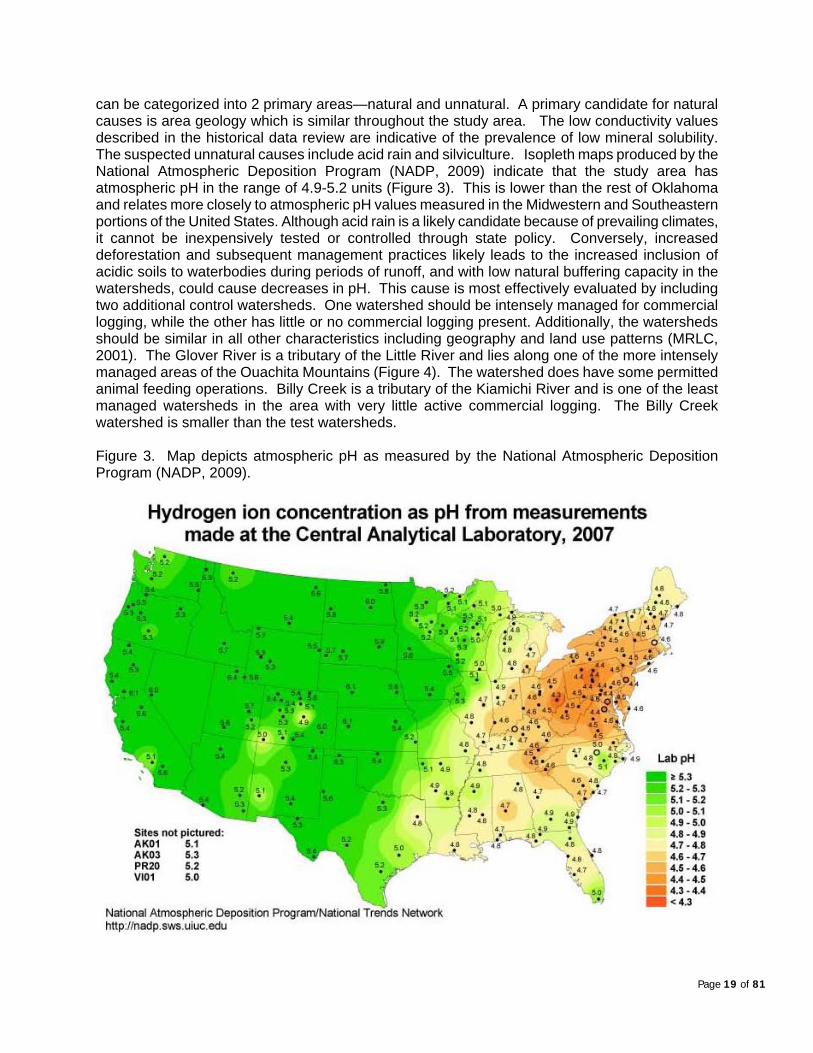
can be categorized into 2 primary areas—natural and unnatural. A primary candidate for natural causes is area geology which is similar throughout the study area. The low conductivity values described in the historical data review are indicative of the prevalence of low mineral solubility. The suspected unnatural causes include acid rain and silviculture. Isopleth maps produced by the National Atmospheric Deposition Program (NADP, 2009) indicate that the study area has atmospheric pH in the range of 4.9-5.2 units (Figure 3). This is lower than the rest of Oklahoma and relates more closely to atmospheric pH values measured in the Midwestern and Southeastern portions of the United States. Although acid rain is a likely candidate because of prevailing climates, it cannot be inexpensively tested or controlled through state policy. Conversely, increased deforestation and subsequent management practices likely leads to the increased inclusion of acidic soils to waterbodies during periods of runoff, and with low natural buffering capacity in the watersheds, could cause decreases in pH. This cause is most effectively evaluated by including two additional control watersheds. One watershed should be intensely managed for commercial logging, while the other has little or no commercial logging present. Additionally, the watersheds should be similar in all other characteristics including geography and land use patterns (MRLC, 2001). The Glover River is a tributary of the Little River and lies along one of the more intensely managed areas of the Ouachita Mountains (Figure 4). The watershed does have some permitted animal feeding operations. Billy Creek is a tributary of the Kiamichi River and is one of the least managed watersheds in the area with very little active commercial logging. The Billy Creek watershed is smaller than the test watersheds. Figure 3. Map depicts atmospheric pH as measured by the National Atmospheric Deposition Program (NADP, 2009).
Page 19 of 81

Figure 4 . Land use category percentages calculated for each control watershed (MRLC, 2001).
2.33
16.08
74.06
3.91 0.06 0.57 2.99 0.010.00
10.0020.0030.0040.0050.0060.0070.0080.00
Porti
on of
Total
Land
Use
(%)
Billy Creek WatershedLand Use Category Percentages
0.135.82
0.26 0.01 0.01
17.51
53.50
11.05
0.705.25 5.34
0.01 0.37 0.040.00
10.00
20.00
30.00
40.00
50.00
60.00
Portio
n of T
otal L
and U
se (%
)
Lower Glover River WatershedLand Use Category Percentages
pH Monitoring. To determine the cause of low pH values, certain water quality parameters and stream stage were continuously collected at stations in each of the study and control watersheds (Table 4). At each location, a data collection platform (DCP) was installed consisting of a Design Analysis Waterlog® datalogger and high data rate GOES radio (OWRB, 2004a). Water quality data were collected using a YSI® 6000EDS multiparameter instrument (sonde) with probes for measuring water temperature, pH, specific conductance, and turbidity (OWRB, 2005b). Using perforated drag tubes made of high-density polyethylene (HDPE), instruments were installed on the downstream side of the bridge near the center channel. To decrease fouling and keep probe surfaces free of foreign material, EDS (extended deployment system) sondes were used because they incorporate a central universal wiping system. Stream stage was collected two different ways. At the Glover, Kiamichi, and Mountain Fork stations, the United States Geological Survey (USGS) manages DCP’s as part of the Oklahoma–USGS cooperative agreement. For these stations, stage data and stage/discharge ratings maintained by the USGS were used. More information for these sites and their equipment can be found at the USGS Oklahoma Water Science Center (http://ok.water.usgs.gov/). At the Little River and Billy Creek stations, stage data were collected
Page 20 of 81

by the OWRB using self contained gas bubbler technology, and the stage/discharge ratings were established by the OWRB using internally collected discharge data (OWRB, 2005a). Data were logged on 15-minute intervals and transmitted hourly via GOES satellite telemetry. Transmitted data were then captured by the United States Army Corps of Engineers (USACE) and redisplayed for public use on the USACE Water Control Homepage.
Calibration and maintenance of the YSI® sondes was performed on alternating two week-three week intervals (OWRB, 2005b). During these service events, several sets of data were collected so that final water quality records could be shifted to account for drift from two sources—fouling and calibration. Initially, all probes (except water temperature) were cleaned with a pre-cleaning and post-cleaning value recorded. The percentage difference between these two readings was applied to all data in the service interval as a fouling correction. After the sensor was cleaned, a calibration check was performed with calibration occurring as needed. When calibration was necessary, a calibration correction was applied to all data in the service interval. To correct data, the sum of the fouling and calibration corrections was applied as a two-point shift over the service interval with the assumption that drift occurred at a constant rate over that interval. The 15-minute corrected data were then averaged into hourly data for further analyses.
Metals Collections. To supplement data collection efforts for the study, collections were made for certain metals throughout the study watersheds (Table 5). Additionally, hardness values were collected during each sampling event so that metals criteria could be calculated. At each site, five to six collections were made to represent different seasons as well as different flow regimes. Each collection was analyzed for both the total recoverable concentration of the analyte as well as the dissolved fraction. Table 5. Stations for metals analyses. (* denotes BUMP station)
Waterbody ID Waterbody Name County Segment Position
OK410210080010 00 Glover River near Bethel McCurtain Upper to Middle OK410210080010_00 Glover River near Glover* McCurtain Lower OK410310020010_10 Kiamichi River near Big Cedar* LeFlore Upper to Middle OK410310020010_10 Kiamichi River near Muse LeFlore Lower OK410210020140_00 Little River near Nashoba Pushmataha Upper to Middle OK410210020140_00 Little River near Cloudy* Pushmataha Lower OK410210060010_10 Mountain Fork River near Zafra McCurtain Upper OK410210060010 10 Mountain Fork River near Smithville* McCurtain Middle to Lower
Samples were collected by one of three methods—composite, grab, or combination (OWRB, 2006b). The default and most representative method is the composite sample, which accumulates a composited sample made up of 5-10 sub-samples collected across the horizontal and the vertical profile of the stream. The method accounts for both the horizontal and vertical variability in moving waters by using a combination of the depth integration (D-I) method (vertical profile) and the equal-width increment (EWI) method (horizontal profile). The EWI method divides the stream into at 5 to 10 equal increments, depending on wetted width. At each increment, a subsample is collected using the D-I method. The sub-sample is representative of the vertical profile because it collects through the water column at a consistent rate. As the sub-sample is collected, air in the container is
Page 21 of 81

compressed so that the pressure balances the hydrostatic pressure at the air exhaust and the inflow velocity is approximately equal to the stream velocity. Each subsample is collected into a clean polyethylene collection bottle attached to a sediment sampler—the US D-95 for bridge collections or the US DH-81 for wading—and composited into a bagged polyethylene splitter churn. From this composite water, separate aliquots were collected into 1-liter polyethylene bottles for total recoverable and dissolved fraction analyses. Samples were returned to the ODEQ State Environmental Laboratory for both filtering and preservation. All analyses were done in accordance with the ODEQ’s Quality Management Plan (QTRACK No. 00-182) (ODEQ, 2007). While at the site, a separate aliquot was collected from the churn and total hardness was analyzed using a Hach© digital titrator and test kit.
Biological Collections. Criteria for both pH and metals are included in the fish and wildlife propagation beneficial use of the OWQS (OWRB, 2007). For that reason, it is important to quantify ecological health as supplemental analysis to determine if pH or metals are impairing the use. Accordingly, multi-assemblage biological collections were made at nine stations and are included in this study (Table 6). Assemblages include aquatic macroinvertebrates and fish and were collected in accordance with Oklahoma’s Rapid Bioassessment Protocols (RBP) (OWRB, 1999) and the OWRB’s biological collection protocols (OWRB, 2004 and 2006a). Collections were made on either a 400- or 800-meter reach depending on an averaged wetted width. Table 6. Stations sampled for overall biological health analyses. (* denotes BUMP station)
Waterbody ID Waterbody Name County Segment Position
OK410310020070_00 Billy Creek near Muse LeFlore Lower OK410210080010_00 Glover River near Bethel McCurtain Upper to Middle OK410210080010_00 Glover River near Glover* McCurtain Lower OK410310020010_10 Kiamichi River near Big Cedar* LeFlore Upper to Middle OK410310020010 10 Kiamichi River near Muse LeFlore Lower OK410210020140_00 Little River near Cloudy* Pushmataha Lower OK410210020140 00 Little River near Nashoba Pushmataha Upper to Middle OK410210060010_10 Mountain Fork River near Smithville* McCurtain Middle to Lower OK410210060010_10 Mountain Fork River near Zafra McCurtain Upper
A representative fish collection was made at seven of the study sites. Fish were primarily collected using a pram or boat electrofishing unit depending on wadeability. Each fishing unit consisted of a Smith-Root 2.5 generator powered pulsator (GPP) attached to a 3000W Honda generator, and were operated with AC output current at 2-4 amps. Using two netters with ¼ inch mesh dipnets, collections were made in an upstream direction with a target effort of 2000-4000 units depending on reach length. When habitats existed that could not be effectively electrofished, supplemental collections were made using 6’ X 10’ seines of ¼ inch mesh equipped with 8’ brailes. Fish were processed at several intervals during each collection. Fish that were too large for preservation and/or readily identifiable were field identified to species and enumerated along with appropriate photodocumentation and representative vouchers. All other fish were preserved in a 10% formalin solution and sent to the University of Oklahoma Sam Noble Museum of Natural History (OUSNMNH) for identification to species and enumeration.
Page 22 of 81

During the summer index period, a representative aquatic macroinvertebrate collection was made at seven of the study sites. Each sampling event targeted three habitats—streamside vegetation, wood, and rocky riffles—that theoretically should be species rich. The streamside vegetation and wood collections were semi-qualitative samples collected over flowing portions of the reach for total collection times of three and five minutes, respectively. The streamside sample was collected using a 500-micron D-frame net to agitate various types of fine structure sample including fine roots, algae, and emergent and overhanging vegetation. Likewise, the wood sample was collected using a 500-micron D-frame net to agitate, scrape, and brush wood of any size in various states of decay. Additionally, wood that could be removed from the stream was scanned for additional organisms outside the 5-minute sampling time. The riffle collection was a quantitative sample compositing three kicks representing slow, medium and fast velocity rocky riffles within the reach. Each sub-sample was collected by fully kicking one square meter into a 500-micron Zo seine. All samples were field post-processed in a 500-micron sieve bucket to remove large material and silt in an effort to reduce sample size to fill no more than ¾ of a quart sample jar. Additionally, all nets and buckets were thoroughly scanned to ensure that no organisms were lost. After processing, each sample type was preserved independently in quart wide mouth polypropylene jars with ethanol and interior and exterior labels were added. Prior to taxonomic analysis, all samples were laboratory processed to obtain a representative 100-count subsample (OWRB, 2006a). After sorting, the “100-count subsample” was sent to EcoAnalysts, Inc. for identification and enumeration, and the large and rare sample was identified and enumerated by OWRB staff. Taxonomic data for each sample were grouped by EcoAnalysts and metrics were calculated. In general, most organisms are identified to genera with midges identified to tribe.
Page 23 of 81

RESULTS
Continuous Data Collection Analysis—All Daily Data. The primary objective of the study is to determine the cause of low pH values throughout the area. As is noted in Table 1, twenty-two waterbodies throughout the study area are listed for pH as category 5a waterbodies in Oklahoma’s 2008 Integrated Report (ODEQ, 2008), including 2 study stations—the Kiamichi River (OK410310020010_10) and Little River (OK410210020140_00). Additionally, eight of the waterbodies listed for pH are co-listed for turbidity. Three possible causes exist for low pH in the area including acid rain (Figure 3), runoff from silviculture activities, and low mineral solubility. Investigating acid rain as a cause is neither cost-effective nor easy, and cannot be controlled through state regulatory measures. Conversely, the other potential causes can be investigated by determining if a relationship exists between increased turbidity or decreased conductivity and decreased pH. As a precursor to regression analysis, it is important to perform some basic analyses of the continuous datasets as well as some historical discrete collections. Recent and available discrete data from all of the lotic stations listed for pH were compiled and descriptive statistics calculated (Table 7). Continuous data were analyzed in a similar fashion. For each of the continuous parameters, both mean and median daily values were calculated from the averaged hourly pH, conductivity, stage, turbidity, and water temperature data. Only mean daily values were calculated for discharge. For each station, descriptive statistics were calculated for all daily parameter means and medians (Table 8). Several of the results are of interest to this study. First of all, the protocol for listing pH requires greater than 10% of all values fall below the minimum criterion of 6.5 (OWRB, 2008a). Both the 10 h and 25th percentile of pH data indicate that multiple listings are probable for much of the watershed, and that the study stations on the Kiamichi River, Little River, and Billy Creek regularly experienced pH values below the criterion. Secondly, the protocol for listing turbidity requires that only 10.6% of all values fall above the criterion of 10 NTU for cool water aquatic communities (CWAC) and 50 NTU for warm water aquatic communities (WWAC) (OWRB, 2008a). Both the mean and 75th percentile of turbidity data indicated that multiple listings are probable. For CWAC stations on the Glover River, Little River, and Mountain Fork River, both median and 75th percentile indicate turbidity values were above the allowable level of 10 NTU. Conversely, WWAC watersheds (Kiamichi River and Billy Creek) do not approach impairment status, but the Billy Creek upper quartile and median are similar to the CWAC study stations. Thirdly, the interquartile range of conductivity for both datasets is somewhere in the area 10 – 65 uS/cm, which is indicative of low mineralization throughout the watersheds. Lastly, stage and discharge data at continuous stations indicate that most of the region received some elevated runoff during the study period. Table 7. Descriptive statistics of chemical variables considered for historical data review.
Statistic pH (units) Conductivity (uS) Turbidity (NTU)
Water Temperature (oC)
n 403.00 210.00 210.00 430.00mean 7.07 31.22 13.84 17.61p10 6.33 10.00 3.00 8.00p25 6.69 10.78 5.00 10.60p50 7.07 27.05 8.00 16.50p75 7.46 42.75 15.00 24.50min 5.01 10.00 1.00 3.10max 8.75 102.00 173.00 34.11
Page 24 of 81
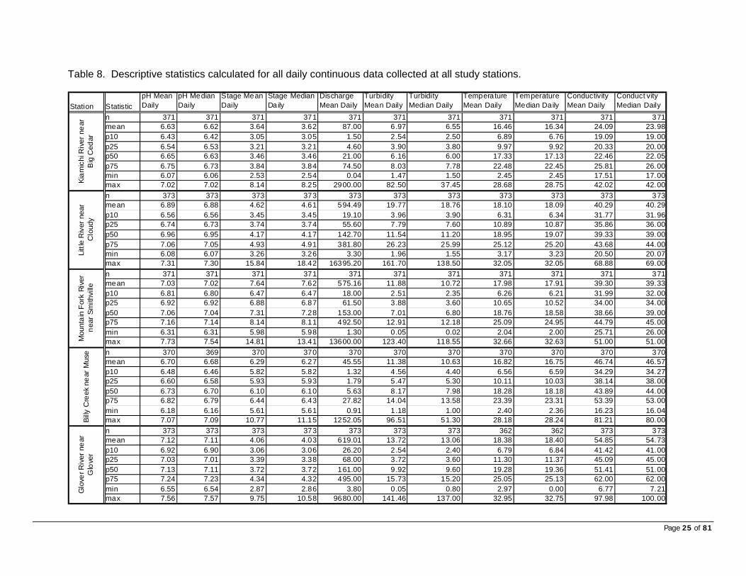
Table 8. Descriptive statistics calculated for all daily continuous data collected at all study stations.
Station StatisticpH Mean Daily
pH Median Daily
Stage Mean Daily
Stage Median Daily
Discharge Mean Daily
Turbidity Mean Daily
Turbidity Median Daily
Temperature Mean Daily
Temperature Median Daily
Conductivity Mean Daily
Conduct vity Median Daily
n 371 371 371 371 371 371 371 371 371 371 371mean 6.63 6.62 3.64 3.62 87.00 6.97 6.55 16.46 16.34 24.09 23.98p10 6.43 6.42 3.05 3.05 1.50 2.54 2.50 6.89 6.76 19.09 19.00p25 6.54 6.53 3.21 3.21 4.60 3.90 3.80 9.97 9.92 20.33 20.00p50 6.65 6.63 3.46 3.46 21.00 6.16 6.00 17.33 17.13 22.46 22.05p75 6.75 6.73 3.84 3.84 74.50 8.03 7.78 22.48 22.45 25.81 26.00min 6.07 6.06 2.53 2.54 0.04 1.47 1.50 2.45 2.45 17.51 17.00max 7.02 7.02 8.14 8.25 2900.00 82.50 37.45 28.68 28.75 42.02 42.00n 373 373 373 373 373 373 373 373 373 373 373mean 6.89 6.88 4.62 4.61 594.49 19.77 18.76 18.10 18.09 40.29 40.29p10 6.56 6.56 3.45 3.45 19.10 3.96 3.90 6.31 6.34 31.77 31.96p25 6.74 6.73 3.74 3.74 55.60 7.79 7.60 10.89 10.87 35.86 36.00p50 6.96 6.95 4.17 4.17 142.70 11.54 11.20 18.95 19.07 39.33 39.00p75 7.06 7.05 4.93 4.91 381.80 26.23 25.99 25.12 25.20 43.68 44.00min 6.08 6.07 3.26 3.26 3.30 1.96 1.55 3.17 3.23 20.50 20.07max 7.31 7.30 15.84 18.42 16395.20 161.70 138.50 32.05 32.05 68.88 69.00n 371 371 371 371 371 371 371 371 371 371 371mean 7.03 7.02 7.64 7.62 575.16 11.88 10.72 17.98 17.91 39.30 39.33p10 6.81 6.80 6.47 6.47 18.00 2.51 2.35 6.26 6.21 31.99 32.00p25 6.92 6.92 6.88 6.87 61.50 3.88 3.60 10.65 10.52 34.00 34.00p50 7.06 7.04 7.31 7.28 153.00 7.01 6.80 18.76 18.58 38.66 39.00p75 7.16 7.14 8.14 8.11 492.50 12.91 12.18 25.09 24.95 44.79 45.00min 6.31 6.31 5.98 5.98 1.30 0.05 0.02 2.04 2.00 25.71 26.00max 7.73 7.54 14.81 13.41 13600.00 123.40 118.55 32.66 32.63 51.00 51.00n 370 369 370 370 370 370 370 370 370 370 370mean 6.70 6.68 6.29 6.27 45.55 11.38 10.63 16.82 16.75 46.74 46.57p10 6.48 6.46 5.82 5.82 1.32 4.56 4.40 6.56 6.59 34.29 34.27p25 6.60 6.58 5.93 5.93 1.79 5.47 5.30 10.11 10.03 38.14 38.00p50 6.73 6.70 6.10 6.10 5.63 8.17 7.98 18.28 18.18 43.89 44.00p75 6.82 6.79 6.44 6.43 27.82 14.04 13.58 23.39 23.31 53.39 53.00min 6.18 6.16 5.61 5.61 0.91 1.18 1.00 2.40 2.36 16.23 16.04max 7.07 7.09 10.77 11.15 1252.05 96.51 51.30 28.18 28.24 81.21 80.00n 373 373 373 373 373 373 373 362 362 373 373mean 7.12 7.11 4.06 4.03 619.01 13.72 13.06 18.38 18.40 54.85 54.73p10 6.92 6.90 3.06 3.06 26.20 2.54 2.40 6.79 6.84 41.42 41.00p25 7.03 7.01 3.39 3.38 68.00 3.72 3.60 11.30 11.37 45.09 45.00p50 7.13 7.11 3.72 3.72 161.00 9.92 9.60 19.28 19.36 51.41 51.00p75 7.24 7.23 4.34 4.32 495.00 15.73 15.20 25.05 25.13 62.00 62.00min 6.55 6.54 2.87 2.86 3.80 0.05 0.80 2.97 0.00 6.77 7.21max 7.56 7.57 9.75 10.58 9680.00 141.46 137.00 32.95 32.75 97.98 100.00
Kiam
ichi
Riv
er n
ear
Big
Ced
arLi
ttle
Riv
er n
ear
Clo
udy
Glo
ver R
iver
nea
r G
love
rM
ount
ain
Fork
Riv
er
near
Sm
ithvi
lleBi
lly C
reek
nea
r Mus
e
Page 25 of 81

At each continuous station, intensive regression analyses were performed to determine the relationship of pH to conductivity, discharge, stage, and turbidity. The three objectives of the analyses were to:
• Determine the best explanatory model for pH using multiple linear regressions (MLR). • Based on the MLR and simple linear regression best fits, determine the most predictive
individual variable for each model. • Based on the MLR and simple linear regression best fits, determine whether conductivity or
turbidity is the best predictor of pH. Before regression progressed, data were analyzed to determine what data to use and in what form. The pH data were evaluated to verify that data were normally distributed, and then to determine whether daily means and/or medians should be used in the model. To investigate data distribution, a series of probability plots were created for daily mean and median pH data at each station (Figure 5 and Figure 6). With the exception of the Muse station, all plots show near normal distributions for both daily means and medians. The data fall outside of the 95% confidence interval at both lower and upper tails, but the tailings of the distributions tend to hold even when data are lognormally transformed. Muse is the only exception with daily median data showing a highly abnormal distribution, which could not be lognormally transformed by the statistical package. Several other data transformations were performed with the same end result (not graphically included but available upon request). Based on this analysis, it was determined that data transformation was unnecessary and would not add to a better fit regression model. To determine whether daily means and/or medians should be used in the analysis, box plots of both data sets were created for all stations (Figure 7). With few minor exceptions, daily mean and median data sets were nearly equal for all stations. This is further visualized by comparing the descriptive statistics in Table 8. Differences between the mean and median data are most often in the hundredths of a unit. The minor exceptions to this rule include a higher maximum value for Smithville daily mean and a slightly tighter interquartile range for the Muse daily median. Assuming that the data used to create these distributions are temporally equivalent, only one of the daily pH data sets should be required in analysis. This assumption was vetted by performing side by side regressions with the daily mean and median data sets in early regression analyses (data analysis available upon request). Typically, regression models produced near equivalent results for both daily data sets. For some analyses, the mean daily data produced a better fit model, presumably because the use of the median muted the effects of days with some more extreme pH swings. Therefore, non-transformed mean daily pH data were used to calculate all regression models. The Minitab© version 15.0 (2007) software was used to produce all probability plots and boxplots as well as run all subsequent regression analyses, including model selection and development. A logical follow-up to the pH data analyses was to expose predictor variables to the same scrutiny. The possible number of predictors available for analysis was 18. This included 5 variables (stage, discharge, conductivity, turbidity, and water temperature) with both daily mean and median values (except discharge) of which each could be transformed or non-transformed. To investigate data distribution, a series of probability plots were created for all variable daily mean and median data at each station (Figures 8-12). All non-transformed data appear to have some abnormality in distribution. This is further visualized in the box plots provided for stage (Figure 13), conductivity (Figure 16), turbidity (Figure 14), and water temperature (Figure 15). The cause of abnormality for stage, conductivity, and turbidity is largely influenced by values tailing to the right of the distribution. Conversely, water temperature is largely influenced by an extended interquartile range resulting in a platykurtic distribution. Discharge demonstrates a typical leptokurtic distribution with large tails to the left and right of the median. Discharge, conductivity, and turbidity tend toward a more normal distribution when data are log transformed. On the other hand, stage continues to tail in both
Page 26 of 81

Figure 5. Probability plots represent the normal and lognormal distributions of pH mean and median dailies for the Kiamichi River near Big Cedar, Little River near Cloudy, and Mountain Fork River near Smithville.
Page 27 of 81

Figure 6. Probability plots represent the normal and lognormal distribution of pH mean and median dailies for the Glover River near Glover and Billy Creek near Muse.
Page 28 of 81

Page 29 of 81
Figure 7. Boxplots represent daily pH means and medians for all continuous data.

directions, while water temperature remains influenced by the right tail of the distribution. Based on this analysis and in the interest of a fair and equitable vetting of all data, each predictor remained as a possible model predictor for the study. Before the best multiple linear regression models could be selected for each station, several steps were taken to select the best model predictors for each station. Helsel and Hirsch (1995) recommend “a cost-benefit analysis” to aid in determining whether variables “sufficiently improve(s) the model.” First, a best subsets analysis was performed. Free predictors included all possible parameters including mean and median dailies that have been log-transformed and non-transformed. No variables were used as a predictor in all models. Subsets were run for all possible predictor combinations with the top five combinations at each grouping level graphically displayed in the model output. Each subset produced several statistics including the R2 value and the standard error (s). Additionally, several overall measures of quality were calculated to assist in evaluating the subsets, including the adjusted R2 and Mallow’s Cp. The adjusted R2 accounts for the number of explanatory predictors in each subset. The closer it is to R2, the better the model. Mallow’s Cp accounts for two of the competing desires in model selection—explaining variation and minimizing the standard error. Typically, the Mallow’s Cp value can be evaluated by looking for the lowest value of all the predicted subsets or by looking for the value that is closest to the number of predictors plus the constant. Because of the sheer volume of information, best subset regression outputs are not included in the report but are available upon request. A second procedure used to aid in selection of best predictors was stepwise regression. The process adds and removes individual predictors testing for significance (preset at 0.15) as an individual predictor and in the context of the growing model (Helsel and Hirsch, 1995). Several measures of quality are produced for each model, including the adjusted R2, Mallow’s Cp, the prediction sum of squares (PRESS), and the predicted R2. The PRESS and predicted R2 assess overall model fit. As the predicted R2 moves closer to R2 and adjusted R2 and as PRESS becomes lower, a model is considered to have better predictive ability. The resulting predictor analyses led to variable results for study stations, and in some cases produced erratic results from the two models, specifically for water temperature. Inevitably, a matrix of all model predictors was created. Multiple linear regressions were run for all combinations of predictor groups, and best predictive models were chosen. With the best predictive models chosen for each station, final regression analyses were ran in a 2-step process for each study station. First, simple linear regression was performed for individual parameters versus mean daily pH. The best fit lines for parameters not included in MLR models are available upon request. For parameters used in the best-fit MLR models, best fit lines are presented and discussed in the main body of the report. Secondly, the general linear model for regression was performed using best predictors. The model included several outputs to account for predictor and model significance as well as demonstrate the overall model fit. To verify that intercept and slope coefficients were not equal to zero, a t-ratio was calculated for each term, and only those with p-values < 0.05 were considered significant. To evaluate individual predictor fit, the procedure calculated the sequential sum of squares and variance inflation factor (VIF). Generally, the higher sequential sum of squares value indicated more predictive ability and was compared between predictors (Minitab, 2007). The VIF was used to determine predictor multi-collinearity or the inflation of term’s predictive ability because of some degree of correlation to another predictor. Though undocumented in statistical texts, a VIF greater than 10 is generally considered worrisome and predictors should be evaluated (Minitab, 2008). Model significance (p-value < 0.05) was evaluated using analysis of variance (ANOVA). The R2 and adjusted R2 were calculated to demonstrate the amount of variance explained by the model. Model fit was evaluated using predicted R2, Mallow’s Cp, and PRESS.
Page 30 of 81

Figure 8. Probability plots represent the normal and lognormal distributions of variable mean and median dailies for the Kiamichi River near Big Cedar. Variables include stage, discharge (mean only), turbidity, water temperature, and specific conductivity.
Page 31 of 81
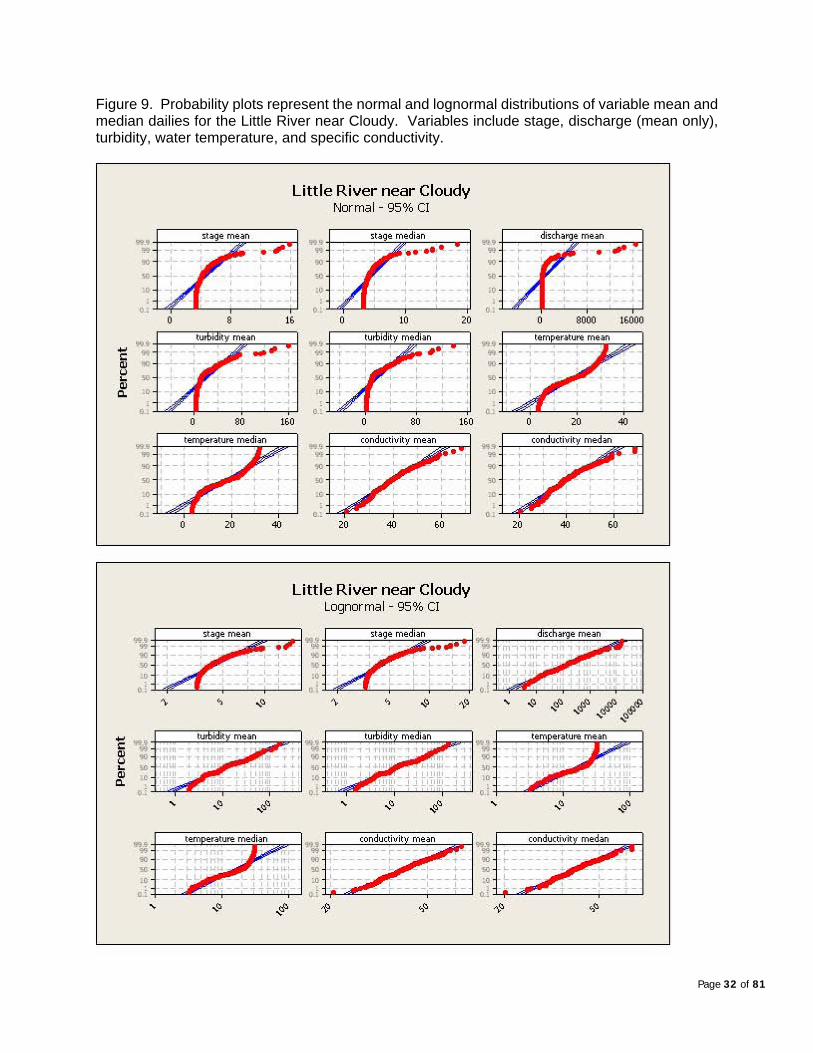
Figure 9. Probability plots represent the normal and lognormal distributions of variable mean and median dailies for the Little River near Cloudy. Variables include stage, discharge (mean only), turbidity, water temperature, and specific conductivity.
Page 32 of 81
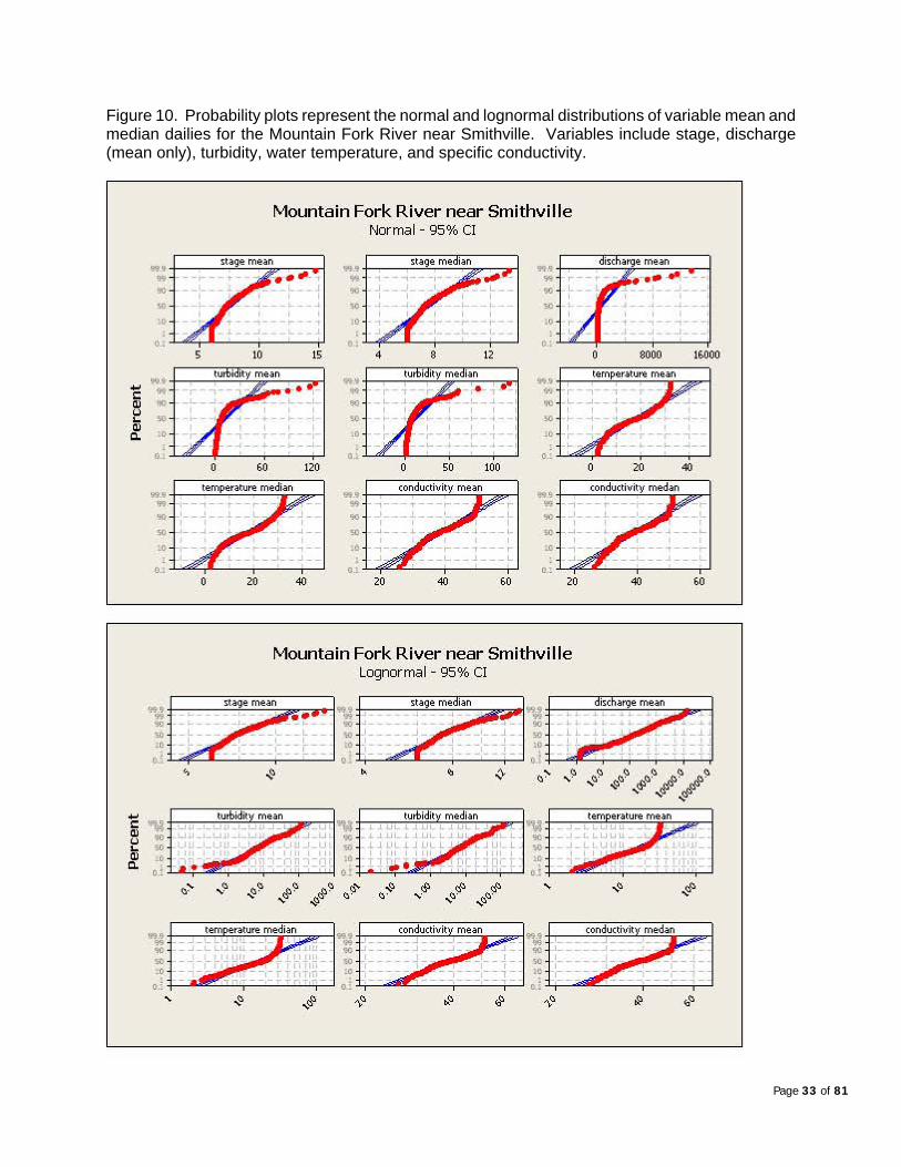
Figure 10. Probability plots represent the normal and lognormal distributions of variable mean and median dailies for the Mountain Fork River near Smithville. Variables include stage, discharge (mean only), turbidity, water temperature, and specific conductivity.
Page 33 of 81

Figure 11. Probability plots represent the normal and lognormal distributions of variable mean and median dailies for the Glover River near Glover. Variables include stage, discharge (mean only), turbidity, water temperature, and specific conductivity.
Page 34 of 81

Figure 12. Probability plots represent the normal and lognormal distributions of variable mean and median dailies for Billy Creek near Muse. Variables include stage, discharge (mean only), turbidity, water temperature, and specific conductivity.
Page 35 of 81

Figure 13. Boxplots represent daily stage means and medians for all continuous data at all stations.
Page 36 of 81
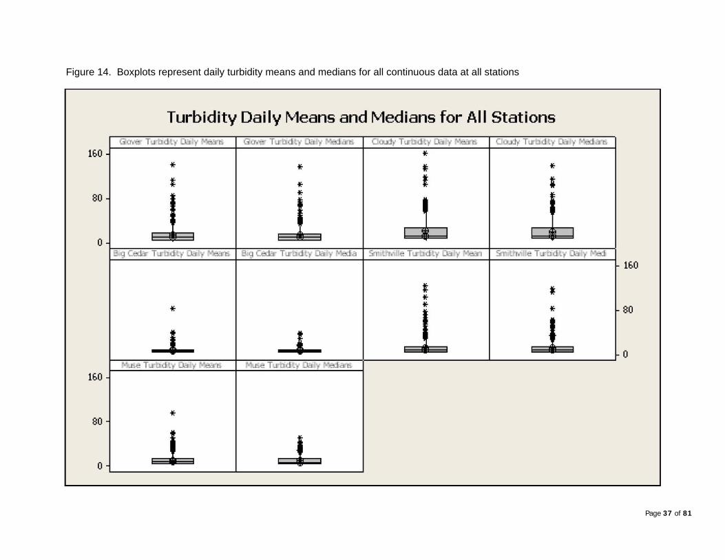
Figure 14. Boxplots represent daily turbidity means and medians for all continuous data at all stations
Page 37 of 81

Figure 15. Boxplots represent daily water temperature means and medians for all continuous data at all stations.
Page 38 of 81

Page 39 of 81
Figure 16. Boxplots represent daily conductivity means and medians for all continuous data at all stations.

After exhaustive evaluation, the best fit multiple linear regression models were determined for all study and control stations. The model for the Kiamichi River near Big Cedar is presented in Table 9. The model is significant and has fair predictive capacity with an R2 of 40.5. It also has an excellent fit with a Mallow’s Cp of 4.0 and PRESS of 5.9. The mean daily pH is best fit by stage, discharge, and conductivity. Stage is the best predictor as evidenced by a high sequential sum of squares of 5.8 compared to 1.0 for other predictors. It also shows good fit as an individual term in simple regression (Figure 17). Although conductivity produces a better model, it is poor as an individual predictor. The likely explanation is that data are heavily distributed to the left tail. However, log normalizing data did not produce a better fit. When turbidity was included in the model, a nearly equivalent amount of variance was explained, but the term was insignificant (p = 0.856). Two equally predictive models were created for the Little River near Cloudy. Both models are significant. The main difference between the models is inclusion of discharge as a predictor in model 2 (Table 11). Both models display excellent predictive ability and fit. However, model 2 explains slightly more variation with an R2 of 71.1 versus 65.5 for model 1 (Table 10). Conversely, both models appear to be equally well fit. In model 2, multi-collinearity of stage and discharge may be of some concern. For both models, stage is the best predictor. The sequential sum of squares are much higher than other terms, and when considering simple regression (Figure 18), stage displays a much better fit. Conductivity appears to be a better predictor than turbidity. The terms have equivalent sequential sum of squares in model 2 but the same predictor of fit in model 1 is more than double for conductivity. Furthermore, when considered as individual terms, conductivity demonstrates a much better explanatory ability with an R2 of 46.2 as compared to 33.6 for turbidity. Results of regression analysis for the Mountain Fork River near Smithville are presented in Table 12. The model is significant with relatively good predictive capacity (R2 = 57.1) and excellent fit (Mallow’s Cp = 5.1 and PRESS = 5.7). The mean daily pH is best fit by stage, discharge, turbidity, and conductivity. As with the other study stations, stage is the best predictor as evidenced by a relatively high sequential sum of squares of 6.9, which is more than 34 times higher than the nearest value. Stage also has high individual explanatory capacity in simple regression (R2 = 53.7) (Figure 19). Conductivity and turbidity look as if they have identical predictive capacity as evidenced by similar sequential sum of squares and nearly equivalent R2 values. The mean daily pH for the Glover River near Glover is best predicted by stage, discharge, conductivity, and turbidity (Table 13). The model is significant but has relatively poor predictive capacity (R2 = 26.3). Likewise, the fit is suspect. The Mallow’s Cp (5.0) is excellent, but the PRESS is relatively high (8.0) and the predicted R2 (21.7) is far below the R2 value. Again, stage is the best predictor although less so than with the other 3 test stations. The sequential sum of squares is relatively low (1.56) as is the R2 of 15.2 (Figure 20). Comparing conductivity and turbidity presents a mixed bag of results. The R2 values are nearly equivalent. However, the sequential sum of squares is over 4 times higher for conductivity (0.60) than for turbidity (0.14). Lastly, data from the regression analysis for Billy Creek near Muse are presented in Table 14. As with Glover, the model is significant but has the poorest predictive capacity of all stations with an R2 of 21.8. However, the fit appears to be much better than with the Glover station. The Mallow’s Cp (4.3) is excellent, as is the predicted R2 of 20.3. However, the PRESS is still relatively high at 8.4. Discharge, conductivity, and turbidity are the best model predictors. Conspicuously, stage is missing from the model. When included, the overall R2 drops to 16.5. Conductivity (R2 = 10.2) is a much better predictor than turbidity (R2 = 0.1) in simple regression analysis (Figure 21).
Page 40 of 81

Table 9. Results generated from multiple linear regression analysis for best whole dataset predictors of mean daily pH at the Kiamichi River near Big Cedar. The best fit predictive equation is: pH Mean Daily = 7.76 - 0.0908 Stage Mean Daily - 0.124 Discharge Mean Daily Log10 - 0.0267 Conductivity Mean Daily. (*** = significant at an alpha < 0.01)
Predictors Regression Coefficients
Standard Error of Coefficient
T Statistic Value P-value
Sequential Sum of Squares
Variance Inflation Factor
Constant 7.7555 0.0782 99.19 * * * Mean Conductivity -0.0908 0.0166 -5.46 * * * 5.8170 3.90Mean Turbidity -0.1240 0.0239 -5.20 * * * 1.0435 10.97Mean Stage Log10 -0.0267 0.0028 -9.45 * * * 1.1414 5.54
Regression Statistics Results of Analysis of Variance
Statistic Value Source Degrees of Freedom
Sum of Squares Mean Square
F Statistic Value
P-value
S 0.13 Regression 3 3.9537 1.3179 83.15 * * *
R2 40.5Residual Error 367 5.8170 0.0159
R2-adjusted 40.0 Total 370 9.7707 R-Sq(predicted) 39.5Mallows Cp 4.0PRESS 5.9
Page 41 of 81

Figure 17. Best fit regression lines represent best whole dataset predictors of mean daily pH at the Kiamichi River near Big Cedar. Best fit lines are depicted for mean daily pH vs. mean daily stage, log10 of mean daily discharge, and mean daily conductivity.
Page 42 of 81

Table 10. Results generated from multiple linear regression analysis for best whole dataset predictors of mean daily pH at the Little River near Cloudy (Model 1). The best fit predictive equation is: pH Mean Daily = 5.54 - 0.0538 Stage Mean Daily - 0.00238 Turbidity Mean Daily + 1.03 Conductivity Median Daily Log10. (*** = significant at alpha < 0.01)
Predictors Regression Coefficients
Standard Error of Coefficient
T Statistic Value P-value
Sequential Sum of Squares
Variance Inflation Factor
Constant 5.5403 0.2141 25.88 * * * Mean Conductivity -0.0538 0.0066 -8.21 * * * 10.933 2.42Mean Turbidity -0.0024 0.0004 -5.79 * * * 0.508 1.57Mean Stage Log10 1.0293 0.1223 8.42 * * * 1.290 1.77
Regression Statistics Results of Analysis of Variance
Statistic Value Source Degrees of Freedom
Sum of Squares Mean Square
F Statistic Value
P-value
S 0.13 Regression 3 12.7310 4.2437 233.06 * * *
R2 65.5Residual Error 369 6.7188 0.0182
R2-adjusted 65.2 Total 372 19.4498 R-Sq(predicted) 63.9Mallows Cp 4.0PRESS 7.0
Page 43 of 81

Table 11. Results generated from multiple linear regression analysis for best whole dataset predictors of mean daily pH at the Little River near Cloudy (Model 2). The best fit predictive equation is: pH Mean Daily = 6.79 - 0.168 Stage Mean Daily + 0.0000944 Discharge Mean Daily - 0.00193 Turbidity Mean Daily + 0.538 Conductivity Median Daily Log10. (*** = significant at alpha < 0.01)
Predictors Regression Coefficients
Standard Error of Coefficient
T Statistic Value P-value
Sequential Sum of Squares
Variance Inflation Factor
Constant 6.7887 0.2447 27.75 * * * Mean Conductivity -0.1679 0.0147 -11.44 * * * 10.9330 14.46Mean Turbidity 0.0001 0.0000 8.52 * * * 2.3035 9.76Mean Stage Log10 -0.0024 0.0004 -5.07 * * * 0.3230 1.60
Regression Statistics Results of Analysis of Variance
Statistic Value Source Degrees of Freedom
Sum of Squares Mean Square
F Statistic Value
P-value
S 0.12 Regression 4 13.8378 3.4595 226.85 * * *
R2 71.1Residual Error 368 5.6120 0.0152
R2-adjusted 70.8 Total 372 19.4498 R-Sq(predicted) 70.3Mallows Cp 5.1PRESS 5.8
Page 44 of 81

Figure 18 . Best fit regression lines represent best whole dataset predictors of mean daily pH at the Little River near Cloudy. Best fit lines are depicted for mean daily pH vs. mean daily stage, mean daily discharge, mean daily turbidity, and the log10 of median daily conductivity.
Page 45 of 81

Table 12. Results generated from multiple linear regression analysis for best whole dataset predictors of mean daily pH at the Mountain Fork near Smithville. The best fit predictive equation is: pH Mean Daily = 6.604 - 1.1112 Stage Mean Daily + 0.0993 Discharge Mean Daily Log 10 - 0.1003 Turbidity Mean Daily Log10 + 0.7225 Conductivity Median Daily. (*** = significant at alpha < 0.01)
Predictors Regression Coefficients
Standard Error of Coefficient
T Statistic Value P-value
Sequential Sum of Squares
Variance Inflation Factor
Constant 6.6040 0.3325 19.86 * * * Mean Conductivity -1.1112 0.0116 -9.63 * * * 6.9509 5.03Mean Turbidity 0.0993 0.0249 4.00 * * * 0.0281 8.88Mean Stage Log10 -0.1003 0.0203 -4.95 * * * 0.1917 2.16
Regression Statistics Results of Analysis of Variance
Statistic Value Source Degrees of Freedom
Sum of Squares Mean Square
F Statistic Value
P-value
S 0.12 Regression 4 7.4013 1.8503 121.97 * * *
R2 57.1Residual Error 366 5.5524 0.0152
R2-adjusted 56.7 Total 370 12.9537 R-Sq(predicted) 56.2Mallows Cp 5.1PRESS 5.7
Page 46 of 81

Figure 19. Best fit regression lines represent best whole dataset predictors of mean daily pH at the Mountain Fork near Smithville. Best fit lines are depicted for mean daily pH vs. mean daily stage, the log10 of mean daily discharge, log10 of mean daily turbidity, and the log 10 of median daily conductivity.
Page 47 of 81

Page 48 of 81
Table 13. Results generated from multiple linear regression analysis for best whole dataset predictors of mean daily pH at the Glover River near Glover. The best fit predictive equation is: pH Mean Daily = 6.98 - 1.83 Stage Mean Daily Log 10 + 0.261 Discharge Mean Daily Log 10 - 0.0725 Turbidity Mean Daily Log10 + 0.419 Conductivity Median Daily Log10. (*** = significant at alpha < 0.01)
Predictors Regression Coefficients
Standard Error of Coefficient
T Statistic Value P-value
Sequential Sum of Squares
Variance Inflation Factor
Constant 6.9750 0.1550 45.00 * * * Mean Conductivity -1.8334 0.2413 -7.60 * * * 1.5565 10.61Mean Turbidity 0.2609 0.0383 6.81 * * * 0.4001 12.88Mean Stage Log10 -0.0725 0.0260 -2.79 * * * 0.1442 2.26
Regression Statistics Results of Analysis of Variance
Statistic Value Source Degrees of Sum of
Squares Mean Square F Statistic Value
P-value Freedom
S 0.14 Regression 4 2.7011 0.6753 32.85 * * *
R2 26.3Residual Error 368 7.5650 0.0206
R2-adjusted 25.5 Total 372 10.2661 R-Sq(predicted) 21.7Mallows Cp 5.0PRESS 8.0

Page 49 of 81
Figure 20. Best fit regression lines represent best whole dataset predictors of mean daily pH at the Glover River near Glover. Best fit lines are depicted for mean daily pH vs. log10 of mean daily stage, the log10 of mean daily discharge, log10 of mean daily turbidity, and the log 10 of median daily conductivity.
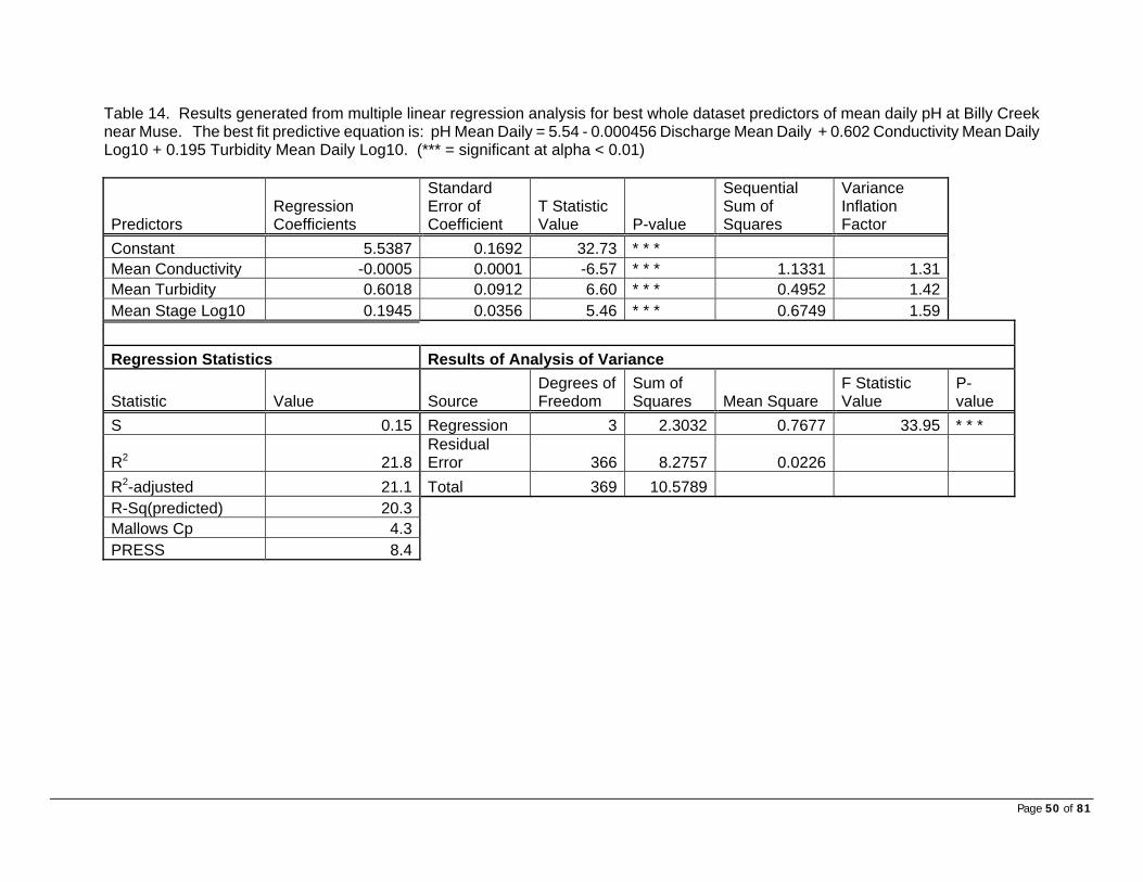
Page 50 of 81
Table 14. Results generated from multiple linear regression analysis for best whole dataset predictors of mean daily pH at Billy Creek near Muse. The best fit predictive equation is: pH Mean Daily = 5.54 - 0.000456 Discharge Mean Daily + 0.602 Conductivity Mean Daily Log10 + 0.195 Turbidity Mean Daily Log10. (*** = significant at alpha < 0.01)
Predictors Regression Coefficients
Standard Error of Coefficient
T Statistic Value P-value
Sequential Sum of Squares
Variance Inflation Factor
Constant 5.5387 0.1692 32.73 * * * Mean Conductivity -0.0005 0.0001 -6.57 * * * 1.1331 1.31Mean Turbidity 0.6018 0.0912 6.60 * * * 0.4952 1.42Mean Stage Log10 0.1945 0.0356 5.46 * * * 0.6749 1.59
Regression Statistics Results of Analysis of Variance
Statistic Value Source Degrees of Freedom
Sum of Squares Mean Square
F Statistic Value
P-value
S 0.15 Regression 3 2.3032 0.7677 33.95 * * *
R2 21.8Residual Error 366 8.2757 0.0226
R2-adjusted 21.1 Total 369 10.5789 R-Sq(predicted) 20.3Mallows Cp 4.3PRESS 8.4
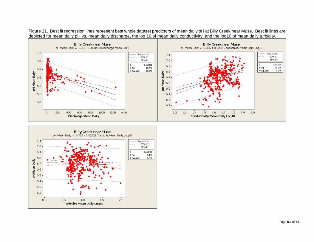
Page 51 of 81
Figure 21. Best fit regression lines represent best whole dataset predictors of mean daily pH at Billy Creek near Muse. Best fit lines are depicted for mean daily pH vs. mean daily discharge, the log 10 of mean daily conductivity, and the log10 of mean daily turbidity.

Page 52 of 81
Continuous Data Collection Analysis—Hourly Data Related to Runoff Events.
ll watersheds, the chemical and physical properties of the study watersheds will change during events. Using the Little River near Cloudy station as a representative of the watershed, time graphs demon e changes. nerally, as runoff increases, turbidity (Table 23) ses while both 22) an co tivity (Figure 24) decrease. Because of these nshi important to determin p ctor/response relationships during runoff events.
is po nalysis, hourly data compiled for each station. Parameters included pH, ctivi nd stream stage. arge s cluded because the upper end of the rating y Creek near Muse is not fully developed. The station was only gauged during the 1-year study and an inadequa of high flo u ents were acquired to construct a rating that is rab other s the study fl ata were separated from the entire dataset h bo liz imple sta ro s. Relative percent differences were calculate the s series. When a greater than 1% rise occurred in stage, data were pulled from the
ded to a “runoff” dataset. These data were then compared to time series graphs noff further refined with some data being further excluded from the analysis. The t was terminated on the downward slope of each runoff event when a zero percent change in occurred e time series data.
estigate of ff” subs roba y plots were created for each er sho l a al distribution o ch at each station. All non-ed and lo d d ea h e abnormality in distribution, with extent ali ry sta aram Furthermore, the tailing of the data that
the also no nt across the datasets. Based on the inconsistent of d ion and in th fair and equitable vetting of all data, each predictor -tra ed and log-tran emained as a possible model predictor for the study.
emain consistent with the p analysis of all daily data, non-transformed pH was the only variab na .
e gre n uld be selected for each station, several steps e t the best mode d ation (Helsel and Hirsch, 1995). First, a se is was performed. Free predictors included all possible parameters including formed and non-transformed values. No variables were used as a predictor in all models. were run for all possible predictor combinations with the top five combinations at each level grap yed in the mo l o subset produced several statistics the R2 tandard error(s). Additionally, several overall measures of quality
cula ssist in evaluating the subsets, including the adjusted R2 and Mallow’s Cp. The R2 accounts for the number of explanatory predictors in each subset. The closer it is to ette odel. Secondly, ste e regression was used to aid in the selection of the icto
se analyses, the best pred r variables were chosen and final regression analyses were 2-step proces r st station. First, simple linear regression was performed for l parameters an ly pH. The best fit lines for parameters not used in the final dels are avail req t. For parame ed in the best-fit MLR models, best fit presen ed e main body o rt.
Like arunoff seriesincrearelatio
For thcondufor Billperiodcompathrougalong main data and rudatasestage To invparamettransformof abnormis effect patterns (both nonAlso, to rresponse Before thwere takbest sublog-transSubsets groupingincludingwere caladjustedR2, the bbest pred
From theran in a individuaMLR molines are
strapH
te (Ta
thesble
Genducredi
d e the
were Disch
ps, it is
rtion of aty, turbidity, a wa ex
te ntatioatio
umns
n a
ber in nd s
w m. Htistic
easigh al p
remow dces
le toth a visuatage timeset and ad events were
in th
datawing
d th
istre
ibunor
tionma
thend lata ationt coteresforrior
lysis
ssiol pre
“runoognorm
et, p bilitf ea
g-tringutio
ans ben is
fortwe
meen
pps and pnsistest of amed) r
r to ave ete
somrs. ty va
distribistributnsform
e in
le u
best muln to selects analys
se
tip
d in
le li
th
nea
is a
r re moictor
des f
ls coor each st
hiclue
ally an
did th
splae s
de utput. Each va
ted to a
r the mrs.
pwis
ictoudy daiues
in th
s fo verabled d
each me
ponuss
sus uisc
terf th
s use rted an epo

Page 53 of 81
Fig
ure 22. Time Series represents mean daily stage and pH at the Little River near Cloudy.
Figure
23. Time Series represents mean daily stage and turbidity at the Little River near Cloudy.

Page 54 of 81
Figure 24. Time Series represents mean daily stage and conductivity at the Little River near Cloudy.
Secondly, the general linear model for regression was performed using the best predictors. The model included several outputs to account for predictor and model significance as well as
emonstrate the overall model fit. To verify that intercept and slope coefficients were not equal to
ity, and log10 stage. Turbidity is the best predictor as evidenced by the higher sequential sum of squares of 4.2 compared to < 1.0 for other predictors. However, turbidity
d is comparable to the whole dataset models (R = 71.1 and 65.5). As with the whole dataset model, stage is the best predictor with a simple regression R2 of 56.1 (Figure 26). The R2 values produced by simple regression also indicate that conductivity (R2= 38.9) is a better predictor than turbidity (R2= 24.5). This is further
dzero, a t-ratio was calculated for each term, and only those with p-values < 0.05 were considered significant. To evaluate individual predictor fit, the procedure calculated the sequential sum of squares and variance inflation factor (VIF). Model significance (p-value < 0.05) was evaluated using analysis of variance (ANOVA). The R2 and adjusted R2 were calculated to demonstrate the amount of variance explained by the model. Model fit was evaluated using predicted R2, Mallow’s Cp, and PRESS. The model for the Kiamichi River near Big Cedar is presented in Table 15. The model is significant but has relatively low predictive capacity (R2=19.2) when compared with model for all daily data (R2=40.5). It also has a poor fit with a Mallow’s Cp of 88.7. The mean daily pH is best fit by conductivity, turbid
demonstrates poor predictive capacity as an individual term in simple regression (Figure 25). Both conductivity and stage are very poor predictors. The MLR model for the Little River near Cloudy showed both good predictive ability and fit (Table 16). The model is significant with a relatively high R2 of 66.4 an
2
Page 55 of 81
nd similar to results for the whole dataset MLR model. However, the subset model does show poor
fit with a Mallow’s Cp of 104.8 and a PRESS of 29.2. Results of regression analysis for the Mountain Fork River near Smithville are presented in Table 17. Unlike the whole dataset model (R2 = 57.1), the subset model has relatively low predictive capacity with an R2 of 21.0. The difference is model fit is also apparent. The whole data model had excellent fit (Mallow’s Cp = 5.1 and PRESS = 5.7) compared to the subset model, which had a Mallow’s Cp of 42.8 and a PRESS of 71.4. Conductivity appears to be a better predictor than turbidity, but both have very poor predictive capacity as indicated by simple regression (Figure 27). Although significant in the MLR model, stage has very little predictive capacity with an R2 of 1.2 in simple regression. Conversely, the “runoff” subset model for the Glover River near Glover (Table 18) has relatively high predictive capacity (R2 = 45.0) as compared to the whole data model (R2 = 26.3). However, the fit is much poorer than what was produced by the whole data model (Mallow’s Cp = 5.0 and PRESS = 8.0). Comparative values for the subset model are a Mallow’s Cp > 150.0 and PRESS of 55.5. Conductivity (R2 = 36.7) and turbidity (R2 = 38.9) are nearly equal as predictors in simple regression (Figure 28). However, conductivity potentially demonstrates more predictive capacity with a much higher sequential sum of squares of 36.6 compared to 8.1 for turbidity. Stage is a very poor predictor (R2 = 0.1). Lastly, data from the regression analysis for Billy Creek near Muse are presented in Table 19. Unlike the whole data model (R2=21.8), the subset model has relatively high predictive capacity with an R2 of 64.7. However, the fit is more suspect with a Mallows Cp of 31.4 compared to 4.3 and
RESS of 13.8 compared to 8.4. Conductivity (R2=49.9) and stage (R2=49.6) are the best model
idenced by a much higher sequential sum of squares of 19.3 compared to 5.6 for stage. Although significant in the MLR model, turbidity (R2 = 3.2) showed little predictive capacity in simple regression analysis.
evidenced by the conductivity sequential sum of squares of 33.6 compared to 14.9 for turbidity, ais
a Ppredictors in simple regression (Figure 29), but conductivity may have better predictive capacity as ev
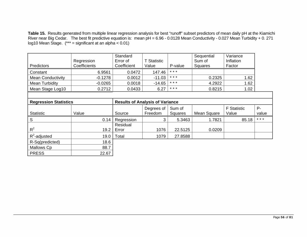
Page 56 of 81
T lt l lysis for best “runoff” subset predictors of mean daily pH at the KiamR e e pH = 6.96 - 0.0128 Mean Conductivity - 0.027 Mean Turbidity + 0. 2lo g t
T Statistic Value P-value
Sequential Sum of Squares
Variance Inflation Factor
able 15. Resuiver near Big Cg10 Mean Sta
Predictors
s generated from mudar. The best fit pr
e. (*** = significant a
Regression Coefficients
tiple linear regresdictive equation is an alpha < 0.01)
StandarError of Coeffici
sion ana: mean
d
ent
ichi 71
Constant 6.9 147.46 * * * 561 0.0472Mean Conductiv -0.1 -11.03 * * * 0.2325 1.62ity 278 0.0012Mean Turbidity -0.0 -14.65 * * * 4.2922 1.62265 0.0018Mean Stage Log 0.2 6.27 * * * 0.8215 1.0210 712 0.0433
Regression Sta ysis of Variance tistics Results of Anal
Statistic Value Source Degrees of Freedom
Sum of Squares Mean Square
F Statistic Value
P-value
S 0.14 Regression 3 5.3463 1.7821 85.18 * * *
R2 19.2ResiduaError
l 1076 22.5125 0.0209
R2-adjusted 19.0 Total 1079 27.8588 R-Sq(predicted) 18.6Mallows Cp 88.7PRESS 2 2.67

Page 57 of 81
Figure 25. Best fit regression lines represent best “runof m m dafit lines are depicted for mean pH vs. mean conductivity, a
f” subset predictors of mean turbidity, and me
ean daily pH at the Kian stage log10.
ichi River near Big Ce r. Best

Page 58 of 81
Table 16. Results generated from multiple linear regression analysis for best “runoff” subset predictors of mean daily pH at the Little Rivenear Cloudy. The best fit predictive equation is: pH Mean Daily = 7.06 + 0.011 Mean Conductivity - 0.190 Mean Turbidity Log10 - 0.676 Mean Stage Log10. (*** = significant at an alpha < 0.01)
r
n s
Predictors RegressioCoefficient
Standard Error of Coefficient
T Statistic Value P-value
Sequential Sum of Squares
Variance Inflation Factor
Constant 7.0504 0.0420 167.99 * * * Mean Conductivity 0.0105 0.0007 15.81 * * * 33.643 1.67Mean Turbidity Log 10 -0.1904 0.0116 -16.41 * * * 14.942 1.22Mean Stage Log10 -0.6755 0.0320 -21.11 * * * 8.845 1.95
Regression Statistics Results of Analysis of Variance
Statistic Value Source Degrees of Freedom
Sum of Squares Mean Square
F Statistic Value
P-value
S 0.14 Regression 3 57.429 19.143 964.10 * * *
R2 66.4Residual Error 1466 29.109 0.020
R2-adjusted 66.3 Total 1469 86.538 R-Sq(predicted) 66.2Mallows Cp 104.8PRESS 29.27
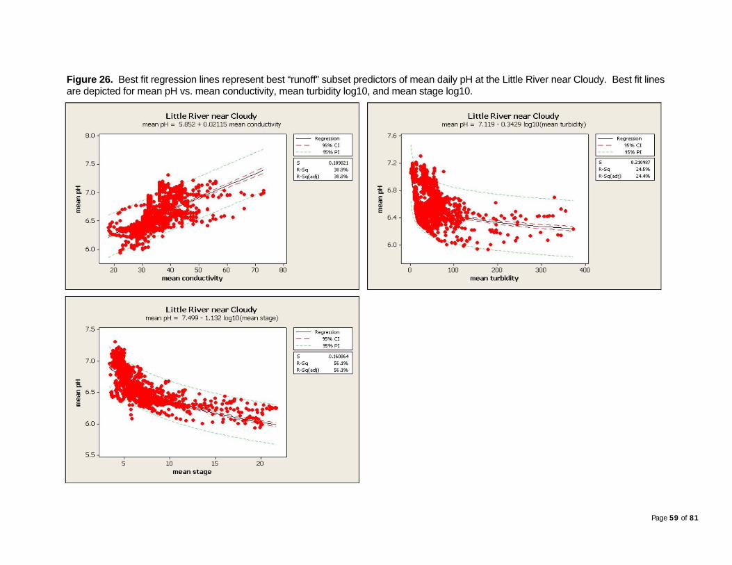
Figure 26. Best fit regression lines represent best “runoff” subset predictors of mean daily pH at the Little River near Cloudy. Best fit lines are depicted for mean pH vs. mean conductivity, mean turbidity log10, and mean stage log10.
Page 59 of 81

Page 60 of 81
Table 17. Results generated from multiple linear regression analysis for best “runoff” subset predictors of mean daily pH at the Mountain
Predictors Regression
nts
Standard T Statistic
P-value
Sequential Variance
Fork River near Smithville. The best fit predictive equation is: pH Mean Daily = 4.77 + 1.12 Mean Conductivity Log10 - 0.003 Mean Turbidity + 0.578 Mean Stage Log10. (*** = significant at an alpha < 0.01)
CoefficieError of Coefficient Value
Sum of Squares
Inflation Factor
Constant 4.7723 31.760.1503 * * * Mean Conductivity Log10 11.806 1.121.1196 0.0762 14.70 * * * Mean Turbidity -0.0034 0.0003 -10.50 * * * 4.549 1.09Mean Stage Log10 0.5776 0.0719 8.03 * * * 2.571 1.03
Regression Statistics Results of Analy is of Variance s
Statistic Value Source Mean Square F Statistic P-
value Degrees of Sum of Freedom Squares Value
S 0.20 3 158.32Regression 18.926 6.309 * * *
R2 21.0 1786 71.169 0.040 Residual Error
R2-adjusted 20.9 Total 1789 90.094 R-Sq(predicted) 20.7Mallows Cp 42.8PRESS 71.4

Figure 27. Best fit regression lines represent best “runoff” subset predictors of mean daily pH at the Mountain Fork River near Smithville. Best fit lines are depicted for mean pH vs. mean conductivity log10, mean turbidity, and mean stage log10.
Page 61 of 81

Page 62 of 81
Table 18. Results generated from multiple linear regression analysis for best “runoff” subset predictors of mean daily pH at the Glover River near Glover. The best fit predictive equation is: pH Mean Daily = 6.02 + 0.721 Mean Conductivity Log10 - 0.175 Mean Turbidity Log10 + 0.007 Mean Stage. (*** = significant at an alpha < 0.01)
Predictors Regression Coefficients
Standard Error of Coefficient
T Statistic Value P-value
Sequential Sum of Squares
Variance Inflation Factor
Constant 6.0224 0.1009 59.67 * * * Mean Conductivity Log10 0.7209 0.0531 13.58 * * * 36.683 1.91Mean Turbidity Log10 -0.1751 0.0110 -15.87 * * * 8.118 1.91Mean Stage 0.0069 0.0027 2.61 * * * 0.221 1.02
Regression Statistics Results of Analysis of Variance
Statistic Value Source Degrees of Freedom
Sum of Squares Mean Square
F Statistic Value
P-value
S 0.18 Regression 3 45.022 15.007 460.64 * * *
R2 45.0Residual Error 1690 55.060 0.033
R2-adjusted 44.9 Total 1693 100.082 R-Sq(predicted) 44.6Mallows Cp > 150.0PRESS 55.5

Figure 28. Best fit regression lines represent best “runoff” subset predictors of mean daily pH at the Glover River near Glover. Best fit lines are depicted for mean pH vs. mean conductivity log10, mean turbidity log10, and mean stage.
Page 63 of 81

Table 19. Results generated from multiple linear regression analysis for best “runoff” subset predictors of mean daily pH at Billy Creek near Muse. The best fit predictive equation is: pH Mean Daily = 7.70 + 0.006 Mean Conductivity + 0.209 Mean Turbidity Log10 – 1.89 Mean Stage Log10. (*** = significant at an alpha < 0.01)
Predictors Regression Coefficients
Standard Error of Coefficient
T Statistic Value P-value
Sequential Sum of Squares
Variance Inflation Factor
Constant 7.696 0.0846 90.92 * * * Mean Conductivity 0.006 0.0005 11.86 * * * 19.327 1.98Mean Turbidity Log10 0.209 0.0190 10.96 * * * 0.065 1.78Mean Stage Log10 -1.894 0.0972 -19.49 * * * 5.668 3.00
Regression Statistics Results of Analysis of Variance
Statistic Value Source Degrees of Freedom
Sum of Squares Mean Square
F Statistic Value
P-value
S 0.12 Regression 3 25.061 8.354 559.67 * * *
R2 64.7Residual Error 916 13.672 0.015
R2-adjusted 64.6 Total 919 38.733 R-Sq(predicted) 64.3Mallows Cp 31.4PRESS 13.8
Page 64 of 81

Page 65 of 81
e Figure 29. Best fit regression lines represent best “runoff” subset predictors of mean daily pH at Billy Creek near Muse. Best fit lines ardepicted for mean pH vs. mean conductivity, mean turbidity log10, and mean stage log10.

Page 66 of 81
Metals Analysis. were also collected along the various segments included for the pH study. As is noted in 1, the Glover River (OK410210080010_00), Kiamichi River (OK410310020010_10), Little (OK410210020140_00), and Mou K410210060010_10) are all listed for s category 5a waterbodies in Oklahoma’s 2008 Integrated Report (ODEQ, 2008). nally, in previous of the report (ODEQ, 2006), the Little River was also listed for
and th nalysis luded i is rt. It should be noted that the copper listing for unta iver is not analyzed p f this report because it was a new listing in 2008.
alyze on the fish wildlife beneficial use, several sets of data were ered Primarily, ry 2007-Decem . At e a samples were collected for both total rable dissolv nd at th stations, samples were collected for both cove e dissolved Additionally, total recoverable data collected as part of the ’s Be se Monitoring Progra ere included in the analysis (OWRB, 2008b).
rical c escribed for total r erable m ls in OAC 785:45:Appendix G: Table 2 d “Numerical Criteria to Protect Beneficial Uses and All Subcategories Thereof” (OWRB, . The toxic of both lead and silv e waterbody hardness concentrations. se of this, c ia are calculated us o th av e hardness concentration as a Numerica iss is l ated u conversion factors contained 785:45:A 3 onversion Factor Total to Dissolved Fractions“
B, 2007). To d su v pared to both acute and chronic n in acc n AP 2008 ribed in OAC 785:46-15-5(c). Tests for
upport a inc Fish and Wildlife Propagation beneficial use is fully rted if no than one of ncentrations from any individual toxicant parameter ds the a iterion and if no n 1 sample concentration or not more than 10% of mple concentrations exceeds chronic criterion. Conversely, the use is not supported if than one of ce ions from any individual toxicant parameter exceeds the
iter or if more than 10 % of the sample concentrations from the waterbody exceed rite
sid etals analysis u . All stations are not supporting for the verable lead chronic criterion (Table 20). Similarly, BUMP stations are not supporting for lved ia, but supp n tions are (Table 21). These ere r detection lim w t for the difference in results.
r Kia iver stat is also not supporting the total recoverable and dissolved lead eria, e lower Little River station is not supporting the dissolved lead acute criterion. r, bot and lower Little River stations are not supporting the total recoverable te cri Table 22). However, h stations are supporting the dissolved silver acute
MetalsTable River lead aAdditiosilver the Mo To anconsid(Januarecovetotal reOWRB Numeentitle2007)Becaufactor.in OAC(OWRcriterioboth ssuppoexceethe samore acute crchronic c Data contotal recothe dissostations wThe loweacute crit For silvesilver acucriteria.
ntain Fork River (O
veis a
rsilso
ons incat a
in Fork R
metals impacts and combined.
n thas a
and data were collected during the project collection period
repoart o
bered
20 lea
08)d, a
silver.
ache Lit
m w
ecov
sttle R
tion,iver and
rabl andneficial U
riteria are pr eta
ity riterl crippe
er ising and fracttled “C
aff algion
ctedrithm ca
by wi
culeragsings for
terindi
a fox G
r th: T
e dable
olve entippo (O
ludeam
t mothe ntrat
are s
etece w-su
rmith
pp
ine thort
use e USare
rt, samWRB,d. Theple core tha
ple alues are coma) dorda
nd non more
cute cr
esc
the s
thion rion.
ered for m
e sample con
mmarized below
lead creportemichi Rwhile thh the upper teria (
hrod a
nict a
cr hig
iterheion
lemeit,
tal hich
seg m
meay
ntacc
staoun
bot

Page 67 of 81
Table 20. Results generated from total recoverable lead analysis for all study stations. (S = supporting per OWQS and NS = not supporting per OWQS or USAP)
Statioloveloveiamiiamiittle Rittle R
n NameAcute Criterion
# Samples Exceeding Acute Criterion
Acute Support Status
Chronic Criterion
# Samples Exceeding Chronic Criterion (%)
Chronic Support Status
G r River near Bethel (Upper) 4.04 0 S 0.16 6 (100%) NSG r River near Glover (Lower) 9.55 0 S 0.37 19 (79%) NSK chi River near Muse (Lower) 1.75 5 NS 0.07 6 (100%) NSK chi River near Big Cedar (Upper) 5.21 0 S 0.20 21 (91%) NSL iver near Nashoba (Upper) 2.52 1 S 0.10 5 (83%) NSL iver near Cloudy (Lower) 4.37 3 NS 0.17 23 (100%) NSMountain Fork River near Zafra (Upper) 17.78 0 S 0.69 6 (100%) NSMountain Fork River near Smithville (Lower) 5.24 1 S 0.20 21 (95%) NS
Total Recoverable Lead
Table 21. Results generated from dissolved lead analysis for all study stations. (S = supporting per OWQS and NS = not supporting per OWQS)
Station Nlover Rilover Riiamichi Riamichi ittle Rivittle Rivountainountain
ameAcute Criterion
# Samples Exceeding Acute Criterion
Acute Support Status
Chronic Criterion
# Samples Exceeding Chronic Criterion (%)
Chronic Support Status
G ver near Bethel (Upper) 4.58 0 S 0.18 0 SG ver near Glover (Lower) 9.90 0 S 0.39 2 (40%) NSK iver near Muse (Lower) 2.15 4 NS 0.08 0 SK River near Big Cedar (Upper) 5.77 0 S 0.22 4 (100%)L er near Nashoba (Upper) 2.99 0 S 0.12 0 SL er near Cloudy (Lower) 4.92 1 S 0.19 4 (100%) NSM Fork River near Zafra (Upper) 17.17 0 S 0.67 0 SM Fork River near Smithville (Lower) 5.79 0 S 0.23 4 (100%) NS
Dissolved Lead
NS
T 2. Results generated from total recoverable and dissolved silver analysis for Little River segment OK410210020140_00. (S = supporting per OWQS and NS = not supporting per OWQS)
able 2
Station Nittle Rivittle Riv
ameAcute Criterion
# Samples Exceeding Acute Criterion
Acute Support Status
Acute Criterion
# Samples Exceeding Acute Criterion
Acute Support Status
L er near Nashoba (Upper) 0.04 5 NS 0.03 0 SL er near Cloudy (Lower) 0.08 12 NS 0.07 0 S
Total Recoverable Silver Dissolved Silver

Page 68 of 81
Biological Analysis. Fish data were analyzed using two indices of biological integrity (IBI) that are commonly used in Oklahoma bioassessment studies. Primarily, state biocriteria methods are outlined in Oklahoma’s Use Support Assessment Protocols and for the Ouachita Mountain Ecoregion are specifically housed in OAC 785:46-15-5(j) (OWRB, 2008a). In addition, an IBI commonly used by the Oklahoma Conservation Commission’s Water Quality Division (OCC) was used to provide an alternative bioassessment (OCC, 2008). All metrics and IBI calculations were made using the OWRB’s “Fish Assessment Workbook”, an automated calculator built in Microsoft Excel.
hita ountain Ecoregion is deemed to be undetermined. Likewise, for scores greater than 34 and less
ble 25 and an integrity classification is assigned with scores falling between ssessment ranges classified in the closest scoring group.
ust be either supporting or excellent. To be impaired, a station must be either not supporting or poor/very poor and conversely not be supporting or excellent. All other combinations of support status and OCC-IBI integrity classification are determined to be inconclusive. Of the 26 bioassessments considered, twenty-two (85%) were considered unimpaired, while the other 15% were inconclusive based on undetermined support status and either good or fair OCC-IBI classification (Table 26). Macroinvertebrate data were analyzed using a Benthic-IBI (B-IBI) developed for Oklahoma benthic communities (OCC, 2005) and commonly used by the OCC’s Water Quality Division (OCC, 2008). The metrics and scoring criteria (Table 27) are taken from the original “Rapid Bioassessment
Oklahoma’s biocriteria methodology uses a common set of metrics throughout the state (Table 23). Each metric is scored a 5, 3, or 1 depending on the calculated value, and scores are summed to reach two subcategory totals for sample composition and fish condition. The two subcategories are then summed for a final IBI score. The score is compared to ecoregional biocriteria to determine support status. If the final IBI score is in the range of 25-34, the status for sites in the OuacMthan 25, the status is deemed to be supported or not supported, respectively. The OCC-IBI uses “a modified version of Karr’s Index of Biotic Integrity (IBI) as adapted from Plafkin et al., 1989” (OCC, 2008). The metrics as well as the scoring system are in Table 24. Metric scores are calculated in two ways for both the test site and composite reference metric values of high-quality streams in the ecoregion (OCC 2005). Species richness values (total, sensitive benthic, sunfish, and intolerant) are compared to the composite reference value to obtain a “percent of reference”. A score of 5, 3, or 1 is then given the site depending on the percentages outlined in Table 24, while the reference composite is given a default score of 5. Proportional metrics (% individuals as tolerant, insectivorous cyprinids, and lithophilic spawners) are scored by comparing the base metric score for both the test site and the reference composite to the percentile ranges given in Table 24. After all metrics are scored, total scores are calculated for the test and composite reference sites. Finally, the site final score is compared to the composite reference final score and a percent of reference is obtained. The percent of reference is compared to the percentages in Taa For analysis of fish biological integrity, two sets of data were used (Table 26). Primarily, data collected through various OWRB programs (including this study) were compiled and analyzed for this report. In addition, previous analyses of data collected by the OCC were compiled so that a more holistic analysis of the region could be performed (OCC, 2008). To determine a site integrity classification for fish, the biocriteria support status and the integrity classification for the OCC-IBI were considered together. Three site integrity classifications were assignable based on the grouping, including unimpaired, inconclusive, and impaired. To be considered unimpaired, the station m

Page 69 of 81
etrics were calculated by coAnalysts, Inc., and IBI calculations were made using the OWRB’s “B-IBI Assessment
Workbook”, an automated calculator built in Microsoft Excel. Calculation of the B-IBI is similar to the fish OCC-IBI discussed previously. Metric scores are calculated in two ways for both the test site and the composite reference metric values of high-quality streams in the ecoregion (OCC, 2008). Species richness (total and EPT) and modified HBI values are compared to the composite reference value to obtain a “percent of reference”. A score of 6, 4, 2 or 0 is then given the site depending on the percentages outlined in Table 27, while the reference composite is given a default score of 6. Proportional metrics (% dominant 2 taxa and %EPT of total) as well as the Shannon-Weaver Diversity Index are scored by comparing the base metric score for both the test site and the reference composite to the percentile ranges given in Table 27. After all metrics are scored, total scores are calculated for the test and composite
mpared to the composite reference final score and a
For analysis of macroinvertebrate biological integrity, two sets of data were used (Table 29). Primarily, data collected through various OWRB programs (including this study) were compiled and analyzed for this report. In addition, previous analyses of data collected by the OCC were compiled so that a more holistic analysis of the region could be performed (OCC, 2008). To determine a site integrity classification for macroinvertebrates, all available sample types were compiled, averaged, and assigned a site integrity classification based on the ranges in Table 28. Of the 28 bioassessments considered, twenty-six (93%) were considered unimpaired, while the other 7% were considered slightly impaired. The slightly impaired sites were the lower Kiamichi River and One Creek (Table 29). As a final step in the bioassessment process, site integrity classifications for each site wereombined to produce a ranking of the overall biological condition (Table 30). Of the 28 multi-
Protocols for Use in Streams and Rivers” (Plafkin et al., 1989) with slight modifications to the EPT/Total and Shannon-Weaver tolerance metrics (Kloxin, 2008). ME
reference sites. The site final score is then cop
ercent of reference is obtained. The percent of reference is compared to the percentages in Table
28 and an integrity classification is assigned with scores falling between assessment ranges classified in the closest scoring group.
cassemblage bioassessments, twenty-six (93%) were considered unimpaired, while the other 7% were inconclusive. The lower Kiamichi River and One Creek were considered inconclusive
ecause each site was unimpaired for fish but slightly impaired for macroinvertebrates. b

Page 70 of 81
T7 p
V S
able 23. 85:15: Ap
Index of biological integrity used to endix C (OWRB, 2008a).
Metric
calculate scores for Oklahoma’s biocri
alue
Scoring
teria. Referenced fig
core
ures may be found in OAC
5 3 1 Total # of species fig 1 fig 1 fig 1
Shannon's Diversity based upon numbers >2.50 2.49-1.50 <1.50
# of sunfish species >3 2 to 3 <2 # of species comprising 75% of sample >5 3 to 4 <3 Number of intolerant species fig 2 fig 2 fig 2
Percentage of tolerant species fig 3 fig 3 fig 3 TOTAL SCORE FOR SAMPLE COMPOSITION 0
Percentage of lithophils >36 18 to
36 <18 Percentage of DELT anomalies <0.1 0.1-1.3 >1.3
Total individuals >200 75 to 200 <75
TOTAL SCORE FOR FISH CONDITION 0 TOTAL SCORE 0
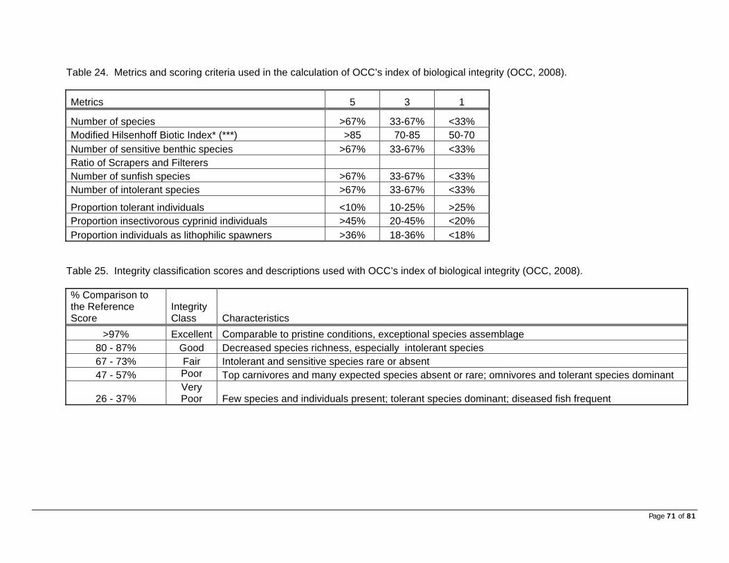
Page 71 of 81
Table 24. Metrics and scoring criteria used i
Metrics
n the calculation of OCC’s index of biolo
5 3
gical integrity (OCC, 2008).
1
Number of species >67% 33-67% <33% Modified Hilsenhoff Biotic Index* (***) >85 70-85 50-70 Number of sensitive benthic species >67% 33-67% <33% Ratio of Scrapers and Filterers Number of sunfish species >67% 33-67% <33% Number of intolerant species >67% 33-67% <33%
Proportion tolerant individuals <10% 10-25% >25% Proportion insectivorous cyprinid individuals > 45% 20-45% <20% Proportion individuals as lithophilic spawner >s 36% 18-36% <18%
Table 25. Integrity classification scores and sed iolo % Comparison to the Reference Score
Integrity Class Character
descriptions u
istics
with OCC’s index of b gical integrity (OCC, 2008).
>97% Excellent Compara ond ecieble to pristine c itions, exceptional sp s assemblage 80 - 87% Good Decrease nes spd species rich s, especially intolerant ecies 67 - 73% Fair Intolerant spe and sensitive cies rare or absent 47 - 57% Poor Top carnivores and many expected species absent or ecie nt rare; omnivores and tolerant sp s domina
26 - 37% Very Poor Few species and individuals present; tolerant species dominant; diseased fish frequent

Page 72 of 81
ssification.
Table 26. Results generated from fish collections made in the study area. Overall ranking determined by combining USAP-IBI support lassification and OCC-IBI integrity clac
SiteName Waterbody IDUSAP-IBI Total
Score
USAP-IBI
ClassificationOCC-IBI Total
ScoreOCC-IBI % of
Reference
OCC-IBI Integrity
ClassificationSite Integrity Classification
Beech Creek OK410210060320G 33 un rmined 2 1.00 excellent unimpairedOK410310020100D 3 u mined 27 0.78 fair inconclusive
Big Eagle Creek OK410210060160L 35 rting 27 0.93 excellent unimpaired_00 3 u ine 25 1.00 excellent unimpaired
OK410310020070C 39 ing 27 0.85 good unimpaired20C 35 ing 27 0.93 excellent unimpaired
420C 3 ing 27 1.00 excellent unimpaired410210060020G 3 ting 27 1.15 excellent unimpaired
0300030020M 3 ting 27 0.93 excellent unimpairedCloudy Creek OK4102 27 1.00 excellent unimpairedCow Creek OK410210060350G 31 u 27 0.85 good inconclusive
OK410210010070G 39 s ting 27 1.00 excellent unimpaired0210090010G 43 s ng 27 1.07 excellent unimpaired
10210080010_00 37 ng 27 1.00 excellent unimpairedGlover River, Upper OK410210080010_00 33 u ined 23 0.85 good inconclusive
r OK410310020010_10 3 rting 23 0.92 excellent unimpairedKiamichi River, Upper OK4103100200 21 0.84 good inconclusiveLittle River OK410210020140_00 39 31 1.15 excellent unimpairedMountain Fork OK410210060010_10 37 23 0.85 good unimpairedOne Creek OK410300030060F 35 supporting 27 1.00 excellent unimpairedRock Creek (McCurtain Co.) OK410200030010G 41 supporting 27 1.15 excellent unimpairedRock Creek (Pushmata Co.) OK410300020190G 35 supporting 27 0.85 good unimpairedTenmile Creek OK410300030270C 31 undetermined 27 0.93 excellent unimpairedTerrapin Creek OK410210020150G 35 supporting 27 0.85 good unimpairedWest Fork of Glover River OK410210080010M 35 supporting 27 1.00 excellent unimpaired
Integrity
dete 7Big Cedar Creek 3 ndeter
suppondetermBilly Creek OK410310020070 3 d
Billy Creek supportBlack Fork of Little River OK4102100300
410300030support
rtBuck Creek OKBuffalo Creek OK
77
supposuppor
Cedar Creek OK41 5 suppor10020300C 33 undetermined
minedndeterupporupp
Cypress CreekEast Fork of Glover River OK41Glover River, Lower OK4
ortisupportindetermsuppoKiamichi River, Lowe 5
10_10 29 undeterminedsupportingsupporting
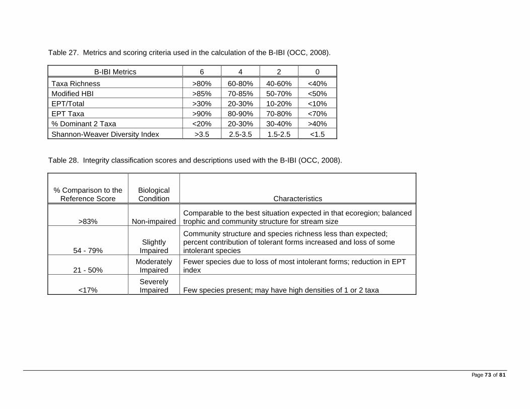
Page 73 of 81
Table 27. Metrics and scoring criteria used in the calculation of the B-IBI (OCC, 2008).
B-IBI Metrics 6 4 2 0 Taxa Richness >80% 60-80% 40-60% <40% Modified HBI >85% 70-85 0-7 50%% 5 0% < EPT/Total >30% 10-20 <10%20-30% % EPT Taxa >90% 80-90 0-8 70%% 7 0% < % Dominant 2 Taxa <20% 20-30% 30-40% >40% Shannon-Weaver Diversity Index >3.5 2.5-3 .5- <1.5 .5 1 2.5
escriptions use he C, 2
% Comparison to the Biological
Table 28. Integrity classification scores and d d with t B-IBI (OC 008).
Reference Score Condition Characteristics
>83% Non-impairedComparable to the best situation expected in that ecoregion; balanced trophic and community structure for stream size
54 - 79% tr
ty structure and species richness less than expected; me Sligh
Impaily ed
percent contribution of tolerant forms increased and loss of sointolerant species
Communi
21 - 50% era
paireduction in EPT Mod tely Fewer species due to loss of most intolerant forms; r
Im ed index
<17% SevImp
erair
ely ed Few species present; may have high densities of 1 or 2 taxa

Page 74 of 81
Table 29. Results generated from macroinvertebrate collections made in the study area. Overall ranking determined by combining results of different sample collections. (* = score is the result of combined collections)
Sitename Waterbody IDSample
TypeIBI Percent of
ReferenceIBI Integrity
ClassificationSite Integrity Classification
Be reek OK410210060320G rif 1.21 NI unimpairedBig Creek OK410310020100D rif 1.08 NI unimpairedBig e Creek OK410210060160L rif 1.05 NI unimpairedBill OK410310020070C rif 1.14 NI unimpairedBla ork of Little River OK410210030020C rif 1.05 NI unimpairedBu eek OK410300030420C rif 1.18 NI unimpairedBu reek OK410210060020G rif 1.08 NI unimpaired
OK410300030020M rif 1.12 NIOK410300030020M veg 1.08 NIOK410300030020M wood 0.91 NIOK410210020300C rif 0.96 NIOK410210020300C veg 1.23 NIOK410210020300C wood 0.82 NI
Co eek OK410210060350G rif 1.06 NI unimpairedCy reek OK410210010070G rif 0.82 NI unimpairedEa rk of Glover River OK410210090010G rif 1.01 NI unimpaired
OK410300010020F rif 1.12 NIOK410300010020F wood 0.85 NIOK410210080010 rif 1.10 NIOK410210080010 veg 0.93 NIOK410210080010 wood 1.36 NIOK410210080010 rif 1.15 NIOK410210080010 veg 1.15 NIOK410310020010 rif 0.69 SIOK410310020010 veg 0.77 SIOK410310020010 wood 1.27 NIOK410310020010 rif 1.15 NIOK410310020010 veg 1.08 NIOK410310020010 wood 1.36 NIOK410210030010 veg 0.77 SIOK410210030010 wood 1.00 NIOK410210020140 rif 1.15 NIOK410210020140 veg 1.08 NIOK410210020140 wood 1.36 NI
Lu OK410210070010G rif 0.98 NI unimpairedOK410210060010 rif 1.15 NIOK410210060010 veg 0.77 SIOK410210060010 wood 1.09 NIOK410210060010 wood 1.09 NIOK410210060010 rif 1.15 NIOK410210060010 veg 0.85 NIOK410300030060F rif 0.93 NIOK410300030060F wood 0.36 MI
Ro (McCurtain Co.) OK410200030010G rif 0.99 NI unimpairedRo (Pushmata Co.) OK410300020190G rif 1.07 NI unimpaired
OK410300030270C rif 0.89 NIOK410300030270C veg 0.92 NIOK410300030270C wood 0.64 SI
Te eek OK410210020150G rif 1.16 NI unimpairedWe of Glover River OK410210080010M rif 1.07 NI unimpaired
Ga reek
unimpaired
unimpaired
unimpaired
Te eek unimpaired
slightly impaired
unimpaired
unimpaired
unimpaired
unimpaired
Mo ork River, Lower
Mo ork River, Upper
On
Glov iver, Lower
Glov iver, Upper
Kia River, Lower
Kia River, Upper
Litt Lower
Lit Upper
Ce reek
Clou reek
unimpaired
unimpaired
slightly impaired
unimpaired
ech C Cedar Eagly Creekck Fck Crffalo C
w Crpress Cst Fo
kfata Creek
ck Creekck Creek
rrapin Crst Fork
tes C
nmile Cr
untain F
untain F
e Creek
er R
er R
michi
michi
le River,
tle River,
dar C
dy C

Page 75 of 81
Table 30. Overall biological ranking generated from collections made in the study area.
Site Name
ish Integr lassifica
n
Macroinvertebrate Integrit
las n
Overall Biological Ranking Waterbody ID
FC
itytio y
C sificatioBeech Creek OK4102 20 pa nim unimpaired 100603 G unim ired u paired Big Cedar Creek OK4103 00 cl nim unimpaired 100201 D incon usive u paired Big Eagle Creek OK4102 60L pa nim unimpaired 100601 unim ired u paired Billy Creek OK4103 70 pa nim unimpaired 100200 C unim ired u paired Black Fork of Little River OK4102 020C pa unimpaired 10030 unim ired unimpaired Buck Creek OK410300030420C unimpaired unimpaired unimpaired Buffalo Creek OK410210060020G unimpaired unimpaired unimpaired Cedar Creek OK410300030020M unimpaired unimpaired unimpaired Cloudy Creek OK410210020300C unimpaired unimpaired unimpaired Cow Creek OK410210060350G inconclusive unimpaired unimpaired Cypress Creek OK410210010070G unimpai unimpaired red unimpaired East Fork of Glover River OK410210090010G unimpaired unimpaired unimpaired Gates Creek OK410300010020F not available unimpaired unimpaired Glover River, Lower OK410210080010 unimpaired unimpaired unimpaired Glover River, Upper OK41 ired 0210080010 inconclusive unimpaired unimpaKiamichi River, Lower K41 ve O 0310020010 unimpaired slightly impaired inconclusiKiamichi River, Upper OK41 inconclusive unimpaired unimpaired 0310020010 Little River, Lower 41OK 0210030010 unimpaired unimpaired unimpaired Little River, Upper OK410210020140 not available unimpaired unimpaired Lukfata Creek K410210070010G not available unimpaired unimpaired OMountain Fork unimpaired OK410210060010 unimpaired unimpaired One Creek OK410300030060F unimpaired slightly impaired inconclusive Rock Creek (McCurtain Co.) OK410200030010G unimpaired unimpaired unimpaired Rock Creek (Pushmata Co.) OK410300020190G unimpaired unimpaired unimpaired Tenmile Creek OK410300030270C unimpaired unimpaired unimpaired Terrapin Creek OK410210020150G unimpaired unimpaired unimpaired West Fork of Glover River OK410210080010M unimpaired unimpaired unimpaired

Page 76 of 81
DISCUSSION AND RECOMMENDATIONS
The Upper Kiamichi, Little, and Mountain Fork River watersheds all have relatively low pH values. everal potential causes include non-point source impacts from silviculture and low mineral
solubility as a result of geology. Silviculture is prevalent throughout the watersheds and each watershed does show elevated turbidity during runoff events. Likewise, low conductivity is characteristic of each watershed and tends to decrease during runoff events. To investigate how each of these causes potentially relate to pH, a series of multiple regression analyses were performed. The three objectives of the analyses were to:
• Determine the best explanatory model for pH using multiple linear regressions (MLR). • Based on the MLR and simple linear regression best fits, determine the most predictive
individual variable for each model. • Based on the MLR and simple linear regression best fits, determine whether conductivity or
turbidity is the best predictor of pH.
Whole dataset models for each test station were relatively consistent. For all three watersheds, the mean daily pH was predicted by stage, discharge, and conductivity. Turbidity was also included as an explanatory variable for the Little River and Mountain Fork River watersheds. For each model, stage was the best predictor as evidenced by higher individual R2 and sequential sum of squares values. The difference in the predictability of conductivity and turbidity is more difficult to ascertain. In the Kiamichi and Little River watersheds, conductivity has superior explanatory power. At the Little River near Cloudy, conductivity is by far a better predictor than turbidity. Model statistics are in favor of conductivity as is the capacity of conductivity as an individual predictor of pH. Turbidity is not an explanatory variable for the Kiamichi River station, which would seem to indicate that conductivity is the superior predictor. However, conductivity is a relatively weak explanatory variable in simple regression models. The picture becomes unclear when considering the Mountain Fork watershed. At the Smithville station, conductivity and turbidity appear indistinguishable as predictors. They demonstrate a fair ability as predictive variables in simple regression models and have similar statistical outputs in the regression model. The whole dataset models for the control watershed models (Billy Creek and Glover River) produced results that were somewhat variable when compared to each other and to test watersheds. Both models have poor predictive capabilities and both show some issues with fit, especially the Glover River station. The Glover River near Glover model is similar in that stage is the best predictor. When considering the weight of evidence including regression coefficients and simple regression R2 values, conductivity is the best predictor of pH at Billy Creek near Muse. Like the Smithville station, conductivity and turbidity appear indistinguishable as predictors at the Glover station. Finally, Billy Creek is the only station that does not use stage as a predictor, which may be a result of its small size in relation to other stations. When considering “runoff” subset models, the results demonstrate that conductivity is the better predictor at most stations. At study test stations, conductivity is the better predictor at both Little River near Cloudy and Mountain Fork River near Smithville, while turbidity is a slightly better predictor at the Kiamichi River near Big Cedar. For both control stations conductivity appears to have good predictive ability. Turbidity has equivalent ability at the Glover River near Glover station, but is an extremely poor predictor at Billy Creek near Muse. However, of all five models, Cloudy is the only station whose subset model is comparable to the whole dataset model. All “runoff” subset models demonstrated very poor fit.
S

Page 77 of 81
When results of both test and control watersheds are considered as a whole, the following conclusions can be made. Runoff, conductivity, and turbidity all have some capacity to explain variation in pH, and as might be expected, fluctuations in stage and/or discharge most affect the variation in pH. The primary question then becomes—what is the comparable effect of conductivity and turbidity on pH variability? Assuming that both variables are highly correlated to runoff, a noticeable lack of multi-collinearity is present in all models suggesting that their explanatory capacity is independent. When simply comparing the predictive power of the two variables at test stations, conductivity has more universal explanatory capacity. Results of control watershed analyses support this conclusion. Even though it is considered the no-impact control, Billy Creek near Muse hacommtest variacontrol (Glover River near Glover), conductivity and turbidity are nearly interchangeable as predictors. However, both are also poor individual predictors in whole dataset models. So, is low regio turbidity a result of a natural or unnatural condition? Weight of evidence would lead to the conclusion that naturally low capacity for mineralization is the primary cause of low pH values.
e , idity does have some explanatory capacity both unimpac and impacted e d
oooe ent in region. Of the 28 com ehens sit oas ss onducted, 93% were s unp o
s g a decision matrix outlined in Table , it must be decided if low pH is naturally occurring and if the ogical ogical ple iss pow located throughout the watersheds. Additionally, the analysis is based on multiple emblaulting fromes are inductivity explained the majority of variance in pH. Based on land use, both parameters should e no anthropogenic influence present in the watershed. Conversely, turbidity, which for this y was considered to be an indicator of non-point source pollution, does have so lanatory
acity. However, it is g rally has much les edictive ability than conductiv ole data lyses, in “runoff” set analyses, dem strated e ss explanatory ity. The clusion uld be that l pH is a naturally o rri in the watersh
g-term na t s eg sh b lo iverporat
nagementsider the ondary question that should influence the impairment decision is what are the consequences? If decision is
s coggids.H is
mng F m
paris nurtost
ablot
herly c
e cpremoon
hemsenre,trol
ict in
coled
al c th
ndu by
hae wcti
na
racate
vitytura
terirs exlly
stichedpla
low
s t, tuins m
o thrbi thine
e tditye mral
est vao
izat
walue
st vion
ters aari. C
shere ancon
dsstile ve
. Dl rein rse
espprepH,ly,
itesen inat t
thetat
diche
faiveatinimp
ct t of g tac
hat the hat ted
ercial lowatershebility in p
nal
ver turbrshe s.
re makingical analved oxyg
Howwat Befbioldissto bconincocom Conthebiolbiolsamaddandassresvaluconhavstudcapanacon Lonincomaconsecthe
in
imgs ll b
ted
ussd ton
g rlysen
ecoes. thr
mm Doug
enespho
daiteut
tion a
the
s pre
stu
abovady
ut lenwa
pHce ters
coof he
ntr303ds,
ols(d
the
, it) lis ov
istinera
poforiolo
rtan bogic
t tth al c
o dpHon
isc anditi
thurbwas
e idit de
resy ater
ultss wmin
of ell ed
excellidered clusive. osite c
iderin
thepai fis
tion
f the
pricalsselig
re
ive itioas pa
dy
e bihi
pair.
ter
sehe , a
ds
mener onl
pai
ts c7%y tw
red
nim Nollec
ll o
redh s w
ab
forcollere
ov
ovect a
e in
erionsse
fo
all s wsse
rma
bioered a
tio
log as s
n, a
cosshtly
the
nded im
stu
n, wimired
wa
le ted
she
othnd
im
eao
for
rnma
pH
ed cro
?
a rinv
Acc
ankert
or
ingebr
ding
of ate
to 31beatrity
re a
ishxhra
comcon imper to
ges
muditioaire th
and na pa
nitn td
e re
uturart
y ishroandsu
singl co
a r
suug a lts.
wnd
esu
pphouvas Th
ell itiolt
ortit tht mer
estns.
of n
ng e wajo
e a
abl Eatu
foreers is nu
ed auslly
a he unmb
indtiveocc
recds iimer
ice reurr
oms opai of
s. Tgreing
mef hiredsta
hess co
ndgh . Ftion
onionnd
atiointeurts o
ly c anitio
n fgri
herve
onalysns.
or ty. mor a
sidis
Fo
act Rere,wid
eraindr a
ionsu thee r
tioispll
calts b
ang
n isutastu
n bindioloe
wblydy
e micatgicof w
het shsta
ade thal sat
herowstion
e. attud
erb
or ths,
C noy
ody
noat low sta
lea sindes siz
t pH
ge
rly, gle ign es
is pH or
meity i ca
ed.
n tes
t th. T
y, th
expn whpac
o th reat ohe
e r
enesubow
trat a dr ef
tat
s pron
ccu
eveitiznc
ty
ed o
and wo
maed i
venditi
ith klaod qu
ly i
leon
conhomdaalit
nflu
ng
peds ond
wa
the
con
wf O goter
like
geme isior-a
de
enOCWns
rch
for
ies shan bt o
of im
ould bouhe
ire
e de cscietire
as
sida.
ta, y m
en
era Tandan
ce
tiohes suage
of t
n ge ggm
urb
e quiutref
eg
valure tcomore
ulat
es hat es , a
ory
n th decove
ma
P being
a s
nd ivefec
us
redy sn t
pa
y thnd en
d b
ene aof
n
valuesent
idit

Page 78 of 81
structure determines that a TMDL will be developed to control turbidity and thereby increase pH. of resources and potential effects on various groups in the
watershed. If the decision is made for a status of unimpaired based on the weight of evidence, the
y watersheds. However, a floor should e established for pH in the region and promulgated as a numerical criterion into the OWQS or
le
the study
s (OGS, 2002). Secondly, low pH values crease the probability of higher levels dissolved constituents. Analysis indicates that low pH is
Consequences include allocation
most obvious consequence is a potential deleterious impact on the biological community. The consequences of the latter seem less likely to happen based on the current status of biological community. The consequences of the former are a given based on regulatory requirements. So, what are the possible outcomes? First of all, low pH is like the result of naturally occurring conditions. For the fish and wildlife propagation beneficial use, consideration should be given to removing low pH (< 6.5) as an impairment cause in the studbwritten as a narrative criterion in the USAP. Because it is based on sound science and defensibdata and considers the potential consequences of action, this should be the most effective long-term management strategy for these watersheds. Secondly, several sites listed for pH inwatersheds are co-listed for turbidity. If turbidity is a possible contributing factor to future ecological health, it should be regulated independent of pH in the TMDL process.
An analysis of metals listings in the study watersheds produced mixed results. The Little River is not impaired for silver based on a comparison of dissolved silver data to the corresponding criterion. At all BUMP stations, the fish and wildlife propagation beneficial use is impaired based on an exceedance of chronic criteria for dissolved lead. The Kiamichi is also impaired based on an exceedance of the acute criterion for dissolved lead. Based on these results as well as the supporting results of the biological studies, a water effects ratio study for lead may need to be conducted in the study watersheds (Table 32). Furthermore, the Little River should not be listed as impaired for copper. However, before further regulatory or management decisions are made for metals in these watersheds, the plausibility that metals are naturally occurring should be considered. Primarily, analytical results and dissolved criteria for both lead and silver are near or below sub-part per billion concentrations. Because lead is naturally occurring in small amounts throughout the watersheds, concentrations could represent natural background levelinnaturally occurring throughout the watersheds. If the recommendations of this report are accepted, a regionally specific pH criterion will be developed or no listings for pH will be made in future 303(d) iterations. Lastly, biological condition throughout the watershed is generally unimpaired. Although independent applicability is the governing principle when considering different types of water quality data for assessment, biological condition should not be ignored when making future regulatory or management decisions for the watershed.

Page 79 of 81
Table 31. Assessment decision matrix used for pH according to application of USAP.
pH
Condition of Biological Community 303(d) Status
Impairment Cause TMDL Status
Supporting Supporting Not Impaired N/A Unnecessary
Supporting Not Supporting Impaired unknown look for other causes
Not Supporting Supporting Impaired low pH naturally occurring
Site or regionally specific criterion set at natural condition
Not Supporting Supporting Impaired
low pH not naturally occurring TMDL
Not Supporting Not Supporting Impaired
low pH naturally occurring
UAA to modify beneficial uSite or regionally specific criterion set at natural cond
se;
ition
Not Supporting Supporting Impaired occurring TMDL Not
low pH not naturally
Table 32. Assessment decision matrix used for metals according to application of USAP.
Metals Concentration
Condition of Biological Community 303(d) Status
Impairment Cause TMDL Status
Supporting Supporting Not Impaired N/A Unnecessary
Supporting Not Supporting Impaired unknown look for other causes
Not Supporting Supporting Impaired metals naturally occurring
Site specific criteria, WER,variance
Not Supporting Supporting Impaired
metals not naturally occurring TMDL
Not Supporting Not Supporting Impaired
metals naturally occurring
UAA to modify beneficial uSite specific criteria set atnatural condition
se;
Not Supporting Supporting Impaired occurring TMDL Not
metals not naturally

Page 80 of 81
REFERENCES
Helsel, D.R. and Hirsch, R.M. 1995. Statistical Methods in Water Resources. 443pp. Kloxin, Greg. Personal Communication. 2008. Minitab, Inc. 2007. Minitab, Release 15 for Windows. Multi-Resolution Land Characteristics Consortium. 2001. National Land Cover Database. URL: http://www.mrlc.gov/ National Atmospheric Deposition Program (NRSP-3). 2009. NADP Program Office, Illinois State Water Survey, 2204 Griffith Dr., Champaign, IL 61820. Oklahoma Conservation Commission. 2005. Analysis of Oklahoma Conservation Commission Physiochemical and Biological Data Toward Determination of High Quality Sites”. Oklahoma City, OK. Oklahoma Conservation Commission. 2008. Small Watershed Rotating Basin Monitoring Program Year 5: Lower Red Basin. Oklahoma City, OK. Oklahoma Department of Environmental Quality. 2006a. Continuing Planning Process. Oklahoma City, OK. Oklahoma Department of Environmental Quality. 2006b. The State of Oklahoma 2006 Water Quality Assessment Integrated Report. Oklahoma City, OK. Oklahoma Department of Environmental Quality. 2007. Quality Management Plan. QMP Track No. 00-182. Oklahoma City, OK. Oklahoma Department of Environmental Quality. 2008. The State of Oklahoma 2008 Water Quality Assessment Integrated Report. Oklahoma City, OK. Oklahoma Geological Survey. 1983. Hydrologic Atlas 9. Norman, Ok. Oklahoma Geological Survey. 2002. Metallic-Mineral Resources of Oklahoma. OGS Special
ublication 2002-1. Norman, Ok. Oklahoma Water Resources Board. 1999. Technical Report 99-3: Standard Operating Procedures for Stream Assessments and Biological Collections Related to Biological Criteria and Development. Oklahoma City, OK. Oklahoma Water Resources Board. 2004. Standard Operating Procedure for the Collection of Fish in Streams. Oklahoma City, OK. Oklahoma Water Resources Board. 2004a. Standard Operating Procedure for the Installation of Nonrecording Gages and Measurement of Stage in Streams. Oklahoma City, OK.
P

Page 81 of 81
rement of Stream Discharge. Oklahoma City, OK. Oklahoma Water Resources Board. 2005b. Standard Operating Procedure for the Recording of Physical/Chemical using a Remotely Deployed Continuously Recording Multiparameter Instrument in Strea a C Oklahoma Water Resources Board. 2006a. of M brates Ok ty, OK Oklahoma Water Resources Board. 2006b. Stand ceWater Quality Sam ms. a City Oklahoma Water Resources Board. 2007. Oklah Quality S ds. OAC 785:45. O K Oklahoma Water Resource Board. 2008a. Implemen a’sC c Use Asse tocols (UOklahoma City, OK. Oklahoma Water Resources Board. 2008b. Okl neficial nitoring Program
ssessment and Watershed Protection Division, Washington, D. C.
Woods, A.J., Omernik, J.M., Butler, D.R., Ford, J.G., Henley, J.E., Hoagland, B.W., Arndt, D.S., and M .C. 2005. s of Oklahoma (color poster with map, descriptive text, summary tables, and photographs): Reston, Virginia, U.S. Geological Survey (map scale 1:1,250,000).
Oklahoma Water Resources Board. 2005a. Standard Operating Procedure for the Measu
Parametersms. Oklahom ity, OK.
Standard Operating Procedure for the Collection acroinverte in Streams. lahoma Ci .
ard Operating Pro, OK.
dure for the Collection of ples in Strea Oklahom
oma Water tandarklahoma City, O .
tation of Oklahomssment Pro
Water Quality Standards, SAP). OAC 785:46-15. hapter 46, Sub hapter 15: Support
ahoma’s Be Use MoA
nnual Report. Oklahoma City, OK.
Plafkin, J. L., M. T. Barbour, K. D. Porter, S. K. Gross, R. M. Hughes. 1989. Rapid Bioassessment Protocols for Use in Streams and Rivers. USEPA/444/4-89-001. U. S. E.P.A, A
oran, B Ecoregion