money, fdi and economic growth in mena countries
TRANSCRIPT

University of New Orleans University of New Orleans
ScholarWorks@UNO ScholarWorks@UNO
University of New Orleans Theses and Dissertations Dissertations and Theses
Spring 5-22-2020
Money, FDI and Economic Growth in MENA Countries. Money, FDI and Economic Growth in MENA Countries.
Huda Alsayed University of New Orleans, [email protected]
Follow this and additional works at: https://scholarworks.uno.edu/td
Recommended Citation Recommended Citation Alsayed, Huda, "Money, FDI and Economic Growth in MENA Countries." (2020). University of New Orleans Theses and Dissertations. 2716. https://scholarworks.uno.edu/td/2716
This Dissertation-Restricted is protected by copyright and/or related rights. It has been brought to you by ScholarWorks@UNO with permission from the rights-holder(s). You are free to use this Dissertation-Restricted in any way that is permitted by the copyright and related rights legislation that applies to your use. For other uses you need to obtain permission from the rights-holder(s) directly, unless additional rights are indicated by a Creative Commons license in the record and/or on the work itself. This Dissertation-Restricted has been accepted for inclusion in University of New Orleans Theses and Dissertations by an authorized administrator of ScholarWorks@UNO. For more information, please contact [email protected].

Money, FDI and Economic Growth in MENA Countries
A Dissertation
Submitted to the Graduate Faculty of the
University of New Orleans
in partial fulfillment of the
requirements for the degree of
Doctor of Philosophy
in
Financial Economics
by
Huda Alsayed
B.S. King Abdelaziz University, 2009
M.S University of New Orleans, 2014
M.S University of New Orleans, 2017
May, 2020

ii
Table of Contents
LIST OF FIGURES: ................................................................................................................ iii
LIST OF TABLES: .................................................................................................................. iv
Abstract: .................................................................................................................................... v
Chapter 1: .................................................................................................................................. 1
FDI, Trade Openness, Capital Formation, and Economic growth in MENA countries
analysis. And whether FDI is a complement or substitute for stock market development
in MENA countries. .................................................................................................................. 1
1.Introduction: .......................................................................................................................... 1
2. Literature review: ................................................................................................................. 6
3. Data and Methodology: ...................................................................................................... 11
4. Empirical Result: ................................................................................................................ 15
5. Summary and Conclusion: ................................................................................................. 24
Chapter 2: ................................................................................................................................ 27
Money demand function and its Stability in MENA countries. ......................................... 27
1.Introduction: ........................................................................................................................ 27
2.Literature review: ................................................................................................................ 28
3. Data and methodology:....................................................................................................... 31
4.Empirical Result: ................................................................................................................. 33
5. Summary and conclusion: .................................................................................................. 43
References:............................................................................................................................... 45
Appendix:................................................................................................................................. 52
chapter 1: ............................................................................................................................... 52
a) Variable explanation and sources: .................................................................................... 52
Chapter 2: .............................................................................................................................. 54
a) Variable explanation and sources: ................................................................................ 54
B) Explanation of variables on demand for money .............................................................. 55
VITA......................................................................................................................................... 58
iii
LIST OF FIGURES:
Chapter 1
FIGURE 1-REPRESENT THE PERCENTAGE OF TRADE AND FDI INFLOW FOR MENA
COUNTRIES. ......................................................................................................................... 5
FIGURE 2- REPRESENT THE PERCENTAGE OF STOCK AND FDI INFLOW FOR MENA
COUNTRIES. ......................................................................................................................... 6
Chapter 2
FIGURE 3- REPRESENT THE STABILITY OF THE MONEY DEMAND GRAPH:
(BAHRAIN, KSA, KUWAIT, QATAR, UAE, OMAN, JOURDAN, ALGERIA, EGYPT,
IRAN, IRAQ, LEBANON, LIBYA, TUNISIA, MOROCCO) RESPECTIVELY: ............. 42

iv
LIST OF TABLES:
Chapter 1:
TABLE 1-SUMMARY OF THE EMPIRICAL STUDY ON STOCK MARKET
DEVELOPMENT: ................................................................................................................ 10
CONTINUE TABLE 1-SUMMARY OF THE EMPIRICAL STUDY ON STOCK MARKET
DEVELOPMENT: ................................................................................................................ 11
TABLE 2-VARIABLES USED, THEORY INTUITION AND PRIORI EXPECTATION: ...... 13
CONTINUE TABLE 2-VARIABLES USED, THEORY INTUITION AND PRIORI
EXPECTATION: .................................................................................................................. 14
TABLE 3-THE PAIRWISE CORRELATION FOR GROWTH, FDI, TRADE, LABOR, AND
CAPITAL FORMATION: .................................................................................................... 15
CONTINUE TABLE 3-THE PAIRWISE CORRELATION FOR GROWTH, FDI, TRADE,
LABOR, AND CAPITAL FORMATION:........................................................................... 16
TABLE 4-PAIRWISE CORRELATION WITH FDI AND STOCK: ......................................... 16
TABLE 5-UNIT ROOT STATIONARY TEST FOR LM PESARAN AND FISHER (ADF). ... 17
TABLE 6-COINTEGRATION TEST FOR PEDRONI AND KAO:........................................... 18
TABLE 7-POOLED OLS AND FIXED EFFECT GROWTH FOR LONG RUN RELATION: 19
TABLE 8-VARIANCE INFLATION FACTOR: ........................................................................ 20
TABLE 9-POOLED OLS AND FIXED EFFECT GROWTH FOR LONG-RUN RELATION
AND EDUCATION: ............................................................................................................ 21
TABLE 10-POOLE OLS AND A FIXED EFFECT FOR STOCK MARKET DEVELOPMENT
AND FDI: ............................................................................................................................. 23
TABLE 11-THE VARIANCE INFLATION FACTOR FOR STOCK AND FDI: ...................... 24
TABLE 12-SUMMARY STATISTICS: ...................................................................................... 34
TABLE 13-PAIRWISE CORRELATION: .................................................................................. 34
TABLE 14-POOLED OLS AND FIXED EFFECT OF LONG-RUN RELATION FOR THE
DEMAND FOR MONEY: ................................................................................................... 35
TABLE 15-VARIANCE INFLATION FACTOR: ...................................................................... 36
TABLE 16-UNIT ROOT TEST STATIONARY: ........................................................................ 37
TABLE 17-PEDRONI AND KAO COINTEGRATION TEST: ................................................. 37
TABLE 18-ARDL MODEL SHORT-RUN VS LONG-RUN RELATIONSHIP:....................... 38
CONTINUE TABLE 18-ARDL MODEL SHORT-RUN VS LONG-RUN RELATIONSHIP: . 39
CONTINUE- TABLE 18-ARDL MODEL SHORT-RUN VS LONG-RUN RELATIONSHIP: 40

v
Abstract:
The first chapter examines the link between FDI, trade, capital formation and economic
growth in 12 MENA countries using panel analysis for yearly data between the period 2001 to
2017. Using the cointegration and Hausman test, our results indicate that, all the variables are
stationary at first level, and the long-run relationship exists between our variables. A model of
endogenous growth highlights that MENA countries favored FDI to trade, where trade has a
negative relationship with economic growth. Capital formation and labor have a positive and
significant relationship. We also, address the relation of education level, as we know that increase
in Education level will enhance the adoption of foreign technology. The results were consistent
with our initial model. Furthermore, we answered the question of whether FDI is a compliment or
a substitute? Our results show that FDI has a negative relation with the stock market. In other
words, FDI is a substitute not a compliment to the stock market. FDI is positively correlated with
political stability, stock market, liquidity, saving, and GDP.
The second chapter explores the long-run demand for money and its stability for MENA
countries for the period of 2002 to 2016 using annual data. By applying a panel cointegration
approach, the result reveals evidence of cointegration between the variables in the long run.
Therefore, an error correction (ECM) is applied to determine the factors that influence real money
aggregate(M2). The result shows that export and import have positive and negative effect
respectively, an increase in exporting will increase the value of the currency, and the opposite is
true. Further, all the variables have a significant effect in the long run, while GDP affects the
demand for money in the short run. The CUSUM test of paraments stability shows that the money
demand function is mostly stable over the period. At the individual level, the results change from
one county to another.
Keywords:
Money demand, exchange rate, Export, Import, FDI, Stock, Trade, Economic growth, Capital
formation MENA Countries.

1
Chapter 1:
FDI, Trade Openness, Capital Formation, and Economic growth in MENA countries analysis. And whether FDI is a complement or substitute for stock market development in MENA countries.
1.Introduction:
Economic literature discusses excessively the relation between foreign direct investment
(FDI) and economic growth in less developed countries. There is a long debate on how FDI, affects
the host country, economist believes that FDI increases the growth of a country in many different
channels. It helps increase employment, creates jobs, and motivate technological changes by
introducing new technology. This technology will generate positive spillovers for local firms. As
technology develops in the host country, FDI is expected to improve the knowledge through labor
training, skill acquisition and flow. FDI also, introduces new management practices and a more
efficient organization of the production process. Therefore, FDI improves the productivity of host
countries not only at the firm level but on the economy of the host country and motivates its
economic growth. Pugel (2007) finds FDI increases technological spillover, promotes the
competition in the industry, and improves the productivity of goods and services for the host
country and therefore increases their economic growth.
On the other hand, some studies that disagree with the statement that FDI has a positive
impact on the host country. Hanson (2001) and Gorg and Greenaway (2004) argue that FDI does
not create positive spillover to the host country. Blomstrom and Kokko (2003) argue that it may
take time for the host country to adjust to the new technology and that the local condition is an
important influence for the host country.
International trade also, has a role in developing the economic growth of a country through the
adoption of superior production technology and innovation. Belloumi (2014) study the
relationship between the trade, FDI in economic growth and he finds that trade openness and
economic growth endorse the long-run relation of FDI, and it serves as a broadcast belt to transfer
technical knowledge. Therefore, trade openness has a positive impact on economic growth.
From that argument we can say that both FDI and trad play a major role in improving
economic growth in countries, however, this effect may vary from country to another. Human
capital also, plays their roles in observing capacity in the host country. Further, Capital formation

2
is used to fund the development programmer in the country, they use it to build schools’ hospitals,
roads, and its play major roles in decreasing poverty, and improve economic development.
Therefore, the link between FDI, Trade Openness, capital formation, and economic growth tends
to be positive.
Capital formation increases the economic growth how? When the government increases
the injection of capital in the form of long-term investments, productivity will increase and
influence economic growth. The growth theory assumes that increase the efficiency of investment
brought by FDI provides comparative advantages, where the local company will compete to catch
up and therefore increase the economy in the long run (Romer 1986). Further, macroeconomic and
political stability may play a role in FDI and trade effect. The literature supports the fact that less
developed countries face a high inflation rate, and macroeconomic instability is not in favor of
economic growth.
There is 2 theory for economic growth, first the neoclassical model, which only show the
impact of technology on economic growth, this model is not able to identify the determinant of
technological progress. The other theory is the growth theory which established to know the
determinant that impacts technological progress. It focuses on what drives growth like innovation,
creation. The difference between both of them is that, neoclassical assumes the technological
progress to be exogenous while growth theory assumes that technology is a form of investment
spill over as endogenous. The implication of technology been endogenous is that economic growth
may be slowing down because of favor, and/ or protecting the existing industry. Theories present
different sources of technological spillover like FDI, human capital, science, all these assume
endogenous technological is the main driver of economic growth in the long run. The finding of
both theories may differ, Mello and Luiz (1999) study the FDI in time series and panel data, they
find that neoclassical model when FDI is exogenous can only affect growth in the short run,
because of the diminishing return in the long run, while the new growth theory when technology
(FDI) is endogenous can find the long-run effect on growth because the knowledge that occurs
with FDI transfer, and continue for a long term, therefore the return will harvest in the long-run.
Counting FDI as endogenous in the model will result in the long-run effect of FDI.
Shahbaz and Rahman (2010); stress out that FDI inflows boost stock market competition,
where there is a high chance that FDI inflows end up listing their shares on the stock market of the
host country. In other words, FDI can enhance the liquidity of the stock markets if foreign investors

3
were able to obtain shares in the host country. Nguyen & Hanh (2012) investigate the stock market
development determinant of Southeast Asian Countries and find that Stability, liquidity, savings,
financial development, and growth affect the stock market positively, while inflation has a negative
effect. Dev & Shakeel (2013), look at the stock market development determinant in Pakistan and
they find that liquidity and investment are the determinate that affect the stock market
development. Ayunku & Etale (2013), study Nigeria’s stock market development and find that
inflation and saving affect the stock market negatively, while the exchange rate market
capitalization and banking has a positive influence on the stock market. Acquah- Sam (2016) look
at Ghana stock market determinant and find that Growth and capital formation affect the stock
market development positively while treasury bill affects it negatively. FDI and Inflation do not
affect the stock market. Islam et al. (2017) study the stock market development in Bangladesh and
he finds that inflation, growth, and market capitalization are the major influence on the stock
market.
Kaehler et al. (2014), investigate the Iraq stock market and he finds inflation, electricity,
political stability, interest rate, and exchange rate, has an impact on the development of their stock
market. Yusoff & Guima (2015) study the determinant of the stock market in 3 countries Saudi
Arabia, Tunis, and Egypt they find that Growth, Savings, Interest rate, Exchange rate, inflation,
and oil rent have a significant impact on stock market development.
As we have seen there is no strict rule whether FDI will affect less developed countries
positively or negatively. Thus, the studies contribute to the existing literature by, uniform a model
that studies the relation between FDI, trade, labor, capital formation, inflation-CPI
(macroeconomic stability), political stability and its effect on economic growth. Furthermore, we
investigate the role of FDI on the stock market development of the host country and whether it is
complements or substitutes. Our interest falls for MENA country which we use 12 countries from
2001 to 2017. In the stock market we had to drop our sample to 10 countries because of the lack
of stock data for Iraq and Algeria. We restrict our sample for this period because of the availability
of the data. Our contribution in this paper is to provide a link between FDI, Trade, Capital
formation, and economic growth. Also, we address the effect of education level on FDI, Trade,
Capital formation, and economic growth to see if it would change our result. Further, we ask the
question of whether FDI is a substitute or a complement to stock market development? As far as
we know we are the first paper to address this issue in MENA reason. In our analysis, we divide

4
our study into two sections, first we study the long-run relation using a panel for all the country.
Our major result indicates that a long-run relationship exists between economic growth
determinant consistent with Mello and Luiz (1999). In pooled OLS our FDI and trade are
complementing to each other however this change after taking the Fixed effect where trade has
negative relation, that could be due to change in the regulation or quote of the tariff. Another reason
is the decline in oil prices in the Middle East could affect where there is a positive relationship
between oil prices and trade. Political stability does not affect our model, while inflation-CPI has
a negative relation with growth in the Fixed effect, which indicates that the government needs to
increase the effort to make all the essential income adjustments for people to retain a good quality
of life. Our labor force and capital formation are positive and significant an increase in economic
growth will increase the capital formation (government support) and labor. We also, add a section
where we include the education level (primary and secondary level) and its proxy for human capital
according to Berthelemy and Demurger (2000). And the results were consistent with our initial
result. We find a negative relation between the secondary education level and the growth, that
could be due to less graduated human capital from the secondary level.
Next we look at the effect of FDI on the stock market development. So, we take the stock
market determinate and see its relationship with FDI. Our result indicates, FDI and the stock
market development do not complement, however, they are substitute, and that liquidity and saving
have a positive relationship with FDI. The more the stock market is liquid the more the investors
can access their savings and therefore invest in FDI. Also, the higher the saving the more inflow
of capital that can be used in investing in FDI. Further, the more stable the exchange rate the less
is currency risk, and therefore attract more FDI. Lastly, GDP and political stability have a positive
relationship with FDI. An increase in the level of income will increase the attraction of FDI, and
the more the country is stable the more the inflow of FDI.

5
Figure 1-Represent the percentage of trade and FDI inflow for MENA countries.
As we can see from the graphs KSA has the most inflow of FDI for that period. One reason
is that during the Arab spring the follow of FDI dropped sharply for some Arab countries like
Tunisia, however, Some GCC counties benefit from that like Saudi Arabia where the flow of FDI
increased. Following KSA comes UAE, then Egypt is the hired country that has a high inflow of
FDI then Iran, and Lebanon then the rest of the courtiers. Looking at the trade graph we can see
that UAE and Bahrain they trade more than other countries, KSA surprisingly is less than them in
the trade that could be due to the oil price drop that happened in the late 2014 begging of 2015
where the oil price drop to almost half from 100S to 50S. Other countries Jorden, Oman Iraq, Tunis
they trade more than they have FDI inflow. Algeria, Morocco, Lebanon we can see it’s almost
equal the inflow of FDI and Trade.

6
Figure 2- Represent the percentage of stock and FDI inflow for MENA countries.
Stock FDI Inflow
The graphs show that KSA has the most flow of FDI for that period followed by the UAE,
Egypt is the hired country that his high percentage of inflow of FDI then Iran, and Lebanon then
the rest of the courtiers. Looking at the Stock market development we can see that Jorden, KSA,
and Bahrain have the highest percentage of the stock market.
The remainder of the paper is organized as follows, section 2 literature review. Section 3
methodology and data, section 4 result. Section 5 conclusion.
2. Literature review:
I. Empirical researches, that study FDI led growth hypothesis (FLGH), find that FDI will
have a positive impact on the host country by providing new technologies, skills, creating
new jobs, increase domestic opportunities, challenges, and expanding access to worldwide
marketing networks. According to Wang and Blomstrom et al. (1992), study FDI and its
effect on the host country, his results show that developed countries benefit more from FDI
that non-developed countries. Borensztein et al (1998) study FDI and its effect on
economic growth, he finds that the effectiveness of FDI depends on the human capital in
the host country, regardless of what positive spill will FDI have on the host country.
Another study by Carkovic and Levine (2002) indicates that years of school do not have a
critical effect on FDI with economic growth. Darrat et al. (2005) analyze the impact of
FDI on economic growth in Central and Eastern Europe (CEE) and the Middle East and

7
North Africa (MENA) regions. They find that FDI affects economic growth in EU
countries, while there is no impact or even negative impact of FDI on economic growth in
MENA and non-EU. Hisarciklilar et al. (2006) study the impact of FDI in some less
developed countries and he finds no causality relation between FDI and GDP for most
Mediterranean countries (Algeria, Cyprus, Egypt, Israel, Jordan, Syria, Morocco, Turkey,
and Tunisia for the duration between 1979-2000). Alia and Dcal (2003), study the effect of
export-led growth hypothesis (ELGH) and FDI led growth hypothesis (FLGH) in turkey,
they find a positive spillover from ELGH, but no spillover effects from FDI to GDP.
Rahman (2007) study the impact of export FDI on real GDP for Asian countries
(Bangladesh, India, Pakistan and Sri Lanka) using the bounds testing approach (ARDL)
technique for cointegration for the period of 1976-2006. The result confirms the
cointegrating relationship between variables in all countries. Overall, they find that FDI
always affects real GDP. Jallab, Gbakou, and Sandretto (2008) study the relation in MENA
countries, they use a dynamic panel procedure for the period of 1970- 2005. For their
testing they use GMM and 2SLS estimators, they find that there is no independent impact
of FDI on economic growth, and the growth-effect of FDI does not depend on trade
openness and income per capita. On the other hand, macroeconomic stability played a huge
role in the positive effect of FDI on economic growth. Hassan, Sanchez, and Suk Yu (2011)
study the role of financial development (accounting) on economic growth. Their result
shows that there is a positives relationship between financial development and economic
growth in OIC developing countries. Adhikary (2011) study the relation between Labor,
FDI, Capital Formation, Trade, and economic growth in Bangladesh for the period between
1986 to 2008. He finds a negative relation with trade and it decreases economic growth.
Belloumi (2014) examines the causal relationship between, economic growth, FDI, trade,
labor, and capital investment in Tunis for the period 1970-2008. The author uses the ARDL
model of cointegration to investigate the long-run relationship, the result reveals that
variables are cointegrated when FDI is the dependent variable. Trade openness and
economic growth promote FDI in the long run. Budiharto, Suyanto, Pratono (2017) study
the relation between FDI, Trade, Labor, Capital Formation, and economic growth in
Indonesia. They use annual Time series data from 1985 to 2015 using Autoregressive
distribution lag ARDL. Their result reveals that labor is an important source to attract FDI

8
and to improve the invention scale for trade activities. Furthermore, FDI reveals to be the
main sponsor for capital formation injection. They also, suggest that Investors and
liberalization should be promoted to open the gate for more new investors in Indonesia,
which is regarding what labor force can adopt from the technological spillover derived
from FDI. Safitri (2014) Study the effect of trade, FDI on economic growth and they find
a positive relation with economic growth. The emphasis that countries with more open
trades or less restrictive regulation to the world would increase their economy due to the
accumulation of physical and technological transfer. Further, openness will increase the
capital inflow of the country and therefore, strengthening the economic growth as defined
by endogenous growth theory. Romer (1986) finds that a more open trade economy allows
the country to have comparative advantages and therefore, increase capital accumulation
as it enhances the level of export. Lucas, (1988) finds the trad and FDI have inverse relation
an increase in one may lead to a decrease in the other one. GLevine (2002) argues that
there is no relation between FDI and economic growth, but the relationship between trade
and economic growth may vary. Levine and Carkovic (2002) disagree with the argument
that FDI has a positive growth effect in countries with the developed financial markets
because FDI flow does not have an impact on growth in financially developed countries.
On the other hand, Roland-Holst, Mensbrugghe (2006) find that trad and FDI may be
complementary to one another, like an increase in FDI will result in technological spillover
and increase the export level (trade), as the increase in FDI will increase trade. Yucel
(2009) study the relationship between financial development, trade, and economic growth
in Turki, the result shows that trade has a significant impact on economic growth. Capital
formation is also, one of the determinants that affect economic development, Romer (1990)
indicates that poverty may slow the development of the country because of low income
and therefore low saving, and low investment. However, he also, indicates that the ability
to invest does not depend only on saving but also, on the ability and willingness to invest.
Berthelemy and Demurger (2000), study the relation between FDI and economic growth
in China. They include human capital which is proxy for the education level (primary and
secondary). They indicate that as the share of education level increase the positive effect
of FDI on economic growth will increase. They also, find a positive relation between
Economic growth and FDI.

9
II. Levine and Zervos (1998), and Beck and Levine (2004) emphasize that stock market
development plays an important role in predicting future economic growth. So, we study
the relation between FDI and stock market development, and try to answer the question of
whether FDI a complement or substitute for the stock market? Hausmann and Fernandez-
Arias (2000) study the relationship between FDI and the stock market development in Latin
America, and they analyze whether FDI is good or bad cholesterol? they conclude that FDI
is nothing more than a substitute to the stock market, and that bad effect of FDI comes
from exchange rate expectation and interest rate for the short run. Further, they observe
that countries who are riskier, more distant, financially underdeveloped and institutionally
weaker have a higher inflow of FDI. In light of their statement we can say that FDI
correlates negatively with the development of stock markets. Stijn Claessens, Daniela
Klingebiel, and Sergio L. Schmukler (2001) study the relation between FDI and stock
market development in 77 countries. They found FDI is a complement for stock market
development. Jeffus (2004) analyzes the issue of FDI and stock market development in
four Latin American countries. They hypothesize that FDI has a positive relation with stock
market development, they find that there is a positive and significant correlation between
FDI and stock market development. They also, indicate that FDI is a predictor for stock
market development. They also, argue that listing the company in the stock market will
lead to an increase in the capital of the firm, and increase the development of the local stock
market. Ben Naceur et al. (2007) study the macroeconomic determinants of stock market
development in some MENA countries. Using unbalanced panel data from 11 MENA
countries for the period 1979-1999. Applying fixed and random effects specifications, they
found that saving rate, credit to the private sector, the ratio of the value traded to GDP and
inflation change are the important determinants of stock market development. Rhee and
Wang (2009), they study the relation between FDI and stock market development in
Indonesia, for the years of 2002 to 2007. They find a negative correlation between FDI and
Liquidity stock market, and that will affect the future of Stock market development. Sekhri
and Haque (2015), examined the relationship between FDI and stock market development
in India. They find a positive relation between FDI and stock market development. They
conclude that FDI improves the Indian stock market, which is due to the increase in

10
technology application, new skills and experience, which lead to an efficient industry. Ho
and Iyke (2017) investigate the determinants of stock market development by studying the
existing literature. They find that there are two groups that determent the stock market
development these two major groups are; macroeconomic factors and institutional factors.
First the macroeconomic factors, real income has a positive relationship on the stock mark,
while inflation and exchange rate harm stock market development. However, the banking
sector, interest rate, and private capital flow they had a different argument about them some
studies argue that they have a positive relationship while others argue that they have a
negative effect on the development of the domestic stock markets. Looking at institutional
factors, such as protection of investors, governance stability, financial liberalization and
trade openness all have a positive influence on the stock market development.
Table 1-Summary of the empirical study on stock market development:
Author Country Methodology Finding
Kunofiwa
Tsaurai et al
(2018)
22 Emerging markets,
for the period 1994 to
2014.
Applying
Pooled OLS
fixed and
random
effects
approach
They find that FDI, savings, economic
growth, trade openness, exchange rates,
banking sector development and stock market
liquidity had a positive impact on stock
market development in emerging markets.
Ben Naceur et al.
(2007)
Using unbalanced panel
data for 11 MENA
countries for the period
1979-1999.
Applying
fixed and
random
effects
specifications.
They find that saving rate, credit to the private
sector, the ratio of the value traded to GDP
and inflation change are the important
determinants of stock market development.
Cherif and
Gazdar (2010)
Using data for 14
MENA countries from
1990 to 2007
Using both
panel data and
instrumental
variable
techniques
They find that income level, saving rate, stock
market liquidity, and interest rate influence
stock market development. Further, the result
shows that banking and the stock market
sectors are complementary instead of being
substitutes

11
Continue Table 2-Summary of the empirical study on stock market development:
Raza, Iqbal,
Zeshan Ahmed,
Mohammad
Ahmed, and
Tanvir Ahmed
(2012)
Using the Pakistan
region for the period
1988-2009.
Using
Ordinary
Least Square
(OLS)
method.
They use FDI, saving, EX, and inflation. They
find a positive significant impact of FDI, and
domestic savings on Stock market
development in Pakistan. While the exchange
rate has a negative significant impact, and
inflation does not impact stock market
development.
Hausmann and
Fernandez-Arias
(2000)
Using the Latin
America region up to
1999.
using cross-
section
Ordinary
Least Squares.
They use GDP, POS, Privet credit, saving,
distance, Openness. The major finding is that
FDI is nothing more than a substitute for the
stock market.
Yusoff & Guima
(2015)
Using 3 MENA
countries (Egypt, Saudi
Arabia and Tunisia)
from 1992 to 2012.
Using
Correlation
Analysis.
They find that factors such as oil rent, income
per capita, domestic savings, interest rates,
exchange rates and inflation have an impact
on stock market development in the MENA
region.
Acquah- Sam
(2016)
Using Ghana for the
period between 1991 to
2011.
Linear
regression
analysis
He finds that FDI and inflation do not
influence stock market development whereas
treasury bill rates negatively affected stock
market development in Ghana. Economic
growth and gross capital formation affect the
stock market positively and significantly.
Malcus, Persson
(2018)
Using Swedish
quarterly data observed
between 1982 and 2017.
Time-series
regression
analysis
They find No significant relation between
FDI and stock market development and that
FDI is more of a substitute for the stock
market in the short run.
3. Data and Methodology:
Our sample runs from 2001 to 2017 annual basis for MENA countries (Algeria, Bahrain, Egypt,
Iran, Iraq, Jorden, Lebanon, Morocco, Oman, Tunisia, United Arab Emirates (UAE), Kingdom of

12
Saudi Arabia (KSA). We constructed our data from the World Bank database, the following
equation represents our long-run relation.
𝐿𝑛𝑌𝑖𝑡=𝛽0 + 𝛽1𝑖𝐾𝑖𝑡 + 𝛽2𝑖𝐿𝑛𝐿𝑖𝑡 + 𝛽3𝑖𝐿𝑛𝐹𝐷𝐼𝑖𝑡 + 𝛽4𝑖𝑙𝑛𝑇𝑖𝑡 + 𝛽5𝑖𝑙𝑛𝐼𝑁𝐹𝐶𝑃𝐼𝑖𝑡 + 𝛽6𝑖𝑙𝑛𝑃𝑂𝑆𝑖𝑡 + 𝜀𝑖𝑡
(1)
Where the subscript i=1, ......, N denotes the country (in our study, we have 12 countries) and t=1,
......, T denotes the time period (our time frame is 2001–2017). Y is the GDP Per capita, which is
proxy for economic growth, K is the capital formation, and its Average annual growth of gross
fixed capital formation which used as a fund for national development programmer in the country.
L is the labor force, involving people who supply labor for the production of goods and services
during a specified period. Changes in the Labor force is measured by taking the labor/GDP (2018)
Fernando Martin. FDI is net inflow and measured as % GDP. T is trade Openness measured by
the percentage of the total sum of export and import value from GDP. INFCPI is the Inflation
consumer price index used as a proxy for macroeconomic stability. Jallab, Gbakou, Sandretto
(2008) use Inflation as a proxy for macroeconomic stability, they indicate that the positive impact
of FDI on economic growth depends on macroeconomic stability. The impact of inflation is
measured by the annual percentage change in consumer prices. POS is political stability use as a
measure of politically motivated violence and terrorism.
The following section will explore the effect of FDI, on stock market:
𝑙𝑛𝐹𝐷𝐼 =𝛽0 + 𝛽1𝑖𝐿𝑛𝐺𝐷𝑃𝑖𝑡 + 𝛽2𝑖𝐿𝑛𝑆𝑡𝑜𝑐𝑘𝑖𝑡 + 𝛽3𝑖𝐿𝑛𝑃𝑂𝑆𝑖𝑡 + 𝛽4𝑖𝑆𝐴𝑉𝐼𝑁𝐺𝑖𝑡 + 𝛽5𝑖𝑙𝑛𝐼𝑁𝐹𝑖𝑡 +
𝛽6𝑖𝑙𝑛𝐸𝑋𝐶𝐻𝐴𝑁𝐺𝐸𝑖𝑡 + 𝛽7𝑖𝑙𝑛𝑏𝑎𝑛𝑘𝑖𝑡 + 𝛽8𝑖𝑙𝑛𝐿𝑖𝑞𝑢𝑖𝑑𝑖𝑡𝑦𝑖𝑡 + 𝜀𝑖𝑡 .(2)
Where the subscript i=1, ......, N denotes the country (in our study, we have 10 countries) and t=1,
......, T denotes the time period (our time frame is 2001–2017).
Where, Foreign direct investment, Net FDI (% of GDP). POS: political stability an institutional
factor, where an increase in political stability will motivate the FDI to invest in the host country.
Macroeconomic factors: are GDP is the Income level and it’s usually positive and significant with
FDI. Stock market development, Stock market capitalization (% of GDP) expect to have a negative
relation with FDI. Banking sector development, Domestic credit to the private sector by banks (%
of GDP) it measures the role of a bank in providing long term financing to a private corporation.
Gross savings, Gross domestic savings (% of GDP) usually it has a positive relation with FDI.

13
Inflation consumer prices (annual %) rate, supposed to have a negative relation with the stock
market. The stock market liquidity, the Stock market traded value (% of GDP) We expected to
have a positive impact on FDI.
Table 3-Variables used, theory Intuition and Priori Expectation:
Variable Theory intuition source Expected
sign
Capital
formation
Capital formation is important for any country
to become self-sufficient and less dependent of
foreign resources, it increases job opportunities,
make better use of natural resources, gain high-
quality goods, and increase in economic growth
and living standard in the long run for the
people.
Cohen and
Levinthal
(2012);
+
Labor Labor is used as indicators to attract FDI and
increase scales for trade activities.
Budiharto,
Suyanto,
Pratono (2017
+
Trade study the relation between FDI, Trade, Labor,
Capital Formation, and economic growth in
Bangladesh for the period of 1986 to 2008. He
finds a negative relation with trade and it
decreases economic growth. Other papers say
that trade might have a positive relation with
economic growth.
Adhikary
(2011)
+/-
FDI Indicates that FDI increases technological
spillover and brings positive spillover to the
host country and therefore increases their
economic growth. Other paper indicates that
FDI does not have a positive spill to the host
country.
Pugel (2007);
Hanson
(2001)
+/-
Political stability improvement in political risk will positively
affect Economic growth and attract more FDI
inflows into a country.
Cuyvers et al
(2011)
+
14
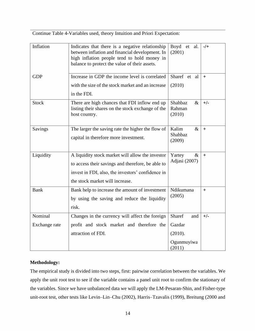
Continue Table 4-Variables used, theory Intuition and Priori Expectation:
Inflation Indicates that there is a negative relationship
between inflation and financial development. In
high inflation people tend to hold money in
balance to protect the value of their assets.
Boyd et al.
(2001)
-/+
GDP Increase in GDP the income level is correlated
with the size of the stock market and an increase
in the FDI.
Sharef et al
(2010)
+
Stock There are high chances that FDI inflow end up
listing their shares on the stock exchange of the
host country.
Shahbaz &
Rahman
(2010)
+/-
Savings The larger the saving rate the higher the flow of
capital in therefore more investment.
Kalim &
Shahbaz
(2009)
+
Liquidity A liquidity stock market will allow the investor
to access their savings and therefore, be able to
invest in FDI, also, the investors’ confidence in
the stock market will increase.
Yartey &
Adjasi (2007)
+
Bank Bank help to increase the amount of investment
by using the saving and reduce the liquidity
risk.
Ndikumana
(2005)
+
Nominal
Exchange rate
Changes in the currency will affect the foreign
profit and stock market and therefore the
attraction of FDI.
Sharef and
Gazdar
(2010).
Ogunmuyiwa
(2011)
+/-
Methodology:
The empirical study is divided into two steps, first: pairwise correlation between the variables. We
apply the unit root test to see if the variable contains a panel unit root to confirm the stationary of
the variables. Since we have unbalanced data we will apply the LM-Pesaran-Shin, and Fisher-type
unit-root test, other tests like Levin–Lin–Chu (2002), Harris–Tzavalis (1999), Breitung (2000 and

15
2005), and Hadri Lagrange multiplier LM (2000) require a strong balance data set. Then, applying
the panel cointegration using Pedroni (2004) and Kao (1999) to establish a cointegrating long-term
equilibrium relationship between money demand and its factors the Pedroni test must have a
maximum of 7 variables, therefore, in consuming the FDI with stock we use only Kao. Further,
we use pooled OLS, and Fixed effects, as well as random effects models, were considered in this
study. We use the Hausman test to select the appropriate estimator, the most suitable estimation
would then be the fixed effects with year control.
4. Empirical Result:
In this section we start by providing the summary statistic and the correlation. By using the 12
MENA countries. We restrict our self to annual data because of the availability of the data on an
annual basis for the period between 2001 and 2017. The results were grouped and presented in
three sub-sections: (a)the determinant of growth, (b) FDI and stock market development.
I. Pairwise correlation:
We present the Pairwise correlation for12 MENA countries between the years of 2001to 2017.
We have unbalanced data with a maximum of 204 observations and a minimum of 189
observations. The FDI and stock regression we had to drop 2 countries (Algeria, and Iraq) due to
lack of stock market traded value, and liquidity.
Pairwise correlation:
We perform two pairwise correlation for our variable, first, growth and its relationship with FDI,
trade, KF. The other pairwise correlation is with FDI and stock. We can see that all variables are
positively correlated with Growth except Inflation. Capital formation is positively correlated with
labor, FDI, and inflation. and negatively correlated with trade. Labor it’s positively correlated with
all variable except inflation. Trade is positively correlated with political stability. Trade is
negatively correlated with inflation.
Table 5-The pairwise correlation for growth, FDI, trade, Labor, and capital formation:
Growth KF Labor Trade FDI POS Inflation
Growth 1.0000
KF 0.0111 1.0000

16
Continue Table 6-The pairwise correlation for growth, FDI, trade, Labor, and capital formation:
Labor 0.8266* 0.2587* 1.0000
Trade 0.6760* -0.3962* 0.4935* 1.0000
FDI 0.1794* 0.5755* 0.2523* -0.0293 1.0000
POS 0.4131* -0.0423 0.2636* 0.2600* -0.0130 1.0000
Inflation -0.2662 * 0.2251* -0.2095* -0.2482* 0.1224 -0.4644* 1.0000
Table 7-pairwise correlation with FDI and stock:
Second, FDI is positively correlated with all variables except political stability. Stock is positively
correlated with liquidity and POS, while it is negative with inflation. The Bank is negatively
correlated with all variables. Liquidity and saving are positively correlated with POS and GDP.
The nominal Exchange rate is positively correlated with POS, while it is negative with inflation.
Lastly, inflation is positively correlated with GDP and negatively with POS.
II. The unit root test and panel cointegration test:
We apply the LM person shin and fisher (ADF) unit root test for our unbalanced data. The
hypothesis assumes that all panels contain a unit root, while the alternative hypothesis is some
cross-sections do not contain a unit root (stationary). The null hypothesis was rejected for the
variables with a p-value smaller than 0.05. Taking the first difference of the highly persistent
variables is a method to deal with non-stationarity. We apply the first difference to Trade, Political
stability, bank and savings. The result indicates that the series is more likely to have a panel unit
root in their levels means nonstationary panel. Appendix B.
FDI Stock Bank Liquidity Savings EX Inflation POS GDP
FDI 1.0000 Stock 0.1209 1.0000
Bank 0.0133* 0.1772 1.0000 Liquidity 0.4181* 0.6722* -0.1789* 1.0000 Savings 0.0848 0.0946 -0.4408* 0.1134 1.0000 EX 0.1596* -0.0248 -0.0255 -0.0656 0.0158 1.0000 Inflation 0.2889* -0.3070* -0.2668* -0.0076 0.0584 -0.2864* 1.0000 POS -0.1826* 0.2071* -0.1740* 0.2060* 0.4212* 0.2238* -0.4126* 1.0000 GDP 0.4838* -0.1179 -0.2753* 0.2647* 0.2379* -0.1371 0.3065* -0.0842 1.0000

17
Table 8-Unit root stationary test for LM Pesaran and Fisher (ADF).
III. cointegration test:
After checking the integration of our variable at order one, we follow by applying the cointegration
test. Pedroni (2004) and Kao (1999) test are performed to verify the presences of the long-run
relationship between the variable the test results are displayed in table 6 Pedroni and Kao
cointegration test revealed that all the variable rejects the null hypothesis of no cointegration at the
1% level and 5% level. For FDI we can only use the Kao test because it has more than 7 variables
and Pedroni has to have a maximum of 7 variables. We can conclude that long-run relationship
exists for the panel where all the variables are cointegrated, based on the table below we have 2
cointegrated models.
Variable LM Pesaran shin Fisher-type unit-root test
Lag (0) Lag (1) level First different: Lag (0) Lag (1) level First
different:
GDP per capita Stationary** Stationary*** Stationary** Stationary***
Capital
formation
Stationary*** Stationary*** Stationary*** Stationary***
Labor Stationary*** stationary *** Stationary*** stationary *
Trade Not stationary Stationary* Stationary*** Not stationary Stationary* Stationary***
FDI Stationary*** Stationary*** Stationary*** Stationary***
Political
stability
Stationary** Not stationary Stationary*** Stationary** Not stationary Stationary***
Inflation Stationary*** Stationary** Stationary*** Stationary**
Nominal
exchange rate
Not stationary Stationary*** Not stationary Stationary***
GDP Stationary** Stationary*** Stationary** Stationary***
Bank Not stationary Not stationary Stationary** Not stationary Not stationary Stationary**
Saving Not stationary Not stationary Stationary** Not stationary Not stationary Stationary**
Stock Not stationary Stationary*** Not stationary Stationary***

18
Table 9-Cointegration test for Pedroni and Kao:
Ho: No cointegration
Ha: All panels are cointegrated
Variable Pedroni Kao
Growth Cointegrated*** Cointegrated**
Augmented Dickey-
Fuller
0.0000 0.0402
FDI Cointegrated***
Augmented Dickey-
Fuller
0.0000
IV. The pooled OLS:
In this section we will perform the Pooled OLS for the variables (economic growth, capital
formation, trade, and FDI), the results are present in the table (3). Economic growth as a dependent
variable all the variables will have a positive and significant relation, an increase in economic
growth will result in increased all the variables except capital formation they have a negative
relation. Economic fluctuation creates difficulty in obtaining finance and leads to the chronic
diminishing of national resources and financial instability. We can see that in panel analysis trade
and FDI are a compliment to each other consistent with Roland-Holst, Mensbrugghe (2006).
Next, we run the Hausman checking for the appropriate estimate, the result shows that Growth
will use Fixed effect with year control with probability (0.0000). Economic growth has a positive
and significant relation with capital formation and labor, an increase in economic growth will result
in increased capital formation, and labor force. FDI is also, positive but not significant, that could
be due to Arab spring where the flow of FDI dropped sharply in the period between 2011 and 2012
in Arab countries, that could affect the significant result, however, Some GCC countries benefit
from that like KSA by increasing the inflow of FDI according to Naser Abumustafa et al(2016).
While, trade and inflation CPI have negative relations. An increase in economic growth may
impose new regulation for trade or increase the quote for export and import that may cause the
negative relation consistent with Budiharto, Suyanto, Pratono (2017) another reason is the drop of
the oil price by the end of 2014 and according to Simeon Nanovsky (2015) where it drops from
100s to 50s, as the oil price fall trade become more dispersed, so to accommodate Trade the oil

19
price must be controlled. Further, economic growth has a negative relation with inflation consumer
price index which indicate that government cannot keep up to make all the necessary income
adjustments needed for people to maintain a good quality of life because their cost of living
increased too fast, stead growth can offset the negative impacts between GDP growth and inflation
according to Carmen Grant (2017).
Table 10-Pooled OLS and Fixed effect growth for long run relation:
Pooled
OLS
Fixed effect
VARIABLES Growth Growth
KF -0.161*** 0.130**
(0.057) (0.048) Labor 0.876*** 0.488***
(0.068) (0.086) Trade 0.112*** -0.257*
(0.042) (0.130) FDI 0.675*** 0.022 (0.154) (0.012)
POS 0.131*** -0.041 (0.042) (0.029)
inflation 0.008 -0.003*
(0.006) (0.002)
Constant -1.587 1.659 (1.227) (1.422)
Observations 168 168 R-squared 0.788 0.943
Number of ids 12 12 country FE Yes
Year FE Yes
*** indicate significant at 1% level, ** indicate significant at 5% level, * indicate significant at 10%.
Checking for multicollinearity, we apply the variance inflation factor according to Hair et al,
(2010) and Ringle et al, (2015) indicate that if VIF < 4 then we will have a low probability of
Multicollinearity. Based on the result from the table we can see that we will have a low probability
of multicollinearity all the variables are less than 4.

20
Table 11-Variance inflation factor:
Variable VIF
KF 3.18
Trade 2.75
Labor 2.10
FDI 1.78
Inflation 1.29
POS 1.28
Mean VIF 2.06
This section presents the relation of Education level with Growth:
The education level proxy for human capital is the number of people who have completed primary
or secondary education according to Berthelemy and Demurger (2000).
𝐿𝑛𝑌𝑖𝑡=𝛽0 + 𝛽1𝑖𝐾𝑖𝑡 + 𝛽2𝑖𝐿𝑛𝐿𝑖𝑡 + 𝛽3𝑖𝐿𝑛𝐹𝐷𝐼𝑖𝑡 + 𝛽4𝑖𝑙𝑛𝑇𝑖𝑡 + 𝛽5𝑖𝑙𝑛𝐼𝑁𝐹𝐶𝑃𝐼𝑖𝑡 +
𝛽6𝑖𝑙𝑛𝑃𝑂𝑆𝑖𝑡+𝛽7𝑖𝑃𝑟𝑖𝑚𝑎𝑟𝑦𝑖𝑡 + 𝛽8𝑖𝑆𝑒𝑐𝑜𝑛𝑑𝑎𝑟𝑦𝑖𝑡 + 𝜀𝑖𝑡
Running Hausman test to check for the appropriate application, the result shows that Growth will
use a Fixed effect, with year control the probability as follow (0.0000). The following table will
present the Pooled OLS and Fixed effect. First the pooled OLS economic growth as a dependent
variable all the variables will have a positive and significant relation, an increase in economic
growth will result in increased all the variables except primary education it has negative relation.
The second column is economic growth fixed effect as dependent it has a positive and significant
relation with labor, capital formation, primary education, and it’s positive with FDI but not
significant an increase in economic growth will result in increased capital formation, and FDI.
while trade, inflation, and secondary education have negative relation. An increase in economic
growth may impose new regulations for trade or increase the quote for export and import that may
cause a negative relation. Further, economic growth has a negative relation with inflation consumer
price index which indicate that government cannot keep up to make all the necessary income
adjustments needed for people to maintain a good quality of life because their cost of living
increased too fast, stead growth can offset the negative impacts between GDP growth and inflation
according to Carmen Grant (2017). The secondary education is negative significant at 10%, that

21
could be due to the low ratio of people who complete this stage comparing to the growth level.
However, other results are consistent with our previous results.
Table 12-Pooled OLS and Fixed effect growth for long-run relation and education:
(Pool OLS) (FE) VARIABLES Growth Growth
KF 0.092 0.200** (0.063) (0.069) Labor 0.468*** 0.490*** (0.074) (0.070)
FDI 0.062 0.003 (0.040) (0.013) Trade 1.056*** -0.373***
(0.153) (0.092) POS 0.031 -0.043
(0.045) (0.029) inflation 0.009 -0.009*** (0.007) (0.001)
primary -0.048*** 0.009*** (0.005) (0.003)
secondary 0.014*** -0.004* (0.004) (0.002) Growth
Constant -0.190 0.340 (1.318) (1.748)
Observations 122 122 R-squared 0.868 0.958
Number of ids 12
country FE Yes Year FE Yes
*** indicate significant at 1% level, ** indicate significant at 5% level, * indicate significant at 10%.
Stock market development and its influence on FDI:
From the previous section we can say that FDI might have more influence on economic growth.
Therefore, in this section we analyze the role of stock market determinant on FDI of the host
country. So, we investigate whether FDI is a complement to the stock market of the host country
or substitute?
To do so we use FDI along with stock market capitalization, savings, exchange rate as a measure
of microeconomic stability, bank as a financial intermediary, liquidity stock market traded,
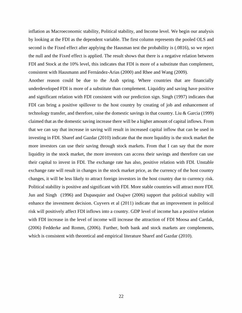
22
inflation as Macroeconomic stability, Political stability, and Income level. We begin our analysis
by looking at the FDI as the dependent variable. The first column represents the pooled OLS and
second is the Fixed effect after applying the Hausman test the probability is (.0816), so we reject
the null and the Fixed effect is applied. The result shows that there is a negative relation between
FDI and Stock at the 10% level, this indicates that FDI is more of a substitute than complement,
consistent with Hausmann and Fernandez-Arias (2000) and Rhee and Wang (2009).
Another reason could be due to the Arab spring. Where countries that are financially
underdeveloped FDI is more of a substitute than complement. Liquidity and saving have positive
and significant relation with FDI consistent with our prediction sign. Singh (1997) indicates that
FDI can bring a positive spillover to the host country by creating of job and enhancement of
technology transfer, and therefore, raise the domestic savings in that country. Liu & Garcia (1999)
claimed that as the domestic saving increase there will be a higher amount of capital inflows. From
that we can say that increase in saving will result in increased capital inflow that can be used in
investing in FDI. Sharef and Gazdar (2010) indicate that the more liquidity is the stock market the
more investors can use their saving through stock markets. From that I can say that the more
liquidity in the stock market, the more investors can access their savings and therefore can use
their capital to invest in FDI. The exchange rate has also, positive relation with FDI. Unstable
exchange rate will result in changes in the stock market price, as the currency of the host country
changes, it will be less likely to attract foreign investors in the host country due to currency risk.
Political stability is positive and significant with FDI. More stable countries will attract more FDI.
Jun and Singh (1996) and Dupasquier and Osajwe (2006) support that political stability will
enhance the investment decision. Cuyvers et al (2011) indicate that an improvement in political
risk will positively affect FDI inflows into a country. GDP level of income has a positive relation
with FDI increase in the level of income will increase the attraction of FDI Moosa and Cardak,
(2006) Fedderke and Romm, (2006). Further, both bank and stock markets are complements,
which is consistent with theoretical and empirical literature Sharef and Gazdar (2010).

23
Table 13-Poole OLS and a fixed effect for stock market development and FDI:
(Pooled
OLS) (FE)
VARIABLES FDI FDI
stock -0.413** -0.451*
(0.208) (0.218)
bank 1.218*** -0.059
(0.340) (0.552)
liquidity 0.641*** 0.526***
(0.111) (0.150)
saving 0.019*** 0.043**
(0.006) (0.016)
EX -0.147 0.920***
(0.341) (0.249)
Inflation 0.009 0.035
(0.018) (0.041)
POS -0.722*** 0.413*
(0.167) (0.207)
GDP 0.195*** 0.137**
(0.062) (0.058)
Constant 14.512*** 9.011*
(2.851) (4.842)
Observations 144 144
R-squared 0.503 0.690
Number of ids 10
country FE Yes
Year FE Yes
*** indicate significant at 1% level, ** indicate significant at 5% level, * indicate significant at 10%.
Looking at the regression from the stock perspective and applying Hausman test the result indicate
the Random effect is appropriate (.7389). The result shows that stock and FDI are negative but not
significant, Bank is positive and significant which provides long-term financing to private
corporations. Liquidity also, has a positive relation with stock market development. Further, both
bank and stock markets are complements, which is consistent with theoretical and empirical
literature Sharef and Gazdar (2010). Lastly, political risk has no significant effect on stock market
capitalization.
Checking for multicollinearity, we will apply the variance inflation factor according to Hair et al,
(2010) and Ringle et al, (2015) indicate that if VIF < 4 then it will have a low probability of

24
Multicollinearity. Based on the result from the table we can see that we will have a low probability
of multicollinearity all the variables are less than 10.
Table 14-The variance inflation factor for stock and FDI:
Variable VIF
Stock 3.36
Liquidity 3.27
POS 1.85
Inflation 1.71
Bank 1.69
Saving 1.66
GDP 1.60
EX 1.13
Mean VIF 2.03
5. Summary and Conclusion:
This paper contributes to the existing literature by providing a relation between FDI, trade, capital
formation, and economic growth in MENA countries; And whether FDI is a substitute or a
complement to the stock market capitalization? Previous research in MENA countries shows the
determinant of stock market development, however, they did not show the effect of FDI on the
stock market, and how the stock market determinant can be related to the inflow of FDI.
Therefore, in our analysis We use the panel of pooled OLS and a fixed effect for the long-
run relation. Our result indicates that FDI has a positive relation with economic growth. As the
economic growth increase, the FDI will also increase, which they support the attraction of FDI,
due to the positive spillover that will occur for the host country. However, trade has a negative
relationship with economic growth that could be due to a change in the quota of export and import
which result in negative relation. Political stability did not have any significant result with our
model, while the inflation consumer price index has a negative relation with growth which
indicates that the government needs to increase the effort to make all the essential income
adjustments for people to retain a good quality of life. The capital formation which is the
government support increase as the economic growth increase, and labor also, increase as the

25
economic growth increase. Further we add another section with education level as a proxy for
human capital our result we support what we have.
Lastly, we look at the effect of FDI on stock market development. Our results show, that
FDI and stock market development are substitutes, where countries that are riskier and financial
underdevelopment have a negative relationship between the stock market and FDI. Further,
liquidity and saving have a positive relationship with FDI. The more the stock market is liquid the
more the investors can access their savings and therefore invest in FDI. A stable nominal exchange
rate will have less currency risk and therefore attract more FDI. Lastly, GDP and political stability
have a positive relationship with FDI. An increase in the level of income will increase the attraction
of FDI, and the more the country is stable the more the inflow of FDI.

26
27
Chapter 2:
Money demand function and its Stability in MENA countries.
1.Introduction:
Recently economists present a lot of interest in studying the money demand function, and
its stability, in the long run, whether at the country level or a group of countries. Fisher (1911)
discusses the quantity theory of money that implies an increase in the money supply will increase
the price level correspondingly, the speed of money must be stable. The speed is proxied by the
linear combination of the money supply, the price level and the level of output, that establish the
stability of money demand1. That referred to the quantity theory of money which highlights the
importance of money demand stability. Since the Nobel laureate Mundell (1963) argues that the
exchange rate affects the demand for money. Economists subsequently followed this argument and
include the exchange rate in their money demand function, further, they try to explain why the
exchange rate can affect the demand for money. Arango and Hence (1981) introduce the wealth
theory they argue that depreciation of domestic currency will increase the domestic currency value.
If this increase account as an increase in wealth, the domestic resident could increase their
consumption by demanding more money. On the other hand, Bahmani and Pourheydarian (1990),
argue that depreciation in the domestic currency will result in a decrease in the domestic currency
value and therefore, depreciation in demand for money.
Following Mundell and the other pioneer worker, we aim to investigate the importance of
the Money demand function and its stability in MENA countries, and whether Import and Export
can play a role in the demand for money. MENA is referred to the Middle East and North Africa)
countries, according to James Chen (2019) MENA region account for approximately 6% of the
world population growth, 60% of the world oil reserve, and 45% of the world natural gas reserve,
therefore MENA region is the foundation of global economic stability.
In our sample, we included 15 countries (Algeria, Bahrain, Egypt, Iran, Iraq, Jordan,
Kuwait, Lebanon, Libya, Morocco, Oman, Qatar, Saudi Arabia, Tunisia, and United Arab
Emirates) We choose those countries because they share the area around the Persian Gulf. They
also, share historical, geographical and ethnical characteristics. Furthermore, there is a very limited
1The money market is at equilibrium when the money demand and money supply are at the same quantity.

28
number of empirical studies that investigate the money demand function in monitory policy in
MENA countries. Therefore, we try to fill the gap by introducing a methodology that would
address the money demand function. We use panel autoregressive distribution lag (ARDL) and we
test for cointegration, then applied the error correction model, and the pooled mean group estimator
(PMGE) by Watson (1993). Further we test the stability by applying the CUSUMSQ (CUSUM
squared). Our empirical result shows a cointegration between the variable, also, strong and stable
long-run money demand for MENA countries.
The remainder of the paper is organized as follows: Section 2 provides a literature review,
Section 3 methodology and data description, Section 4 result, Section 5 conclusion.
2.Literature review:
Many studies estimate that the demand for money is affected by the Exchange rate. Mundell (1963)
study the effectiveness of monetary policy and fiscal policy and how they are affected by the
exchange rate, and therefore, he made the argument that exchange rate has an effect on the demand
for money and he claims “ The demand for money is likely to depend upon the exchange rate in
addition to the interest rate and the level of income; this would slightly reduce the effectiveness of
a given change in the quantity of money, and slightly increase the effectiveness of the fiscal policy
on income and employment under flexible exchange rates, while, of course, it has no significance
in the case of fixed exchange rates”. Bahmani and Pourheydarian (1990), applied Mundell’s theory
by including the exchange rate in the money demand specification for Canada, Japan, and the
United States of America. They argued that when domestic currency declines or foreign currency
rises, domestic residents are expected to hold more foreign currency and less domestic currency,
this called ‘expectation effect’ can reduce the demand for money. In other words, a depreciation
in the currency may have a negative impact on the demand for money. Hassan (1992) study the
relation between credit constraint, foreign interest rate, currency depreciation, domestic income,
and inflation on the demand for money in Bangladesh. The result reveals that Bangladesh is not
the open economy, and interest rate, currency depreciation does not play a major role in the demand
for money Mcgibany and Nourzad (1995) examine the exchange rate volatility in the US money
demand for the period of 1974 to 1990. They find the exchange rate volatility has a negative effect
on the demand for money M2. Hassan, Choudhury, and Waheeduzzaman (1995) examine the
black-market exchange rate on the demand for money in Nigeria. They find that inflation, real

29
income (GDP), and opportunity cost variable the determinant of demand for money in Nigeria.
Also, a decrease in the block market will result in depreciation on the demand for money. Bahmani
and Chi Wing Ng (2002) examine the long-run demand for money in Hong Kong using an
autoregressive distributed lag (ARDL), and the CUSUM (cumulative sum) and CUSUMSQ
(CUSUM squared) they use a quarterly data for the period of 1985 to 1999. The result shows the
M2 is cointegrated with the variable and the money demand is stable. Bahmani and Rehman
(2005) examine the stability of money demand in 7 Asian countries (India, Indonesia, Malaysia,
Pakistan, the Philippines, Singapore, and Thailand). In their study, they use the CUSUM
(cumulative sum) and CUSUMSQ (CUSUM squared) tests into cointegration analysis, their
results show that real M1 or M2 monetary aggregates are cointegrated with their determinants, and
therefore the estimated parameters are unstable. Another study was done by Bahmani and Gelan
(2009) study the demand for money in 21 African countries using quarterly data from 1971 to
2004. In their study they apply the bounds testing approach to cointegration and error correction
modeling. Also, following his paper he adds the CUSUM and CUSUMQ test to the residuals of
the error correction model. The result shows that the M2 is stable in most 21 countries, which
means the demand for money is stable. Bahmani (2013) study the exchange rate volatility and how
it can affect the demand for money in 15 non-developed countries for the period of 1980 to 2009
by using annual data. In her study she used the bound testing approach, error correction model.
She finds that exchange rate volatility has a short-run effect on the demand for money M2. Long
and Bui Hien (2016) study the determinants of money demand in Vietnam between 2003 to 2014
by applying monthly data. They apply the unit root test, cointegration techniques, fully modified
ordinary least squares, the dynamic ordinary least square, and the CUSUM and CUSUMQ. The
result shows that the demand for money is stable in Vietnam. Nchor and Adamec (2016) examine
the demand for broad money and its stability in Ghana using a time series data from 1990 to 2014.
They apply the cointegration approach and the Error correction model and the CUSUM. The result
reveals that variables are cointegrated and non-stationary, and the interest rate has a short-run
effect on demand for money, while GDP has a long-run effect. Further, the demand for money was
stable in that period. Mohsen Bahmani, Haliciogl and Sahar Bahmani (2017) study the demand for
money in Turkey by assuming that exchange rate changes have an asymmetric effect on the
demand for money. They use quarterly data, and they find that the exchange rate has a short and
long-run asymmetric effect in the M1 demand for money. Bahmani and Nayeri (2017) use

30
nonlinear models and policy uncertainty in studying the demand for money in Australia. They
found that there is a significant long-run asymmetric effect on the demand for money. Bahmani,
Halicioglu and Sahar Bahmani(2017) study the demand for money in Turkish by using the
nonlinear ARDL model, and they show that exchange rate changes do have a short and long-run
asymmetric effect on the monetary aggregate M1.Aworinde and Toye (2018) examine the
asymmetric effect of the exchange rate on demand for money by using linear and nonlinear
autoregressive distribution lag (ARDL) approach using quarterly data from 1960 to 2017. The
result reveals that exchange rate changes have short and long-run asymmetric effects on demand
for money in Nigeria.
The literature has presented many studies and empirical work for the money demand, however,
there are very few studies that address the demand for money in some of MENA countries. Some
of these studies Darrat and Mutawaa (1996) study the Money demand function for the United Arab
Emirates, and they use the non-oil GDP to obtain quarterly data and estimate the error correction
model by OLS. They use the log of M1 to the log of non-oil GDP, the log of foreign interest rates,
the log of the inflation rate and nominal exchange rate plus an error correction term. The result of
the study supports the use of M1 as an intermediary target for monetary policy, also, the parameters
are stable and have their expected signs. Hassan and Aldayel (1998) study the stability of the
demand for money in 13 countries. They use two different financial system one is the Islamic
financial system while the other is a western system. They find that interest-free money is more
stable than interest-bearing money. Khatib and Towaijari (1999) use OLS to estimate Saudi
Arabia's money demand function. They regress the log of real M1 on the log of non-oil GDP,
interest rate, inflation rate, and real exchange rate from1977-1997 they use the residuals to estimate
an error correction model. They conclude that the interest rate is low and statistically non-
significant.
Harb (2004) use a panel for six Gulf Cooperation Council (GCC) to study the effect of the
exchange rate on the demand for money, from 1979 to 2000. He uses Pedroni’s cointegration test,
and group means cointegration vectors are estimated using FMOLS and Modified FMOLS. the
result shows that variables are not stationary and cointegrated. Also, he finds M1 to show better
performance than M2. Another study that had been done for the same period by Lee et al (2008)
applied the likelihood-based cointegration test in heterogeneous panels. He finds that at least two

31
cointegrated correlation in the four-dimensional vector error-correction model for the variables of
the real money balance, the real scale variable, the nominal interest rate, and the exchange rate.
Basher and Fachin (2012) examine the long-run demand for money in the GCC countries for the
period of 1980 to 2009 using panel technique. The result shows that there is stability in the money
demand for the long run. Helmi, Said, and Sbia (2015) they estimate the money demand function
for six Gulf cooperation council countries. They use quarterly data from 1980 to 2011 they apply
panel cointegration tests. They use the fully modified least square and Dynamic ordinary least
square in their analysis. They find that the variables are cointegrated and money demand is stable
in the long run.
3. Data and methodology:
Data:
We use yearly data, due to the limitation of the quarterly data. The source we obtain most of our
data is the world bank database. Following Mundell (1963) the noble prize we examine the
exchange rate to see its effect in demand for money. we add the import and export in our model to
see if it affects demand for money. Following the pioneering works of demand for money
(Bahmani and Chi Wing Ng,2002; Sahar Bahmani, 2013; Long and Bui Hien, 2016; Dennis Nchor,
and Valcav Adamec, 2016; among others)
The long-run money demand model is expressed as follows:
𝐿𝑛𝑀𝑡=𝛽0 + 𝛽1𝐿𝑛𝑌𝑡 + 𝛽2𝐿𝑛𝐸𝑥𝑡 + 𝛽3𝐿𝑛𝐼𝑀𝑃𝑡 + 𝛽4𝐿𝑛𝐼𝑋𝑃𝑡 + 𝛽5𝐼𝑡 + 𝜀𝑡 (1) Where M2 is a monetary aggregate in real term (M2); Y is the real GDP; Ex is nominal exchange
rate; IMP, and EXP are import and export; I the inflation rate. The Real GDP function as a record
of the country’s economic health and evaluate the economic development of the country and its
proxy for country income. The exchange rate account for the possibility of currency substitution,
Bahmani and Chi Wing Ng (2002) indicate that as the currency depreciates the demand for
domestic currency will decrease. For example, as the number of the MENA currency, appreciate
people are expected to hold more MENA currency, while if the MENA currency depreciate people
will hold less MENA currency, which leads to a decrease in the demand for money. The Inflation
rate measure for price changes, it used as a proxy for the opportunity cost of holding money
according to Sara Bahmani (2011) in less developed countries the interest rate is fixed by the
government, so it’s not a market-determined, therefore, using inflation will have a better result. In
an open economy, if a country imports more than it exports, there is relatively less demand for its

32
currency, so prices decline. That results in currency depreciation or lose value, as the currency
depreciates the demand for money decreases. And the opposite is true in case they export more,
the currency well appreciates and therefore demand for money will increase. M2 is a calculation
of the money supply that includes checking deposits, cash, money market securities, savings
deposits, mutual funds, and other deposits. The Ln is the natural logarithm. Appendix A has
variables explanations.
The short-run effect of demand for money is distinguished from the long-run effect. To do so, we
apply the autoregressive distribution lag (ARDL) cointegration procedure. The ARDL was
introduced by Persiaran and shin(1999) and Pesaran et al(2001) this model has couple advantages,
first, it does not need for all the variable must be Integrated of the same order it can be applied
when the variable is of order one, zero, or fractionally integrated. Lastly, the result of the ARDL
is unbiased estimates for the long run. To test for the null of no cointegration against the long-run
relationship regardless of whether the underlying variables are I (0), I (1), or fractionally
integrated. Therefore, Equation (2) specified an error correctio model representation of the ARDL
model. Following Pesaran et al (2001) bound testing approach we write (1) as (2):
𝐿𝑛𝑀𝑡= 𝛽0 + 𝑖=1𝑛1
𝛽𝑖𝐿𝑛𝑀𝑡−𝑖 + 𝑖=0𝑛2
𝑖𝐿𝑛𝑌𝑡−𝑖 + 𝑖=0𝑛3
𝑖𝐿𝑛𝐸𝑥𝑡−𝑖 + 𝑖=0
𝑛4𝑖𝐿𝑛𝐸𝑋𝑃𝑡−𝑖 +
𝑖=0𝑛5
𝑖𝐿𝑛𝐼𝑀𝑃𝑡−𝑖 + 𝑖=0𝑛5
𝑖𝐼𝑡−𝑖 +
0𝐿𝑛𝑀𝑡−1 +
1𝐿𝑛𝑌𝑡−1 +
2𝐿𝑛𝐸𝑥𝑡−1 +
3𝐿𝑛𝐸𝑋𝑃𝑡−1 +
4
𝐿𝑛𝐼𝑀𝑃𝑡−1 + 5
𝐼𝑡−1 + 𝜀𝑡 (2)
The short-run effects are then inferred by the coefficient estimates attached to all of the first-
differenced variables which are the estimates of βi, δi, i, ηi and i. The long-run effects are
inferred by the estimates of ρ1 -ρ5 that are normalized on ρ0. However, for the long-run
coefficients to be meaningful, we test for cointegration, and we must justify the joint significance
of lagged level variables as a sign of cointegration. Pesaran et al. (2001) propose using the standard
F test for the joint significance of lagged level variables. By assuming all variables to be non-
stationary, or I (1), and/or to be stationary, I (0), therefore they provide an upper bound critical
value and lower bound critical value. If the computed F-statistic falls above the upper bound
critical value, then the null of no cointegration is rejected. But if it falls below the lower bound
then the null cannot be rejected. For joint significance that establishes cointegration among the
variables, the calculated F-statistic should be greater than the upper bound critical value. From that

33
we can estimate the long-run coefficient of money demand function and the ARDL error correction
model.
Methodology:
The empirical study is divided into steps, first: after the summary statistic, and the pairwise
correlation between the variables, we apply unit root test to see if the variable contains panel unit
root to confirm the stationary of the variables. Since we have unbalanced data, we will apply the
LM-Pesaran-Shin, other tests like Levin–Lin–Chu (2002), Harris–Tzavalis (1999), Breitung (2000
and Das 2005), and Hadri Lagrange multiplier LM (2000) requires a strong balance data set.
Second, applying the panel cointegration using Pedroni (2004) to establish a cointegrating long-
term equilibrium relationship between money demand and its factors. Then I will test
multicollinearity, pooled OLS, Hausman test, fixed effect with year control. Lastly the ARDL
model with error correction and the diagnostic test, white test, LM test, RESET test, and stability
test CUSUMQ.
4.Empirical Result:
In this section we will start by providing the summary statistic and the correlation. By using the
annual data for the period between 2002 and 2016 for 15 MENA countries. We restrict our self to
annual data because of the availability of the data on an annual basis, further, we only use a 15
country because Syria and Yemen, due to the war in their country the data was not documented
after 2009 which causes missing data, therefore elimination is best.
A. The summary statistics:
We present the summary statistic for15 countries between the years of 2002 to 2016.
As we can see in the table, we have unbalanced data with a maximum of 225 observations and a
minimum of 221 observations. The GDP has the highest mean followed by inflation. Inflation has
the highest stander deviation followed by GDP; a high standard deviation of the variable may
imply that variables vary among the nations.

34
Table 15-summary statistics:
Variable Obs Mean Std. Dev Min Max
M2 221 4.673386 .3111746 2.77368 5.289307
GDP 223 25.17364 1.040356 22.9832 27.35177
NEX 224 4.656862 .1871461 3.597586 6.129116
Inflation 225 6.122725 11.12634 -26.86571 35.56745
Import
Export
225
225
3.685883
3.818836
. 396129
.4375484
2.865529
2.336548
4.545393
4.652121
B. The correlation analysis:
Table 16-Pairwise correlation:
M2 GDP NEX Inflation Export Import
M2 1.0000
GDP 0.5805*
1.0000
NEX 0.1146
0.0676
1.0000
Inflation 0.4455*
0.6941*
-0.0516 1.0000
Export
Import
0.1656*
-0.1560*
0.1499*
-0.2025*
0.1383*
0.1330*
-0.0170
-0.3086*
1.0000
0.4353* 1.0000
• The significant at 5% level
The table shows that GDP is correlated positively with M2. inflation is correlated with M2, and
GDP. Export has a positive correlation with M2, GDP, and nominal exchange rate. lastly Import
is correlated negatively with M2, GDP, Inflation, while positively with the exchange rate, and
Export. An Increase in imports will increase exporting means a more open economy.
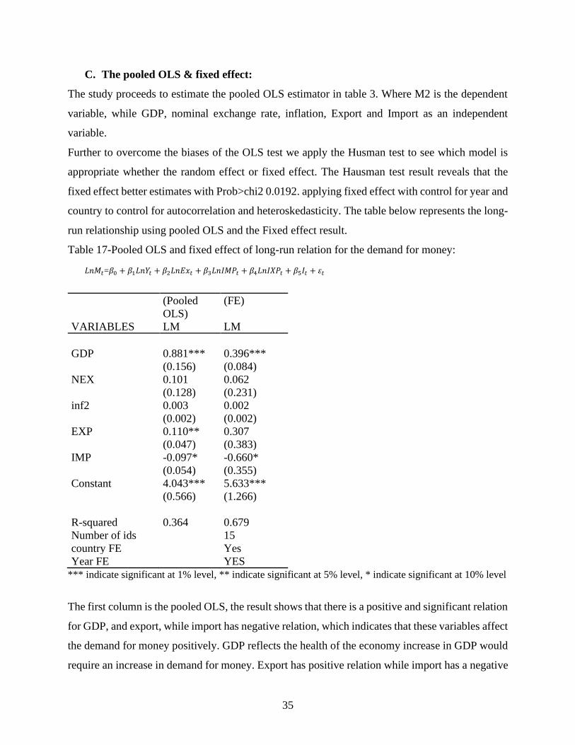
35
C. The pooled OLS & fixed effect:
The study proceeds to estimate the pooled OLS estimator in table 3. Where M2 is the dependent
variable, while GDP, nominal exchange rate, inflation, Export and Import as an independent
variable.
Further to overcome the biases of the OLS test we apply the Husman test to see which model is
appropriate whether the random effect or fixed effect. The Hausman test result reveals that the
fixed effect better estimates with Prob>chi2 0.0192. applying fixed effect with control for year and
country to control for autocorrelation and heteroskedasticity. The table below represents the long-
run relationship using pooled OLS and the Fixed effect result.
Table 17-Pooled OLS and fixed effect of long-run relation for the demand for money:
𝐿𝑛𝑀𝑡=𝛽0 + 𝛽1𝐿𝑛𝑌𝑡 + 𝛽2𝐿𝑛𝐸𝑥𝑡 + 𝛽3𝐿𝑛𝐼𝑀𝑃𝑡 + 𝛽4𝐿𝑛𝐼𝑋𝑃𝑡 + 𝛽5𝐼𝑡 + 𝜀𝑡
(Pooled
OLS) (FE)
VARIABLES LM LM
GDP 0.881*** 0.396*** (0.156) (0.084) NEX 0.101 0.062
(0.128) (0.231)
inf2 0.003 0.002 (0.002) (0.002) EXP 0.110** 0.307
(0.047) (0.383) IMP -0.097* -0.660*
(0.054) (0.355) Constant 4.043*** 5.633*** (0.566) (1.266)
R-squared 0.364 0.679 Number of ids 15
country FE Yes Year FE YES
*** indicate significant at 1% level, ** indicate significant at 5% level, * indicate significant at 10% level
The first column is the pooled OLS, the result shows that there is a positive and significant relation
for GDP, and export, while import has negative relation, which indicates that these variables affect
the demand for money positively. GDP reflects the health of the economy increase in GDP would
require an increase in demand for money. Export has positive relation while import has a negative

36
relation, indicating that as the economy opens its doors for trade exporting good will increase the
demand for money, how? By exporting goods, the value of the currency will increase, therefore
appreciate the demand for money. On the other hand, importing will reduce the values of the
currency, and therefore depreciated the demand for money. The exchange rate has positive but not
significant as the exchange rate appreciates people will hold more of the currency and the demand
for more money. The second column show, the result of the fixed effect where GDP is positive
and significant the nominal exchange rate is positive but not significant. Import has a negative
relation the more they import the value of the currency would depreciate and therefore decrease
the demand for money.
Checking for multicollinearity, we will apply the variance inflation factor according to Hair et al,
(2010) and Ringle et al, (2015) indicate that if VIF < 10 then we will have a low probability of
Multicollinearity. Based on the result from the table we can see that we will have a low probability
of multicollinearity.
Table 18-Variance inflation factor:
Variable VIF
Export 1.35
Import 1.41
GDP 2.13
NEX 1.20
inflation 2.16
Mean VIF 1.65
In the following section we will do the ARDL model and its specification, first we will start with
the unit root test followed by the cointegration test. We apply the cointegration test to see if the
variables are cointegrated or not, if the variables are cointegrated then we apply the error correction
model.
D. The unit root test and panel cointegration test:
We apply the LM Psarian shin for our unbalanced data. The hypothesis assumes that all panels
contain a unit root, while the alternative hypothesis is some cross-sections do not contain a unit

37
root (stationary). The result indicates that the series are more likely to have a panel unit root in
their levels means nonstationary panel.
Perform the LM person unit root test with (1) lag, and first different:
Table 19-Unit root test stationary:
LM Persian unit root test Level First different
M2 Not stationary Stationary
Export Not stationary stationary
NEX Not stationary Stationary
INFLATION Stationary
GDP Stationary
Import Stationary
The result shows that M2 and nominal exchange rates are stationary after taking the first difference
and 1 lag, while the Tarde, GDP, and inflation are stationary at the one lag level. Appendix (B)
E. The cointegration test:
After checking the integration of our variable at order one, we follow by applying the cointegration
test. Pedroni (2004) and Kao (1999) tests are performed to verify the presence of the long-run
relationship between the variable the test results are displayed in table 17. Pedroni and Kao
cointegration test revealed that all the variable rejects the null hypothesis of no cointegration at the
1% level and 10% level. We can conclude that long-run money demand exists for the panel where
all the variables are cointegrated. Appendix c.
Table 20-Pedroni and Kao cointegration test:
Pedroni cointegration test: Statistic
Modified Phillips-Perron t 3.2039***
Phillips-Perron t -10.0272 ***
Augmented Dickey-Fuller t -7.9572 ***
Kao cointegration test:
ADF 1.5090*
*** * indicate significant at 1%, 10% level.

38
F. The ARDL model:
Following the literature works of demand for money (Bahmani-Oskooee and Chi Wing Ng,2002;
Sahar Bahmani, 2013; Long and Bui Hien, 2016; Dennis Nchor, and Valcav adamec, 2016; among
others) we apply the Autoregressive distribution lag (ARDL) cointegration procedure by Persons
(2001). The cointegration result of Padroni shows that the variables are cointegrated, and the
relation of the long run exist, so we have to add an error correction term in the model.
Table 21-ARDL model short-run vs long-run relationship:
VARIABLES Bahrain KSA Kuwait Qatar UAE Oman Jordan
ECT -1.383*** -0.721*** -1.229*** -0.568*** -0.307 -1.579*** -0.927***
(0.177) (0.206) (0.183) (0.167) (0.387) (0.170) (0.211)
D.LGDP 0.469 0.074 0.092 0.073 0.086 -0.396 -2.346***
(0.330) (0.489) (0.218) (0.239) (0.467) (0.344) (0.649)
D.LNEX 2.377*** 0.685 1.387** 1.131 -0.383 1.412*** 1.454***
(0.511) (0.783) (0.673) (0.697) (1.181) (0.326) (0.557)
D.inf2 0.005** 0.007** 0.000 0.001 0.005 -0.002 0.009*
(0.002) (0.003) (0.002) (0.002) (0.006) (0.002) (0.005)
D.LEXP 1.106** -0.467 0.223 0.122 -0.236 0.499*** 1.196
(0.528) (0.591) (0.467) (0.351) (0.769) (0.185) (0.738)
D.LIMP -0.978** 0.055 0.682*** -0.651*** -0.527 0.363*** -0.646
(0.426) (0.225) (0.208) (0.213) (0.415) (0.095) (0.440)
16.492*** 8.798*** 14.691*** 6.741*** 3.790 18.807*** 11.545***
Constant (2.247) (2.524) (2.537) (2.062) (4.826) (2.078) (2.624)
Panel B: long run for each country and diagnostic:
GDP 0.455 0.400 -0.302 1.276** 0.572 -0.018 -3.310**
(1.089) (0.868) (0.510) (0.432) (0.629) (1.528) (1.321)
LNEX 1.000 -0.141 -0.424 -0.444 -1.221*** -0.507 0.055
(0.592) (0.779) (1.165) (0.656) (0.301) (0.961) (0.409)
inf2 0.004 0.001 0.009 -0.007 -0.005 0.005 0.030**
(0.013) (0.011) (0.010) (0.005) (0.008) (0.014) (0.012)
LEXP 1.695 0.425 0.116 -0.198 -0.464** 0.468 0.531
(0.904) (0.247) (0.361) (0.238) (0.135) (0.412) (0.312)
LIMP -1.461* -0.051 -0.517 -0.729** -0.725** -0.729* -0.141
(0.670) (0.219) (0.363) (0.216) (0.222) (0.341) (0.251)
R-squared 0.889 0.859 0.857 0.924 0.933 0.726 0.904

39
Continue Table 22-ARDL model short-run vs long-run relationship:
Panel C:
Diagnostic:
White test
LM
RESET
CUSUMQ
0.369
0.4549
0.9912
stable
0.3738
0.9534
0.3828
stable
0.3738
0.0520
0.3302
stable
0.3738
0.016
0.0357
stable
0.3738
0.0653
0.2475
stable
0.3738
0.0831
0.5526
stable
0.3738
0.0482
.1282
Not
stable
VARIABLES Algeria Egypt Iran Iraq Lebanon Libya Tunisia Morocco
ECT -0.849*** -0.432** -0.028 -1.777*** -0.606*** -0.211*** -0.779*** -1.456***
(0.254) (0.200) (0.133) (0.215) (0.114) (0.074) (0.266) (0.270)
D.LGDP -0.925** 0.091 0.086 -1.017*** 0.734** 0.714*** 0.685 1.040***
(0.414) (0.590) (0.409) (0.321) (0.292) (0.123) (0.720) (0.400)
D.LNEX 1.908*** 0.576 -0.131 0.081 1.072*** 0.066 1.492 -10.075***
(0.585) (0.404) (0.165) (0.598) (0.371) (0.630) (1.588) (2.943)
D.inf2 0.007*** 0.006 0.007 0.003* -0.033*** -0.001 -0.027 -0.040*
(0.002) (0.008) (0.006) (0.002) (0.004) (0.002) (0.024) (0.023)
D.LEXP -0.057 0.328 0.113 -1.007*** -0.366* 0.689*** 1.695 0.328
(0.795) (0.428) (0.545) (0.386) (0.195) (0.228) (1.452) (0.617)
D.LIMP -0.211 -1.194* -0.132 -0.049 0.617 -0.058 -0.866 -0.215
(0.365) (0.644) (0.430) (0.115) (0.386) (0.201) (1.429) (0.536)
10.361*** 5.281** 0.261 22.109*** 7.347*** 2.315*** 9.395*** 17.867***
Constant (3.069) (2.467) (1.591) (3.256) (1.415) (0.892) (3.238) (3.888)
Panel B: long run relation:
GDP -0.527 1.227 0.099 2.352 3.582 3.411 -0.030 0.137
(0.380) (1.396) (0.497) (1.818) (3.486) (2.782) (0.604) (0.591) LNEX 0.277 1.355 0.490** -0.820 0.512 18.415 0.506 -5.187*
(0.604) (2.007) (0.175) (1.221) (2.219) (13.744) (0.660) (2.639) inf2 0.014* 0.009 0.004 -0.016 -0.057 -0.007 -0.006 0.000
(0.006) (0.023) (0.007) (0.013) (0.047) (0.018) (0.029) (0.034) LEXP 0.230 -0.280 0.017 -0.546 -0.331 3.181* 0.498 -0.382
(0.198) (1.517) (0.630) (0.860) (0.802) (1.470) (0.774) (0.799) LIMP -0.006 -0.501 0.064 0.620 0.651 -1.624 -0.462 -0.426
(0.206) (2.305) (0.458) (0.550) (1.677) (0.907) (1.002) (0.421) R-
squared 0.858 0.541 0.565 0.899 0.653 0.943 0.678 0.694

40
Continue- Table 23-ARDL model short-run vs long-run relationship:
Panel C:
Diagnostic:
White test
LM
RESET
CUSUMQ
0.3738
0.6085
0.8492
stable
0.3738
0.2953
0.5935
stable
0.3738
0.0895
0.1321
stable
0.3575
0.3672
0.2751
Stable
0.3738
0.4071
0.0068
stable
0.3738
0.3976
0.9969
Stable
0.3738
0.0309
0.8688
Stable
0.3738
0.0029
0.9113
Not stable
*** indicate significant at 1% level, ** indicate significant at 5% level, * indicate significant at 10%
Table 18 presents the short-run coefficient estimate, in most cases for each first different variable
there is at least one significant coefficient estimate, implying that GDP, inflation, exchange rate,
Export, and import do have short-run effects on the demand for money in most 15 MENA
countries. Further, the error correction term (ECT) it is important to have a negative coefficient
obtain for ECT which support the cointegration and reflect the adjustment toward the long-run
equilibrium, further the ECT in the short run table denote that there is a long-run cointegration at
1% level, so any divination from the long run is corrected .868 for Bahrain and at .405 for Kuwait
and the same for the rest of the countries. It is interesting to say that for Lebanon, Algeria, Bahrain,
Kuwait, Oman, and Jorden the exchange rate is positive and significant in the short run. While its
negative for Morocco that means in the short-run appreciation in the exchange rate will increase
the demand for money, on the other hand depreciation will result in decreased demand for money.
For GDP it’s positive and significant for Libya, Morocco, and Lebanon; however, it is positive but
not significant for the rest of the countries except, Jordan, Algeria, and Iraq is negative significant
in the short-run, increase in GDP will increase the demand for money, so people can be able to
meet the requirement of a good life. Inflation has a positive and significant results for Bahrain,
KSA, Jordan, Algeria, and Iraq, while its negative for Lebanon and Morocco in the short-run
increase in inflation will increase the demand for money. Export has a positive and significant
relation with Bahrain, Libya and Oman, increase exporting the goods will support the value of the
currency and result in an appreciation of the currency and increase the demand for it, its negative
for Iraq and Lebanon. Import has a positive and significant relation with Bahrain, Qatar, and Egypt,
while it’s positive for Oman and Kuwait. An increase in the import of goods will weaken the value
of the currency and therefore reduce the demand for money.

41
We can say that for the long run a percentage change in the exchange rate is associated with an
increase in the demand for money in Iran, most of the other countries we can see a positive relation
which indicates an increase in the exchange rate will increase the demand for money. While UAE
and Morocco have negative and significant relation, have negative relation indicate that a
percentage change in the exchange rate is associated with a decrease in the demand for money.
The percentage change in inflation is associated with an increase in the demand for money Jorden
and Algeria. Further Qatar has positive and significant results while other countries are positive
only, an increase in GDP will increase the demand for money, except for Jorden has negative and
significant Oman, Kuwait. Algeria, Tunis has a negative result with GDP. For exporting its
positive and significant for Libya, while negative for UAE. Importing has a negative and
significant relation with Bahrain, Qatar, UAE, Oman, and most of the countries has negative
relation, which indicates the more they import goods from other countries the more they will
weaken their currency value and therefore decrease the demand for money.
To answer the question of whether the short-run effect is permanent or transitory? we compare
both panels. For GDP I can say the negative sign followed for Jorden, Oman, and Algeria. The
inflation we can say that it was positive in the short run for Jordan, and Algeria. For import it cries
for Bahrain, Qatar, and Oman. It is clear the short-run effect does not carry to the long-run effect
especially the exchange rate and exporting goods and services.
For the diagnostic test, it is necessary to test for cointegration to make sure that the variables are
cointegrated, and the result shows that the variables are significantly cointegrated at the 1% level.
Also, apply the ECT error correction term is important to have a negative and significant
coefficient obtain for ECT which supports the cointegration and reflects the adjustment toward the
long-run equilibrium.
Furthermore, we apply three other diagnostic statistics, the Lagrange multiplier LM test to test for
the correlation (relation between the error correction and its values) the presences of
autocorrelation, the Ramsey RESET suggest that the model is well specified, and white test for
heteroscedasticity. Both of the first tests are distributed as one degree of freedom. The result in
most cases they fail to reject the null hypothesis and the as can be seen in the diagnostic section in
the table, implying free no heteroscedasticity, and a correctly specified model. For autocorrelation
we can see there is an autocorrelation problem in most cases. Furthermore, following Bahmani’s

42
papers, we apply the CUSUMSQ test to assess the parameter stability, the result reveals that most
the country indicates the absence of any instability of the coefficient because the plot of
CUSUMSQ statistic falls inside the critical band of the 5% confidential interval of parameter
stability except for, Jorden and Morocco.
Figure 3- Represent the stability of the Money demand graph: (Bahrain, KSA, Kuwait, Qatar,
UAE, Oman, Jourdan, Algeria, Egypt, Iran, Iraq, Lebanon, Libya, Tunisia, Morocco) respectively:

43
The graphs show the stability of the money demand in MENA countries as follows (Bahrain, KSA, Kuwait,
Qatar, UAE, Oman, Jourdan, Algeria, Egypt, Iran, Iraq, Lebanon, Libya, Tunisia, Morocco) respectively.
For Jorden we can see that it was above the 5% boundary Before 2010 tell 2012, then it returns to be stable.
Morocco is, above the 5% boundary before 2010 up until 2012 then it returns to be stable.
The other countries like (Bahrain, Egypt, Iran, Jourdan, KSA Kuwait, Lebanon, Libya, Oman, Qatar, UAE)
We can see that it is stable for the period.
5. Summary and conclusion:
It is well known by Mundell and others, that there is three important determinant for the demand
for money, they are income (GDP), Interest rate, in our paper we replace it with inflation due to
limitation of the interest rate were its fixed by the government and will not give an accurate result,
and lastly exchange rate. We add to the literature by examining 15 MENA countries, from 2002
to 2016 using annual data. Further, in our paper we add Exporting and Importing goods. We were,
interested to see if it affects in the long run, the result indicates that in the long run import has a
negative and significant effect at 10% level for the Fixed effect, and pooled OLS. Which indicates
in an open economy where the percentage of Import increase may result in a decrease in money
demand, how? By favoring the product of the other country, which weakens the currency of the
same country and therefore depreciation in the demand for money. In other words, if a country
imports more than it exports, there is reasonably less demand for its currency, so prices should
decrease. The case of currency depreciates or loses its value, the currency depreciates the demand

44
for money decline. GDP in Pooled OLS and Fixed effect models have a positive and significant
result in the long run. GDP account for economic health increase in GDP (income)will result in an
increased demand for money. Same for inflation, where it has positive relation only an increase in
the price level will increase demand for money were citizens will require to increase their income
to meet the changes in the price, and the opposite is right. For the exchange rate it is interesting to
say that it is not significant in the Pooled OLS, or fixed effect but its positive an appreciation in
the exchange rate will result in appreciation for the domestic currency. However, the result will
vary from one country to another.

45
References:
Chapter 1:
Acquah-Sam, E. (2016). Determinants of capital market development in Ghana. European
Scientific Journal, 12(1), 251-270.
Ayunku, P.E. & Etale, L.M. (2015). Determinants of stock market development in Nigeria: A co-
integration approach. Advances in Research, 3(4), 366-373.
Amelia Budiharto, Suyanto, Aluisius Hery Pratono ( 2017), The Relationship between Economic
Growth, FDI, Trade, Labor, Capital Formation in Indonesia, Advances in Economics, Business
and Management Research (AEBMR), volume 35.
Adhikary. (2011). FDI, trade openness, capital formation, and economic growth in Bangladesh: A
linkage analysis. International Journal of Business and Management, 6 (1), 1-21.
Asaolu, T.O. & Ogunmuyiwa, M.S. (2011). An econometric analysis of the impact of
macroeconomic variables on stock market movement in Nigeria. Journal of Business Management,
3(1), 72-78.
Beghin. D, Roland-Holst. D, Van der Mensbrugghe. (2006). Trade and the Environment in General
Equilibrium: Evidence from Developing Economies. Berlin: Springer Science & Business Media.
Belloumi. (2014). The relationship between trade, FDI and economic growth in Tunisia: An
application of the ARDL model. Economic System, 38 (1), 269-287.
Ben Naceur, S., Ghazouani, S., and Omrani, M. (2007). The determinants of stock market
development in the MENA region. Managerial Finance, 33 (7), 477-489.
Boyd, J.H., Levine, R., and Smith, B.D. (2001). The impact of inflation on financial sector
performance. Journal of Monetary Economics, 47 (2), 221-248.
Blomstrom, M., Lipsey R. and Zejan M. 1992. “What explains Developing Country Growth?”,
NBER Working Paper Series, No. 4132.
Breitung, J. (2000), The local power of some unit root tests for panel data. In: Baltagi, B., editor.
Nonstationary Panels, Panel Cointegration, and Dynamic Panels, Advances in Econometrics. Vol.
15. Amsterdam: JAI. p161-178.
Carkovic, M. and Levine, R., 2002. “Does Foreign Direct Investment Accelerate Economic
Growth?”. University of Minnesota. Working Paper.
Cuyvers, L., Soeng, R., Plasmans, J. and Bulcke, D. V. D. (2011). Determinants of foreign direct
investment in Cambodia. Journal of Asian Economics , 22, 222-234

46
Cohen. and Levinthal. (2012). Innovation and Learning: The Two Faces of R&D. Economic
Journal, 99 (2), 569-596.
Dupasquier, C. and Osajwe, P. N,. (2006). Foreign direct investment in Africa: Performance,
challenges, and responsibilities. Journal of Asian Economics, 17 (2), 241-260.
De Mello Jr. and Luiz, R. (1999). Foreign direct investment-led growth evidence from time series
and panel data. Oxford Economics Papers, 51 (2), 133–151.
Dev, K. & Shakeel, S.F. (2013). Determinants for the growth of stock market. The International
JISR-MSSE, 11(2), 71-82.
Edwards, S. (1992). Trade orientation, distortions and growth in developing countries. Journal of
Development Economies, 39, 31-57.
Fisher, I. (1911) The purchasing power of money: Its determination and relation to credit, interest,
and crises. New York: Macmillan, reprinted, New York, Augustus M. Kelley, 1963.
Fedderke, J. W. and Romm, A. T. (2006). Growth impact and determinants of foreign direct
investment into South Africa, 1956-2003. Economic Modelling , 23, 738-760.
Islam, F.T., Mostofa, M.S. & Tithi, A.A. (2017). Macroeconomic and institutional determinants
of capital market performance in Bangladesh: A case of Dhaka stock exchange. International
Journal of Academic Research in Accounting, Finance and Management Sciences, 7(1), 306-311.
Harris, R. and Sollis, R. 2003. “Applied Time Series Modelling and Forecasting”. Wiley, West
Sussex.
Hair (2010), J. F. Jr., Anderson, R. E., Tatham, R. L. & Black, W. C. (1995). Multivariate
Data Analysis (3rd ed). New York: Macmillan.
Ho and Ike (2017). Determinants of stock market development: a review of the literature. Studies
in Economics and Finance, 34(1): 143-164.
Hausmann, R. and Fernandez-Arias, E. (2000). Foreign direct investment: good cholesterol? Inter-
American Development Bank Working Paper 417, New Orleans, April.
Jun, K. W. and Singh, H. (1996). The determinants of foreign direct investment in developing
countries. Transnational Corporations , 5, 64-104.
Jeffus et al (2005), FDI and stock market development in selected Latin American countries. Latin
American Financial Markets: Developments in Financial Innovations (International Finance
Review). 5: 35-44.
Kaehler, J., Weber, C.S. & Aref, H.S. (2014). The Iraq stock market: Development and
determinants. Review of Middle East Economics and Finance, 10(2), 151-175.
47
Kao, C. (1999), Spurious regression and residual-based tests for cointegration in panel data.
Journal of Econometrics, 90(1), 1-44.
Kao, C., Chiang, M.H. (2000), On the estimation and inference of a cointegrated regression in
panel data. In: Baltagi, B., editor. Nonstationary Panels, Panel Cointegration, and Dynamic
Panels, Advances in Econometrics, 15, 161-178.
Kalim, R. & Shahbaz, M. (2009). Impact of Foreign Direct Investment on Stock Market
Development: The Case of Pakistan. Global Conference on Business and Economics, 978-0-
9742114-2-7
Lee, C.C., Chang, CP., Chen, PF. (2008), Money demand function versus monetary integration:
revisiting panel cointegration among GCC countries. Mathematics and Computers in
Simulation, 79, 85-93.
Levin, A., Lin, C., Chu, C.J. (2002), Unit root tests in panel data: asymptotic and finite-sample
properties. Journal of Econometrics, 108(1), 1-24.
Liew, V, K-S., (2004). "What lag selection criteria should we employ?", Economics Bulletin,
33(3), pp. 1-9.
Moosa, I. A. and Cardak, B. A. (2006). The determinants of foreign direct investment: an
extreme bounds analysis. Journal of Multinational Financial Management, 16, 199-211.
Mondher Cherif and Kaouthar Gazdar (2010). Institutional and Macroeconomic determinant of
stock market development in MENA region: New Results from a panel Data analysis, The
International Journal of Banking and Finance, Vol. 7. Number 1: 2010: 139-159
Pedroni, P. (2004), Panel cointegration, asymptotic and finite sample properties of pooled time
series tests with an application to the PPP hypothesis. Economy Theory, 20, 597-625.
Paugel, A. T. (2007). International Economics. McGraw-Hill Irwin: New York, USA.
Romer. (1986). Increasing returns and long-run growth. Journal of Political Economy, 94 (5),
1002-1037.
Romer (1990). Endogenous technological change. Journal of Political Economy, 98 (1), 71–102.
Rhee, G.S. and Wang, J. (2009). Foreign institutional ownership and stock market liquidity:
evidence from Indonesia, Journal of Banking and Finance, 33: 1312-1324.
Lucas. (1988). On the mechanics of economic development. Journal of Monetary Economics, vol.
22, no. (1), 3-42.
Yucel, F., 2009. Causal Relationships Between Financial Development, Trade Openness and
Economic Growth: The Case of Turkey. Journal of Social Sciences 5, 33-42.

48
Nurkse. (1953). Problems of Capital Formation in Underdeveloped Countries. Basil Blackwell
Publisher: Oxford.
Nguyen, P.D. & Hanh, V.T.H. (2012). Determinants of stock market development in Southeast
Asian countries. Journal of Economics and Development, 44(1), 101-112.
Naser I Abumustafa (2016) Investigating the Arab stock markets during Arab spring, Journal of
Asset Management, September 2016, Volume 17, Issue 5, pp 313–318.
Safitri. (2014). International trade and foreign direct investment in Indonesia. Buletin Ilmiah
Litbang Perdagangan, 8 (1), 93-116.
Shahbaz, M. & Rahman, M.M. (2010). Foreign capital inflows-growth nexus and the role of
domestic financial sector: An ARDL co-integration approach for Pakistan. Journal of Economic
Research, 15(3), 207-231.
Stijn Claessens, Daniela Klingebiel, and Sergio L. Schmukler (2001). FDI and Stock Market
Development: Complements or Substitutes? Journal of Economics and Development.
Sekhri, V., & Hague, M. (2015). Impact of Foreign Investments on Indian Stock Market: An
Empirical Stud. Asian Journal of Research in Banking and Finance, 5(6): 168-185.
Simeon Nanovsky (2015) The Impact of Oil Prices on Trade with an Application to the Euro’s
Trade Effect,
Yusof, W.F.W. & Guima, I.J. (2015). Stock market development of Middle East and North Africa
(MENA) region. International Journal of Business and Economics Research, 4(3), 163-171.
World Bank. (2012). World Development Indicators: CD-ROM 2004. Washington, D.C.: The
World Bank.

49
Chapter 2:
Bahmani-Oskooee M, Pourheydarian M (1990) Exchange rate sensitivity of the demand for
money and effectiveness of the fiscal and monetary policies. Appl Econ 22:917–925
Bahmani-Oskooee, M., Rehman, H. (2005), Stability of the money demand function in Asian
developing countries. Applied Economics, 37, 773-792.
Bahmani-Oskooee and Raymond Chi Wing Ng (2002), long run demand for money in Hong
Kong: An Application of the ARDL model, Journal of economic and finanace. Volume 1.
#2,2247-255.
Bahmani-Oskooee and Maharouf Oyolola (2007), Export Growth and output growth: an
application of bounds testing approach, Journal of economic and finance. Volume 31. #1
Bahmani-Oskooee, M., Gelan, A. (2009), How stable is the demand for money in African
countries. Journal of Economic Studies, 36(3), 216-235.
Bahmani-Oskooee, M., Rehman, H. (2005), Stability of the money demand function in Asian
developing countries. Applied Economics, 37, 773-792.
Bahmani-Oskooee and Majid Maki Nayeri (2017) policy uncertainty and the demand for money
in Australia: an asymmetry Analysis, Journal of economic and finance. Volume 3. #1
Bahmani- Oskooe and Ferda Halicioglu and sahar Bahmani (2017) Do exchange rate changes
have symmetric or asymmetric effect on the demand for money in Turkey? Applied Economics
49:42,4261-4270.
Bahmani Sahra (2013) Exchange rate volatility and demand for money in less developed
countries. J Econ Finance (2013) 37:442–452
Basher, S., Fachin, S. (2012), Investigating long-run demand for broad money in the Gulf Arab
Countries, DSS Empirical Economics and Econometrics, Working Papers Series, DSS-E3 WP
2012/6, La Spienza University.
Breitung, J. (2000), The local power of some unit root tests for panel data. In: Baltagi, B.,
editor. Nonstationary Panels, Panel Cointegration, and Dynamic Panels, Advances in
Econometrics. Vol. 15. Amsterdam: JAI. p161-178.
Darrat, A., Mutawa, A. (1996), Modeling money demand in the United Arab Emirates. The
Quarterly Review of Economics and Finance, 36(1), 65-87.
Dennis Nchor, and Valcav adamec (2016) investigate the stability of money demand in Ghana,
Social and Behavioral Sciences 220 (2016) 288 – 293.

50
Fisher, I. (1911) The purchasing power of money: Its determination and relation to credit,
interest, and crises. New York: Macmillan, reprinted, New York, Augustus M. Kelley, 1963
Hair (2010), J. F. Jr., Anderson, R. E., Tatham, R. L. & Black, W. C. (1995). Multivariate
Data Analysis (3rd ed). New York: Macmillan.
Hassan, M. Kabir, Benito Sanchez and Jung-Suk Yu, (2011) “Financial Development and
Economic Growth in the Organization of Islamic Conference Countries,” Journal of King Abdul
Aziz University-Journal of Islamic Economics, Volume 24, No. 1, pp: 145-172, [SCOPUS].
Hassan, M. Kabir and Adnan Q. Al-Dayel, (1998/1999)"Stability of Money Demand Under
Interest-Free Versus Interest-Based Banking System," Humanomics, Vol. 15, No.4, and Volume
15, No. 1, 167-186, [ABDC,SCOPUS]
Hassan, M. Kabir, M. M. Islam and A. Najibullah (1995), "The Role of Black-Market Exchange-
Rate Expectations in the Demand for Money in SAARC Countries: An Empirical Investigation",
as chapter nine in International Finance in the New World Order, edited by Peter H. Gray and
Sandra Richard, Pergamon Press 1995: 119-130.
Hassan, M. Kabir, K. Choudhury and M. Waheeduzzaman, "On Black Market Exchange Rate
and Demand for Money in Developing Countries: The Case of Nigeria," Atlantic Economic
Journal, Vol. 23, No.1, March 1995., [ABDC, ABS, SCOPUS]
Hassan, M. Kabir, M. Mahmud Khan and M. Badrul Haque, (1993) "Financial Development and
Income Velocity of Money in Bangladesh," The Bangladesh Development Studies, Vol.21, No.1,
15-27. [ABDC, SCOPUS]
Hassan, M. Kabir, "An Econometric Analysis of Credit Constraint, Foreign Interest Rates and
Currency Depreciation in the Demand for Money in Bangladesh," Bangladesh Development
Studies, Vol.20, No.4, December 1992: 25-45. [ABDC, SCOPUS]
Lee, C.C., Chang, CP., Chen, PF. (2008), Money demand function versus monetary integration:
revisiting panel cointegration among GCC countries. Mathematics and Computers in Simulation,
79, 85-93.
Levin, A., Lin, C., Chu, C.J. (2002), Unit root tests in panel data: asymptotic and finite-sample
properties. Journal of Econometrics, 108(1), 1-24.
Harb, N. (2004), Money demand function: a heterogenous panel application. Applied
Economics Letters, 11, 551-555.
Kao, C. (1999), Spurious regression and residual-based tests for cointegration in panel data.
Journal of Econometrics, 90(1), 1-44.
Kao, C., Chiang, M.H. (2000), On the estimation and inference of a cointegrated regression in
panel data. In: Baltagi, B., editor. Nonstationary Panels, Panel Cointegration, and Dynamic
Panels, Advances in Econometrics, 15, 161-178.
51
Khatib-Kswani, M., Towaijari, H.A. (1999), Cointegration error correction and the demand for
money in Saudi Arabia. Economia- Internazionale, 52(3), 299-308.
Mundell AR (1963) Capital mobility and stabilization policy under fixed and flexible exchange
rates. Can J Econ Polit Sci 29(4):475–85.
Mcgibany JM, Nourzad F (1995) Exchange rate volatility and the demand for money in the U.
S. Int Rev Econ Finance 4:411–425.
Mohsen Bahmani-Oskooee, Ferda Halicioglu & Sahar Bahmani (2017) Do exchange rate
changes have symmetric or asymmetric effects on the demand for money in Turkey? Applied
Economics.
Olakelan Bashir Aworinde and Ishola Rufus Akintoye (2018) DO exchange rate changes have
symmetric or asymmetric effect on money demand in Nigeria?
Pham Long and Bui Hien (2016) Determinants and stability of demand for money in Vietnam.
Pedroni, P. (2004), Panel cointegration, asymptotic and finite sample properties of pooled time
series tests with an application to the PPP hypothesis. Economic Theory, 20, 597-625.
Ringle, Christian M., Wende, Sven, & Becker, Jan-Michael. (2015). SmartPLS 3. Bönningstedt:
SmartPLS. Retrieved from smarpls.com
Steven M. Suranovic (1996) International finance theory and policy, Book
World Bank. (2012). World Development Indicators: CD-ROM 2004. Washington, D.C.: The
World Bank.
Zirek, Duygu, Fusun Celebi and M. Kabir Hassan (2016), “The Islamic Banking and Economic
Growth Nexus: A Panel VAR Analysis for Organization Islamic Cooperation (OIC) Countries,”
Journal of Economic Cooperation and Development, Volume 37, No 1, April 2016 [SCOPUS]

52
Appendix:
chapter 1:
a) Variable explanation and sources:
Variable Definition Proxy Resource
FDI Foreign direct investment refers to direct investment equity flows
in the reporting economy. Data are in current U.S. dollars.
FDI net
investment
World bank
Trad Openness Trade is the sum of exports and imports of goods and services
measured as a share of gross domestic product.
Trade World bank
Capital formation Gross fixed capital formation (formerly gross domestic fixed
investment) includes land improvements (fences, ditches, drains,
and so on); plant, machinery, and equipment purchases; and the
construction of roads, railways, and the like, including schools,
offices, hospitals, private residential dwellings, and commercial
and industrial buildings. Data are in current U.S. dollars.
.
Government
support
World bank
Labor force Labor force comprises people ages 15 and older who supply labor
for the production of goods and services during a specified period.
Labor /GDP. To get the labor growth
Labor growth World bank
GDP per capita GDP per capita is gross domestic product divided by midyear
population. Data are in current U.S. dollars.
Economic
growth
World bank
Inflation Inflation as measured by the consumer price index reflects the
annual percentage change in the cost to the average consumer of
acquiring a basket of goods and services that may be fixed or
changed at specified intervals, such as yearly.
Macroeconomic
stability
World bank

53
Political Stability
and Absence of
Violence/Terrorism
captures perceptions of the likelihood that the government will be
destabilized or overthrown by unconstitutional or violent means,
including politically motivated violence and terrorism.
Country
stability
World bank
Liquidity Stock market liquidity, how investors can access their saving. Stock market
traded value (% of
GDP)
World bank
Savings Gross domestic savings are calculated as GDP less final consumption expenditure (total consumption).
Gross domestic
savings (% of
GDP)
World bank
Stock
Stock market development, value of listed shares as % GDP.
Stock market
capitalisation
(% of GDP)
World bank
Bank Banking sector development, refers to financial resources provided
to the private sector by other depository corporations, such as
through loans, purchases of nonequity securities, and trade credits
and other accounts receivable
Domestic credit
to private sector
by banks (% of
GDP)
World bank
GDP Gross domestic product, market size and level of income Level of
income
World bank
Nominal exchange
rate
Local currency against the United States Dollar (US $)
EX World bank
B:
Stock market development as dependent variable:
(Pooled
OLS) (RE)
VARIABLES Stock stock
Bank 0.805*** 0.717***
(0.127) (0.179)
Liquidity 0.455*** 0.477***
(0.032) (0.096)

54
saving 0.009*** 0.008
(0.002) (0.007)
EX -0.184 -0.041
(0.138) (0.145)
Inflation -0.023*** -0.020
(0.007) (0.014)
POS -0.177** -0.150
(0.071) (0.195)
LGDP -0.114*** -0.128***
(0.024) (0.033)
FDI -0.069** -0.106
(0.035) (0.065)
Constant 5.268*** 5.742***
(1.184) (1.533)
Observations 144 144
R-squared 0.711
Number of id 10
Chapter 2:
a) Variable explanation and sources: Variables Definition proxy Source
M2 a monetary aggregate in
real term.
Proxy for the
money demand
World Bank
national accounts
data, and OECD
National Accounts
data files.
Export . World Bank
national accounts
data, and OECD
National Accounts
data files.
+
GDP It’s functions as a
comprehensive scorecard
of the country’s economic
health and evaluate the
economic development of the country.
Proxy for country
income.
World Bank
national accounts
data, and OECD
National Accounts
data files.
+

55
NEX the number of units of the
domestic currency that
can purchase a unit of a
given foreign currency
Proxy for
currency
substitution
World Bank
national accounts
data, and OECD
National Accounts
data files.
+
Inflation Inflation as measured by
the annual growth rate of
the GDP implicit deflator
shows the rate of price
level change in the
economy as a whole.
Proxy for
opportunity cost
of holding money
World Bank
national accounts
data, and OECD
National Accounts
data files.
+
B) Explanation of variables on demand for money.
• Explanation for inflation: by Steven Suranovic (1996).
“Suppose the money market is originally in equilibrium at point A in the adjoining diagram with
real money supply MS/P$' and interest rate i$'. Suppose the price level increases, ceteris paribus.
Again, the ceteris paribus
assumption means that we assume
all other exogenous variables in the
model remain fixed at their original
levels. In this exercise it means that
the money supply (MS) and real
GDP (Y$) remain fixed. An increase
in the price level (P$) causes a
decrease in the real money supply
(MS/P$) since MSremains constant.
In the adjoining diagram this is
shown as a shift from MS/P$' to
MS/P$". At the original interest rate, I$', the real money supply has fallen to 2 along the horizontal
axis while real money demand remains at 1. This means that money demand exceeds money
supply and the actual interest rate is lower than the new equilibrium rate. Adjustment to the
higher interest rate will follow the” interest rate too low” equilibrium story.

56
More intuition concerning these effects arises if one recalls that price level increases will
increase the transactions demand for money. In this version, nominal money demand will exceed
nominal money supply and set off the same adjustment process described in the previous
paragraph.
decrease in the money supply) will cause an increase in average interest rates in an economy and
increase in interest rate will cause the demand for money increase. “
• Explanation for Exchange rate:
Bahmani and Chi Wing Ng (2002) indicate that as the currency depreciate the demand for
domestic currency will decrease. Example, as the number of the MENA currency appreciate
people are expected to hold more MENA currency, while if the MENA currency depreciate
people will hold less MENA currency, which lead to decrease in the demand for money.
• Explanation GDP: by Steven Suranovic (1996)
“Suppose the money market is originally in equilibrium at point A in the adjoining diagram with
real money supply MS/P$ and
interest rate i$'. Suppose real GDP
(Y$) increases, ceteris paribus. It
means that the money supply (MS)
and the price level (P$) remain fixed.
An increase in GDP will raise the
demand for money because people
will need more money to make the
transactions necessary to purchase
the new GDP. In other words, real
money demand rises due to the
transactions demand effect. This
increase is reflected in the rightward shift of the real money demand function from L (i$, Y$') to L
(i$, Y$").
At the original interest rate, i$', real money demand has increased to 2 along the horizontal axis
while real money supply remains at 1. This means that real money demand exceeds real money

57
supply and the current interest rate is lower than the equilibrium rate. Adjustment to the higher
interest rate will follow the “interest rate too low” equilibrium story.”
• Explanation for export and Import:
How can export and import affect the demand for money? in open economy if a country exports
more than it imports, there is a high demand for its goods, and thus, for its currency. The supply
and demand dictate that when demand is high, prices rise, and the currency appreciates in value.
Appreciation of the currency will increase the demand for money. In contrast, if a country
imports more than it exports, there is relatively less demand for its currency, so prices should
decline. In the case of currency, it depreciates or loses value, as currency depreciate the demand
for money decrease.

58
VITA
My name is Huda Alsayed I was born in Saudi Arabia. I obtain My Bachelor’s degree in
Accounting from King Abdelaziz University in 2008. I joined University of New Orleans in
2012 Accounting Graduate program. In 2015 I started My PhD in Economic and Finance.