money demand estimation using sas - mwsug

Paper SA01-2011

Money Demand Estimation using SAS®

Gerard G Tano,

Ph.D. candidate in Economics, SIUC

Keywords: Money, Money demand, PROC ARIMA, PROC VARMAX, SAS/ETS, monetary policy, unit

root, cointegration, Box-Jenkins model, long run equilibrium, elasticity of income.

Abstract

The paper attempts to empirically investigate the stability and model Cagan money demand using SAS/ETS procedures PROC ARIMA and PROC VARMAX for the case of the West African country Cote D'Ivoire. The behavior and stability of money demand in the long run has been documented in recent years for mostly developed countries but rarely the literature has focused on the same issue in the poor and underdevepped economies. Therefore in filling the gap we try to see whether each definition of money M1 or M2 is stable for the Ivorian economy and their long run movement. Our finding is that

there is an evidence of long-run equilibrium relationship between either money M 1 or M 2 and its determinants real income and the expected inflation. However there is a large difference in the magnitude of the elasticity of income with the greater being the elasticity of income with respect to M2.M2 money demand is highly elastic (1.40) compared to an inelastic M1 money demand (0.939).

1. Introduction

Even if the subject of money demand in Economics is not a new idea and was at heart of some of the great works of brilliant economists of the three decades following the Second world War ,its modeling and very much understanding represents today one of the cornerstone of any monetary policy conducted by a Central bank .However Its importance is not to be limited to the labor of the central bank but can also find useful meaning in the hands of businesses in their attempt to forecast aggregate demand either in a short term or in a long run. Also the other importance is that money demand could be a source of a inflation majorly in the short term. Friedman (1959) was the first to theoretically and empirically produced the analysis on the money demand function .Since then Mankiw (1986) and Faig (1988) and many more have incorporate the transaction costs when keeping the Friedman framework .Thus the demand function of money is believed to be some positive function of real income (with a higher income people carry more transactions ceteris paribus) whereas the opposite behavior encountered if one is to expect an increase in future prices. So in the case of a future decline in the value of the money the individuals behavior is to buy a IPhone now when it cost $400 rather than waiting for the next month when it will cost $500.This interpretation translates into the times series analysis of real money balance, real income and the interest rate having the same time trend. And one should be careful running a linear regression when dealing with times series data because of the biasness of the estimators that generally results from such exercise. Luckily there exists some time series

techniques to properly estimate the money demand time series and allows us to avoid the bias which arises from a simple OLS regression. Both PROC ARIMA and PROC VARMAX provide a great range of flexibility and solutions to many of Autoregressive Integrated Moving Average (ARIMA) models from identification and cointegration to forecasting .The ARIMA procedure as the name indicate is useful for univariate time series analysis. It is the complete package to study Box-Jenkins model. ARIMA model predicts a value in a response time series as a linear combination of its own past values, past errors (also called shocks or innovations), and current and past values of other time series. Finally, PROC VARMAX is useful in grouping times series that normally have a relationship to study the extent of their relationship.

Definition of the money

Economists have a very broad definition of money different from the piece of bill that we actually carry for our daily transaction. So money means for economists everything that can achieve these 3 functions at the same time:

i. Means of payment for example a check ii. Store of value for example a saving account

iii. Unit of account

Therefore with the goal of knowing how much the economy has they measure two important quantities M1 (money that is can be easily converted to cash such as currency and demand deposit), M2 (M1 money +saving account basically anything less convertible to cash).

2. Money demand model 2.1 Model

It follows from the introduction that money demand model can be summarized in the following long run equilibrium relationship:

tttitytt uEypm )( 1 1.1.

Most in the literature used the interest rate instead of the expected inflation .In our study of Cote

D'Ivoire money demand we will subsidy the rate of interest by the expected inflation m t pt is the

log real money balance, y t is the log real income, Et the expected inflation and u t a stationary

process. In order to study the long-run equilibrium relationship of m t pt , y t and Et we will need to show that all the variables have the same order of integration using the two most used unit root test Augmented Dickey-Fuller (ADF) and Phillips and Perron (PP) test.

For the real money balance m t pt and the real income and the Expected inflation to be in equilibrium as stated in equation 1.1 the times series analysis require the different processes to have the same stochastic and deterministic trend .In another words it is required that money balance, income and Expected inflation are cointegrated. This co-movement or economic relationship that the economics

theory requires amongm t pt ,y t and Et is only making sense if any deviation in the demand for money is necessarily temporary in nature. This last statement has for meaning that the sequence of

error terms tu is stationary. Thus in order to correctly model our money demands our set of variables

need to have the same order of integration. Couple of SAS/ETS procedures PROC ARIMA and PROC VARMAX allows us to work effectively with these time series properties.

2. 2 Graphical analysis and data step

The data is provided by the IFS (international Financial Statistics) .And the collected sample is from 1960 to the latest data available (2009): One difference in our modeling with previous studies on the issue of money demand is the decision to not consider the interest rate as the opportunity cost of holding money. The main reasons of the omission of the interest rate in the money demand determinants find support in the poor level of financial development and the low amount of the less liquid of the money data. The data shows a very poor level of interest bearing money such as saving supporting our choice of not including the interest rate as part of explaining the long run equilibrium of money demand. Our alternative is then the expected inflation which we argue it provides a better indication than the interest rate of the amount of money the individuals are willing to hold in order to carry future transactions. We generate the expected inflation as a proportion of lag1 inflation after rejection of the further lags values appear to be not significant. Using the SAS/ACCESS interface to PC files and the Libname statement (the Excel Engine statement) to read and write the data on SAS. /*reading and writing the excel file into sas

by using the libname excel engine*/

libname money'C:\Users\Gerard Tano\Documents\Dissertation\Dataset\

CI_paperdata.xls';

/*The imported data has variables in real terms

ie realincome =log(GDP)

M1Balance =log (M1 Money stock /P)

M2Balance =log (M2 Money stock /P)

M1velocity=log (GDP*P/M1 Money stock)

M2velocity=log (GDP*P/M2 Money stock)

E_inflation comes from a one lag modelling of the inflation series*/

proc print data=money.'CI$'n ;

var Country year realincome M1Balance M2Balance M1velocity

M2Velocity E_inflation;

run;

data sasuser.Money_demand(keep=Country year realincome M1Balance M2Balance

M1velocity M2Velocity E_inflation);

set money.'CI$'n;

run; Below is the first 10 observations of the sas table Money_demand generated by the proc print .Notice the first two observations are missing data.

Table1 Print output

Obs Country Year RealIncome M1Balance M2Balance M1Velocity M2Velocity E_Inflation

1 Cote

d'Ivoire

1960 7.73735 . . . . .

2 Cote

d'Ivoire

1961 7.74977 . . . . .

3 Cote

d'Ivoire

1962 7.76836 7.04056 7.07157 1.68721 1.65620 8.69315

4 Cote

d'Ivoire

1963 7.84002 7.10204 7.12956 1.68450 1.65698 2.67670

5 Cote

d'Ivoire

1964 7.88511 7.13981 7.22612 1.67937 1.59306 3.60230

6 Cote

d'Ivoire

1965 7.88133 7.15727 7.22050 1.64813 1.58491 3.60230

7 Cote

d'Ivoire

1966 7.92909 7.19706 7.26244 1.65482 1.58944 4.52791

8 Cote

d'Ivoire

1967 7.95391 7.21580 7.29503 1.65504 1.57581 4.99072

9 Cote

d'Ivoire

1968 7.99495 7.26395 7.35294 1.62071 1.53172 4.06511

10 Cote

d'Ivoire

1969 8.02045 7.31482 7.43456 1.58820 1.46846 5.45352

/* Graphing the times series variables Realincome ,Money Balance to visualize

their long run movement*/

%macro scatterplot(M=M1Balance,GDP=realincome);

PROC GPLOT DATA = sasuser.Money_demand

;

PLOT &GDP *&M /VAXIS=AXIS1

HAXIS=AXIS2

FRAME LEGEND=LEGEND1

;

RUN;QUIT;

%mend scatterplot;

%Macro lineplot(Balance=M1Balance ,E_inflation=E_inflation);

SYMBOL1

INTERPOL=JOIN

HEIGHT=10pt

VALUE=NONE

LINE=1

WIDTH=2

CV = _STYLE_

;

SYMBOL2

INTERPOL=JOIN

HEIGHT=10pt

VALUE=NONE

LINE=1

WIDTH=2

CV = _STYLE_

;

Legend1

FRAME

;

Axis1

STYLE=1

WIDTH=1

MINOR=NONE

;

Axis2

STYLE=1

WIDTH=1

MINOR=NONE

;

TITLE;

TITLE1 "Line Plot";


;

PLOT &E_inflation * year /

VAXIS=AXIS1 HAXIS=AXIS2

FRAME;


;

PLOT &Balance * year RealIncome *year /

OVERLAY

VAXIS=AXIS1 HAXIS=AXIS2

FRAME LEGEND=LEGEND1

;

RUN; QUIT;

TITLE; FOOTNOTE;

GOPTIONS RESET = SYMBOL;

%Mend lineplot;

Calling the above two Macro definitions to generate the graph of the different variables: %lineplot(Balance=M1Balance,E_inflation=Realincome)

Figure 1 : Times series plot of M1 money demand and national income

%lineplot(Balance=M2Balance ,E_inflation=E_inflation)

Figure 2 : Times series plot of M2 money demand and national income

M1Balance

7.0

7.2

7.4

7.6

7.8

8.0

8.2

8.4

8.6

Year

1960 1970 1980 1990 2000 2010

Line Plot

PLOT M1Balance RealIncome

Figure 3: Times series of Expected inflation

Figure 1 to 3 shows the different times series movement starting from 1960 to 2009.Real money

balance for M 2 and M 1 graphically look to share the same time trend with the real income series. Also we can notice two noises appearance in the expected inflation series in late 1970 and in 1994.The first noise in the expected inflation is food price inflation created by the oil price shock in the late 1970 whereas the second noise is attributed to the devaluation of the CFA franc in 1994 which created a skyrocketing in domestic prices.

2.3 Order of integration of the variables

At this point we would like to extract the pattern in the different variables and to understand the order

of integration of our variables. The ARIMA Box and Jenkins (1976) model for x t to test for the null

hypothesis of unit root (nonstationarity) is the following dynamic regression ( Equation 1.2). x t is for the

variable of interest money demand m t pt (M1 or M2), realincome y t , and the expected inflation

Et .

titi

p

i

tt xxxxL

22

0

110)1( 1.2

1 tt xLx L is the lag operator. x t is a univariate series representing money demand, real

income and expected inflation. p is for the autoregressive order. And as most aggregate economic

times series processes the order should generally be less than 2 or 3 ( p 3 ).One rule of thumb (probably more than just a rule of thumb it could be a theorem)very helpful in the choice of the order of

the autoregression is that the time length t and the autoregressive order p move in opposite direction. Thus we will expect a process to have a larger memory for a daily or monthly times series than if the data was collected for yearly .In attempting to model our money demand the useful indication

coming from the graphs orders that the constant x 0 should be set to 0 .This is just because the different times series do not exhibit a perpetual deterministic trend( linear trend over the period 1960

E_Inflation

2

3

4

5

6

7

8

9

10

11

12

13

14

15

16

Year

1960 1970 1980 1990 2000 2010

Line Plot

to 2009).The ARIMA procedure in SAS/ETS provides a very valuable toolset to analyze and forecasts equally spaced univariate times series data, transfer function data, and intervention data by using the autoregressive integrated moving average(ARIMA) model. The ARIMA procedure provides comprehensive tools for single variable time series identification of the order of integration, estimation of the moving average parameters and many more such as forecasting and diagnostic checking. /***************************************

Beginning of the Analytical part*/

/*M1Balance appears to be a AR(1) processes*/

/***************************************

Beginning of the Analytical part*/


proc arima data=sasuser.Money_demand;

*identify var=M1Balance stationarity=(ADF=(0,0));

identify var=M1Balance(1)stationarity=(PP=(1,0))clear;

identify var=M1Balance(1) stationarity=(ADF=(1,0));

run;

estimate p=1 plot;

*estimate p=1 q=1;

quit;



*identify var=M2Balance stationarity=(ADF=(0,0));

identify var=M2Balance(1)stationarity=(PP=(1,0))clear;

identify var=M2Balance(1)stationarity=(ADF=(1,0));

quit;

/*Realincome also follows the same process order AR(1)*/


*identify var=Realincome stationarity=(ADF=(0,0));

identify var=Realincome(1)stationarity=(PP=(1,0))clear;

identify var=Realincome(1)stationarity=(ADF=(1,0));

quit;

/*The results are contradictory when comparing the ADF to the white-noise

test the first

suggesting to reject the null hypothesis and the second to reject the white -

noise hypothesis however

the Zero mean in the ADF reconciles both tests by failing to reject the unit

root*/


*identify var=E_inflation stationarity=(ADF=(0,0));

identify var=E_inflation(1)stationarity=(ADF=(1,0));

quit;

Below are some sample of the main outputs on the identification from the above PROC ARIMA statements, omitting the descriptive statistics, autocorrelations (ACF) ,inverse and partial autocorrelations portions .And we also report the ADF test omitting the PP test for unit root for the simple reason of saving space . However the PP test in our output has the same conclusion on the

hypothesis as the ADF test. Table 2: White noise Test for M1 model residuals as a AR(0)

Autocorrelation Check for White Noise

To Lag Chi-Square DF Pr > ChiSq Autocorrelations

6 97.61 6 <.0001 0.868 0.729 0.573 0.404 0.271 0.128

12 108.73 12 <.0001 0.003 -0.103 -0.141 -0.188 -0.217 -0.244

Table 3: ADF test for M1 as AR(0)

Dickey-Fuller Unit Root Tests

Type Lags Rho Pr < Rho Tau Pr < Tau F Pr > F

Zero Mean 0 0.0611 0.6921 0.90 0.8992

Single Mean 0 -

5.7739

0.3458 -

2.11

0.2427 2.7

1

0.4006

Trend 0 -

5.7707

0.7440 -

2.10

0.5327 2.5

7

0.6741

Table 4: white-noise test for M1 as a AR(1)


To

Lag Chi-Square DF Pr > ChiSq Autocorrelations

6 5.06 6 0.5365 0.12

9

0.14

4

0.16

6

-

0.156

0.08

9

0.00

5

Table 5: ADF test for M1 as AR(1)

Augmented Dickey-Fuller Unit Root Tests


Zero Mean 0 -

39.4260

<.0001 -

5.84

<.0001

1 -

29.3843

<.0001 -

3.78

0.0003

Single Mean 0 -

40.0556

0.0004 -

5.85

0.0001 17.0

9

0.0010

1 -

30.3503

0.0004 -

3.79

0.0056 7.17 0.0010

Trend 0 -

40.5887

<.0001 -

5.82

0.0001 16.9

6

0.0010

1 -

31.0753

0.0013 -

3.76

0.0286 7.09 0.0416

Table 6 : White test for M2 residuals as a AR(1)


To


6 5.97 6 0.4270 0.23

0

0.15

3

0.14

6

-

0.079

0.11

0

-

0.003

Table 7: ADF test for M2 as a AR(1)



Zero Mean 0 -

34.4136

<.0001 -

5.20

<.0001

1 -

27.1584

<.0001 -

3.71

0.0004

Single Mean 0 -

35.3816

0.0004 -

5.26

0.0001 13.8

3

0.0010

1 -

28.3873

0.0004 -

3.72

0.0066 6.95 0.0032

Trend 0 -

36.2862

0.0002 -

5.27

0.0005 13.9

3

0.0010

1 -

29.3043

0.0024 -

3.67

0.0347 6.86 0.0469

Table 8: White test on the residuals for Real-income as AR(1)


To


6 3.00 6 0.8088 0.184 0.010 0.084 -

0.117

-

0.038

0.01

2

12 7.65 12 0.8119 -

0.091

-

0.157

-

0.043

-

0.000

0.106 0.16

4

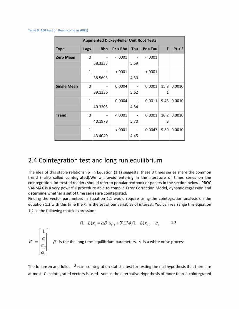
Table 9: ADF test on Realincome as AR(1)



Zero Mean 0 -

38.3333

<.0001 -

5.59

<.0001

1 -

38.5693

<.0001 -

4.30

<.0001

Single Mean 0 -

39.1336

0.0004 -

5.62

0.0001 15.8

1

0.0010

1 -

40.3303

0.0004 -

4.34

0.0011 9.43 0.0010

Trend 0 -

40.1978

<.0001 -

5.70

0.0001 16.2

3

0.0010

1 -

43.4049

<.0001 -

4.45

0.0047 9.89 0.0010

2.4 Cointegration test and long run equilibrium The idea of this stable relationship in Equation (1.1) suggests these 3 times series share the common trend ( also called cointegrated).We will avoid entering in the literature of times series on the cointegration. Interested readers should refer to popular textbook or papers in the section below.. PROC VARMAX is a very powerful procedure able to compile Error Correction Model, dynamic regression and determine whether a set of time series are cointegrated. Finding the vector parameters in Equation 1.1 would require using the cointegration analysis on the

equation 1.2 with this time the tx is the set of our variables of interest. You can rearrange this equation

1.2 as the following matrix expression :

titi

pitt xLxxL

)1()1( 101 1.3

t

i

y

t

1

t is the the long term equilibrium parameters. is a white noise process.

The Johansen and Julius trace cointegration statistic test for testing the null hypothesis that there are

at most r cointegrated vectors is used versus the alternative Hypothesis of more than r cointegrated

vectors or Eigenvalues or Characteristic roots are chosen over the mere test of another Augmented Dickey Fuller(ADF) test on the residuals .The VARMAX procedure tells that Rank=2 ( there is two cointegration vectors ) M1 (M2 )Money demand are cointegrated with the real income and the expected inflation because the trace value is smaller than the critical value at 5% level.

trace Tir1

k

log1 i #

1.4

proc varmax data=sasuser.Money_demand;

model M2Balance Realincome

E_inflation/cointtest=(johansen=(normalize=M2Balance));

run;

proc varmax data=sasuser.Money_demand;

model M1Balance Realincome

E_inflation/cointtest=(johansen=(normalize=M1Balance));

run;

Table 10: Johansen Cointegration test : Money demand(M2)

Cointegration Rank Test Using Trace Under Restriction

H0:

Rank=r

H1:

Rank>r Eigenvalue Trace

5%

Critical

Value

Drift in

ECM

Drift in

Process

0 0 0.4456 58.103

0

34.80 Constan

t

Constan

t

1 1 0.3838 30.377

2

19.99

2 2 0.1496 7.6189 9.13

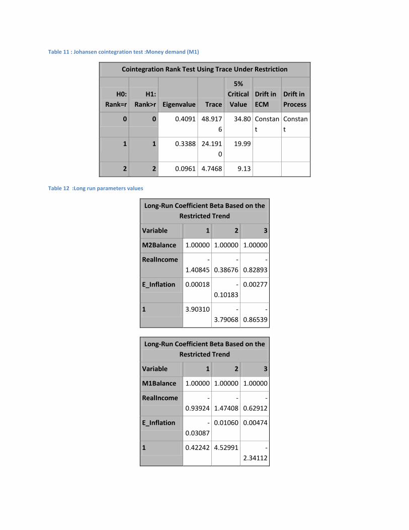
Table 11 : Johansen cointegration test :Money demand (M1)

Cointegration Rank Test Using Trace Under Restriction

H0:

Rank=r

H1:

Rank>r Eigenvalue Trace

5%

Critical

Value

Drift in

ECM

Drift in

Process

0 0 0.4091 48.917

6

34.80 Constan

t

Constan

t

1 1 0.3388 24.191

0

19.99

2 2 0.0961 4.7468 9.13

Table 12 :Long run parameters values

Long-Run Coefficient Beta Based on the

Restricted Trend

Variable 1 2 3

M2Balance 1.00000 1.00000 1.00000

RealIncome -

1.40845

-

0.38676

-

0.82893

E_Inflation 0.00018 -

0.10183

0.00277

1 3.90310 -

3.79068

-

0.86539

Long-Run Coefficient Beta Based on the

Restricted Trend

Variable 1 2 3

M1Balance 1.00000 1.00000 1.00000

RealIncome -

0.93924

-

1.47408

-

0.62912

E_Inflation -

0.03087

0.01060 0.00474

1 0.42242 4.52991 -

2.34112

3. Conclusion

The use of PROC ARIMA to study the stationary properties of money demand(M1 and M2),Real income and Expected inflation along with PROC VARMAX to investigate the cointegration relationship(common trend) of these variables for the case of Cote D’Ivoire suggests the stability of both M1 and M2 in the long run .All the variables appear to have the same order of integration of order 1( AR(1) processes with drift) .Finally It should be noted that the cointegration regression helps understand the long -run relationship of the money demand and its components but provides little answer when it comes to examine the short-run dynamics of the money demand. A method such as the Error Correction Model (ECM) method developed by Engle and Granger eloquently allows us to analyze the short-run deviation of the real money demand from its expected long-run path.

4- References

Bahmani-Oskooee, M., & Gelan, A. (2009). How stable is the demand for money in African countries? Journal of Economic Studies, 36(3), 216--235.

Drama, B. G. H., & Yao, S. (2010). The Demand for Money in Cote dâ€Ivoire: Evidence from the

Cointegration Test. University Library of Munich, Germany. Retrieved from http://ideas.repec.org/p/pra/mprapa/20131.html

Fielding, D., & Shields, K. (2001). Modelling macroeconomic shocks in the CFA Franc Zone. Journal of

Development Economics, Journal of Development Economics, 66(1), 199-223. Friedman, M. (1956) `The quantity theory of money- a restatement' in: Studies in the quantity theory of

money, M.Friedman (Ed.), Chicago, IL: University of Chicago Press

Robert A. Yaffee and Monnie McGee. An Introduction to Time Series Analysis and Forecasting: with Applications of SAS and SPSS

William Greene. Econometric Analysis, Fifth Edition.

Contact information:

Your comments and questions are valued and encouraged. Please contact the author at : Gerard G Tano Faner Hall 4th floor room 4041 1000 Faner Drive Mail Code 4515 Southern Illinois University Carbondale Carbondale, IL 62901-4515, U.S.A. Email:[email protected] Phone : (618) 453-5078

http://ideas.repec.org/p/pra/mprapa/20131.html

Trademark information

SAS and all other SAS Institute Inc. product or service names are registered trademarks or trademarks of SAS Institute Inc. in the USA and other countries. ® indicates USA registration. Other brand and product names are trademarks of their respective companies.