monetarypolicyinadata-richenvironment -...

Journal of Monetary Economics 50 (2003) 525–546

Monetary policy in a data-rich environment$

Ben S. Bernankea,*, Jean Boivinb

aDepartment of Economics, Princeton University, Princeton, NJ 08544, USAbGraduate School of Business, Columbia University, New York, NY 10027, USA

Received 1 August 2000; accepted 9 September 2002

Abstract

Most empirical analyses of monetary policy have been confined to frameworks in which the

Federal Reserve is implicitly assumed to exploit only a limited amount of information, despite

the fact that the Fed actively monitors literally thousands of economic time series. This article

explores the feasibility of incorporating richer information sets into the analysis, both positive

and normative, of Fed policymaking. We employ a factor-model approach, developed by

Stock, J.H., Watson, M.W., Diffusion Indices, Journal of Business & Economic Statistics

2002, 20 (2) 147, Forecasting Inflation, 1999, Journal of Monetary Economics 44 (2) 293, that

permits the systematic information in large data sets to be summarized by relatively few

estimated factors. With this framework, we reconfirm Stock and Watson’s result that the use

of large data sets can improve forecast accuracy, and we show that this result does not seem to

depend on the use of finally revised (as opposed to ‘‘real-time’’) data. We estimate policy

reaction functions for the Fed that take into account its data-rich environment and provide a

test of the hypothesis that Fed actions are explained solely by its forecasts of inflation and real

activity. Finally, we explore the possibility of developing an ‘‘expert system’’ that could

aggregate diverse information and provide benchmark policy settings.

r 2003 Elsevier Science B.V. All rights reserved.

JEL classification: E5

Keywords: Monetary policy

$Prepared for a conference on ‘‘Monetary Policy Under Incomplete Information’’, Gerzensee,

Switzerland, October 12–14, 2000. Min Wei and Peter Bondarenko provided able research assistance. We

thank Mark Watson and our discussants, Ignazio Angeloni and Harald Uhlig, for helpful comments, and

Dean Croushore for assistance with the Greenbook data. This research was funded in part by NSF grant

SES-0001751.

*Corresponding author. Tel.: +1-609-258-5635; fax: +1-609-258-5533.

E-mail address: [email protected] (B.S. Bernanke).

0304-3932/03/$ - see front matter r 2003 Elsevier Science B.V. All rights reserved.

doi:10.1016/S0304-3932(03)00024-2

1. Introduction

Monetary policy-makers are inundated by economic data. Research departmentsthroughout the Federal Reserve System, as in other central banks, monitor andanalyze literally thousands of data series from disparate sources, including data at awide range of frequencies and levels of aggregation, with and without seasonal andother adjustments, and in preliminary, revised, and ‘‘finally revised’’ versions. Nor isexhaustive data analysis performed only by professionals employed in part for thatpurpose; observers of Alan Greenspan’s chairmanship, for example, haveemphasized his own meticulous attention to a wide variety of data series (Beckner,1996).The very fact that central banks bear the costs of analyzing a wide range of data

series suggests that policy-makers view these activities as relevant to their decisions.Indeed, recent econometric analyses have confirmed the longstanding view ofprofessional forecasters, that the use of large number of data series may significantlyimprove forecasts of key macroeconomic variables (Stock and Watson, 1999, 2002;Watson, 2000). Central bankers’ reputations as data fiends may also reflectmotivations other than minimizing average forecast errors, including multiple andshifting policy objectives, uncertainty about the correct model of the economy, andthe central bank’s political need to demonstrate that it is taking all potentiallyrelevant factors into account.1

Despite this reality of central bank practice, most empirical analyses of monetarypolicy have been confined to frameworks in which the Fed is implicitly assumed toexploit only a limited amount of information. For example, the well-known vectorautoregression (VAR) methodology, used in many recent attempts to characterizethe determinants and effects of monetary policy, generally limits the analysis to eightmacroeconomic time series or fewer.2 Small models have many advantages,including most obviously simplicity and tractability. However, we believe that thisdivide between central bank practice and most formal models of the Fed reflects atleast in part researchers’ difficulties in capturing the central banker’s approach todata analysis, which typically mixes the use of large macroeconometric models,smaller statistical models (such as VARs), heuristic and judgmental analyses, andinformal weighting of information from diverse sources. This disconnect betweencentral bank practice and academic analysis has, potentially, several costs: First, byignoring an important dimension of central bank behavior and the policyenvironment, econometric modeling and evaluation of central bank policies maybe less accurate and informative than it otherwise would be. Second, researchers maybe foregoing the opportunity to help central bankers use their extensive data sets to

1A related motivation, consistent with the approach of our paper, is that the Fed thinks of concepts like

‘‘economic activity’’ as being latent variables in a large system. Such a viewpoint would be consistent with

classical Burns and Mitchell business cycle analysis. See also the latent variable approach to business cycle

modeling of Stock and Watson (1989).2See Christiano et al. (2000) for a survey of the monetary VAR literature. Leeper et al. (1996) are able to

increase the number of variables analyzed through the use of Bayesian priors, but their VAR systems still

typically contain fewer than 20 variables.

B.S. Bernanke, J. Boivin / Journal of Monetary Economics 50 (2003) 525–546526

improve their forecasting and policymaking. It thus seems worthwhile for analysts totry to take into account the fact that in practice monetary policy is made in a ‘‘data-rich environment’’.This paper is an exploratory study of the feasibility of incorporating richer

information sets into the analysis, both positive and normative, of Federal Reservepolicy-making. Methodologically, we are motivated by the aforementioned work ofStock and Watson. Following earlier work on dynamic factor models,3 Stock andWatson have developed dimension reduction schemes, akin to traditional principalcomponents analysis, that extract key forecasting information from ‘‘large’’ data sets(i.e., data sets for which the number of data series may approach or exceed thenumber of observations per series). They show, in simulated forecasting exercises,that their methods offer potentially large improvements in the forecasts ofmacroeconomic time series, such as inflation. From our perspective, the Stock–Watson methodology has several additional advantages: First, it is flexible, in thesense that it can potentially accommodate data of different vintages, at differentfrequencies, and of different spans, thus replicating the use of multiple data sourcesby central banks. Second, their methodology offers a data-analytic framework that isclearly specified and statistically rigorous but remains agnostic about the structure ofthe economy. Finally, although we do not take advantage of this feature here, theirmethod can be combined with more structural approaches to improve forecastingstill further (Stock and Watson, 1999).The rest of our paper is structured as follows. Section 2 extends the research of

Stock and Watson by further investigating the value of their methods in forecastingmeasures of inflation and real activity (and, by extension, the value of those forecastsas proxies for central bank expectations). We consider three alternative data sets:first, a ‘‘real-time’’ data set, in which the data correspond closely to what wasactually observable by the Fed when it made its forecasts; second, a data setcontaining the same time series as the first but including only finally revised data; andthird, a much larger, and revised, data set based on that employed by Stock andWatson (2002). We compare forecasts from these three data sets with each other andwith historical Federal Reserve forecasts, as reported in the Greenbook. We find, inbrief, that the scope of the data set (the number and variety of series included)matters very much for forecasting performance, while the use of revised (as opposedto real-time) data seems to matter much less. We also find that ‘‘combination’’forecasts, which give equal weight to our statistical forecasts and Greenbookforecasts, can sometimes outperform Greenbook forecasts alone.In Section 3 we apply the Stock–Watson methodology to conduct a positive

analysis of Federal Reserve behavior. Specifically, we estimate monetary policyreaction functions, or PRFs, which relate the Fed’s instrument (in this article, the fedfunds rate) to the state of the economy, as determined by the full information set.Our interest is in testing formally whether the Fed’s reactions to the state of the

3Sargent and Sims (1977) is an important early reference. See also Quah and Sargent (1993), Forni and

Reichlin (1996), and Forni et al. (2000) for related approaches. Knox et al. (2000) describes a related

shrinkage estimator.

B.S. Bernanke, J. Boivin / Journal of Monetary Economics 50 (2003) 525–546 527

economy can be accurately summarized by a forward-looking Taylor rule of the sortstudied by Battini and Haldane (1999) and Clarida et al. (1999, 2000), among others;or whether, as is sometimes alleged, the Fed responds to variables other thanexpected real activity and expected inflation. We show here that application of theStock–Watson methodology to this problem provides both a natural specificationtest for the standard forward-looking PRF, as well as a nonparametric method forstudying sources of misspecification.Section 4 briefly considers whether the methods employed in this paper might not

eventually prove useful to the Fed in actual policy-making. In particular, one canimagine an ‘‘expert system’’ that receives data in real time and provides a consistentbenchmark estimate of the implied policy setting. To assess this possibility, weconduct a counterfactual historical exercise, in which we ask how well monetarypolicy would have done if it had relied mechanically on SW forecasts and somesimple policy reaction functions. Perhaps not surprisingly, though our expert systemperforms creditably, it does not match the record of human policy-makers.Nevertheless, the exercise provides some interesting results, including the findingthat the inclusion of estimated factors in dynamic models of monetary policy canmitigate the well-known ‘‘price puzzle’’, the common finding that changes inmonetary policy seem to have perverse effects on inflation. Section 5 concludes bydiscussing possible extensions of this research.

2. Forecasting in a data-rich environment: some further results

Stock and Watson (1999a, b), henceforth SW, have shown that dynamic factormethods applied to large data sets can lead to improved forecasts of keymacroeconomic variables, at least in simulated forecasting exercises. In this sectionwe investigate three issues relevant to the applications we have in mind. First, weseek to determine whether the SW results are sensitive to the use of ‘‘real-time’’,rather than finally revised data. Second, we ask whether data sets containing manytime series forecast appreciably better than data sets with fewer series. Finally, wecompare simulated forecasts using SW methods applied to alternative data sets tohistorical Fed forecasts, as published in the Greenbook.We first briefly review the SW method and our implementation of it. Following

SW (2002), to which the reader is referred for details, we assume that at date t theforecaster has available a large number of time series, collectively denoted Xt: Again,by ‘‘large’’ we mean to allow for the possibility that the number of time seriesapproaches or even exceeds the number of observations per series. Let wt be a scalartime series, say inflation, which we would like to forecast. Both Xt and wt aretransformed to be stationary, and for notational simplicity we assume also that eachseries is mean-zero. Assume that ðXt;wtþ1Þ have an approximate dynamic factormodel representation:

Xt ¼ LFt þ et;

wtþ1 ¼ bFt þ etþ1:ð1Þ


In (1) the Ft are (a relatively small number of) unobserved factors that summarizethe systematic information in the data set. L is the factor-loading matrix, and b is arow-vector of parameters that relates the variable to be forecasted to the currentrealizations of the factors.4 In a macroeconomic context (1) might be motivated bystandard dynamic general equilibrium models of the economy, in which the reducedform expressions for the exogenous and endogenous variables are linear combina-tions of a few fundamental shocks (the factors). Note that Ft may contain laggedvalues of the underlying factors; this is the sense in which this model is ‘‘dynamic’’.The idiosyncratic error terms et may be weakly correlated, in a sense described bySW. We assume Eðetþ1 Ftj Þ ¼ 0:SW (2002) show that the factors in a model of the form (1) can be consistently

estimated by principal components analysis, when the time series dimension (T) andthe cross-section dimension (N) both go to infinity. The estimated factor model (1)can then be used in the obvious way to forecast the series wt: We note, though, thatthe efficiency properties of the SW estimator are still unknown, so that this approachoffers no guidance on how optimally to weight variables Xt for estimation andforecasting. This is an important topic for future research.A useful feature of the SW framework, as implemented by an EM algorithm, is

that it permits one to deal systematically with data irregularities (SW, 2002,Appendix A). In particular, our implementation of the SW approach allows thecollection of time series X to include both monthly and quarterly series, series thatare introduced mid-sample or are discontinued, and series with missing values. Thefact that at each date the Fed may be looking at a different vintage (revision) of agiven underlying data series is also incorporated automatically in our implementa-tion.In the next section we consider forward-looking policy reaction functions under

which the Fed is assumed to respond to its forecasts of inflation and real activity.Accordingly, we focus in this section on forecasting CPI inflation and two measuresof economic activity, the unemployment rate and industrial production. Theprincipal results reported below are based on three alternative data sets: a ‘‘real-time’’ data set, a data set containing the same variables as the first but in finallyrevised form, and the finally revised data set employed by SW (2002). We describeeach of these data sets very briefly; for more details, see the on-line appendixavailable at http://www.columbia.edu/Bjb903 or in the working-paper version ofthis article.

2.1. Real-time data set

A realistic description of Fed behavior requires recognition not only of the centralbank’s data-rich environment, as we have emphasized so far, but also of the fact thatthe Fed observes the economy in ‘‘real time’’. That is, the economic data actually

4Although we have not allowed explicitly for time variation in the parameters, SW (2002) show that,

even in the presence of modest parameter drift or large jumps caused by data irregularities, the factors are

consistently estimated by the principal component procedure used in this paper.


http://www.columbia.edu/jb903

available to the Fed in a particular month may differ significantly from the finallyrevised version of the same data, available only for retrospective analysis. Indeed,recent research has shown that the common practice of using finally revised ratherthan real-time data in empirical studies is often not innocuous. For example,Orphanides (2001) shows that the description of the historical conduct of monetarypolicy provided by a standard Taylor rule is much less convincing when estimatedusing real-time data.To get a sense of the importance of this issue in our context, we created a

composite real-time data set, consisting of the union of the real-time data setsconstructed by Croushore and Stark (2002) and by Ghysels et al. (1998), with modestupdating.5 These two data sets include series on GDP and its components, aggregateprice measures, and monetary aggregates and components. To these we added avariety of financial indicators (stock price indices, interest rates, and exchange rates),which can safely be assumed both to be known immediately and not to be revised.Finally, as the CPI and PPI are rarely revised, except for rebasing when the base yearis changed, we included sub-components of these two indices in the data set.6 Thecomplete real-time data set used here includes 78 data series, of both monthly andquarterly frequency. We include data from January 1959 onward if available,otherwise from the earliest date available for each series.

2.2. Fully revised data set

To determine the importance of the real-time nature of our first data set, we alsoreplicated all our results using what we call, loosely, the ‘‘fully revised’’ data set. Thefully revised data set consists of the identical data series as the real-time data set,except that data revisions known as of the last period of our sample, 1998:12, areincorporated. Note that, in both this database and the one described next, weadopted timing conventions consistent with the real-time database. For example,unlike SW, who assume that the CPI for February is known when the Februaryinflation forecasts are constructed, we incorporate the 1-month lag found in real-time data and assume that only the CPI through January is known when theFebruary forecast is made. Similarly, the value of fourth-quarter GDP is assumednot to be known until February, first-quarter GDP is not assumed known until May,and so on.

2.3. Stock–Watson data set

Databases differ not only in whether they include real-time or revised data, butalso in their breadth of coverage. Unfortunately, our real-time data set is necessarilysomewhat limited both in the number and scope of the time series included. Ifforecasts constructed with this data set are poor, we would like to know whether the

5We thank these authors for graciously providing us with their data.6Our results were robust to excluding the CPI and PPI components and to various alternative

assumptions about the timing of information.


problem is the SW method or simply the limited information in the database. Toisolate this factor, we reproduced all our forecasting results using the unbalanced,large (215 variables), and revised database used by SW (2002). The SW data wereoriginally obtained from the DRI-McGraw Hill Basic Economics database.

2.4. Forecasting results

For each of the three data sets, we conducted simulated estimation and forecastingexercises for CPI inflation, industrial production, and the unemployment rate, atboth 6- and 12-month horizons. Recursive forecasts were made from the perspectiveof each month from January 1970 to December 1998, using only the data that (inprinciple at least) would have been available at each date. More specifically, webegan by re-estimating the SW model for each month from January 1970 on,assuming three distinct factors per period.7 Following SW, we then constructedforecasts of each variable using: (1) the estimated factors plus autoregressive terms inthe forecasted variable (these forecasts are designated FM-AR), (2) the estimatedfactors augmented by VAR terms in inflation, industrial production, unemployment,and the federal funds rate (FM-VAR), (3) a purely autoregressive model in theforecasted variable (AR); and (4) the vector autoregressive terms in inflation, realactivity, and the federal funds rate only (VAR). For each period’s estimation, theSchwartz information criterion (BIC) was used to determine the number of lags ofthe factors (between 0 and 3) and of the additional variables (between 1 and 6)included in the forecasting equation. Lagged variables used in the forecasting modelswere in all cases taken from the real-time data set, so that any differences in forecastsarise solely from differences in the estimated factors, not the auxiliary forecastingvariables. The root mean square error (RMSE) of forecasts was constructed bycomparing model forecasts to the finally revised data.Table 1 shows the results. For each variable to be forecasted, entries in the table

show the mean square error of forecast relative to that of the forecast from a baselineautoregressive model (with no factors). Of the two numbers given in each entry, thefirst refers to the 6-month horizon and the second to the 12-month horizon. Theabsolute RMSEs for the AR model are reported below each portion of the table. Theresults suggest three conclusions.First, for the real-time data set, the forecasting performance of the factor model is

moderately disappointing. For CPI inflation, the forecasts that include estimatedfactors do no better than a simple AR model. On the other hand, the FM-AR modelon real-time data performs about 10–15% better than the AR model for industrialproduction and 15–20% better than the AR model for unemployment.

7Note that instead of fixing the number of factors to three, we could have used the information criterion

proposed by Bai and Ng (2002) to determine the number of factors in our data set. Experimentation with

this criterion gave the result that the number of factors in the data set was quite large (greater than 12).

This might not be surprising, however, since this is a static criterion, which implies that two lags of a given

factor would be counted as two different factors. In any case, the following results were not significantly

changed if the number of factors used was between 3 and 6.


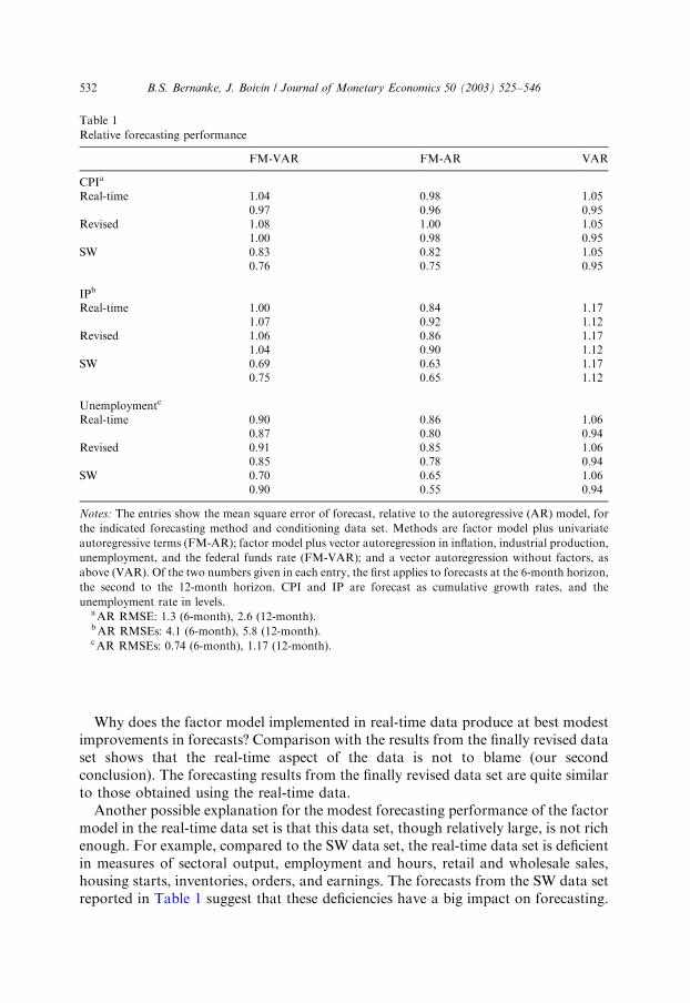
Why does the factor model implemented in real-time data produce at best modestimprovements in forecasts? Comparison with the results from the finally revised dataset shows that the real-time aspect of the data is not to blame (our secondconclusion). The forecasting results from the finally revised data set are quite similarto those obtained using the real-time data.Another possible explanation for the modest forecasting performance of the factor

model in the real-time data set is that this data set, though relatively large, is not richenough. For example, compared to the SW data set, the real-time data set is deficientin measures of sectoral output, employment and hours, retail and wholesale sales,housing starts, inventories, orders, and earnings. The forecasts from the SW data setreported in Table 1 suggest that these deficiencies have a big impact on forecasting.

Table 1

Relative forecasting performance

FM-VAR FM-AR VAR

CPIa

Real-time 1.04 0.98 1.050.97 0.96 0.95

Revised 1.08 1.00 1.051.00 0.98 0.95

SW 0.83 0.82 1.050.76 0.75 0.95

IPb

Real-time 1.00 0.84 1.171.07 0.92 1.12

Revised 1.06 0.86 1.171.04 0.90 1.12

SW 0.69 0.63 1.170.75 0.65 1.12

Unemploymentc

Real-time 0.90 0.86 1.060.87 0.80 0.94

Revised 0.91 0.85 1.060.85 0.78 0.94

SW 0.70 0.65 1.060.90 0.55 0.94

Notes: The entries show the mean square error of forecast, relative to the autoregressive (AR) model, for

the indicated forecasting method and conditioning data set. Methods are factor model plus univariate

autoregressive terms (FM-AR); factor model plus vector autoregression in inflation, industrial production,

unemployment, and the federal funds rate (FM-VAR); and a vector autoregression without factors, as

above (VAR). Of the two numbers given in each entry, the first applies to forecasts at the 6-month horizon,

the second to the 12-month horizon. CPI and IP are forecast as cumulative growth rates, and the

unemployment rate in levels.aAR RMSE: 1.3 (6-month), 2.6 (12-month).bAR RMSEs: 4.1 (6-month), 5.8 (12-month).cAR RMSEs: 0.74 (6-month), 1.17 (12-month).


Using the estimated SW factors in the construction of the forecasts significantlyreduces forecast errors, relative to the AR benchmark, in all cases. In particular, theRMSE of forecast is as much as a quarter lower for inflation, and as much as a thirdlower for industrial production or unemployment. Hence our third conclusion, thatrelevant information for forecasting may exist in a wide variety of variables.Although these results are to some degree mixed, we take them as generally

supportive of the SW approach. First, we have seen that the use of finally revised (asopposed to real-time) data is probably not responsible for the good forecastingperformance reported by Stock and Watson (1999, 2002), at least for the data usedhere. Second, we have seen that forecasting performance improves significantly whenthe conditioning data set contains a wide variety of macroeconomic time series,supporting results in Watson (2000).8 The results are likewise consistent with thepremise of this paper, that taking account of the data-rich environment of monetarypolicy may be important in practice.Another question of interest is whether SW methods might be of use to the

Federal Reserve itself. The Federal Reserve already makes regular forecasts, basedon a wide range of information. These forecasts are circulated to policymakers aspart of the Greenbook briefing and reported, with a 5-year lag, to the general public.Romer and Romer (2000) have documented that Greenbook forecasts areexceptionally accurate compared to for-profit private-sector forecasts, suggestingthat the Fed has private information, special expertise, or both.9

Table 2 compares the accuracy of Greenbook forecasts to forecasts for inflationand unemployment obtained by the same methods as described above. We considerfactor models augmented by both AR and VAR methods and present results basedon both the real-time data sets and the SW data set. (Results from the revised dataset are similar to those from the real-time data set and hence are omitted.) As it iswell known that averages of forecasts are often superior to the components of theaverage, we also consider ‘‘combination’’ forecasts, that give 50% weight to the FM-AR or FM-VAR forecast and 50% weight to the Greenbook forecast (third andfourth columns of Table 2). Consistent with the structure of Greenbook forecasts,four RMSEs of forecast are shown in each cell. The top RMSE pertains to theforecast for the first complete quarter after the month of forecast, the secondpertains to the forecast for the second complete quarter following the month offorecast, and so on. Forecast errors are calculated only for months in which newGreenbook forecasts are issued (i.e., months of FOMC meetings). So for example, ifa meeting is held in January the Greenbook includes forecasts for the second quarterof the year (April–June), the third quarter, the fourth quarter, and the first quarter of

8As Chris Sims pointed out to us, further improvements in forecasts might be achieved by imposing

Bayesian priors in estimation of the forecasting models.9 In contrast to our unconditional forecasts, the Greenbook forecasts are conditional on a given policy

scenario (generally of no change in the policy stance). As a result, a comparison of the two set of forecasts

might be biased. Note that the same caveat applies to the Romer and Romer (2000) exercise.


the next year.10 The comparisons between the Greenbook and other forecasts take accountof this timing structure. The sample period is 1981:01–1995:12 for CPI inflation and1970:1–1995:12 for unemployment, coinciding with the availability of Greenbook forecasts.Generally, as might be anticipated, Table 2 shows Greenbook forecasts to be more

accurate than SW forecasts, which in turn are more accurate than forecasts based on

Table 2

Comparison with Greenbook forecasts

FM-VAR FM-AR Greenbook

and FM-VAR

Greenbook

and FM-AR

Greenbook

CPI

Real-time 2.641 3.262 2.516 2.789

3.100 3.721 2.701 3.014

2.803 3.512 2.467 2.766

3.114 3.607 2.664 2.816

SW 2.547 3.400 2.377 2.836

2.835 3.424 2.530 2.809

2.772 3.108 2.430 2.494

2.979 3.331 2.521 2.665

Greenbook 2.770

2.705

2.426

2.554

Unemployment

Real-time 0.528 0.531 0.446 0.448

0.763 0.784 0.635 0.648

0.999 0.996 0.797 0.813

1.155 1.169 0.907 0.933

SW 0.490 0.440 0.441 0.420

0.690 0.637 0.623 0.605

0.855 0.794 0.757 0.748

0.963 0.890 0.853 0.844

Greenbook 0.455

0.642

0.789

0.897

Notes: The entries show the RMSE of forecast, in percentage points, for CPI inflation, annualized, and for

the unemployment rate, in percentage points. Results are for months in which a new Greenbook forecast

was issued only. The first entry in each box pertains to the first full calendar quarter subsequent to the

month of forecast, the second entry to the second full calendar quarter, and so on. For the real-time and

SW data sets, forecasts are calculated alternatively by the factor model plus univariate autoregressive

terms (FM-AR), or by factor model plus vector autoregression in inflation, output, and the federal funds

rate (FM-VAR). Greenbook forecasts are the actual real-time forecasts made by the Federal Reserve.

Combination forecasts give 50% weight each to the statistical model and the Greenbook forecast. The

sample period is 1981:01–1995:12 for CPI-inflation and 1970:01–1995:12 for unemployment, coinciding

with the availability of Greenbook forecasts.

10Notice that the precise horizon of the forecast depends on whether the FOMC meeting is in the first,

second, or third month of a quarter. We broke down the results by month of quarter and found that they

were similar to the results reported in Table 2.


the real-time data set. However, the magnitudes of the differences are not large.Indeed, the FM-VAR model in both the real-time and SW data sets does marginallybetter than the Greenbook at forecasting next quarter’s inflation, and for longerhorizons their disadvantage is small. The unemployment forecasts are also generallycomparable. These results are interesting, given that Romer and Romer (2000, Table5) find that the Greenbook outperforms private forecasters significantly in inflationforecasting (albeit for inflation measured by the GDP deflator rather than the CPI).The results from the combination forecasts are even more impressive. Particularly

for unemployment, these weighted-average forecasts seem to do as well or betterthan the Greenbook at all horizons. Overall, we take the results as providing someevidence that factor-model methods could help the Fed forecast inflation andunemployment.11 An additional advantage of the SW methods is that are statisticallywell grounded and replicable, as opposed to the ‘‘black box’’ of the Greenbook.

3. Estimating the Fed’s policy reaction function in a data-rich environment

In this section we apply the Stock–Watson methodology to a positive analysis ofFederal Reserve behavior. We model the Fed’s behavior by a policy reactionfunction (PRF), under which a policy instrument is set in response to the state of theeconomy, as measured by the estimated factors.The standard practice in much recent empirical work has been to use tightly

specified PRFs, such as the so-called Taylor rule (Taylor, 1993). According to thebasic Taylor rule, the Fed moves the fed funds rate (Rt) in response to deviations ofinflation from target (pt) and of output from potential (yt):

Rt ¼ f0 þ fppt þ fyyt þ et: ð2Þ

Variants of this rule have been considered in which the output gap is replaced byother real activity measures—such as unemployment—and in which lags of the fundsrate are included to allow for interest-rate smoothing.More recently, some papers (Battini and Haldane, 1999; Clarida et al., 1999, 2000)

have studied rules in the general form of (2) in which the Fed is assumed to respondto forecasts of inflation and real activity. These forward-looking specificationsappear to fit well, and they are appealing because they recognize the Fed’s need toincorporate policy lags into its decisions. Specifically, these studies have estimatedPRFs of the form:

Rt ¼ f0 þ fp #ptþh1jt þ fy #ytþh2jt þ et; ð3Þ

where hatted variables indicate expectations, t is the date at which the forecast isbeing made and h1 and h2 are respectively the lengths of the forecast horizon forinflation and real activity.

11Our discussant Harald Uhlig also noted that the SW forecasting approach could be used to obtain

better estimates in real time of the current value of variables known to be subject to large revisions, such as

GDP.


A variety of methods have been used to estimate these ‘‘forward-looking’’ PRFs(see, e.g., Clarida et al., 1999, 2000, for discussions). Here we estimate PRFsanalogous to (3) under the assumption that the Fed uses information from manymacroeconomic time series, i.e., a situation in which the dimension of Xt is large. Fortractability, we assume as before that Xt obeys an approximate dynamic factormodel such as (1), with the factors given by Ft:Assuming that the PRF is linear and (for the moment) the factors are known, and

assuming that the state of the economy is summarized by the factors, we can write areduced-form expression for the policy reaction function as

Rt ¼ aFt þ et; ð4Þ

where a is a row vector. Absent any restrictions on a; Eq. (4) constitutes a fairlyflexible specification of the PRF. For example, it does not preclude a direct policyresponse to a variety of factors, such as (for example) a ‘‘financial market factor.’’12

Eq. (4) is also consistent with the specification of the forward-looking Taylor rule,Eq. (3); in this case the response of policy to the factors derives solely from theirforecasting power for inflation and real activity. To illustrate, suppose we had aknown forecasting model based on the factors. Then forecasts would be given by

#ptþh1jt ¼ gpt Fpt ;

#ytþh2jt ¼ gyt F

yt ;

ð5Þ

where Fpt and F

yt are subsets of Ft and the g’s are conformable row vectors.

Substituting (5) into (3) we get the following reduced-form expression for theforward-looking Taylor rule:

Rt ¼ f0 þ fpgpt Fpt þ fygy

t Fyt þ et; ð6Þ

Comparing expressions (6) and (3) we see that the restrictions imposed by theforward-looking Taylor rule specification can be precisely identified. If the factorsand the forecasting model were known, it would thus be possible to test if this Taylorrule specification accurately describes Fed behavior, and if not, to determine to whatother information the Fed is responding.However, the factors Ft are of course not observed in practice and need to be

estimated. The forecasting model required to obtain #ptþh1jt and #ytþh2jt is alsounknown; that is, the parameters gp and gy must be estimated. Further, since wewant to think of the Fed as continuously updating its knowledge of the economy,i.e., as simultaneously re-estimating the forecasting models and estimating thefactors as new data become available, the relationship between (6) and (3) is morecomplicated than the previous paragraph suggests. In fact, a PRF like (6) cannot beestimated directly if the factors are estimated recursively, and there are no simplerestrictions relating the parameters of (6) to those of (3). The reason is that while thefirst element of #FtjT must correspond to the first element of #FsjT for any s and t, since

12Eq. (4) does preclude the possibility that policy responds to the idiosyncratic error terms et: However,this restriction is inessential, as the equation can be modified in a straightforward way to include

additional regressors, possibly including lags of the dependent variable. We include lags of the federal

funds rate in the PRFs estimated below.


both are obtained simultaneously from the same information set, there is nothing inthe recursive estimation guaranteeing that the first element of #Ftjt corresponds to thefirst element of #Fsjs:It is however still possible to test the Taylor rule restrictions implicit in Eq. (3). To

do so, at each period we compute the fitted values of the policy instrument, #Rtþ1jt;obtained from estimating

Rt ¼ at#FtjT þ ut ð7Þ

over the period [1,T]. Computed in this fashion, #Rtjt is comparable to #ptþh1jt and#ytþh2jt; in particular it is independent of the normalization of the factors. Thestructure imposed by (6) can thus be tested by determining if #Rtjt appearssignificantly, i.e. by estimating

Rt ¼ f0 þ fp #ptþh1jt þ fy #ytþh2jt þ Z #Rtjt þ et ð8Þ

and testing if Z ¼ 0:13 We call Z #Rtjt the excess policy response. In addition, if thespecification (6) is rejected, the portion of the excess policy response that isorthogonal to the other regressors in (8) becomes a potentially useful diagnosticvariable. Specifically, the correlation of the orthogonal excess policy response withthe variables in the conditioning data set provides information on which variables, ortypes of variables, have been incorrectly omitted from the PRF.Table 3 presents estimated policy reaction functions for the Fed. The first part of

Table 3 reports a PRF with only forecasted 12-month ahead inflation on the right-hand side, and no measure of real activity. The second part of the table adds, as ameasure of real activity, the difference between 6-month ahead forecastedunemployment and a 5-year moving average of unemployment, the latter proxyingfor the natural rate.The forecasts that enter the PRFs come from three alternative sources: FM-AR

estimates from the real-time data set and the SW data set, and from the Greenbook.The sample periods for the real-time data set and the SW data set are 1970:01–1998:12 (in addition, we allow 11 years of lagged data for estimation of the factors,as noted earlier). A fair amount of evidence supports the hypothesis of PRFinstability, e.g., Clarida et al. (1999, 2000) and Boivin (2001) all found that the Fed’sresponse to inflation was significantly higher in the post-Volcker era than before.Hence, in addition to full-sample results, we present results for the pre-Volcker (priorto October 1979) and post-Volcker disinflation (after 1982) subsamples. Dataavailability (specifically, the availability of CPI-inflation forecasts) restricts us to the1981–1995 sample period for the PRFs employing Greenbook forecasts. We alsoshow results with and without allowance for time variation in the estimated constantterm, modeled as a random walk parameter. Time variation in the constant isintended to proxy, among other things, for changes in the Fed’s inflation target or in

13 It is important to note that this specification test, and all statistical inference made on the estimated

PRF for that matter, is potentially contaminated by the presence of generated regressors. In our case

however, the required correction to the standard errors relies on the asymptotic distribution of the factors.

Authors’ calculations, based on Theorem 1 of Bai and Ng (2002), show that if N > T ; the factors can betreated as known. We are indebted to Mark Watson and Jushan Bai for suggesting this point.


Table 3

Estimated policy reaction functions

Data/sample Response toinflation

Response toreal activity measure

Significance of excesspolicy response

Measure of real activity: None

Real-time1970:01–1998:12 0.683 (0.001) * 0.003*1970:01–1979:10 0.822 (0.004) 0.0621983:01–1998:12 �0.271 (0.795) 0.000*

With TVP1970:01–1998:12 1.098 (0.000) 0.012*1970:01–1979:10 0.973 (0.002) 0.029*1983:01–1998:12 0.595 (0.769) 0.000*

SW1970:01–1998:12 0.804 (0.000) * 0.1961970:01–1979:10 0.776 (0.031) 0.9571983:01–1998:12 1.138 (0.137) 0.001*

With TVP1970:01–1998:12 1.223 (0.000) 0.1501970:01–1979:10 0.967 (0.010) 0.9161983:01–1998:12 1.552 (0.044) 0.001*

Greenbook1981:01–1995:12 2.280 (0.000) 0.517

With TVP1981:01–1995:12 1.771 (0.000) 0.573

Measure of real activity: Forecasted unemployment gap

Real-time1970:01–1998:12 0.729 (0.000) �0.805 (0.048) 0.008*1970:01–1979:10 0.609 (0.007) �1.232 (0.000) 0.013*1983:01–1998:12 �0.255 (0.786) �1.156 (0.354) 0.000*

With TVP1970:01–1998:12 1.101 (0.000) �1.192 (0.034) 0.013*1970:01–1979:10 1.040 (0.000) �1.105 (0.005) 0.002*1983:01–1998:12 0.389 (0.812) �2.105 (0.365) 0.000*

SW1970:01–1998:12 0.884 (0.000) �0.895 (0.068) 0.3371970:01–1979:10 0.628 (0.091) �1.079 (0.049) 0.5631983:01–1998:12 0.856 (0.291) �1.135 (0.264) 0.001*

With TVP1970:01–1998:12 1.278 (0.000) �1.239 (0.047) 0.2871970:01–1979:10 1.037 (0.012) �0.707 (0.181) 0.6281983:01–1998:12 1.335 (0.114) �1.174 (0.297) 0.002*


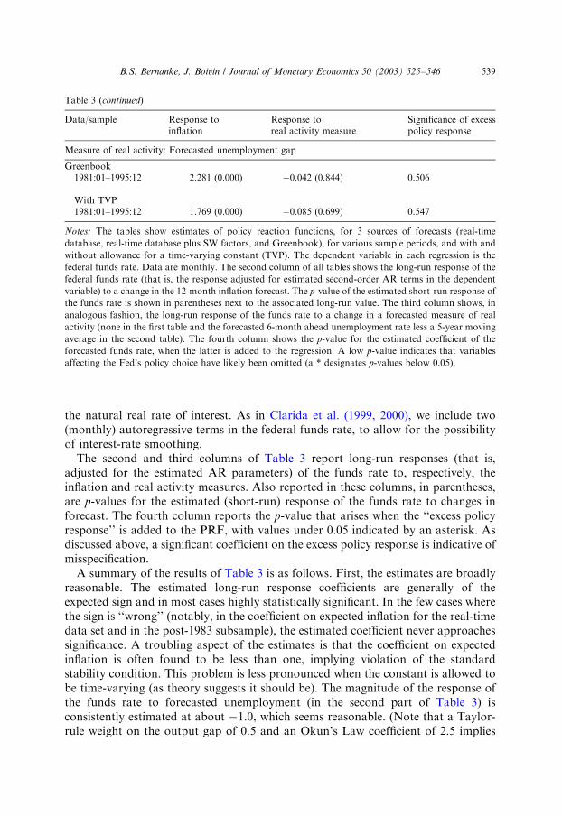
the natural real rate of interest. As in Clarida et al. (1999, 2000), we include two(monthly) autoregressive terms in the federal funds rate, to allow for the possibilityof interest-rate smoothing.The second and third columns of Table 3 report long-run responses (that is,

adjusted for the estimated AR parameters) of the funds rate to, respectively, theinflation and real activity measures. Also reported in these columns, in parentheses,are p-values for the estimated (short-run) response of the funds rate to changes inforecast. The fourth column reports the p-value that arises when the ‘‘excess policyresponse’’ is added to the PRF, with values under 0.05 indicated by an asterisk. Asdiscussed above, a significant coefficient on the excess policy response is indicative ofmisspecification.A summary of the results of Table 3 is as follows. First, the estimates are broadly

reasonable. The estimated long-run response coefficients are generally of theexpected sign and in most cases highly statistically significant. In the few cases wherethe sign is ‘‘wrong’’ (notably, in the coefficient on expected inflation for the real-timedata set and in the post-1983 subsample), the estimated coefficient never approachessignificance. A troubling aspect of the estimates is that the coefficient on expectedinflation is often found to be less than one, implying violation of the standardstability condition. This problem is less pronounced when the constant is allowed tobe time-varying (as theory suggests it should be). The magnitude of the response ofthe funds rate to forecasted unemployment (in the second part of Table 3) isconsistently estimated at about �1.0, which seems reasonable. (Note that a Taylor-rule weight on the output gap of 0.5 and an Okun’s Law coefficient of 2.5 implies

Greenbook1981:01–1995:12 2.281 (0.000) �0.042 (0.844) 0.506

With TVP1981:01–1995:12 1.769 (0.000) �0.085 (0.699) 0.547

Notes: The tables show estimates of policy reaction functions, for 3 sources of forecasts (real-time

database, real-time database plus SW factors, and Greenbook), for various sample periods, and with and

without allowance for a time-varying constant (TVP). The dependent variable in each regression is the

federal funds rate. Data are monthly. The second column of all tables shows the long-run response of the

federal funds rate (that is, the response adjusted for estimated second-order AR terms in the dependent

variable) to a change in the 12-month inflation forecast. The p-value of the estimated short-run response of

the funds rate is shown in parentheses next to the associated long-run value. The third column shows, in

analogous fashion, the long-run response of the funds rate to a change in a forecasted measure of real

activity (none in the first table and the forecasted 6-month ahead unemployment rate less a 5-year moving

average in the second table). The fourth column shows the p-value for the estimated coefficient of the

forecasted funds rate, when the latter is added to the regression. A low p-value indicates that variables

affecting the Fed’s policy choice have likely been omitted (a * designates p-values below 0.05).

Table 3 (continued)

Data/sample Response toinflation

Response toreal activity measure

Significance of excesspolicy response

Measure of real activity: Forecasted unemployment gap


fu ¼ �1:25:) The serial correlation terms, not reported, are always reasonable inmagnitude and highly significant.It is also of interest to compare the results from the three data sets. In earlier

sections we found that the real-time data set was the least useful for forecasting, aresult that appears to reflect its omission of many important variables rather than itsreal-time feature per se. We would thus not have been surprised to find insignificantcoefficients in the estimated PRFs, as well as a failure to reject the specification (seecolumn 4). In fact, estimates from the real-time data generally find highly significantresponses of the right sign; the exception is the post-1983 sample, where theestimated response of the interest rate to inflation is negative (though notsignificant). In addition, in 11 of 12 cases the ‘‘excess policy response’’ is significantlydifferent from zero. Evidently, there is enough information in the real-time data setto reject this specification of the PRF.The results based on the SW data set are the more interesting, as we have seen that

this data set provides better forecasts. Considering the favored TVP estimates, wefind that, with the SW data set, the estimated policy responses to inflation are highlysignificant and generally greater than one. Further, consistent with earlier studies,there is some evidence that the response to inflation became stronger after 1983,relative to the pre-Volcker period.In contrast to the real-time data set, the PRF estimates based on the SW data set

are not rejected for the full sample or the pre-Volcker sample. However, they arerejected (i.e., the excess policy response is significant) for the post-1983 sample. Toinvestigate the source of potential misspecification, it is useful to look at thecorrelation of the (orthogonalized) excess policy response with all the variablesentering the data set. An informal analysis of those variables whose squaredcorrelations with the excess policy response exceed 0.10 shows that they break down,roughly, into two groups: measures of real activity and interest rates. The findingthat measures of real activity are correlated with the excess policy response implieseither that the Fed has sectoral concerns, or that its weight on these variables inforecasting inflation and activity differ from those implied by the SW model. Thecorrelation with interest rates suggests to us that financial markets were anticipatingFed actions during the post-1983 period, using information known both to the Fedand themselves but excluded from the data set. Both issues warrant furtherinvestigation. Interestingly, for the full sample, few if any variables in the data set aresignificantly correlated with the excess policy response, consistent with the findingthat the estimated PRF is not rejected for the full sample. Thus, for the full sample,the SW forecasts of inflation and real activity seem to account relatively well for Fedbehavior.Finally, we can contrast the estimates to those using Greenbook forecasts of

unemployment and inflation. The most striking result is that the response of thefunds rate to forecasted inflation is large (1.7–1.8 under the TVP specification) andhighly significant. Responses to the unemployment rate are of the right sign, butquantitatively small and statistically insignificant. The implication of these estimatesis that, at least since 1981, the Fed has focused aggressively and preemptively onfighting inflation.


These results are generally encouraging. They show that policy reaction functionsfor the Fed can be estimated in a way that incorporates the Fed’s access to large,real-time data sets. This approach also provides a useful and economicallyinterpretable specification test of estimated policy reaction functions.

4. Toward a real-time expert system for monetary policymaking

Section 2 of this paper discussed the potential value of SW methods forforecasting, using large, real-time data sets. Section 3 estimated policy reactionfunctions, which take as inputs forecasts of target variables like inflation and realactivity and produce implied policy settings as outputs. Putting these two elementstogether suggests the intriguing possibility of designing a real-time ‘‘expert system’’for monetary policymaking. In principle this system could assimilate the informationfrom hundreds or thousands of data series as they become available in real time, thenproduce suggested policy settings based on specified forward-looking reactionfunctions.14

We do not mean to suggest seriously that machine will replace human in monetarypolicy-making. But having such a system would have several advantages. First, likethe automatic pilot in an airplane or an AI diagnostic system in medicine, an expertsystem for monetary policy would provide a useful information aggregator andbenchmark for human decision-making. Second, because private forecasters orresearch institutes could replicate expert system results, such systems might enhancetransparency and credibility of the central bank by providing objective informationabout forecasts and the implied policy settings. Of course, a practical expert systemwould require substantial elaboration over the simple exercises done in this paper.For illustrative purposes only, in this section we present a ‘‘man versus machine’’

competition, that pits the SW data set and method, together with some alternativePRFs, against the record of Alan Greenspan. Conditional on a data history, we havealready shown how the program will pick a policy setting (a value of the federalfunds rate). The additional necessary element is a model to simulate the counter-factual history that arises under a different policy regime. We adopt a method ofsimulation that is simple but seems to work fairly well. We emphasize, though, thatwhether one likes our simulation approach or not has little bearing on the potentialusefulness of an expert system, which would work in real time.We proceed as follows. First, we assume that the factor structure estimated for the

entire sample (that is, with the maximum amount of data) represents the true factorstructure of the economy. Taking this estimated factor structure as truth, wecalculate and save the idiosyncratic errors for each variable in each period. Second,to add dynamics, we estimate a VAR in the estimated factors, inflation,

14We think of policy actions as being taken within the framework of a fixed policy regime. For a given

policy regime, the unconditional forecast of inflation and real activity equal the expected equilibrium

outcome of these variables. Likewise, the interest rate setting implied by the unconditional forecasts of

inflation and real activity is consistent with the policy rule.


unemployment, and the federal funds rate, in that order. Inclusion of the final threevariables in the VAR (in analogy to the forecasting models of Section 2) amounts totreating these variables are independent factors without idiosyncratic errors. Ofnecessity we ignore the fact that the factors are estimated rather than directlyobserved.Note that the estimated system can be viewed as a standard VAR in inflation,

unemployment, and the funds rate, augmented by the estimated factors. This systemhas several interesting features. First, if we follow conventional practice and treatinnovations to the federal funds rate as innovations to monetary policy, we canestimate the impulse responses to policy shocks not only for the variables directlyincluded in the VAR, but for any variable in the data set. The reason is that allvariables in the data set can be represented as linear combinations of the estimatedfactors (plus idiosyncratic noise). Since we can calculate the dynamic responses ofthe factors to policy shocks, we can also calculate impulse responses for anyobserved variable.Second, the inclusion in the VAR of the factors, which carry extra information,

should in principle lead to better estimates of the impulse responses of the includedvariables. We obtained a quite interesting result that seems consistent with thisintuition: When we estimate a VAR in the three observable variables (inflation,unemployment, funds rate), we routinely observe the so-called ‘‘price puzzle’’, thatis, positive innovations in the funds rate are followed by increases rather than theexpected decreases in inflation. Adding monetary variables such as total reserves andnonborrowed reserves does not change this result. Adding an index of commoditiesprices, a standard ‘‘solution’’ to the price puzzle, eliminates the puzzle in our data forthe full sample but not for all subsamples, notably the post-1983 period. Sims (1992)and others have conjectured that the price puzzle occurs because the Fed hasinformation about future inflation that is not subsumed in the VAR. If thisinterpretation is correct, then including informative factors in the VAR ought toameliorate the price puzzle. We find, in fact, that adding the factors substantiallyreduces and often eliminates the price puzzle; that is, when the factors are included, apositive innovation in the funds rate is consistently followed by a decline in inflation.We plan to explore the properties of ‘‘augmented’’ monetary VARs in futureresearch.With the model estimates in hand, we are ready to carry out counterfactual

simulations of alternative policy rules. The simulations are monthly and, forsimplicity, employ only data available at the monthly frequency. We begin theanalysis in January 1987, about half a year prior to the accession of Alan Greenspan,and end in December 1998. In each month of the simulation, the Fed is assumed toobserve only the data for January 1959 through that month. We use the same timingassumptions as in earlier sections; for example, CPI data are assumed to be observedwith a 1-month lag. For each period, we re-estimate the complete factor model andapply the FM-VAR framework to make forecasts of inflation and unemployment.Note that the estimated factor model differs period to period as ‘‘new’’ informationbecomes available, and in particular it is likely to differ from the ‘‘true’’ data-generating process estimated from final-period data. Based on the forecasts of its


goal variables, the Fed is assumed to choose a value for the federal funds rate, basedon one of several forward-looking policy rules that we consider. Except in onesimulation, discussed below, we imposed the second-order serial correlation processestimated in the data, which has the effect of assuming that the Fed adjusts thefederal funds rate only gradually toward its target.The value of the funds rate chosen in the simulation typically differs from its true

historical value. Policy settings that differ from history are modeled as exogenouschanges in the innovation to the federal funds rate. Given the policy innovation, theVAR in the factors and observable variables, the estimated factor structure of thedata set, and the historical idiosyncratic errors, we are able to perform recursivesimulations of counterfactual histories for alternative policy regimes. Of course,because of the Lucas critique, this exercise is likely to yield reasonable results only ifthe policy regime being simulated does not differ too radically from those historicallyobserved.Table 4 summarizes the results for selected simulations, reporting the variance of

the funds rate, the means of inflation and unemployment, and the variability ofinflation and unemployment around their ‘‘target’’ values. The simulations differonly in the policy rule that is assumed to be in force. Specifically, we choosealternative values of the responsiveness of the federal funds rate to the 12-monthahead inflation forecast ðfpÞ and to the 6-month ahead forecast of the deviation ofunemployment from the ‘‘natural rate’’ ðfuÞ: As in Section 3, the natural rate u� is

Table 4

Simulations of alternative policies

Policy parameters Var(Rt) EðptÞ E½ðpt22Þ2 EðutÞ E½ðut2ut�Þ

2

fp ¼ 1:34 1.12 3.38 4.34 6.03 1.61fu ¼ 1:17

fp ¼ 1:5 2.42 3.37 4.90 6.16 1.88fu ¼ 1:25

fp ¼ 2 1.44 3.38 4.45 6.06 1.66fu ¼ 1:25

fp ¼ 1:5 3.59 3.28 6.48 6.43 2.41fu ¼ 0

fp ¼ 2 1.39 3.35 5.48 6.30 1.90fu ¼ 0

fp ¼ 1:34 4.94 3.39 5.31 6.02 0.99fu ¼ 1:17

No lags

Actual 3.28 3.31 2.81 5.88 1.30

Notes: pt is the annualized quarter to quarter inflation (i.e. 400ðlnðCPItÞ � lnðCPIt�3ÞÞ) and ut* is a 5-year

moving average of actual unemployment.


modeled as a 5-year backward-looking moving average of actual (not counter-factual) unemployment.The baseline policy, shown in the first row of the table, sets fp ¼ 1:34 and fu ¼

1:17; the values estimated for the post-1983 sample (see Table 3). Subsequent rows ofthe table show results for alternative values of the rule parameters. The sixth row ofTable 4 shows results for a policy rule that applies the historically estimated responseparameters, but for which we assume that the Fed adjusts the funds rate each monthto its target level without smoothing (that is, no lags of the funds rate are included inthe policy rule). The last row of the table displays the corresponding statistics for theactual data.The results of Table 4 indicate that the counterfactual policy rules achieved about

the same average rate of inflation and slightly higher average unemployment,compared to the historical record. However, ‘‘man’’ proves superior to ‘‘machine’’ inthat the variability of both inflation and unemployment is generally higher in thesimulations than was the case historically.15 The difference in inflation volatility isparticularly sizable. We find this evidence for human superiority comforting and notsurprising. Inspection of the actual and counterfactual policy paths suggests that theFed’s superior performance may be attributed to special information or circum-stances recognized by policymakers but not captured by the factor analyses: Forexample, during both 1992–1993 and 1998 the Fed eased significantly more thanpredicted by our model, presumably due to financial problems in the economy (the‘‘financial headwinds’’ in 1992–93, the Russian crisis in 1998). One interpretation isthat, in these episodes, the Fed felt that financial conditions had changed the impactof a given change in the funds rate, and adjusted accordingly. In any event, the Fed’sactions in 1992–1993 seem to have been particularly successful, as they achievedlower unemployment in 1993–1996 than implied by the simulations without lastingeffects on inflation.Overall, we are moderately encouraged about the potential of an expert system to

help policymakers aggregate continuously arriving information and develop abenchmark policy setting. However, there clearly remains considerable scope forhuman judgment about special factors or conditions in the economy in the making ofmonetary policy.

5. Conclusion

Positive and normative analyses of Federal Reserve policy can be enhanced by therecognition that the Fed operates in a data-rich environment. In this preliminarystudy, we have shown that methods for data-dimension reduction, such as those ofStock and Watson, can allow us to incorporate large data sets into the study ofmonetary policy.

15The policy rule without smoothing (row 6 of Table 4) was found to reduce the variability of

unemployment, relative to history; however, it delivers much more variability in both inflation and the

funds rate itself.


A variety of extensions of this framework are possible, of which we briefly mentiononly two. First, the estimation approach used here identifies the underlying factorsonly up to a linear transformation, making economic interpretation of the factorsthemselves difficult. It would be interesting to be able to relate the factors moredirectly to fundamental economic forces. To identify unique, interpretable factors,more structure would have to be imposed in estimation. One simple, data-basedapproach consists of dividing the data set into categories of variables and estimatingthe factors separately within these categories. In the spirit of structural VARmodeling, imposing some ‘‘weak theory’’ restriction on the multivariate dynamics ofthe factors could then identify the factors. A more ambitious alternative would be tocombine the atheoretic factor model approach with an explicit theoreticalmacromodel, interpreting the factors as shocks to the model equations. If themodel is identified, the restrictions that its reduced form place on the factor modelestimation would be sufficient to identify the factors.A second extension would address the large VAR literature on the identification of

monetary policy shocks and their effects on the economy (Christiano et al., 2000). Akey question in this literature is whether policy ‘‘shocks’’ are well and reliablyidentified. Our approach, by using large cross-sections of real-time data, shouldprovide more accurate estimates of the PRF residual. Additionally, the comparisonof real-time and finally revised data provides a useful way of identifying policyshocks, as the Fed’s response to mismeasured data is perhaps the cleanest example ofa policy shock. Finally, as we have mentioned, the factor structure allows for theestimation of impulse response functions (measuring the dynamic effects ofmonetary policy changes) for every variable in the data set, not just the small setof variables included in the VAR. We expect to pursue these ideas in future research.

References

Bai, J., Ng, S., 2002. Determining the number of factors in approximate factor models. Econometrica 70,

191–221.

Battini, N., Haldane, A.G., 1999. Forward-looking rules for monetary policy. In: Taylor, J.B. (Ed.),

Monetary Policy Rules. University of Chicago Press for NBER, Chicago.

Beckner, S.K., 1996. Back From the Brink: The Greenspan Years. Wiley, New York.

Boivin, J., 2001. The Fed’s conduct of monetary policy: has it changed and does it matter? Columbia

University, Unpublished.

Christiano, L., Eichenbaum, M., Evans, C., 2000. Monetary policy shocks: what have we learned and to

what end? In: Taylor, J., Woodford, M. (Eds.), Handbook of Macroeconomics. North-Holland,

Amsterdam.

Clarida, R., Gal"ı, J., Gertler, M., 1999. The science of monetary policy: a new Keynesian perspective.

Journal of Economic Literature 37, 1661–1707.

Clarida, R., Gal"ı, J., Gertler, M., 2000. Monetary policy rules and macroeconomic stability: evidence and

some theory. Quarterly Journal of Economics 115, 147–180.

Croushore, D., Stark, T., 2002. A real-time data set for macroeconomists: does the data vintage matter?

Review of Economics and Statistics, Forthcoming.

Forni, M., Reichlin, L., 1996. Dynamic common factors in large cross-sections. Empirical Economics 21,

27–42.


Forni, M., Hallin, M., Lippi, M., Reichlin, L., 2000. The generalized dynamic factor model: identification

and estimation. Review of Economics and Statistics 82, 540–554.

Ghysels, E., Swanson, N.R., Callan, M., 1998. Monetary policy rules and data uncertainty. Penn State

University, Unpublished.

Knox, T., Stock, J.H., Watson, M.W., 2000. Empirical Bayes forecasts of one time series using many

predictors. Harvard University, Unpublished.

Leeper, E.M., Sims, C.A., Zha, T., 1996. What does monetary policy do? Brookings Papers on Economic

Activity 2, 1–63.

Orphanides, A., 2001. Monetary policy rules based on real-time data. American Economic Review 91 (4),

964–985.

Quah, D., Sargent, T.J., 1993. A dynamic index model for large cross sections. In: Stock, J.H., Watson,

M.W. (Eds.), Business Cycles, Indicators, and Forecasting. University of Chicago Press for NBER,

Chicago.

Romer, C.D., Romer, D.H., 2000. Federal reserve information and the behavior of interest rates.

American Economic Review 90, 429–457.

Sargent, T.J., Sims, C.A., 1977. Business cycle modeling without pretending to have too much a-priori

economic theory. In: Sims, C., et al. (Eds.), New Methods in Business Cycle Research. Federal Reserve

Bank of Minneapolis, Minneapolis.

Sims, C.A., 1992. Interpreting the macroeconomic times series facts: the effects of monetary policy.

European Economic Review 36, 975–1011.

Stock, J.H., Watson, M.W., 1989. New indexes of coincident and leading economic indicators. NBER

Macroeconomics Annual 4. MIT Press, Cambridge, MA.

Stock, J.H., Watson, M.W., 1999. Forecasting Inflation. Journal of Monetary Economics 44 (2), 293–335.

Stock, J.H., Watson, M.W., 2002. Macroeconomic forecasting using diffusion indexes. Journal of Business

& Economic Statistics 20 (2), 147–162.

Taylor, J.B., 1993. Discretion versus policy rules in practice. Carnegie Rochester Conference Series on

Public Policy 39, 195–214.

Watson, M.W., 2000. Macroeconomic forecasting using many predictors. Princeton University,

Unpublished.


monetarypolicyinadata-richenvironment -...

Documents