Economic Working Paper Series Working Paper No. 1561

Monetary policy and bubbles in a new Keynesian model with overlapping

generations

Jordi Galí

Updated version: December 2017

(December 2016)

Monetary Policy and Bubblesin a New Keynesian Modelwith Overlapping Generations

Jordi Galí �

December 2017(�rst draft: December 2016)

Abstract

I develop an extension of the New Keynesian model that features overlapping generationsof �nitely-lived agents. In contrast with the standard model, the proposed framework allowsfor the existence of rational expectations equilibria with asset price bubbles. I examine theconditions under which bubbly equilibria may emerge and the implications for the design ofmonetary policy. Monetary policies that lean against the bubble are shown to be potentiallydestabilizing, and likely to be dominated by in�ation targeting policies.

JEL Classi�cation No.: E44, E52

Keywords: monetary policy rules, stabilization policies, asset price volatility.

�Centre de Recerca en Economia Internacional (CREI), Universitat Pompeu Fabra, and Barcelona GSE. E-mail:jgali@crei.cat. I am thankful for comments to Davide Debortoli, Alberto Martín, Jaume Ventura, Michael Reiter,Orazio Attanasio, Gadi Barlevy, Óscar Arce, Franck Portier, Sergi Basco and conference and/or seminar participantsat CREI, NBER Summer Institute, U. of Mannheim, Rome MFB Conference, Seoul National University, U. ofVienna, NYU, Columbia, Bank of Spain 1st Annual Research conference, EEA Lisbon Congress, CEPR ESSIM,Barcelona GSE Summer Forum, 1st Catalan Economic Society Conference, UCL ADEMU Conference, 22nd SpringMeeting of young Economists (Halle).. I am grateful to Ángelo Gutiérrez, Christian Hoynck, Cristina Manea, andMatthieu Soupré for excellent research assistance. I acknowledge the European Research Council for �nancialsupport under the European Union�s Seventh Framework Programme (FP7/2007-2013, ERC Grant agreement no

339656). I also thank for generic �nancial support the CERCA Programme/Generalitat de Catalunya and theSevero Ochoa Programme for Centres of Excellence in R&D.

The rise and eventual collapse of speculative bubbles are viewed by many economists and

policymakers as an important source of macroeconomic instability. A monetary policy that focuses

narrowly on in�ation and output stability but which neglects the emergence and rapid growth of

asset bubbles is often perceived as a potential risk to medium-term macroeconomic and �nancial

stability.1

Interestingly, the recurrent reference to bubbles in the policy debate contrasts with their con-

spicuous absence in modern monetary models. A likely explanation for this seeming anomaly lies

in the fact that standard versions of the New Keynesian model, the workhorse framework used in

monetary policy analysis, leave no room for the existence of bubbles in equilibrium, and hence for

any meaningful model-based discussion of their possible interaction with monetary policy.2

In the present paper I develop a modi�ed version of the New Keynesian model featuring

overlapping generations of �nitely-lived consumers and retirement.3 For brevity, I henceforth refer

to that framework as the OLG-NK model. The assumption of an in�nite sequence of generations

makes it possible for the transversality condition of any individual consumer to be satis�ed in

equilibrium, even in the presence of a bubble that grows at the rate of interest.4 On the other

hand, the assumption of retirement (or, more generally, of an eventual transition to inactivity) can

generate an equilibrium rate of interest below the economy�s trend growth rate, which is a condition

necessary for the size of the bubble to remain bounded relative to the size of the economy. Finally,

the assumption of sticky prices �a key feature of the New Keynesian model�has two important

implications that are missing in most models with bubbles found in the literature. Firstly, price

stickiness makes it possible for an aggregate bubble to in�uence aggregate demand and, hence,

output and employment. Secondly, price stickiness makes monetary policy non-neutral, allowing

it to counteract bubble-drive �uctuations and, under some conditions, to in�uence the size of the

bubble itself. An appealing feature of the OLG-NK framework is that it nests the standard New

1See, e.g., Borio and Low (2002) for an early statement of that view. Taylor (2014) points to excessively lowinterest rates in the 2000s as a factor behind the housing boom that preceded the �nancial crisis of 2007-2008.

2The reason is well known: the equilibrium requirement that the bubble grows at the rate of interest violatesthe transversality condition of the in�nite-lived representative consumer assumed in the New Keynesian model (aswell as most macro models). See, e.g., Santos and Woodford (1997).

3Other authors have extended recently the New Keynesian model to incorporate overlapping generations of �nite-lived agents into the New Keynesian framework, though none of them has allowed for the existence of bubbles. Seeliterature discussion below.

4And even though that transversality condition does not hold for the economy as a whole.

1

Keynesian model (the NK model, henceforth) as a limiting case, when the probability of death

and that of retirement approach zero.

After deriving the equations describing the model�s equilibrium, I characterize the balanced

growth paths consistent with that equilibrium and discuss the conditions under which a non-

vanishing bubble may exist along those paths. If the incidence of retirement is su¢ ciently low

(relative to the consumer�s discount rate), there exists a unique balanced growth path, and it is

a bubbleless one (as in the standard model). On the other hand, if the probability of retirement

is su¢ ciently high (but plausibly so), a multiplicity of bubbly balanced growth paths is shown to

exist, in addition to a bubbleless one (which always exists).

Once I characterize the existence and potential multiplicity of balanced growth paths �bubbly

and bubbleless�I turn to the analysis of the stability properties of those paths and the role of

monetary policy in determining those properties. In order to do so, I log-linearize the equilibrium

conditions around a balanced growth path, as in the standard analysis of the textbook NK model,

underscoring throughout the tractability of the extended framework.

Several �ndings of interest emerge from that analysis. First, I show the possibility of bubble-

driven �uctuations in a neighborhood of a balanced growth path. I show that, in contrast with

the standard NK model, the conventional Taylor principle generally fails to guarantee the local

uniqueness of the equilibrium. In particular, stationary �uctuations in output and in�ation may

arise in association with �uctuations in the size of the bubble, even in the absence of fundamental

shocks. I illustrate the possibility of such �uctuations by simulating calibrated versions of the

OLG-NK.

Alternative monetary policy strategies to prevent or counteract bubble-driven �uctuations in

the output gap and in�ation are proposed and discussed. Two of these strategies involve a direct

interest rate response to �uctuations in the aggregate bubble and require either an unrealistically

large response to the bubble or a highly accurate one. Mismeasurement of the bubble or an

inaccurate "calibration" of the policy response to its �uctuations may end up destabilizing output

and in�ation, as well as the bubble itself. By way of contrast, I show that a policy that targets

in�ation directly may attain the same stabilization objectives without the risks associated with

direct responses to the bubble.

The paper concludes with some re�ections on some of the caveats and limitations of the NK

2

model developed here as a framework to capture the role played by bubbles as a source of economic

�uctuations.

The rest of the paper is organized as follows. The next section summarizes the related literature.

Section 2 describes the basic framework underlying the analysis in the rest of the paper. Section 3

characterizes the economy�s balanced growth paths. Section 4 analyzes the equilibrium dynamics

in a neighborhood of a balanced growth path, and the role of monetary policy in preventing

indeterminacy of equilibria. Section 5 discusses the consequences of alternative policies in the face

of bubble-driven �uctuations. Section 6 summarizes and concludes.

1 Related Literature

Much of the literature on rational bubbles in general equilibrium has been based on real models.

An early reference in that category is Tirole (1985), using a conventional overlapping generations

(OLG) framework with capital accumulation. A more recent one is Martín and Ventura (2012),

who modify the Tirole model by introducing �nancial frictions that are alleviated by the existence

of a bubble.

There is also an extensive literature on bubbles using monetary models with fully �exible

prices. In most of those models, including the seminal paper by Samuelson (1958), money itself is

the bubbly asset. Asriyan et al. (2016) provide a more recent example, introducing the notion of

a nominal bubble. While monetary policy is not always neutral in those models, the mechanism

through which its e¤ects are transmitted is very di¤erent from that emphasized in models with

nominal rigidities.

A number of papers have modi�ed the standard NK model by introducing overlapping gen-

erations à la Blanchard-Yaari, though none of them has considered the possibility of bubbles.

Piergallini (2006) develops a related model with money in the utility function to analyze the im-

plications of the real balance e¤ect on the stability properties of interest rate rules. Nisticò (2012)

discusses the desirability of a systematic monetary policy response to stock price developments in

a similar model, but in the absence of bubbles. Del Negro, Giannoni and Patterson (2015) propose

a related framework as a possible solution to the "forward guidance puzzle." None of the previous

authors allow for retirement or declining labor income in their frameworks. That feature plays a

3

central role in the emergence of asset price bubbles in the model proposed here.

Bernanke and Gertler (1999, 2001) analyze the possible gains from "leaning against the wind"

monetary policies in a NK model in which stock prices contain an ad-hoc deviation from their

fundamental value. The properties of that deviation di¤er from those of a rational bubble, which

cannot exist in their model, which assumes an in�nitely-lived representative consumer.

In Galí (2014) I studied the interaction between rational bubbles and monetary policy in a

two-period overlapping generations model with sticky prices, emphasizing some of the risks asso-

ciated with "leaning against the bubble" policies. While closest in spirit to the present paper, the

framework used in that paper had important limitations. In particular, it ruled out the possibility

of bubble-driven �uctuations, since employment and output were constant in equilibrium, with the

bubble only having redistributive e¤ects. On the other hand, the assumption of two-period lived

individuals made in Galí (2014), while convenient, cannot be easily reconciled with the frequency

of observed asset boom-bust episodes (not to say with the observed duration of individual prices).

By way of contrast, the model developed here displays endogenous �uctuations in output and em-

ployment in response to �uctuations in asset price bubbles, and it is consistent with a calibration

of the model to a quarterly frequency (as is convention in the business cycle literature). Finally,

an additional advantage of the framework developed below is that it nests the standard NK model

as a limiting case.5

2 A New Keynesian Model with Overlapping Generations

Next I describe the basic framework underlying the analysis in the rest of the paper.

5Two recent working papers have explored, using alternative perspectives, the connection between monetarypolicy and asset bubbles. In contrast with the present contribution, however, both papers involve frameworkscharacterized by a monetary transmission mechanism very di¤erent from that found in the standard NK model.Thus, Allen et al. (2017) revisit the relationship between interest rates and asset bubbles discussed in Gali (2014)using a variety of frameworks (mostly non-monetary), and exploring the conditions and environments that determinethe sign of that relation. Dong et al. (2017) analyze the implications of alternative monetary policy rules (includingrules that respond systematically to asset bubbles) in an economy with in�nitely-lived agents, and where a bubblyasset can help alleviate entrepreneurs�funding constraints. Monetary policy a¤ects the amount of liquidity in theeconomy �and, as a result, on the value attached to the bubbly asset�through the impact of in�ation real reserves.

4

2.1 Consumers

I assume an economy with overlapping generations of the "perpetual youth" type, as in Yaari

(1965) and Blanchard (1984). The size of the population is constant and normalized to one. Each

individual has a constant probability of surviving into the following period, independently of his

age and economic status ("active" or "retired"). A cohort of size 1 � is born (in an economic

sense) and becomes active each period. Thus, the size in period t � s of a cohort born in period

s is given by (1� ) t�s.

At any point in time, active and retired individuals coexist in the economy. Active individuals

supply labor and manage their own �rms, which they set up when they join the economy. I

assume that each active individual faces a constant probability 1 � � of becoming "inactive."

i.e. of permanently losing his job and quitting his entrepreneurial activities. That probability is

independent of his age. For convenience, below I refer to that transition as "retirement," though

it should be clear that it can be given a broader interpretation.6

The previous assumptions imply that the size of the active population (and, hence, the measure

of �rms) at any point in time is constant and given by � � (1� )=(1� � ) 2 (0; 1].

A representative consumer from cohort s, standing in period 0, chooses a consumption plan to

maximize expected lifetime utility

E0

1Xt=0

(� )t logCtjs

subject to the sequence of period budget constraints

1

Pt

Z �

0

Pt(i)Ctjs(i)di+ Etf�t;t+1Zt+1jsg = Atjs +WtNtjs (1)

for t = 0; 1; 2; ::. � � 1=(1+ �) 2 (0; 1) is the discount factor. Ctjs ����

1�

R �0Ctjs(i)

1� 1� di� ���1is a

consumption index, with Ctjs(i) being the quantity purchased of good i 2 [0; �], at a price Pt(i).

Pt ����1

R �0Pt(i)

1��di� 11�� is the price index.

Complete markets for state-contingent securities are assumed, with Zt+1js denoting the sto-

chastic payo¤ (expressed in units of the consumption index) generated by a portfolio of securities

6Gertler (1999) introduces retirement in a similar fashion in a model of social security. More recently, Carvalhoet al (2016) have used a version of the Gertler model to analyze the sources of low frequency changes in theequilibrium real rate. Both papers develop real models, in contrast to the present one, and do not consider thepossibility of bubbles.

5

purchased in period t, with value given by Etf�t;t+1Zt+1jsg, where �t;t+1 is the stochastic discount

factor for one-period-ahead (real) payo¤s. Only individuals who are alive can trade in securi-

ties markets. Note that the existence of complete securities markets allows individuals to insure

against the "risk" of retirement.

Variable Atjs denotes �nancial wealth at the start of period t, for a member of cohort s � t.

For individuals other than those joining the economy in the current period, Atjs = Ztjs= , where

the term 1= captures the additional return on wealth resulting from an annuity contract. As in

Blanchard (1984), that contract has the holder receive each period from a (perfectly competitive)

insurance �rm an annuity payment proportional to his �nancial wealth, in exchange for transferring

the latter to the insurance �rm upon death.7

VariableWt denotes the (real) wage per hour, and Ntjs is the number of individual work hours.

Both the wage and work hours are taken as given by each worker. Work hours employed are

determined by �rms and allocated uniformly among all active individuals, i.e. Ntjs = Nt=�, where

Nt is aggregate employment.8 Note that Ntjs = 0 for retired individuals. Normalizing an active

individual�s time endowment to unity, it must be the case that Ntjs � 1 for all t and s, which I

assume throughout.

Finally, I assume a solvency constraint of the form limT!1 TEtf�t;t+TAt+T jsg � 0 for all t,

where �t;t+T is determined recursively by �t;t+T = �t;t+T�1�t+T�1;t+T .9

The problem above yields a set of optimal demand functions

Ctjs(i) =1

�

�Pt(i)

Pt

���Ctjs (2)

for all i 2 [0; �], which in turn implyR �0Ptjs(i)Ctjs(i)di = PtCtjs. Thus we can rewrite the period

budget constraint as:

Ctjs + Etf�t;t+1At+1jsg = Atjs +WtNtjs (3)

7Thus, individuals who hold negative assets will pay an annuity fee to the insurance company. The latter absorbsthe debt in case of death. The insurance arrangement can also be replicated through securities markets. In thatcase the individual will purchase a portfolio that generates a random payo¤At+1js if he remains alive, 0 otherwise.The value of that payo¤will be given by Etf�t;t+1 At+1jsg which is equivalent to the formulation in the main text,given that Atjs = Ztjs= .

8By not including hours of work in the utility function I e¤ectively eliminate any wealth e¤ects that wouldgenerate systematic counterfactual di¤erences in the quantity of labor supplied by active individuals across agegroups. Alternatively one may assume preferences that rule out those wealth e¤ects, but at the cost of renderingthe analysis below less tractable.

9Note that (� )�1 is the "e¤ective" interest rate paid by a borrower in the steady state. The solvency constraintthus has the usual interpretation of a no-Ponzi game condition.

6

The consumer�s optimal plan must satisfy the optimality condition10

�t;t+1 = �CtjsCt+1js

(4)

and the transversality condition

limT!1

TEt��t;t+TAt+T js

= 0 (5)

with (4) holding for all possible states of nature (conditional on the individual remaining alive in

t+ 1).

The absence of labor disutility implies that each consumer will be willing to supply up to one

unit of labor (his time endowment) every period. But as discussed above the quantity of labor

e¤ectively hired is determined by �rms

2.2 Firms

Each individual is endowed with the know-how to produce a di¤erentiated good, and sets up a

�rm with that purpose when he joins the economy. That �rm remains operative until its founder

retires or dies, whatever comes �rst.11 All �rms have an identical technology, represented by the

linear production function

Yt(i) = �tNt(i) (6)

where Yt(i) and Nt(i) denote output and employment for �rm i 2 [0; �], respectively, and � �

1 + g � 1 denotes the (gross) rate of productivity growth. Individuals cannot work at their own

�rms, and must hire instead labor services provided by others.12

Aggregation of (2) across consumers yields the demand schedule facing each �rm

Ct(i) =1

�

�Pt(i)

Pt

���Ct

10Note that in the optimality condition the probability of remaining alive and the extra return 1= resultingfrom the annuity contract cancel each other. Complete markets guarantee the same consumption growth ratebetween two di¤erent periods for all consumers alive in the two periods, including those that are becoming retired.11The assumption of �nite-lived �rms (or more generally, for �rms whose dividends shrink relative to the size of

the economy) is needed in order for bubbles to exist in equilibrium. By equating the probability of a �rm�s survivalto that of its owner remaining alive and active I e¤ectively equate the rate at which dividends and labor incomeare discounted, which simpli�es considerably the analysis below.12I assume that each �rm newly set up in any given period inherits (through random assignment) the index of

an exiting �rm.

7

where Ct � (1 � )Pt

s=�1 t�sCtjs is aggregate consumption. Each �rm takes as given the

aggregate price level Pt and aggregate consumption Ct.

As in Calvo (1983), each �rm is assumed to freely set the price of its good with probability

1� � in any given period, independently of the time elapsed since the last price adjustment. With

probability �, an incumbent �rm keeps its price unchanged, while a newly created �rm sets a price

equal to the economy�s average price in the previous period.13 Accordingly, the aggregate price

dynamics are described by the equation

P 1��t = �P 1��t�1 + (1� �)(P �t )1��

where P �t is the price set in period t by �rms optimizing their price.14 A log-linear approximation

of the previous di¤erence equation around the zero in�ation equilibrium yields (letting lower case

letters denote the logs of the original variables):

pt = �pt�1 + (1� �)p�t (7)

i.e. the current price level is a weighted average of last period�s price level and the newly set

price, all in logs, with the weights given by the fraction of �rms that do not and do adjust prices,

respectively.

In both environments, a �rm adjusting its price in period t will choose the price P �t that

maximizes

maxP �t

1Xk=0

(� �)kEt

��t;t+kYt+kjt

�P �tPt+k

�Wt+k

��subject to the sequence of demand constraints

Yt+kjt =1

�

�P �tPt+k

���Ct+k (8)

for k = 0; 1; 2; :::where Yt+kjt denotes output in period t + k for a �rm that last reset its price in

period t and Wt � Wt=�t is the productivity-adjusted real wage (i.e. the real marginal cost).15

Note that the discount factor (� )k captures the probability that the �rm is still operative k

periods ahead.

13Alternatively, a fraction � of newly created �rms "inherit" the price in the previous period for the good theyreplace. In either case I implicitly assume a transfer system which equalizes the wealth across members of the newcohort.14Note that the price is common to all those �rms, since they face an identical problem.15The �rm�s demand schedule can be derived by aggregating (2) across cohorts.

8

The optimality condition associated with the problem above takes the form

1Xk=0

(� �)kEt

��t;t+kYt+kjt

�P �tPt+k

�MW t+k

��= 0 (9)

whereM� ���1 is the optimal markup under �exible prices.

A �rst-order Taylor expansion of (9) around the zero in�ation balanced growth path yields,

after some manipulation:

p�t = �+ (1� ��� �)1Xk=0

(��� �)kEtf t+kg (10)

where t � logPtWt is the (log) nominal marginal cost, � � logM, and � � 1=(1 + r) is the

steady state stochastic discount factor. Throughout I maintain the assumption that ��� 2 [0; 1),

which guarantees that the �rm�s problem is well de�ned in a neighborhood of the zero in�ation

balanced growth path.

Letting �t � pt� t = � logWt denote the average (log) price markup, and combining (7) and

(10) yields the in�ation equation:

�t = ��� Etf�t+1g � �(�t � �) (11)

where �t � pt � pt�1 denotes in�ation and � � (1� �)(1� ��� �)=� > 0.16

The details of wage setting are not central to the main point of the paper. For convenience, I

assume an ad-hoc wage schedule linking the productivity-adjusted real wage Wt to average work

hours:

Wt =

�Nt�

�'(12)

where Nt �R �0Nt(i)di denotes aggregate work hours and � is the aggregate labor supply.

Wage schedule (12), together with the assumption of a constant gross markupM under �exible

prices and production function (6), implies a natural (i.e. �exible price) level of output given by

Y nt = �

tY, where Y � �M� 1' , which also corresponds to the natural level of employment. Note

that as long as �rms exercise their market power (M > 1), aggregate employment under �exible

prices be less than the aggregate labor supply �.

16Note that in the standard model with a representative consumer, � � � and � � (1��)(1���)� which correspond

to the limit of the expressions for those coe¢ cients as � ! 1 under the two environments, and given that �� = �along a balanced growth path of the representative consumer economy.

9

Log-linearizing (12), and combining the resulting expressions with (11) we obtain a version of

the New Keynesian Phillips curve

�t = ��� Etf�t+1g+ �byt (13)

where � � �', and byt � log(Yt=Y nt ) is the output gap. Note that, in contrast with the standard

NK model, the coe¢ cient on expected in�ation is not pinned down by the consumer�s discount

factor. Instead it also depends on parameters a¤ecting the life expectancy of �rms (� and ),

and the gap between the real interest rate and the growth rate along a balanced growth path

(as captured by ��), all of which determine the e¤ective "forward-lookingness" of in�ation. In

contrast with the standard model, however, and as discussed below, the interest rate along a

balanced growth path (and hence �) is not uniquely determined by primitive parameters and will

instead be related to the size of the bubble.

The fact that the natural level of output follows a deterministic trend is, of course, a conse-

quence of the (deliberate) absence of fundamental shocks in the above framework. But it re�ects

another interesting property of the present model economy: bubble-driven �uctuations in economic

activity cannot emerge under fully �exible prices.

2.3 Asset Markets

In addition to annuity contracts and a complete set of state-contingent securities, I assume the

existence of markets for a number of speci�c assets, whose prices and returns must satisfy some

equilibrium conditions. In particular, the yield it on a one-period nominally riskless bond pur-

chased in period t must satisfy17

1 = (1 + it)Et

��t;t+1

PtPt+1

�(14)

thus implying that the relation � � 1=(1 + r) between the discount factor and the real return on

the riskless nominal bond (r) will hold along a perfect foresight balanced growth path.

Stocks in individual �rms trade at a price QFt (i), for i 2 [0; �], which must satisfy the asset

pricing equation:

QFt (i) = Dt(i) + � Et��t;t+1Q

Ft+1(i)

(15)

17Note also that in the asset pricing equations, and from the viewpoint of an individual investor, the probabilityof remaining alive and the extra return 1= resulting from the annuity contract cancel each other.

10

where Dt(i) � Yt(i)�Pt(i)Pt�Wt

�denotes �rm i�s dividends, and � is the probability that �rm i

survives into next period. Solving (15) forward under the assumption that limk!1(� )kEt

��t;t+kQ

Ft+k(i)

=

0, and aggregating across �rms:

QFt �Z �

0

QFt (i)di

=1Xk=0

(� )kEtf�t;t+kDt+kg (16)

where Dt �R �0Dt(i)di denotes aggregate dividends. Note the fact that individual �rms are

�nitely-lived makes it possible for the aggregate value of currently traded �rms to be �nite even

if the interest rate is below the growth rate of aggregate dividends.

Much of the analysis below focuses on intrinsically worthless assets �i.e., assets generating

no dividend, pecuniary or not�which may yet be traded at a positive price, constituting a pure

bubble.18 Let QBt (j) denote the price of one such bubble asset. In equilibrium that price must

satisfy the condition

QBt (j) = Etf�t;t+1QBt+1(j)g (17)

as well as the non-negativity constraint QBt (j) � 0 (given free disposal), for all t.

Let QBt denote the aggregate value of bubble assets in period t. In equilibrium, that variable

evolves over time according to the following two equations:

QBt = Ut +Bt (18)

QBt = Etf�t;t+1Bt+1g (19)

where Ut � QBtjt � 0 is the value of a new bubbles introduced by cohort t at birth,19 and Bt �Pt�1s=�1Q

Btjs � 0 is the aggregate value in period t of bubble assets that were already available for

trade in period t� 1, with QBtjs denoting the period t value of bubble assets introduced in period

s � t. Note that the introduction of new bubble assets by incoming cohorts makes it possible for an

aggregate bubble to re-emerge after a hypothetical collapse, thus overcoming a common criticism

of early rational bubble models. A similar environment with bubble creation was �rst introduced

18In Jean Tirole�s words, pure bubbly assets are "best thought of as pieces of paper."19Think of pieces of paper of a cohort-speci�c color or stamped with the birth year of their originators.

11

and analyzed in Martín and Ventura (2012) in the context of an overlapping generations model

with �nancial frictions.20

Note that in the previous environment, the initial �nancial wealth of a member of a cohort

born in period t is given by:

Atjt = QFtjt + Ut=(1� )

where QFtjt is the value in period t of a newly created �rm.

2.4 Market Clearing

Goods market clearing requires Yt(i) = (1 � )Pt

s=�1 t�sCtjs(i) for all i 2 [0; �]. Letting

Yt ����

1�

R �0Yt(i)

1� 1� di� ���1

denote aggregate output, we have:

Yt = (1� )tX

s=�1 t�sCtjs

= Ct

Note also that in equilibrium

Nt =

Z �

0

Nt(i)di

= �ptYt

' Yt

where Yt � Yt=�t is aggregate output normalized by productivity and�p

t � 1�

R �0(Pt(i)=Pt)

��di ' 1

is an index of relative price distortions, which equals one up to a �rst-order approximation near a

zero in�ation equilibrium.

With all securities other than stocks and bubbly assets being in zero net supply, asset market

clearing requires

(1� )tX

s=�1 t�sAtjs = QFt +QBt

Next I characterize the economy�s perfect foresight, zero in�ation balanced growth paths.

20The bubble introduced by each individual can be interpreted as being attached to the stock of his �rm andhence to burst whenever the �rm stops operating (i.e. with probability 1� � ).

12

3 Balanced Growth Paths

In a perfect foresight balanced growth (henceforth, BGP) the discount factor is constant and

satis�es � = 1=(1 + r), as implied by (14), and where r is the associated real interest rate. Note

also that zero in�ation requires that W = 1=M. Combined with (12) the previous condition

implies that output along the BGP, is given by Y BGPt = �tY, which coincides with the natural

level of output, as derived above.

Next I describe how aggregate consumption is determined. Details of the derivation can be

found in the Appendix.

Let Cj and Aij denote, respectively, consumption and �nancial wealth along a BGP for an

individual aged j, normalized by productivity, with superindex i 2 fa; rg denoting his status as

active or retired. The intertemporal budget constraint for a consumer born in period s and who

remains active at time t, derived by solving (1) forward and evaluating it at a BGP is given by:1Xk=0

(�� )k Ct+k�s = Aat�s +1

1� ���

�WN

�

�where N and W denote aggregate hours and the wage (the latter normalized by productivity)

along the BGP.

Using the fact that Ct+k�s = [�(1 + r)=�]kCt�s �as implied by (4) evaluated at the BGP �the

following consumption function can be obtained for an active individual aged j:

Cj = (1� � )

�Aaj +

1

1� ���

�WN

�

��(20)

Thus, consumption for an active individual is proportional to the sum of his �nancial wealth,

Aaj , and his current and future labor income (properly discounted), WN=[�(1� ��� )].

The corresponding consumption function for a retired individual is given by:

Cj = (1� � )Arj (21)

Aggregating over all individuals, imposing the asset market clearing condition A = QF +

QB (with these three variables now normalized by productivity) and using the fact that QF =

D=(1���� ) and Y =WN +D along a BGP (with D � (1� 1=M)Y denoting aggregate pro�ts

normalized by productivity), we obtain:

C = (1� � )

�QB +

1

1� ��� Y�

(22)

13

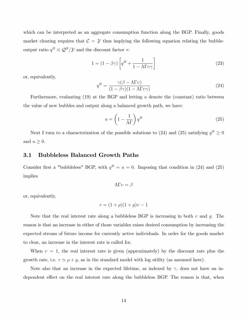
which can be interpreted as an aggregate consumption function along the BGP. Finally, goods

market clearing requires that C = Y thus implying the following equation relating the bubble-

output ratio qB � QB=Y and the discount factor �:

1 = (1� � )

�qB +

1

1� ���

�(23)

or, equivalently,

qB = (� � ���)

(1� � )(1� ��� ) (24)

Furthermore, evaluating (19) at the BGP and letting u denote the (constant) ratio between

the value of new bubbles and output along a balanced growth path, we have:

u =

�1� 1

��

�qB (25)

Next I turn to a characterization of the possible solutions to (24) and (25) satisfying qB � 0

and u � 0.

3.1 Bubbleless Balanced Growth Paths

Consider �rst a "bubbleless" BGP, with qB = u = 0. Imposing that condition in (24) and (25)

implies

��� = �

or, equivalently,

r = (1 + �)(1 + g)� � 1

Note that the real interest rate along a bubbleless BGP is increasing in both � and g. The

reason is that an increase in either of those variables raises desired consumption by increasing the

expected stream of future income for currently active individuals. In order for the goods market

to clear, an increase in the interest rate is called for.

When � = 1, the real interest rate is given (approximately) by the discount rate plus the

growth rate, i.e. r ' �+ g, as in the standard model with log utility (as assumed here).

Note also that an increase in the expected lifetime, as indexed by , does not have an in-

dependent e¤ect on the real interest rate along the bubbleless BGP. The reason is that, when

14

��� = �, such a change increases in the same proportion the present value of consumption and

that of income for any given real rate, making an adjustment in the latter unnecessary.21

Finally, note for future reference that in the bubbleless BGP considered here the real interest

rate r is lower than the growth rate g (i.e. �� > 1) if and only if � < �.

3.2 Bubbly Balanced Growth Paths

A BGP with a positive bubble corresponds to a solution to (24) and (25) satisfying qB > 0 and

u � 0. Thus, the existence of a BGP with a positive bubble, qB > 0, requires that

��� < �

On the other hand the non-negativity constraint on newly created bubbles u � 0 requires:

�� � 1

The two previous conditions are satis�ed if and only if

� < � (26)

If (26) is satis�ed, there exists continuum of bubbly BGPs fqB; ug indexed by r 2 (��=� �

1;��1]. Note that the condition for the existence of bubbly BGPs corresponds to the real interest

rate being less than the growth rate in the bubbleless BGP.

It can be easily checked that qB is increasing in r, with limr!g qB = (���)

(1�� )(1�� ) � qBmax, which

establishes an upper bound to the size of the bubble-output ratio, given �, and �. Note also that

@qBmax=@� < 0, i.e. the upper bound on the size of the bubble is decreasing in � over the range

� 2 [0; �], and converges to zero as � ! �.

One particular such bubbly BGP has no new bubbles introduced by new cohorts, i.e. u = 0.

Note that in that case

�� = 1

or, equivalently,

r = g

21The independence of the steady state real interest rate from is a consequence of the log utility speci�cationassumed here. That property is not critical from the viewpoint of the present paper, since there are other factors(the probability of retirement, in particular), that can drive real interest rate to values consistent with the presenceof bubbles.

15

with the implied bubble size given by qB = qBmax. Along that BGP any existing bubble will be

growing at the same rate as the economy. By contrast, along a bubbly BGP with bubble creation,

r < g implies that the size of the aggregate pre-existing bubble will be shrinking over time relative

to the size of the economy, with newly created bubbles �lling up the gap so that the size of the

aggregate bubble relative to the size of the economy remains unchanged.

Summing up, one can distinguish two regions of the parameter space relevant for the possible

existence of bubbly BGPs:

(i) � � � � 1. In this case, the BGP is unique and bubbleless and associated with a real

interest rate given by r = ��=� � 1 > g.

(ii) 0 < � < �. In this case multiple BGPs coexist. One of them is bubbleless, with r = r0 �

��=�� 1 < g. In addition, there exists a continuum of bubbly BGPs, indexed by the real interest

rate r 2 (r0; g], and associated with a bubble size (relative to output) qB 2 (0; qBmax], given by (24).

Figure 1 summarizes graphically the two regions with their associated BGPs.

3.3 A Brief Detour: Bubbly Equilibria and Transversality Conditions

Equilibria with bubbles on assets in positive net supply can be ruled out in an economy with an

in�nite lived representative consumer.22 In that economy, any positive net supply of that asset

must be necessarily held by the representative consumer, implying

limT!1

Et f�t;t+TAt+Tg � limT!1

Et��t;t+TQ

Bt+T (j)

Given that the bubble component of any asset must satisfy

limT!1

Et��t;t+TQ

Bt+T (j)

= QBt (j)

it follows that limT!1Et f�t;t+TAt+Tg � QBt (j). But the consumer�s transversality condition

requires that limT!1Et f�t;t+TAt+Tg = 0. Given that free disposal requires that QBt (j) � 0, it

follows that QBt (j) = 0 for all t.

Note that the previous reasoning cannot be applied to an overlapping generations economy

like the one developed above. The reason is that in that case it is no longer true that the positive

22See, e.g. Santos and Woodford (1997) for a discussion of the conditions under which rational bubbles can beruled out in equilibrium.

16

net supply of any bubbly asset must be held (asymptotically) by any individual agent, since it can

always be passed on to future cohorts (and it will in equilibrium). In fact, it is easy to check that

in the model above the individual transversality condition is satis�ed along any BGP, bubbly or

bubbleless. As shown in the appendix, for an individual born in period s � t it must be the case

that along any BGP

limT!1

TEt��t;t+TAt+T js

= 0

implying that the transversality condition is satis�ed along any admissible BGP. It is straightfor-

ward to show that this will be the case along any equilibrium that remains in a neighborhood of

a BGP, of the kind analyzed below.

3.4 Plausibility of Bubbly BGPs: Some Rough Numbers

Next I discuss plausible settings for the parameters of the model involved in the above characteri-

zation of the BGPs. To calibrate I use the expected lifetime at age 16, which is 63:2 years in the

U.S., and set = 1� 14�(62:3) ' 0:996. I use the average employment ratio (relative to population

aged 16 and over), which is (roughly) 0:6 on average over the period 1960-2016 as a proxy for �.

Conditional on the previous settings for � and one can derive � ' 0:9973. Thus, the analysis

above implies that the existence of bubbly balanced growth paths requires that � > 0:9973.

Unfortunately, the latter condition cannot be veri�ed easily since that parameter is not iden-

ti�ed by the above model once the existence of bubbles is allowed for. This is in contrast with the

standard representative agent model, for which there is a tight connection between the discount

rate and the real interest rate along a BGP.23 On the other hand, casual introspection suggests

that a discount factor of about 0:9 applied to utility 10 years from today (as implied by the lower

bound � = 0:9973) falls within the range of plausibility.

Alternatively, one may examine directly the relation between the average real interest rate,

r, and the average growth rate of output, g, two observable variables. As discussed above, the

existence of bubbly BGPs requires that r � g. Using data on 3-month Treasury bills, GDP de�ator

and (per capita) GDP, the average values for those variables in the U.S. over the period 1960Q1-

23Note that � = 0:9983 implies a discount factorof 0:9342 applied to utility 10 years from today, which seems entirely plausible.

17

2015Q4 are r = 1:4% � 4 = 0:35% and g = 1:6% � 4 = 0:4% (or, equivalently, � = 0:9965 and

� = 1:004), values which satisfy the inequality condition necessary for the existence of bubbles.

Note also that the above calibration implies ��� ' 0:9939, thus satisfying the condition for a

well de�ned intertemporal budget constraint.

For some of the quantitative analyses below I set the discount factor to be � = 0:998. This

is admittedly, an arbitrary choice, but it consistent with the existence of bubbly BGPs, with

associated real interest rates given by the interval [0:003348; 0:004].

4 Bubbles and Equilibrium Fluctuations

Having characterized the BGPs of the model economy, in the present section I shift the focus

to the analysis of the equilibrium dynamics in a neighborhood of a given BGP. In particular, I

am interested in determining the conditions under which equilibrium �uctuations unrelated to

fundamental shocks may emerge, as well as the role that variations in the size of the aggregate

bubble and the nature of monetary policy may play in such �uctuations.

As in the standard analysis of the NK model with a representative agent, I restrict myself to

equilibria that remain in a neighborhood of a BGP, and approximate the equilibrium dynamics by

means of the log-linearized equilibrium conditions.24 I leave the analysis of the global equilibrium

dynamics �including the possibility of switches between BGPs, the existence of a zero lower bound

on interest rates, and other nonlinearities�to future research. Secondly, in analyzing the model�s

equilibrium I ignore the existence of fundamental shocks, and focus instead on the possibility of

�uctuations driven by self-ful�lling expectations and on the role of bubbles as a source of those

�uctuations.25

I start by deriving the log-linearized equilibrium conditions around a BGP. In contrast with the

NK model with a representative agent, the individual consumer�s Euler equation and the goods

market clearing condition are no longer su¢ cient to derive an equilibrium relation determining

aggregate output as a function of interest rates (i.e. the so-called dynamic IS equation).26 In-

24See, e.g., Woodford (2003) or Galí (2015).25As the analysis of the equilibrium dynamics below will make clear, in the absence of bubbles and/or multiplicity

of equilibria the economy�s behavior in response to fundamental shocks involves no signi�cant di¤erences relativeto that of the standard New Keynesian model with a representative agent.26Formally, one can use the de�nition of aggregate consumption and the individual Euler equations to derive the

18

stead, the derivation of such a relation requires solving for an aggregate consumption function,

by aggregating the individual consumption functions obtained by combining the consumer�s Euler

equation and the intertemporal budget constraint. Since no exact representation exists for the

individual consumption function, I derive a log-linear approximation of that function around a

perfect foresight BGP. Then I aggregate the resulting individual consumption functions to obtain

an (approximate) aggregate consumption function. See the Appendix for detailed derivations.

The resulting representation of the equilibrium dynamics takes a very simple form, involving

only a few easily interpretable equations, as shown next.

Letting bct � log(Ct=�tC) and byt � log(Yt=�tY) denote log deviation of aggregate consumptionand output from their value along a BGP, the goods market clearing condition can be written as:

byt = bct (27)

As shown in the Appendix, the aggregate consumption function can be written, up to a �rst

order approximation, as follows: bct = (1� � )(bqBt + bxt) (28)

where bqBt � qBt � qB with qBt � QBt =(�tY) denoting the size of the aggregate bubble normalized

by trend output and where

bxt � 1Xk=0

(��� )kEtfbyt+kg � ���

1� ���

1Xk=0

(��� )kEtfbrt+kg (29)

is the fundamental component of aggregate wealth, i.e. the expected discounted sum of current and

future income), with brt =bit�Etf�t+1g denoting the real interest rate, andbit � log[(1+ it)=(1+r)]the nominal rate, all expressed in deviations from their values in the zero in�ation BGP.

Note that bxt can be conveniently rewritten in recursive form as:

bxt = ��� Etfbxt+1g+ byt � ���

1� ��� (bit � Etf�t+1g) (30)

Log-linearization of (19) around a BGP yields the equations describing �uctuations in the

aggregate bubble: bqBt = ��Etfbbt+1g � qB(bit � Etf�t+1g) (31)

aggregate relation:

Etfbct+1g = �bct +bit � Etf�t+1g�+ (1� )Etfbct+1jt+1gwhere Etfbct+1jt+1g cannot be expressed immediately as a function of bct:

19

bqBt = bbt + but (32)

where but � ut�u, with ut � Ut=(�tY) denoting the size of the newly introduced bubble normalized

by trend output and u its value along the BGP.

The New Keynesian Phillips curve derived above and given by

�t = ��� Etf�t+1g+ �byt (33)

completes the non-policy block of the system of di¤erence equations describing the model�s equi-

librium in a neighborhood of a BGP, where the latter is de�ned by a pair (qB;�) satisfying the

BGP conditions derived in the previous section.

In order to close the model a description of monetary policy is needed. To keep things as

simple as possible, in much of the analysis below I assume an interest rate rule of the form

bit = ���t + �qbqBt (34)

Note that the previous rule combines the usual �exible in�ation targeting motive (measured

by coe¢ cient ��, and consistent with a zero in�ation target) with a "leaning against the bubble"

one (parameterized by �q).27 In what follows, I assume the central bank takes as given the BGP

around which the economy �uctuates (and, hence, r and qB).

Equations (27) through (34) describe the equilibrium dynamics of the model economy in a

neighborhood of a given BGP. A quick glance at those equations makes clear that an outcome

with byt, �t, bqBt , but and the remaining variables all equal to zero at all times always constitutesa solution to the system of di¤erence equations. Thus, the perfect foresight BGP itself is always

an equilibrium. This should not be surprising, given that no fundamental shocks have been

introduced. The question of interest, however, is whether that outcome is the only possible

equilibrium and, more precisely, whether other equilibria exist involving aggregate �uctuations

that are bubble-driven. In order to isolate bubble-driven �uctuations, however, I also need to rule

out equilibria involving expectations-driven (i.e. sunspot) �uctuations unrelated to the existence

of bubbles. While the conditions that allow one to rule out such �uctuations in the standard

NK model are well known, it is important to check whether the introduction of �nite-lives and

retirement has, by itself, any consequences in that regard.27Given the close link between in�ation and the output gap implied by (33), there is little loss of generality (and

some gains in algebraic and expository convenience) in abstracting from a term involving the output gap in therule, as proposed in Taylor (1993).

20

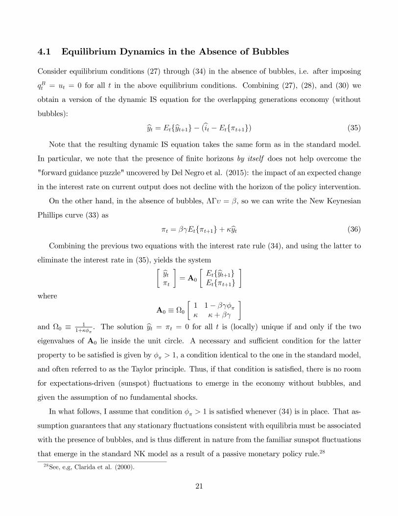
4.1 Equilibrium Dynamics in the Absence of Bubbles

Consider equilibrium conditions (27) through (34) in the absence of bubbles, i.e. after imposing

qBt = ut = 0 for all t in the above equilibrium conditions. Combining (27), (28), and (30) we

obtain a version of the dynamic IS equation for the overlapping generations economy (without

bubbles): byt = Etfbyt+1g � (bit � Etf�t+1g) (35)

Note that the resulting dynamic IS equation takes the same form as in the standard model.

In particular, we note that the presence of �nite horizons by itself does not help overcome the

"forward guidance puzzle" uncovered by Del Negro et al. (2015): the impact of an expected change

in the interest rate on current output does not decline with the horizon of the policy intervention.

On the other hand, in the absence of bubbles, ��� = �, so we can write the New Keynesian

Phillips curve (33) as

�t = � Etf�t+1g+ �byt (36)

Combining the previous two equations with the interest rate rule (34), and using the latter to

eliminate the interest rate in (35), yields the system� byt�t

�= A0

�Etfbyt+1gEtf�t+1g

�where

A0 � 0�1 1� � ��� �+ �

�and 0 � 1

1+���. The solution byt = �t = 0 for all t is (locally) unique if and only if the two

eigenvalues of A0 lie inside the unit circle. A necessary and su¢ cient condition for the latter

property to be satis�ed is given by �� > 1, a condition identical to the one in the standard model,

and often referred to as the Taylor principle. Thus, if that condition is satis�ed, there is no room

for expectations-driven (sunspot) �uctuations to emerge in the economy without bubbles, and

given the assumption of no fundamental shocks.

In what follows, I assume that condition �� > 1 is satis�ed whenever (34) is in place. That as-

sumption guarantees that any stationary �uctuations consistent with equilibria must be associated

with the presence of bubbles, and is thus di¤erent in nature from the familiar sunspot �uctuations

that emerge in the standard NK model as a result of a passive monetary policy rule.28

28See, e,g, Clarida et al. (2000).

21

4.2 Bubble-Driven Fluctuations

Nest I analyze the possibility of bubble-driven �uctuations in the OLG-NK model. Combining

equations (27), (28), and (30) one can obtain the dynamic IS equation:

byt = �Etfbyt+1g ���(bit � Etf�t+1g) +1� �

� (bqBt � ��� EtfbqBt+1g) (37)

where � � ����2 (0; 1] and � � 1��

1���� 2 (0; 1]. The previous equation can be combined with

(31) and (32) to yield byt = �Etfbyt+1g �(bit � Etf�t+1g) + �bqBt (38)

where � � (1�� )(1�� )�

> 0 and � ���1 + � (1��)

�(1�� )

�. Note that (38) has a form similar

to the dynamic IS equation in a standard NK model augmented with preference shocks, with

�uctuations in the bubble now playing the role of a demand shifter. In contrast with the standard

model though, the coe¢ cients on expected in�ation and interest rate will generally be di¤erent

from unity. In particular, the fact that ��� < � in a bubbly BGP implies that 0 < � < 1.

Accordingly, the impact on output of a given anticipated change in the interest rate declines with

the horizon, thus avoiding the extreme version of the so-called "forward guidance puzzle."29

In addition to (38), the equilibrium dynamics around a bubbly BGP are described by the bubble

equation (31), the New Keynesian Phillips curve (33), and the interest rate rule (34). Thus the

description of the equilibrium dynamics can be reduced to a four equation system, including three

equations that have the same interpretation as in the standard NK model, as well as a fourth

equation describing the evolution of the aggregate bubble.

Using (34) to eliminate the nominal interest rate in the remaining equilibrium conditions, we

can represent the resulting system of di¤erence equations in a compact way as follows:

A0xt = A1Etfxt+1g29The previous result can be shown to be linked to the fact that the factor ��� at which future income is

discounted when determining fundamental wealth (see (30)) di¤ers from the term � in the marginal propensityto consume in the presence of the bubble in the BGP, as implied by (23). This will also be the case in the presenceof an asset other than the bubble which is in (i) positive net supply, (ii) it is not a claim to future output, and (iii)which has a positive value for current consumers (net of liabilities associated with it, e.g. taxes). An example ofsuch an asset is government debt in the presence of �nite horizons, i.e. when Ricardian equivalence does not hold.The presence of such debt is key in accounting for the muting of the "forward guidance puzzle" in Del Negro et al.(2015).

22

where xt � [byt; �t; bqBt ]0 andA0 �

24 1 �� �q ���� 1 00 qB�� 1 + qB�q

35 ; A1 =

24 � 00 ��� 00 qB ��

35The solution to the previous dynamical system is (locally) unique if and only if the three

eigenvalues of the companion matrix A � A�10 A1 lie inside the unit circle. If that condition

is satis�ed, the equilibrium is given by byt = �t = bqBt = 0 for all t and, hence, it involves no

bubble-driven �uctuations. That uniqueness condition, however, is far from being guaranteed in

all cases, even for empirically plausible values of the rule coe¢ cients. This is illustrated in Figure 2,

which displays the uniqueness and indeterminacy regions on the (��; �q) plane, under alternative

assumptions regarding the real interest rate (and, hence, the bubble size) in the underlying BGP.

In addition to the baseline values for �, , and � introduced above, I assume � = 0:0424 as a

baseline value for the slope of the New Keynesian Phillips curve. That value is consistent with

� = 0:75 and ' = 0:5. The former setting is consistent with an average duration of individual

prices of 4 quarters, in accordance with much of the micro evidence. The setting for ' is consistent

with (12) and the observation that the standard deviation of the (log) real wage is roughly half

the size that of (log) hours worked (both HP-detrended), based on postwar U.S. data.

As shown in Figure 2, for r = 0:00335 �a value near the lower bound r0 consistent with a BGP�

indeterminacy is pervasive, independently of the value of �� and �q, at least for the range of those

coe¢ cients displayed in the Figure. It can be shown that, as r ! r0 this is the case for any value

of �� and �q Furthermore, if �� < 1, that indeterminacy is two-dimensional with the possibility of

expectations-driven bubble �uctuations added to the familiar source of indeterminacy associated

with a passive monetary policy. As one considers BGPs associated with larger bubble-output ratios

and higher real interest rates, we see that a region with a unique equilibrium emerges, and grows

larger as r increases. When the interest rate is close enough to its upper bound (r = g = 0:004),

the equilibrium is seen to be determinate whenever �� > 1, and even for a range of values of ��

less than one, as long as �q is positive.

For the sake of illustration, Figure 3 displays the simulated bubble-driven �uctuations, corre-

sponding to a calibration of the OLG-NK model consistent with one-dimensional indeterminacy.

In particular I assume r = 0:0035 (the estimated average interest rate in postwar U.S.), �� = 1:5

(the value proposed in Taylor (1993) and often used in related exercises) and �q = 0 (a likely

23

relevant value for the Fed and other central banks, at least before the �nancial crisis). Note that

in both the standard NK model and in the OLG-NK model without bubbles, the fact that �� > 1

would guarantee a unique equilibrium. By contrast, once bubbles are allowed for, that rule is

seen to be consistent with highly persistent �uctuations in output, in�ation and the bubble. The

intuition behind those �uctuations should be clear given the equilibrium relations discussed above:

if, starting from a BGP, individuals become "optimistic" and expect bubble assets to command

a higher price in the future they will be willing to pay a higher price for those assets today; the

resulting increase in �nancial wealth will raise aggregate demand, which �rms will be willing to

meet by increasing output. The consequent reduction in average markups will lead �rms which

can adjust their prices to raise them, thus generating positive in�ation. The endogenous pol-

icy response to the higher in�ation partly dampens the increase in aggregate demand, but not

su¢ ciently to fully stabilize it.

How e¤ective is a monetary policy that leans against the bubble, as captured by a positive value

for �q, at preventing the possibility of bubble-driven �uctuations? Figure 4 seeks to answer that

question by showing the threshold value for �q above which stationary bubble-driven �uctuations

can be ruled out, given �� = 1:5. As the �gure makes clear, the extent to which a systematic

interest rate response to the aggregate bubble may rule out such �uctuations depends very much

on the steady state real interest rate (and, hence on the size of the bubble-output ratio along

the corresponding BGP). As discussed above, if the interest rate is close enough to the growth

rate (i.e. bubble-output ratio is su¢ ciently large), a policy that focuses on stabilizing in�ation is

su¢ cient to prevent bubble-driven �uctuations, even with �q = 0. To see why this is the case it is

useful to combine (31) and (32) to yield:

bqBt = (��)�1bqBt�1 + qBbrt�1 + "t

where "t � bt � Et�1fbtg+ ut denotes the aggregate bubble innovation. When the bubble-output

ratio qB is large and the interest rate is close to the growth rate (�� . 1) a policy that involveseven a small response of the real rate to a larger bubble will trigger an explosive path for the

latter, inconsistent with an equilibrium. On the other hand, as qB approaches zero and (��)�1

diverges from unity, it takes an ever more aggressive interest rate response in order to rule out the

possibility of stationary �uctuations in the aggregate bubble (and, hence, in output and in�ation).

24

This is captured in Figure 4 which shows how the threshold value for �q rises quickly as r declines,

and becomes in�nite as that variable approaches 0:0033, its lower bound.

4.2.1 A Particular Case: Bubble-Driven Fluctuations around the Bubbleless BGP

The previous analysis has focused on �uctuations in a neighborhood of a perfect foresight bubbly

BGP. But given the existence of a continuum of such BGPs one may wonder why an economy

would tend to gravitate towards the same one. From that viewpoint, the possibility of bubble-

driven �uctuations near a bubbleless BGP may be viewed as particularly appealing since that BGP

would seem to be a natural "attractor" in the face of a bursting aggregate bubble. The present

section focuses on that particular case.

Note that in a neighborhood of the bubbleless BGP the aggregate bubble qBt must now satisfy

the equilibrium conditions

qBt = (�=�)Etfbt+1g (39)

qBt = bt + ut (40)

where (qBt ; ut) � 0 for all t. Note that the assumption qB = 0 made here implies that interest rate

changes do not a¤ect (up to a �rst order approximation) the expected evolution of the bubble,

which simpli�es the analysis considerably. Furthermore, under the maintained assumptions that

� < � (implying r < g) and 0 < ut < u for all t, it is easy to check that limk!1EtfqBt+kg < u1��=� ,

i.e. the bubble is non-explosive and its average long run value can be made arbitrarily close to

zero.

The previous environment allows for the possibility of recurrent booms and busts driven by

an exogenous stochastic bubble of the kind proposed in Blanchard (1979). To illustrate that

possibility, consider a bubble that evolves according to the process.

qBt =

����qBt�1 + ut with probability �

ut with probability 1� �(41)

where futg follows a martingale-di¤erence process with positive support and constant mean u & 0.It is easy to check that the previous process satis�es (39) and (40), as well as the non-negativity

condition. Note that the aggregate bubble will display persistent �uctuations over time, experienc-

ing recurrent (though unpredictable) collapses, before being rekindled again by newly introduced

bubbles.

25

The previous stochastic bubble process can be combined with (33), (34), and (37), all evaluated

at the perfect foresight bubbleless BGP (i.e. with ��� = � and qB = 0) to describe the equilibrium

dynamics. In the special case considered here, the equilibrium output gap and in�ation can be

solved for in closed form, as a function of the current value of the aggregate bubble:

byt = (1� � )(�� �q)qBt

�t = �(�� �q)qBt

where � 1=[(1� � )(1� �=�) + �(�� � �=�)] > 0.

Figure 5 displays a simulated equilibrium path generated by the previous model. In addition

to the baseline parameter settings introduced above, I set � = 0:95 as a value describing the

process for the bubble and draw futg from a uniform distribution on [0; 0:001]. As above I assume

�� = 1:5 and �q = 0. Note that the simulated �uctuations display a characteristic "boom-bust"

pattern often found in accounts of historical bubble episodes, with the output gap and in�ation

moving in step with the bubble.

5 Bubbles and Monetary Policy Design

In the present section I discuss the implications of alternative monetary policies in the OLG-NK

economy developed above. For concreteness, I adopt the perspective of a central bank that seeks

to stabilize in�ation.30 Note that the lack of a trade-o¤ between in�ation and output gap implied

by (33) makes an in�ation targeting policy also consistent with output gap stabilization. Next I

discuss three candidate strategies to implement that in�ation targeting policy.

A �rst strategy, implicit in the analysis above, consists in adopting a rule that would render

bubble-driven �uctuations inconsistent with equilibrium. As discussed in section 4, a su¢ ciently

aggressive "leaning against the bubble" policy, implemented by means of an interest rate rule like

(34) with a large setting for �q may in some instances serve that purpose. An important limitation

of such a strategy is that if the economy is too close to the bubbleless BGP, there may not be a

�nite value of �q that would make that strategy feasible, or the required value for �q may be far

too large, which would render it unfeasible in practice.

30The presence of uninsurable cohort-speci�c shocks linked to new bubbles renders the analysis of the fullyoptimal monetary policy hard to tackle. I leave its exploration for future research.

26

Rather than ruling out equilibria involving bubble �uctuations, an alternative policy strategy

would instead seek to o¤set the e¤ects of those �uctuations on aggregate demand, through a

suitable adjustment in the interest rate. Given (38), that policy can be implemented with the rule

bit = ���t + (�=)bqBt (42)

where �� > 1. Combining (42) with (38) and (33), one can check that the equilibrium is locally

unique and given by byt = �t = 0 for all t. In other words, that policy would succeed in fully

insulating aggregate output and in�ation from �uctuations in the bubble. Note, however, that

such a policy would not prevent �uctuations in the bubble. Instead, the latter would evolve in

equilibrium according to: bqBt = �bqBt�1 + "t (43)

where "t � bt�Et�1fbtg+but and � � 1��

�1 + qB�

�, with the latter being less than one under the

conditions that allow for non-explosive bubble-driven equilibria, as discussed above. Note that this

in turn requires that qB is su¢ ciently small.31 As long as that condition is satis�ed, the aggregate

bubble will display non-explosive �uctuations around its BGP value, as described by (43), but

those �uctuations will not translate into output or in�ation �uctuations, for the response of the

nominal (and real) interest rate will exactly o¤set their impact on aggregate demand.

The same outcome, however, could be approximated if the central bank were to adopt a rule

that directly targeted in�ation and/or the output gap, while ignoring the existence of a bubble

and its eventual �uctuations. If that rule were indeed to succeed in stabilizing in�ation, then it

would have to be the case that, in equilibrium, bit = (�=)bqBt , as implied by (38). An example ofsuch a rule is given by bit = ���t with �� arbitrarily large. The main advantage of such a strategy,

relative to the �rst one is that it is always e¤ective, even in the limiting case when �uctuations

emerge near the bubbleless BGP. Relative to the second strategy, a direct in�ation targeting rule

does not require that the bubble be observed nor knowledge of the model�s parameters.

Figure 6 illustrates the previous point by displaying the standard deviation of the output

gap as a function of �� and �q, given r = 0:0035, and keeping the remaining parameter settings

unchanged. The �gure points to the potential destabilizing e¤ects of a "leaning against the bubble"

31Note that limqB!0 � = �=� which is less than one under the conditions that guarantee the existence of bubbles.

27

policy that is not "surgically" calibrated, and which stands in contrast to the greater robustness

of in�ation targeting policies, which can approximate the desired outcome arbitrarily well.

Figure 7 displays the standard deviation of the bubble, as a function of �� and �q, and under

an identical calibration of the remaining parameters. The �gure illustrates a somewhat surprising

aspect of "leaning against the bubble" policies: contrary to conventional wisdom, such policies

may end up increasing the size of bubble �uctuations. That outcome, already uncovered in Galí

(2014) in the context of a two-period monetary OLG model, follows from the requirement that

any existing bubble grows (in expectation) at the rate of interest. Thus, if the latter increases

with the bubble, the size of bubble �uctuations may be ampli�ed. To the extent that those

�uctuations are deemed undesirable �beyond their e¤ects on the output gap and in�ation�the

previous �nding provides an additional argument against policies that directly (and aggressively)

respond to �uctuations in the bubble.

6 Concluding Comments

The NK model remains the workhorse framework for monetary policy analysis, even though it

is unsuitable �in its standard formulation�to accommodate the existence of asset price bubbles

and hence to address one of the key questions facing policy makers, namely, how monetary policy

should respond to those bubbles. That shortcoming, however, is not tied to any key ingredient of

the model (e.g. staggered price setting), but to the convenient (albeit unrealistic) assumption of

an in�nite-lived representative consumer. In the present paper I have developed an extension of

the basic NK model featuring overlapping generations, �nite lives and (stochastic) transitions to

inactivity. In contrast with the standard model, the OLG-NK framework allows for the existence

of rational expectations equilibria with asset price bubbles. In particular, plausible calibrations

of the model�s parameters are consistent with the existence of a continuum of bubbly balanced

growth paths, as well as a bubbleless one (which always exists). When combined with sticky prices,

�uctuations in the size of the aggregate bubble, possibly unrelated to changes in fundamentals,

are a potential source of �uctuations in output and in�ation.

The analysis of the properties of the model has yielded several insights regarding its implications

for monetary policy.

Firstly, when one abstracts from the possibility of bubbly equilibria, the introduction of an

28

overlapping generations structure does not change any of the qualitative properties of the standard

NK model. In particular, the Taylor principle still de�nes the condition under which a simple

interest rate rule guarantees equilibrium uniqueness. Furthermore, the presence of �nite horizons

by itself does not help overcome the so called "forward guidance puzzle" uncovered by a number

of authors in the context of an in�nitely-lived representative agent model.

Secondly, a "leaning against the bubble" interest rate policy, if precisely calibrated, may succeed

in insulating output and in�ation from aggregate bubble �uctuations. However, mismeasurement

of the bubble or an inaccurate "calibration" of the policy response to bubble �uctuations may end

up destabilizing output and in�ation. On the other hand, and contrary to conventional wisdom,

a "leaning against the bubble" policy, even when precisely implemented, does not guarantee the

elimination of the bubble or the dampening of its �uctuations. In fact, under some conditions

such a policy may end up increasing the volatility and persistence of bubble �uctuations. By way

of contrast, a policy that targets in�ation directly may attain the same stabilization objectives

without the risks associated with a "direct" response to the bubble.

Four additional remarks, pointing to possible future research avenues are in order. Firstly,

the analysis of the equilibrium dynamics above has assumed "rationality" of asset price bubbles.

That assumption underlies the equilibrium conditions that individual and aggregate bubbles must

satisfy, i.e. (17) and (19), respectively, and the implied log-linear approximation (31). However,

the remaining equilibrium conditions, including the modi�ed dynamic IS equations, are still valid

even if the process followed by the aggregate bubble were to deviate from that of a rational bubble.

That observation opens the door to analyses of the macroeconomic e¤ects and policy implications

of alternative speci�cations of the aggregate assets misvaluations.

Secondly, the analysis above suggests that, in the absence of other frictions, the rise and fall of

an aggregate bubble is likely to have small quantitative e¤ects on aggregate demand and, hence,

on output and in�ation. To the extent that the historical evidence points to a larger macro impact

of bubbles, there may be additional channels through which that impact operates. The work of

Farhi and Tirole (2011), Martin and Ventura (2012), and Asriyan et al. (2016), emphasizing the

interaction of the bubble with �nancial frictions, points to a possible source of larger quantitative

e¤ects that one might be able to incorporate in the above framework.

Thirdly, balanced growth paths characterized by a larger bubble size are associated with a

29

higher real interest rate. Thus, the presence of a bubble along a BGP should make it less likely

for the zero lower bound on the nominal interest rate to become binding, ceteris paribus and

conditional on the bubble not bursting. Similarly, the bursting of the bubble would bring along

a reduction in the natural rate of interest that could pull the interest rate toward the zero lower

bound. The analysis of the interaction of bubble dynamics with the zero lower bound seems an

avenue worth exploring in future research.

Finally, the analyses of the equilibrium dynamics above has assumed that the central bank

takes as given the BGP on which the economy settles and, hence, its associated real interest rate.

That assumption is re�ected in the implicit exogeneity of the real interest rate term embedded

in the policy rule through the term bit ' it � r. But while that assumption is a natural one in

the context of economies whose real interest rate along a BGP is uniquely pinned down (as it is

the case in the standard New Keynesian model with a representative consumer), it is no longer

so in an economy like the one analyzed above, in which a multiplicity of real interest rates may

be consistent with a perfect foresight BGP. Future research should explore the implications of

relaxing the assumption of a policy invariant steady state real interest rate.

30

References

Allen, Franklin, Gadi Barlevy and Douglas Gale (2017): "On Interest Rate Policy and Asset

Bubbles," mimeo.

Asriyan, Vladimir, Luca Fornaro, Alberto Martín and Jaume Ventura (2016): "Monetary

Policy for a Bubbly World," mimeo.

Bernanke, Ben S. (2002): "Asset Price Bubbles and Monetary Policy," speech before the New

York Chapter of the National Association of Business Economists.

Bernanke, Ben S. and Mark Gertler (1999): "Monetary Policy and Asset Price Volatility," in

New Challenges for Monetary Policy, Federal Reserve Bank of Kansas City, 77-128.

Bernanke, Ben S. and Mark Gertler (2001): "Should Central Banks Respond to Movements in

Asset Prices?" American Economic Review 91(2), 253-257.

Blanchard, Olivier J. (1979): "Speculative Bubbles, Crashes and Rational Expectations," Eco-

nomic Letters 3, 387-389.

Blanchard, Olivier J. (1985): "Debt, De�cits, and Finite Horizons." Journal of Political Econ-

omy, 93(2), 223-247.

Borio, Claudio and Philip Lowe (2002): "Asset Prices, Financial and Monetary Stability:

Exploring the Nexus," BIS Working Papers no. 114.

Carvalho, Carlos, Andrea Ferrero and Fernanda Nechio (2016): "Demographics and real inter-

est rates: Inspecting the Mechanism," European Economic Review, forthcoming.

Cecchetti, Stephen G., Hans Gensberg, John Lipsky and Sushil Wadhwani (2000): Asset Prices

and Central Bank Policy, Geneva Reports on the World Economy 2, CEPR.

Del Negro, Marco, Marc Giannoni, and Christina Patterson (2015): "The Forward Guidance

Puzzle," unpublished manuscript.

Dong, Feng, Jianjun Miao, Pengfei Wang (2017): "Asset Bubbles and Monetary Policy,"

mimeo.

Farhi, Emmanuel and Jean Tirole (2011): "Bubbly Liquidity." Review of Economic Studies

79(2): 678-706.

Galí, Jordi (2014): "Monetary Policy and Rational Asset Price Bubbles," American Economic

Review, vol. 104(3), 721-752

Gertler, Mark (1999): "Government Debt and Social Security in a Life-Cycle Economy,"

31

Carnegie-Rochester Conference Series on Public Policy 50, 61-110.

Kohn, Donald L. (2006): "Monetary Policy and Asset Prices," speech at an ECB colloquium

on "Monetary Policy: A Journey from Theory to Practice," held in honor of Otmar Issing.

Kohn, Donald L. (2008): "Monetary Policy and Asset Prices Revisited," speech delivered at

the Caton Institute�s 26th Annual Monetary Policy Conference, Washington, D.C.

Martín, Alberto, and Jaume Ventura (2012): "Economic Growth with Bubbles," American

Economic Review, vol.102(6), 3033-3058.

McKay, Alisdair, Emi Nakamura, and Jón Steinsson (2016). "The Power of Forward Guidance

Revisited," American Economic Review 106 (10): 3133-3158.

Nisticò, Salvatore (2012): "Monetary Policy and Stock-Price Dynamics in a DSGE Frame-

work," Journal of Macroeconomics 34, 126-146.

Piergallini, Alessandro (2006): "Real Balance E¤ects and Monetary Policy," Economic Inquiry

44(3), 497-511.

Samuelson, Paul A. (1958): "An Exact Consumption-Loan Model of Interest with or without

the Social Contrivance of Money," Journal of Political Economy 66, 467-482.

Santos, Manuel S. and Michael Woodford (1997): "Rational Asset Pricing Bubbles," Econo-

metrica 65(1), 19-57.

Schularick, Moritz and Alan M. Taylor (2012): "Credit Booms Gone Bust: Monetary Policy,

Leverage Cycles and Financial Crises, 1870-2008" American Economic Review, 102(2), 1029-1061.

Taylor, John (2014): "The Role of Policy in the Great Recession and the Weak Recovery,"

American Economic Review 104(5), 61-66.

Tirole, Jean (1985): "Asset Bubbles and Overlapping Generations," Econometrica 53, 1499-

1528.

Yaari, Menahem E. (1965): "Uncertain Lifetime, Life Insurance, and the Theory of the Con-

sumer," The Review of Economic Studies, 32(2), 137-150

32

TECHNICAL APPENDIX

1. Transversality condition in a Bubbly BGP

The consumption function for an active individual born in period s is:

Cat+T js = (1� � )

�Aat+T js +

Wt+TN=�

1� ���

�In particular:

Catjs = (1� � )

�Aatjs +

WtN=�

1� ���

�In addition, Ct+T js = (�=�)TCtjs thus implying

Aat+T js = (�=�)T

�Aatjs + (1� (��=�)T )

WtN=�

1� ���

�On the other hand, for a retired individual

Crtjs = (1� � )Artjs

Using the fact that Crtjs = Catjs we have:

Artjs = Aatjs +WtN=�

1� ���

The transversality condition for an active individual takes the form:

limT!1

( �)TEtfAt+T jsg = limT!1

( �)T [�TAat+T js + (1� �T )Art+T js]

= limT!1

( �)T [Aat+T js + (1� �T )�TWtN=�

1� ��� ]

= limT!1

(� )T�Aatjs + (1� (��=�)T )

WtN=�

1� ���

�+ limT!1

( ��)T (1� �T )WtN=�

1� ���

=WtN=�

1� ��� limT!1

[(� )T � (�� )T + (�� )T � (��� )T ]

= 0

where the maintained assumption ��� < 1 has been used.

2. Log-linearized individual intertemporal budget constraint

33

The intertemporal budget constraint as of period t for an individual born in period s and still

active in period t � s can be derived by iterating (3) forward to yield:

1Xk=0

kEtf�t;t+kCt+kjsg = Aatjs +1

�

1Xk=0

( �)kEtf�t;t+kWt+kNt+kg (44)

For retired individuals, the corresponding constraint is:1Xk=0

kEtf�t;t+kCt+kjsg = Artjs (45)

Letting lowercase letters with a "^" symbol denote the log deviation of a variable from its value

along a perfect foresight balanced growth path (BGP), the left hand side term of (44) and (45)

can be approximated in a neighborhood of the BGP as:1Xk=0

kEtf�t;t+kCt+kjsg ' �tCt�s1� �

+ �t1Xk=0

(�� )kCt+k�sEtfbct+kjs + b�t;t+kg=

�tCt�s1� �

+�tCt�s1� �

bctjswhere Cj denotes consumption of an individual aged j, normalized by current productivity, along a

BGP, b�t;t+k = log(�t;t+k=�k), and where I have made use of the fact that Ct+k�s = [�(1+r)=�]kCt�sand Etfb�t;t+k + bct+kjsg = bctjs (resulting from (4)).

The second term on the right hand side of (44), which is relevant only for active individuals,

can be approximated around the BGP as:

1

�

1Xk=0

(� )kEtf�t;t+kWt+kNt+kg '�tWN

�(1� ��� ) +��tWN

�

� 1Xk=0

(��� )kEtf bwt+k + bnt+k + b�t;t+kgwhere W is the wage along the BGP, normalized by productivity.

3. Aggregation and derivation of log-linearized aggregate consumption Euler equa-

tion

Let C denote aggregate consumption (normalized by current productivity), along the BGP.

One can derive the approximate relations Cbct = (1� )Pt

s=�1 t�sCt�sbctjs and the BGP relation

C = (1� )Pt

s=�1 t�sCt�s. Those relations can be used to aggregate the log-linearized individual

consumption functions across all individuals to yield:

�tC1� �

+�tC1� �

bct = (QFt +QBt ) +�tWN

1� ��� + �tWN

1Xk=0

(��� )kEtf bwt+k + bnt+k + b�t;t+kg34

Note also that in a neighborhood of the BGP,

QFt =1Xk=0

(� )kEtf�t;t+kDt+kg

' �tD1� ��� + �

tD1Xk=0

(��� )kEtfbdt+k + b�t;t+kgwhere D denotes aggregate dividends (normalized by productivity), along a BGP.

Thus, using the approximation byt = (WN=Y)( bwt + bnt) + (D=Y)bdt, the BGP relation �tC1�� =

QB + �t(WN+D)1���� , and the goods market clearing condition Y = C, we obtain the log-linearized

aggregate consumption function

bct = (1� � )

"bqBt + 1Xk=0

(��� )kEtfbyt+k + b�t;t+kg#

= (1� � )

"bqBt + 1Xk=0

(��� )kEtfbyt+kg � 1Xk=1

(��� )kk�1Xj=0

Etfbrt+jg#

= (1� � )

"bqBt + 1Xk=0

(��� )kEtfbyt+kg � ���

1� ���

1Xk=0

(��� )kEtfbrt+kg#

where bqBt � qBt � qB, with qBt � QBt =(�tY) and qB its corresponding value along a BGP, andbrt �bit � Etf�t+1g.

Note that we can write the consumption function more compactly as:

bct = (1� � )(bqBt + bxt) (46)

where bxt �P1k=0(��� )

kEtfbyt+kg � ��� 1����

P1k=0(��� )

kEtfbrt+kg is the "fundamental" compo-nent of wealth, expressed in log deviations from its value along a BGP. It satis�es the recursive

equation: bxt = ��� Etfbxt+1g+ byt � ���

1� ��� brtFurthermore, log-linearization of (??) about a BGP yields:

bqBt = ��EtfbqBt+1g � qBbrt (47)

35

In a neighborhood of the bubbleless BGP qB = 0 and ��� = �, thus implying the approximate

aggregate Euler equation:

bct = � Etfbct+1g+ (1� � )(1� � )qBt + (1� � )byt � � brtImposing goods market clearing (bct = byt) and rearranging terms, we obtain a dynamic IS

equation: byt = Etfbyt+1g+ �qBt � brtwhere � � (1 � � )(1 � � )=� > 0 and fqBt g must satisfy qBt = (�=�)EtfqBt+1g and qBt � 0 for

all t.

Note that in a bubbleless equilibrium around the bubbleless BGP:

byt = Etfbyt+1g � brtwhich is identical to the standard dynamic IS equation of the representative consumer model.

In any bubbly steady state, qB = 11�� �

11���� . Combining (46) and (47) yields the Euler

equation: bct = ��� Etfbct+1g+ (1� � )(1� � )bqBt + (1� � )byt ��� brtwhere � �

�1 + (1�� )(���1)

1����

�> 1 and � 2

�1; �

��

�. Imposing goods market clearing:

byt = ���

�Etfbyt+1g+ �bqBt � ��� brt (48)

In the particular case of � = 0, we have �� = � = 1 thus implying a dynamic IS equation of

the form: byt = �

�Etfbyt+1g+ �bqBt � �

�brt

4. Conditions for equilibrium uniqueness around the bubbleless BGP.

The necessary and su¢ cient conditions for AT to have two eigenvalues within the unit circle

are: (i) j det(AT )j < 1 and (ii) jtr(AT )j < 1 + det(AT ) (LaSalle (1986)). Note that in the case

of a bubbleless BGP, det(AT ) =�

1+���> 0 while tr(A0) =

1+�+�1+���

> 0. Condition (i) requires

�� > (�� 1)=�. Condition (ii) corresponds to �� > 1.

36

5. Sunspot Fluctuations

Let the equilibrium be described by the system of di¤erence equations

xt = AEtfxt+1g

where xt � [byt; �t; bqBt ]0 are all non-predetermined variables. Let A have q � 3 eigenvalues with

modulus less than one.

Consider the transformation xt = Qvt where QJQ�1 = A where J is the canonical Jordan

matrix and Q � [q(1);q(2);q(3)] is the matrix of generalized eigenvectors, corresponding to the

three eigenvalues. Thus,

vt = JEtfvt+1g

where J =�Ju 00 Js

�and vt = [vut , v

st ]0.

Consider the case where A has two eigenvalues with modulus less than one and one with

modulus greater than one. For concreteness, assume j�1j < 1; j�2j < 1; and j�3j > 1. If all

eigenvalues are real Ju =��1 00 �2

�, Js = �3, and q(k) corresponds to the eigenvector associated

with eigenvalue k; for k = 1; 2; 3. Otherwise, if �1 = a+bi and �2 = a�bi are complex conjugates,

Ju =

�a �bb a

�; Js = �3 and q(1) and q(2) are, respectively, the imaginary and real components

of the eigenvector associated with the complex eigenvalues.

Thus, vut = 0 all t: In addition vst = �3Etfvst+1g; which has a stable solution:

vst = ��13 vst�1 + �t

where �t is a martingale-di¤erence (univariate) process.

Thus, we have xt = q(3)vst is the sunspot solution. The three variables in xt will be perfectly

correlated (positively or negatively), and will display a �rst-order autocorrelation ��13 . In the

simulations reported normalize the the third element of q(3) to unity, in which case the innovation

in vst (denoted by �t) corresonds to the innovatin in the bubble.

Consider next the case where A has one eigenvalue with modulus less than one and two with

modulus greater than one. For concreteness, assume j�1j < 1; j�2j > 1; and j�3j > 1. If all

eigenvalues are real Ju = �1, Js =��2 00 �3

�and q(k) corresponds to the eigenvector associated

with eigenvalue k; for k = 1; 2; 3. Otherwise, if �2 = a+bi and �3 = a�bi are complex conjugates,

Ju = �1, Js =�a �bb a

�and q(2) and q(3) are, respectively, the imaginary and real components

37

of the eigenvector associated with the complex eigenvalues, while q(1) is the eigenvector associated

with �1.

Thus, vut = 0 all t: In addition vst = JsEtfvst+1g; which has a stable solution:

vst = J�1s v

st�1 + �t

where �t is a (bivariate) martingale-di¤erence process.

Thus, we have xt = [q(2);q(3)]vst is the sunspot solution. We can normalize the third element

of q(2) and q(3) to unity.

38

Figure 1. Balanced Growth Paths

Figure 2. Determinacy and Indeterminacy Regions

Figure 3. Simulated Bubble-driven Fluctuations

around a Bubbly BGP

20 40 60 80 100 120 140 160 180 200

time

0

0.05

0.1

bubble size

20 40 60 80 100 120 140 160 180 200

time

0

5

10

15

10 -7 output

20 40 60 80 100 120 140 160 180 200

time

-2

0

2

4

6

8

10

10 -6 inflation

Figure 4. The Effectiveness of “Leaning against the Bubble” Policies

Figure 5. Simulated Bubble-Driven Fluctuations

around the Bubbleless BGP

0 50 100 150 200 250 300 350 400

bubble size

0

0.1

0.2

0.3

0 50 100 150 200 250 300 350 400

output

0

2

410 -4

0 50 100 150 200 250 300 350 400

inflation

0

0.005

0.01

Figure 6. Bubble-Driven Fluctuations:

Monetary Policy and Macro Volatility

0.5

3

1

1

1.5

2

10 -5

2.5

2.5 0.8

3

3.5

0.610 -4

2 0.41.5 0.2

0

Figure 7. Bubble-Driven Fluctuations:

Monetary Policy and Bubble Volatility

0.3864

3

0.38645

12.5 0.8

0.3865

0.6

0.38655

10 -420.4

1.5 0.20