monetary aspects of bahmani copper coinage in light of the …coinindia.com/akola.pdf ·...
TRANSCRIPT

Monetary Aspects of Bahmani Copper Coinage
in Light of the Akola Hoard
Phillip B. Wagoner and Pankaj Tandon
Draft: 9/24/16
**Please do not quote or disseminate without permission of the authors**

1
The Bahmanis of the Deccan produced copper coinage from the very outset of the state’s
founding in AH 748/1347 CE, but it was clearly secondary to the silver tankas upon which their
monetary system was based. By the first several decades of the fifteenth century, however, as John
Deyell has shown, the relative production values of silver and copper coinage had reversed, and there
was an enormous expansion in copper output, both in terms of the numbers of coins produced and in
terms of the range of their denominations (Fig.1).1 This phenomenon has attracted the attention of
several scholars, but fundamental questions yet remain about the copper coinage and how it functioned
within the Bahmani monetary system. Given the dearth of contemporary written documents shedding
light on these matters, it is understandable that many would simply give up on trying to answer these
questions. But to do so would be to ignore the physical, material evidence afforded in abundance by the
coinage itself, including such aspects as its metrology and denominational structure, and most
importantly, the indications of its usage patterns embodied within the composition and geographic
distribution of individual coin hoards. Ultimately, we may wish to know why Bahmani copper coinage
production should have undergone such a sudden expansion in the 1420s and 1430s, but in order to
realize this goal, we must first address the physical nature of the coinage itself and what it can tell us
about how it was used.
1 John Deyell, e-mail communication, 23 May, 2013.

2
Figure 1 (courtesy of John Deyell)
This essay represents an attempt to move in this direction through detailed analysis of an intact
hoard of 713 Bahmani copper coins from Akola in Maharashtra, now in the collection of the Indian
Institute for Research in Numismatic Studies (IIRNS) in Nasik.2 As the reader will see, the data
provided by this hoard sheds light on the denominational structure of the Bahmani copper coinage and
what that in turn implies about how these abundant copper coins were used, and my members of which
social groups. The hoard also provides a sample of sufficiently large size to permit measuring the rate of
weight loss through circulation, the variation in that rate from one denomination to another, and what
this implies about the different velocities at which the various denominations circulated. Finally, the
hoard has also afforded us the opportunity to develop a scientifically grounded method for determining
the target mint weight for a given denomination through regression estimates.
2 We gratefully acknowledge the hospitality and support afforded by Kamal K. Maheshwari, Amiteshwar Jha and the entire
staff of IIRNS during our stay there in early 2016. The second author was in India on a Fulbright-Nehru Fellowship; that
support is also gratefully acknowledged.

3
The limitations of a study restricted to a single hoard are of course considerable. For one thing,
the non-existence of statistical data on other Bahmani copper hoards greatly constrains the specific types
of analysis that we are able to offer here.3 Comparative study of the structure of numerous hoards, for
example—such as is possible with Roman coin hoards4—is simply not yet an option in the case of
Bahmani hoards. Accordingly, we have little choice but to begin with a detailed analysis of a single
intact hoard, and to hope that others will eventually come to light, making it possible to carry out more
varied kinds of analysis in the future. It is clear from the treasure trove reports published annually in
Indian Archaeology—a Review that substantial numbers of Bahmani hoards have been found and
reported, even if they have not yet been properly published or subjected to statistical analysis, so it is not
unreasonable to expect that other hoards will become available.5
Before going into the details of the Akola hoard, it may be useful to review briefly the salient
features of the Bahmani currency system.6 Bahmani coinage originated as an adaptation of that
employed by the Delhi Sultanate in north India, which, by the time it was introduced to the Deccan with
Delhi’s conquests of the region in about 1300, had already been refined through nearly a century’s use in
the subcontinent. The Bahmanis’ adaptation included two heavy gold denominations, the dinār and the
3 It would appear that no hoard of Bahmani coppers has previously been subjected to fine-grained statistical analysis such as
that presented here. Indeed, the only published hoard of Bahmani coppers of which we are aware is Khwaja Ghulamus
Syedain’s article on a smaller hoard (103 coins) from Ladkhed, also in Maharashtra. See Syedain, “Ladkhed Hoard of
Bahmani Copper Coins from Maharashtra,” Studies in South Indian Coins 7(1997): 95-104. Unfortunately, this does not
record the weights or dates of the individual coins, but only provides an average weight for each type.
4 See, for example, Kris Lockyear, “Multivariate Money: A Statistical analysis of Roman Republican coin hoards with
special reference to material from Romania,” University College London, doctoral thesis, 1996, and idem., Patterns and
Process in Late Roman Republican Hoards, 157 – 2 B.C., BAR International Series, vol. 1733, Oxford: 2007.
5On the utility of the Treasure Trove Reports, and for the details of a spatial database constructed by Wagoner in 2012-2013,
which plots the findspots and compositions of over 300 hoards from the Deccan containing coins issued by the Bahmanis or
by Vijayanagara, see Wagoner, “Money use in the Deccan, c. 1350-1687: The role of Vijayanagara hons in the Bahmani
currency system”, Indian Economic and Social History Review 51/4(Oct.-Dec. 2014): 457-480.
6 The information in this paragraph is largely based on Stan Goron and J.P. Goenka, The Coins of the Indian Sultanates (New
Delhi: Munshiram Manoharlal, 2001), pp.285-310.

4
tanka, weighing respectively 14 and 12 māṣas7 (12.85 and 11.02 g), and minted at close to 100 per cent
purity. Because of the amount of gold they contain, these were clearly high-value coins that would have
been useful only for the highest value monetary transactions, or else as a medium for storing wealth. For
other purposes, the silver tanka, weighing 12 māṣas (11.02 g) would have been used, together with four
fractional silver denominations from the two-thirds unit down to the one-twelfth. Initially, a copper
coin—minted at 4 māṣas (3.67 g)—and its half and quarter fractions would have served for everyday
transactions in the bazaar. This was soon augmented with a growing array of larger denominations, until
by the middle of the fifteenth century as many as nine different copper denominations had been defined,
seven of which were then being minted. But from 1458 until the final collapse of the Bahmani state at
the end of the fifteenth century, only the four largest denominations—6-, 9-, 12-, and 18-māṣas, working
out to 5.51, 8.26, 11.02, and 16.52 g respectively—were regularly minted in quantity, and the smaller
denominations were effectively discontinued.
Regardless of their metal and weight, all Bahmani coins are aniconic, as is the norm in most
Islamic traditions of coinage. Instead of bearing figural imagery, they carry a calligraphic device
consisting of the names and titles of the ruling sultan, covering both obverse and reverse in Persian
script. Most of the larger denominations, as well as some of the medium-sized ones, carry the date of the
coin’s issuance, and in some cases the name of the mint as well, although these can be difficult to read
since the die is usually imperfectly centered on the flan.
7 The māṣa was a metrological unit commonly employed by medieval Indian moneyers. Credit goes to Marie Martin for first
suggesting, on the basis of Thakkura Pheru’s Dravya-pariksha, that the metrological unit used both by the Delhi Sultanate
and by the Bahmanis in the Deccan was the māṣa, twelve of which equalled the weight of the silver tanka (10.9—11.00 g)
See Marie H. Martin, Bahmani Coinage and Deccani and North Indian Metrological and Monetary Considerations, 1200-
1600 (Ann Arbor: University of Michigan, doctoral dissertation, 1980), pp. 131-133. She went on to propose a weight of
0.913 for the masha, taking the intermediate value of the very narrow weight range observed for silver tankas. More recently,
John Deyell has established that 0.918 represents a more accurate value for the masha as used in the Bahmani Deccan. See
John Deyell, Living without Silver: The Monetary History of Early Medieval North India (New Delhi: Oxford University
Press, 1990), pp. 257-261. His value has been used in the analysis presented here. We will return below to the question of the
relationship between the round māṣa value used as the “nominal” mint-weight, and what was likely the ideal mint-weight that
the moneyers strove to attain in minting a given denomination.
5
The Akola Hoard
We turn now to the Akola Hoard, which was acquired by IIRNS in 1986. It consists of 713
coins,8 all copper issues of the Bahmanis, with a gross weight of 8.56 kgs. The hoard was processed and
accessioned by the IIRNS staff, each coin being kept in a separate envelope on which are noted
accession number, name and dates of issuing ruler, date of issue (if given and legible), weight in grams,
and diameter in centimeters. Examining each coin and working from this helpful information, we have
additionally identified each coin by type number as given by Goron and Goenka (2001), and arranged all
the data in a spreadsheet.9
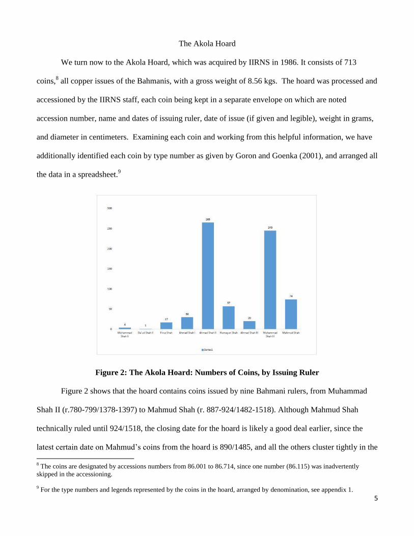
Figure 2: The Akola Hoard: Numbers of Coins, by Issuing Ruler
Figure 2 shows that the hoard contains coins issued by nine Bahmani rulers, from Muhammad
Shah II (r.780-799/1378-1397) to Mahmud Shah (r. 887-924/1482-1518). Although Mahmud Shah
technically ruled until 924/1518, the closing date for the hoard is likely a good deal earlier, since the
latest certain date on Mahmud’s coins from the hoard is 890/1485, and all the others cluster tightly in the
8 The coins are designated by accessions numbers from 86.001 to 86.714, since one number (86.115) was inadvertently
skipped in the accessioning.
9 For the type numbers and legends represented by the coins in the hoard, arranged by denomination, see appendix 1.

6
early years of his reign—four coins dated to 887, and one each to 888, 889, 88[x] and 89[x]. If the third
digit in the last date is 9, then the closing date could be as late as 899/1493; if it is zero, then it would
work out to 890/1485.10
In any case, the hoard includes coins that were minted over a period of
approximately one century. The coins of Ahmad Shah II (r.1436-1458) are the most numerous—265—
followed by those of Muhammad Shah III (r.1463-1482) as a close second, with 245 coins. The coins of
the earliest rulers in the hoard are the smallest in number, and understandably so, since the numbers of
those coins still in circulation a century later at the closing date of the hoard must have fallen off
dramatically thanks to the processes of loss, hoarding, and official withdrawal of damaged and heavily
worn coins.
Māṣas #coins Percentage
18 342 48.0%
12 161 22.6%
9 172 24.1%
6 38 5.3%
TOTAL 713 100%
Fig. 3: Numbers and Percentages of denominations in Akola Hoard
The hoard contained coins of four different sizes, belonging to the 6-, 9-, 12-, and 18-māṣa
denominations mentioned in the previous section. Their relative numbers were such that there seems to
have been a preference for the highest denominations on the part of whoever it was who assembled the
hoard. As figure 3 shows, the 18-māṣa denominations account for nearly half of the contents of the
hoard (342 coins or 48%), the 12 and 9 māṣa coins account for about a quarter each (161 coins or 22.6%
and 172 coins or 24.1%), and the 6 māṣa coins only a small fraction of the hoard (38 coins or 5.3%).
How the relative proportions between the denominations changed in the coins of each issuing ruler is
shown in figure 4. The coins of the first three rulers included only 6-māṣa denominations; 9-māṣa
coins first appear in the coins of Ahmad Shah I, as do also 18-māṣa coins, although more tentatively.
But in the reign of his successor Ahmad Shah II, the 12-māṣa denomination first appears, and the 18-
10
For the regression analyses presented later in the essay, we chose the date of 892/1486 as the closing date for the hoard, for
reasons explained below (see page 18).

7
māṣa denomination continues to grow at the expense of the smaller denominations, until it accounts for
nearly 2/3rds of all the coins issued by the last four rulers.
Figure 4: The Akola Hoard: Percentages of denominations by ruler
Using Denominations
At this point, it will be useful to think more explicitly about denomination sets, and how the
ways in which they are structured enable certain types of monetary activity that would not be possible
otherwise.11
To this end, figure 5 presents the data of the hoard in yet another way, in the form of a
frequency graph plotting the numbers of coins against weights (at 0.2 g intervals). The resulting
histogram shows that the coins are tightly concentrated within four compact weight ranges, and that
these are separated from each other by clear gaps with no coins in the intermediate ranges. (The sole
exception is the anomalous coin at the 13 g mark, to which we will return below.) This tight clustering
has implications that are simple but important: it permits coins that fall within the same narrow weight
11
The term “denomination set” is borrowed from Robert Tye, who rightly states that from the perspective of social and
economic history, “the appropriate unit of study should be the set of denominations available at a specific time, to a specific
population.” See Robert Tye, Early World Coins and Early Weight Standards (York: Early World Coins, 2009), p. 104.

8
range—even if they are in fact slightly different in size and weight—to be seen and treated as the same,
and at the same time, to be seen as different from coins falling within adjacent ranges. This enables users
of the currency to quickly identify, sort, and count out a certain number of coins within a given range in
order to make a payment for some commodity. And they are able to do this on the basis of simple visual
criteria—registering the relative diameter and thickness of the coins—and then confirming that
judgement in a tactile manner by feeling the relative weights of the coins (fig. 6). There is no need for
the coins to carry a number or name identifying their denomination, nor is it necessary for the ordinary
user to be able to read Persian and decipher the multiple names and titles occurring on the different
denominations.12
Figure 5: The Akola Hoard: frequency of coin weights showing denominational structure
12
This is an important point—that recognition of the denomination does not depend on reading the legend—since each ruler
differentiated his coins at a given denomination from those of his predecessors by varying the titles employed, and some
rulers, most notably Mahmud Shah, issued certain denominations with legends of up to four different types. Indeed, if
knowledge of the legends were a crucial component of the ability to recognize denominations, a user of the Bahmani copper
currency would have needed to carry a mental catalogue of 28 different legends in order to identify the four denominations
(see Appendix 1). But there would have been no need for anyone to do this—other than moneychangers and workers at the
mint—since the direct physical properties of the denominations are such that the coins of different values can be easily
distinguished—as the photograph in figure 6 clearly suggests.

9
There is an additional point of importance that emerges from inspection of this histogram. Each
of the four weight ranges begins immediately to the left of the māṣa value that Marie Martin has taken
as defining that denomination metrologically, represented by the four vertical lines inscribed at its gram
equivalent on the weight axis of the histogram.13
This suggests that the māṣa values of the four
denominations—18, 12, 9, and 6—were taken as the nominal mint weights for their respective
denominations, and that any coin falling into the weight range just to the left of one of these nominal
mint weights—let us say, the 18-māṣa denomination—would be considered an 18-māṣa coin regardless
of how much lighter it weighed, so long as it fell within the accepted range. Using these nominal values
rather than the actual weights of the coins would have ensured that it was still possible to make use of
the natural proportionate relationships obtaining between the denominations. For example, it would
have been possible to pay for something with a price of 18 māṣas with two 9-māṣa coins, even if the
total of their two weights did not quite add up to a full 16.52 grams.
The points made in the paragraphs above can be made still clearer with two contrasting examples
taken from two very different currency systems, neither of which bothered to strike coins within
narrowly constrained weight limits, as the Bahmanis did. The first example is provided by the reform
coinage minted by the Byzantine emperor Anastasius in 498 CE, based on the copper follis of 40 nummi,
13
See note 7 above.
Fig. 6: A stack of Bahmani copper coins:
6-mashas
9-mashas
12-mashas
18-mashas
10
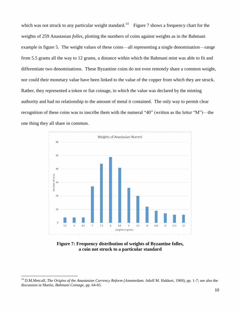
which was not struck to any particular weight standard.14
Figure 7 shows a frequency chart for the
weights of 259 Anastasian folles, plotting the numbers of coins against weights as in the Bahmani
example in figure 5. The weight values of these coins—all representing a single denomination—range
from 5.5 grams all the way to 12 grams, a distance within which the Bahmani mint was able to fit and
differentiate two denominations. These Byzantine coins do not even remotely share a common weight,
nor could their monetary value have been linked to the value of the copper from which they are struck.
Rather, they represented a token or fiat coinage, in which the value was declared by the minting
authority and had no relationship to the amount of metal it contained. The only way to permit clear
recognition of these coins was to inscribe them with the numeral “40” (written as the letter “M”)—the
one thing they all share in common.
Figure 7: Frequency distribution of weights of Byzantine folles,
a coin not struck to a particular standard
14
D.M.Metcalf, The Origins of the Anastasian Currency Reform (Amsterdam: Adolf M. Hakkert, 1969), pp. 1-7; see also the
discussion in Martin, Bahmani Coinage, pp. 64-65.

11
The second example is provided by Ghaznavid gold and silver coinage, which similarly was not
minted to a strict weight standard. But this was not because it was a token coinage—to the contrary, it
was a commodity coinage with its value based on that of the gold or silver it contained—but rather,
because it passed not by count (tale) but by weight. In other words, the legend with which each coin
was struck guaranteed the metal’s purity, but not the amount of the metal it contained; in order to
calculate the value of a given number of coins, it would have been necessary to weigh them out with a
balance.15
These contrasting examples permit us to draw two conclusions about the Bahmani copper
currency. First, the coinage must have been accepted by count, because there seems to be no other
reasonable explanation for why the mint authorities would go to such trouble to mint the coins to so
narrow a weight margin, and to separate the denominations by such carefully maintained intervals, if
they were still to be weighed before each transaction. Striking according to such narrowly defined
denominations can only have been for the purpose of making the coinage easier for ordinary people to
use in market transactions. Second, the coinage must have functioned as something in between a
commodity coinage, based on the value of its copper, and a token or “fiat” coinage with its value
determined by the state and unrelated to the amount of copper it contained. If it had been purely a fiat
coinage, then there would have been no reason to use more copper to make the higher denominations
larger and heavier; instead, it would have been possible to mint all four denominations at the same size
and then to differentiate them solely by means of numbers, in a manner akin to the Byzantine folles, but
inverted (i.e., multiple numbers to differentiate identically sized coins, instead of, as with the folles, a
single number to identify differently sized coins). On the other hand, it seems likely that the coins would
have carried a small and variable amount of additional value over that of the amount of copper they
contain, in effect guaranteeing that the lower weight coins would still carry a value equal to that of a
15
Deyell, Living without Silver, p. 73.
12
coin realizing the ideal mint weight. For this type of coinage, we may use the term “fiduciary” coinage,
as employed by Sargent and Velde.16
Interpreting the Bahmani copper coinage as a fiduciary coinage additionally helps make sense of
the weight distributions in the denominational frequency chart. Any coin with a weight above the
nominal mint weight for that denomination, would be, by definition, more valuable as a piece of copper
than as a piece of money, creating an incentive for it to be taken out of circulation, melted, and restruck
to a weight below the nominal mint weight. Conversely, with underweight coins, there would be no such
incentive until one came to the most heavily underweight coins, at which point it would be expedient to
take them back to the mint or moneychanger in exchange for coins within the expected normal weight
range. This would account for the steeper slope of the weight distribution curve on the right side (higher
weight values) and the more gradually tapering distribution curve on the left.
In this connection, we may recall that in the case of the 18 māṣa denomination, there was one
unusually lightweight outlier located half way between the 18 and 12 māṣa distributions.
Typologically—even if not by weight—this coin is an 18-māṣa specimen, but it is so light that one
would expect it to have been taken out of circulation instead of ending up in this hoard. One suspects
that had the coins in the hoard remained in circulation, the next time a moneychanger spotted that coin,
it would have been culled and returned to the mint, since it would have been too ambiguous for the
ordinary money user to decide whether it was supposed to be an 18- or a 12-māṣa coin.
To recapitulate the points made in this section, the Bahmanis’ use of multiple, clearly
differentiated denominations of copper coins would have had three related implications for how the
money was used:
16
Sargent and Velde define “fiduciary” money as that which is “overvalued”, that is, taken for more than its intrinsic value.
See Thomas J. Sargent and Francois R. Velde, The Big Problem of Small Change (Princeton: Princeton University Press,
2002), p. 375.

13
1) First, the tight clustering of individual coin weights within narrow denominational bands
separated by clearly defined gaps would have facilitated visual and tactile recognition, sorting,
and counting of the coins. This means that the coins could pass by count, instead of by weight,
and that there would accordingly be no need for an intermediary with a balance to be interposed
between buyer and seller.
2) The establishment of a fiduciary coinage, in which the coins carried a value somewhat greater
than that of the copper they contained, made it possible for people to use underweight as well as
full-weight coins, so long as they fell within the acceptable weight range for that denomination,
and to refer to them equally with the nominal denominational value. This would have alleviated
any qualms about wear having a negative effect on the coins’ value.
3) The minting in a range of denominations, all expressed in terms of numbers of māṣas
exhibiting natural proportional relationships with each other, would have facilitated handling the
money, making payments, and making change. For example, if one were going to the bazaar to
make a more substantial purchase with the value of 180 māṣas, it would make more sense to
carry the sum as ten 18-māṣa coins, rather than as thirty 6-māṣa coins. Even though both sums
would weigh approximately the same amount, and carry exactly the same value, it is far easier to
count and keep track of 10 coins than it is of 30.
In sum, the analysis of the Akola hoard thus far suggests that the multi-denominational copper coinage it
contained would have had the effect of facilitating and encouraging monetary transactions at the non-
elite level.
Circulation and Weight Loss

14
Thus far, we have considered the Akola hoard synchronically, that is, as providing a glimpse into
the workings of the Bahmani monetary system at a particular moment in time early in Mahmud Shah’s
reign, in about 1485-93, at which point the hoard was closed and deposited. Thus, each of the
denomination distributions in figure 5 represents not only the coins that were minted at the end of the
fifteenth century by Mahmud Shah, but also those of the same denomination issued by any of his
predecessors who also minted that denomination. Yet, these are all amalgamated and not distinguished
from one another. At this point it will be worthwhile to disaggregate the data for these different regnal
periods so we can analyze them diachronically and gain a better sense of how the coinage changed over
time. Here the most relevant factor to consider is weight loss, as this can reveal much about the velocity
at which coins have circulated, which can in turn reflect the degree of monetization within a society.17
As D.D.Kosambi has demonstrated experimentally, populations of coins of a single type that
have been minted to a common weight standard and put into circulation at the same time will exhibit
two characteristics over time. First, their average weight will decrease due to the slow wearing away of
metal through handling and exchange, and second, the spread between their lowest and highest weights
will increase since some coins will inevitably experience more vigorous circulation (the lower weights)
and others will see less (the higher ones). Visually, this can be expressed in a frequency chart, with
weights on the x-axis and numbers of occurrences on the y-axis. The frequency distribution of the coin
weights at the time of minting would have a high and narrow peak, theoretically centered over the ideal
minting weight, and sides that fall off steeply. After they have circulated for some time, a distribution
curve of the same coins would not only have shifted to the left (as their average weight declined) but
17
There is of course no simple and direct link between velocity of circulation and the degree of monetization. Indeed,
Nicholas Mayhew has recently called attention to the “counter-intuitive truth” that “velocity falls as one moves towards more
modern times, even though it is clear that the use of money has generally become more and more prevalent over time…
Increasing dependence on the use of money in society called for ever greater supplies of money, since all of us need to hold
quantities of cash idle in readiness, if it is to be available at the moment when we choose to spend it. Thus Velocity falls the
more we depend on the use of money (Nicholas Mayhew, “The President’s Address, 19 June 2012: The Quantity Theory of
Money: 3. Velocity”, The Numismatic Chronicle 172(2012):397-403). Moreover, as Lockyear has noted, studies of relative
monetization “have generally been hampered by a lack of definition” (Lockyear, Multivariate Money, p. 55). But we would
agree with his cautious acknowledgement that “speed of coin circulation could still be a useful parameter to chart as it should
partly reflect the uses to which coinage was put, and perhaps the degree of ‘monetization’ of an economy” (p.267-8).

15
also flattened at the same time, covering a greater range of different weights due to the differential
effects of wear.18
Figure 9: Weight loss in 18-māṣa denominations issued by five successive rulers over a period of
57 years: Ahmad II (1436-1458) to Mahmud (1482-1493)
Can we observe these characteristics—leftward shift and flattening of the curve—if we graph the
distribution curves for the coins of a single denomination as minted by different rulers represented in the
Akola Hoard? Figure 9 presents such a graph, showing the 18-māṣa weight and number distributions
for 5 consecutive rulers. Although there is little to differentiate the three most recent rulers (moving
backwards in time, Mahmud, Muhammad III, and Ahmad III, covering a span of approximately 30
years), there is a significant difference between their curves and those of the two earliest rulers,
Humayun and Ahmad II, whose outputs covered the previous 25 years. In their cases, not only has the
peak shifted to the left, but it has also been brought down lower than the peaks of the other three rulers,
and is spread out more widely. What this means is that after being in circulation for only an additional
25 years, these coins vividly show the effects of wear.
18
D.D. Kosambi, “The effect of circulation upon the weight of metal currency,” Current Science XI (1942): 227-31, and
“Scientific Numismatics,” Scientific American (Feb. 1966): 102-111. Both articles have been reprinted in D.D.Kosambi,
Indian Numismatics, New Delhi: Orient Longman, 1981.

16
It is one thing to say that the coins show weight loss, and yet another to be able to talk about that
weight loss in a quantifiable manner. A simple way to do so would be to look at what is happening to the
average weight of the coins in any particular denomination for earlier and earlier reigns. If wear is taking
place, we would expect the average weight of the coins of a particular denomination to be lower for
earlier reigns. Further, if the distribution of weights is flattening and moving to the left, we would expect
the mode (the weight at which the distribution is at its highest, indicating the “most common” weight) to
also be shifting to the left, but not so much as the mean weight which moves farther to the left due to the
skewing of weights toward that direction. Figure 10 presents this data in the form of a table. In the table,
the reigns are listed in chronological order, with later reigns occupying columns further to the right. For
each denomination and for each reign, we provide the number of coins (n), the mean weight and the
modal weight. We see that, except in cases where the number of coins in a category is so small that the
sample could easily be non-representative, the average and modal weights decline with age and the
mode remains to the right of the mean.
18-māṣas Ruler Ahmad II Humayun Ahmad III Muhammad III Mahmud
n 98 34 12 151 43
Mean 15.67 15.68 15.97 15.89 15.90
Mode 15.8 15.8 16 16 16
12-māṣas Ruler Ahmad II Humayun Ahmad III Muhammad III Mahmud
n 55 18 4 58 26
Mean 10.33 10.33 10.37 10.56 10.56
Mode 10.4 10.4 10.5 10.6 10.6
9-māṣas Ruler Ahmad I Ahmad II Humayun Ahmad III Muhammad III Mahmud
n 17 112 3 4 31 5
Mean 7.57 7.63 7.60 7.73 7.77 7.86
Mode 7.7 7.8 7.67 7.8 7.8 7.8
6-māṣas Ruler Muhammad I Da’ud II Firuz Ahmad I Humayun Muhammad III
n 4 1 17 9 2 5
Mean 4.65 4.64 4.70 4.82 4.91 5.14
Mode 4.75 4.8 4.8 4.8 5 5.2
Figure 10: Mean and Mode of Coin Weights, by ruler and denomination

17
A more formal way to quantify the weight loss phenomenon would be to run ordinary least
square regressions on the data. Say we postulate a very simple process, that a coin loses, on average, a
fixed, but unknown, proportion of its weight every year.19
Of course this is over-simplified, but we are
dealing with averages. Under this assumption, the weight of a coin in year 1 (𝑤1), one year after it was
minted, could be represented as
𝑤1 = 𝜃𝑤0
where 𝑤0 is the (unknown) weight in year 0 (the year the coin was minted), and θ is the fraction of the
weight remaining after the weight loss. If there is no weight loss, 𝜃 = 1; otherwise, it is a number less
than 1 (say 0.99 if the weight loss is 1% per year). The weight loss factor, i.e., the fraction of weight that
is lost each year, is (1 − 𝜃).
Following this process, in year 2 the weight would be
𝑤2 = 𝜃𝑤1 = 𝜃2𝑤0
in year 3, it would be
𝑤3 = 𝜃𝑤2 = 𝜃3𝑤0
and so on; so that in year t the weight would be
𝑤𝑡 = 𝜃𝑡𝑤0.
Since this equation is not linear, we cannot apply linear regression techniques to it. However, it can be
converted to a linear equation by a simple transformation: taking natural logarithms. Explaining what
exactly a natural logarithm is would be difficult as it is quite technical and would take us too far off-
subject; suffice it to say that this is a transformation that converts the exponential equation above into a
linear one. The logarithmic transform of this equation is:
ln 𝑤𝑡 = 𝑡 ln 𝜃 + ln 𝑤0.
19
This assumption goes against the finding of Cope that the rate of wear of copper pennies in modern times increases over
time, perhaps because there is a constant loss of thickness over time. However, a glance at the scatter diagrams in the
Appendix, showing the relationship between age and weight of the coins in the hoard does not indicate this at all. The
interested reader can look at the contrast between our scatter diagrams and Cope’s to be convinced that his result does not
apply to this medieval coinage. See R. G. Cope: “The Wear of U.K. Coins in Circulation,” Wear 13 (1969), pp. 217-224.

18
We may rearrange this equation in the form
ln 𝑤𝑡 = ln 𝑤0 + (ln 𝜃) 𝑡.
This is a linear equation of the familiar form
𝑦𝑡 = 𝑎 + 𝑏𝑥𝑡.
Here, our dependent variable 𝑦𝑡 is the natural logarithm of the weight of a coin (ln 𝑤𝑡), the independent
variable 𝑥𝑡 is the age of the coin (𝑡), the coefficient of the independent variable 𝑡 in the regression, 𝑏, is
the natural logarithm of one minus the weight loss factor (ln 𝜃), and the intercept 𝑎 is the natural
logarithm of the weight of the coin at the time of its minting (ln 𝑤0).
Now of course the age of a coin is not the only factor that determines its weight. Hand-struck
coins would not have weighed the same at the time of minting, some coins might have been used much
more often than others (and therefore worn more), and so on. As is customary, in order to render the
equation amenable to the application of linear regression techniques, we rewrite it in the form
𝑦𝑡 = 𝑎 + 𝑏𝑥𝑡 + 𝜖𝑡
where 𝜖𝑡 is the random error term, meant to capture all the other factors that would have affected the
observed weight of the coin and assumed as usual to have a mean of zero and a variance 𝜎𝜖2.
In running the regressions, we expect under the theory of weight loss that the regression
coefficient b (or ln 𝜃) would be negative, indicating that weight declines with the age of a coin. As a
bonus, the regression for any denomination would yield an estimate of the average weight at time of
minting 𝑤0, since ln 𝑤0 is the intercept of the regression.
We of course had the weight of every coin in the hoard. For the closing date of the hoard, we
selected the year AH 892/1486 CE, although in reality the closing date could be any year in between 890
and 898, because the last digit of the coin bearing this date is not legible. But since we need a fixed
closing date in order to calculate the age of each coin in the hoard at the time of the hoard’s closing, we
chose 892 which appears to be a likely possibility given the other documented dates for the hoard’s

19
coins issued by the last ruler, Mahmud Shah.20
When the date of a coin was legible on the coin itself, we
calculated its age by taking the difference between 892 and the date on the coin. There were 156 coins
(out of the 713 in the hoard) for which the date was fully legible. There were additionally 74 coins for
which the date was only partially visible, the last digit being illegible. In these cases, we took the date to
be the mid-point of the decade if the sultan ruled throughout the decade, or the mid-point of that portion
of the decade under the sultan’s rule if he ruled for only part of it. Finally, when not enough of any date
was visible on the coin, we took its date to be the mid-point of that sultan’s reign and calculated the age
accordingly.
We ran four regressions, one for each denomination. Details of the results are presented in
Appendix II, but the main results are summarized in Figure 11. All the slope coefficients were negative
and statistically significant even at the 99% confidence level, giving powerful support to the weight loss
hypothesis. The P-values (probabilities of getting the results we did under the null hypothesis of no
weight loss)21
are all considerably below 1%. The highest P-value was for the 6-māṣa regression, and
even there it was a miniscule 0.006%, meaning that there was about a six-thousandth of 1% chance that
we found the slope we did even though there was no weight loss. In short, it is virtually certain that our
data verify weight loss. These results are as definitive as we could have hoped for.
Figure 11 presents a summary of the key results. We see the calculated slope for each regression
in the first row. The second row presents the P-values, on which we have already commented, and show
how strong the weight loss results are. The third row shows what the estimated slope tells us: the
estimated rate of weight loss per year. This varies from a low of 0.042% for the 18-māṣa coins to a high
of 0.120% for the 6-māṣa coins. The 12- and 9-māṣa denominations show weight loss in the 0.06% to
0.07% per year range. These numbers would indicate that the 6-māṣa coins circulated the most
vigorously, at least among the users of this hoard’s coins, while the 18-māṣa coins circulated the least
20
See the discussion on page 6. 21
The P-values are calculated based on an alternative hypothesis that the slope is less than zero (one-tailed test).

20
vigorously. That assumes that weight loss comes only, or at least primarily, from circulation, and that
the speed of weight loss indicates the vigor of circulation. It is possible, however, that other factors also
play a role in the speed of weight loss. For example, perhaps the slower speed of weight loss in the 18-
māṣa coins is partly a consequence of their heavier weight, as compared to, say, a 6-māṣa coin. One way
in which coins might lose weight is by striking against one another in a change purse or money bag. Just
as an SUV suffers less damage than a sub-compact car if the two collide, it is possible that a heavier
coin loses less weight from jostling against other coins than does a lighter coin. In any case, this
hypothetical jostling of coins in a purse or money bag may itself be considered a part of circulation, in
the sense that one needs to have coins accessible if they are to be used. If there is little likelihood of
their being used, there is correspondingly less chance that they will be jostling about. But, having noted
them, we will ignore these considerations.
Denominations
18 māṣas 12 māṣas 9 māṣas 6 māṣas
Slope -0.000424 -0.000676 -0.000596 -0.001204
P-value <0.0001% <0.0001% 0.0060% 0.0057%
Implied Rate of Annual Weight
Loss 0.042% 0.068% 0.060% 0.120%
Intercept 2.769847 2.362156 2.057977 1.645922
Implied Average Weight at Mint 15.96 gm 10.61 gm 7.83 gm 5.19 gm
“Ideal” Mint Weight 16.524 gm 11.016 gm 8.262 gm 5.508 gm
Implied Weight as Percent of Ideal 96.56% 96.35% 94.77% 94.15%
Figure 11: Summary of Key Regression Results
It is worth thinking about what the numbers on weight loss tell us about how vigorously coins
circulated in the Bahmani kingdom. Richard Duncan-Jones, in his landmark study of money in the

21
Roman Empire, found that the speed of weight loss for bronze sestertii was 0.18% per year.22
Assuming
that the “propensity to lose weight” was the same for Roman sestertii and Bahmani coppers, our results
indicate that the vigor of money circulation was not as great in the Bahmani Sultanate as in the Roman
economy, but it was nevertheless quite significant, with the 6-māṣa coins losing weight at the rate of
0.12% per year, two-thirds the rate found for Rome. Although the velocity at which the 6-māṣa coins
circulated was not quite as high as that of the Roman sestertii, these findings do suggest a society that
was relatively highly monetized, even if in some of its sectors other forms of exchange—such as barter
or gift giving—may have continued to be important. We should also note that the denomination that
circulated most vigorously, the 6 māṣa coin, was the smallest of the four Bahmani denominations and
thus would have been the most accessible and useful coin for the least wealthy inhabitants of the
Bahmani realm. This suggests that even the urban poor and lower middle classes would have been able
to participate in the cash economy, reinforcing the points about non-elite coinage use made at the end of
the previous section.
On the Relationship between Actual Mint-weight and Nominal Mint-weight
We have observed above that in the Akola hoard, the weights of the coins in each of the four
denominations fall uniformly to the left of the nominal weights for their respective denominations. This
raises the question of how we are to understand the relationship between the nominal weight in māṣas
and the actual weight that the mint workers were striving to realize in minting those coins. Here too the
regression results provide us with some useful data. The last four rows in figure 11 show the results for
the intercept term of the regressions. Since the intercept is the natural logarithm of the average initial
(mint) weight of the coins, it needs to be converted to give that average weight at the time of minting.
The last two rows show how the estimated mint weights from the regressions compare to the “nominal”
22
Richard Duncan-Jones: Money and Government in the Roman Empire, Cambridge: Cambridge University Press, p. 191.
During the period of the Empire, the sestertius was a large “bronze” or copper coin weighing about 15 grams. It is thus
closely comparable in size to the the 18 masha Bahmani coin.

22
mint weight. We see that all the estimated mint weights are quite short of the nominal mint weights. The
fact that the regressions yield these estimates of the average weight at the time of minting is a real bonus
and benefit of the regression approach.
Of course, a more direct approach to find the average weight at time of minting would be to
actually look at coins as they came out of the mint and to weigh them. Since we do not have the
possibility of doing that, what we could do is to take the newest coins in each denomination and look at
their weights. This would yield a close approximation to the average weight at time of minting, since
these coins have not circulated that much. Looking at a number of “new” coins would also give us an
idea of the distribution of the weights of newly minted coins. In the hoard, the newest coins would be
those of Mahmud Shah, since the closing date of AH 892 implies that the hoard was buried relatively
early in his reign (AH 886-923). So we took the coins of Mahmud Shah in each denomination (there
were no 6-māṣa coins of Mahmud, so we had to leave that denomination out of this exercise) and looked
at their average weight and distribution.
Denomination Average Weight of
Mahmud’s Coins
Regression Estimate
of Mint Weight
“Nominal” Mint
Weight
18 māṣas 15.90 gm 15.96 gm 16.524 gm
12-māṣas 10.56 gm 10.61 gm 11.016 gm
9-māṣas 7.86 gm 7.83 gm 8.262 gm
Figure 12: Average Weights of Mahmud Shah’s Coins, Compared to Regression Estimates and the
“Nominal” Mint Weights
Figure 12 presents the average weight of Mahmud Shah’s coins (the “new” coins), compared to
the regression estimates of the average mint weight and the “nominal” mint weight. We see that the
average weights of Mahmud’s coins are very close to the regression estimates and quite far from the
“nominal” mint weights. Even more interesting are the distributions of the weights of Mahmud’s coins,
seen in Figure 13. We expected to see distributions that were skewed to the left, on the grounds that the

23
mint would avoid producing coins that were too heavy but would nonetheless be trying to reach the
“nominal” mint weight. On the contrary, the distributions are relatively symmetrical (except the 9-
māṣas, which is skewed to the right but in any case is not to be trusted because it is based on only five
coins). Thus it appears that the mint was shooting for a weight well short of the nominal mint weight;
the distribution around that “target” low weight would then be more or less normal.
0.00%
5.00%
10.00%
15.00%
20.00%
25.00%
15.4 15.5 15.6 15.7 15.8 15.9 16 16.1 16.2 16.3 16.4
18-masha weights ex-mint (Average = 15.90 gm) Ideal weight = 16.524 gm
18-masha weights ex-mint (43 coins)
0.00%
10.00%
20.00%
30.00%
40.00%
10.4 10.5 10.6 10.7 10.8 10.9
12-masha weights ex-mint (Average = 10.56 gm) Ideal mint weight = 11.016 gm
12-masha weights ex-mint (26 coins)

24
Figure 13: Distribution of the Weights of Mahmud Shah’s Coins
One last item we look at in the context of the weight at time of minting is John Deyell’s practice
of estimating the mint weight by adding the standard deviation to the mean weight of the coins of a
particular type in a hoard. In his excellent survey of methods of hoard analysis,23
Deyell mentions that
“for convenience sake … the upper standard deviation (�̅� + s.d.) is taken as a good approximation of the
ideal minting weight of any coin type.” Deyell does not provide any theoretical justification for this
measure; it is an ad hoc approach meant to counter any tendency to use the heaviest coin in the hoard to
yield the estimate of the minted weight.
23
John Deyell: Living Without Silver, Appendix D.
0.00%
20.00%
40.00%
60.00%
80.00%
7.8 7.9 8 8.1
9-masha weights ex-mint (Average = 7.86 gm) Ideal mint weight = 8.262 gm
9-masha weights ex-mint (5 coins)

25
Denominations
18 māṣas 12 māṣas 9 māṣas 6 māṣas
“Nominal” Mint Weight 16.524 gm 11.016 gm 8.262 gm 5.508 gm
Regression Estimate of Mint
Weight 15.96 gm 10.61 gm 7.83 gm 5.19 gm
Average Weight of Hoard Coins 15.80 gm 10.45 gm 7.66 gm 4.79 gm
Standard Deviation 0.35 0.26 0.23 0.25
Deyell Measure of Mint Weight =
Average + Standard Deviation 16.15 gm 10.71 gm 7.88 gm 5.04 gm
Implied Regression Intercept24
2.782202 2.371026 2.064600 1.617743
Estimated Regression Intercept25
2.769847 2.362156 2.057977 1.645922
95% Confidence Interval 2.765429 –
2.774264
2.355439 –
2.368873
2.045624 –
2.070329
1.605799 –
1.686045
Figure 14: Comparison of Regression Estimate with Deyell’s Measure of Mint Weight
Figure 14 presents calculations of Deyell’s measures of mint weight for the four denominations
of coins in the Akola hoard and compares them to the regression estimates. The Deyell measure
performs remarkably well; it is closer in all cases to the regression estimate than to the “nominal” mint
weight. But, in statistical terms, its performance is mixed. In two out of the four cases (18-māṣas and 12-
māṣas), the Deyell measure lies outside the 95% confidence interval around the regression estimate of
the intercept. In other words, we would reject the null hypothesis that the true measure was the Deyell
measure. However, in the other two cases (9-māṣas and 6-māṣas), the Deyell measure lies within the
95% confidence interval, and so we would be unable to reject the hypothesis that the Deyell measure
was indeed the true measure. For an ad hoc measure with no real theoretical basis, that is a pretty good
24
The “Implied Regression Intercept” is that value of the intercept that would have given rise to Deyell’s measure of the mint
weight. We would like to see if this falls within the confidence interval of the actual regression intercept, which would mean
that Deyell’s measure was more or less consistent with our estimate. If the “Implied Intercept” falls outside the confidence
interval, we would say that, statistically speaking, Deyell’s measure was different from our estimate. 25
From Appendix II.

26
performance, but the mixed result underscores the benefit of our regression approach which yields
estimates that are grounded more scientifically.
What are we to make of the considerable difference between the estimated mint-weights (as
implied by the regression intercepts) and the nominal mint-weights in whole māṣas? There would
appear to be at least four possible ways to account for this discrepancy. Namely, we could conclude
that:
1) Martin was wrong and there was no correlation between Bahmani copper coin weights and
whole māṣa values; or that
2) There was a correlation, but it was based on a different value for the māṣa than that used either
by Martin or Deyell; or that
3) The gap between the nominal mint weights and the estimated mint weights might be accounted
for in terms of weight loss from chemical cleaning of the hoard;26
or that
4) We should think of the nominal mint weight not as an ideal target that the mint strove to attain,
but as a weight in whole māṣas slightly higher than the actual target weight so as to impute
more value to the coin than the copper it contained, thus adding a fiduciary element to minimize
the chances of the coins being melted down for their copper, while also preserving the natural
proportions between the weights of the various denominations.
We remain uncommitted on this matter, although the first possibility can almost certainly be ruled out in
view of the clear denominational structure exhibited by these coins. The second option might be a
possibility, although the amount of variance would likely be too small to account for the size of the gap.
The third possibility would appear plausible, although nothing is known about the cleaning of the hoard,
26
Deyell has written that on average, there is a 2% reduction in the gross weight of a hoard from cleaning (1990: 283).

27
which was evidently done before IIRNS acquired it. The fourth option appears highly plausible,
although in the end, it could well be that the discrepancy was produced by a combination of factors, such
as those in the last two possibilities.27
Conclusions
There are many things we might like to know about the Bahmani currency system that must
remain beyond our grasp, at least for the present, due to the dearth of contemporary written sources,
whether historiographic, documentary, or epigraphic. For example, we still do not know with any
certainty the contemporary names by which the copper denominations were known, nor do we have the
kind of information about wages, commodity prices, and metal exchange rates that is available for
Mughal north India, for example. Nonetheless, our materially based analysis of the Akola hoard does
permit us to draw several tentative conclusions about the nature of the Bahmani copper currency. These
are offered here in the hope that they may serve as a basis and point of departure for future studies as
more evidence becomes available, whether in the form of previously unknown literary sources or in the
form of more intact hoards.
1). From the clear, denominational structure witnessed by the coins in the hoard, and from the
fiduciary nature of the coinage—by virtue of which the coins carried slightly more value than
that of the copper they contained—it is clear that they would have passed by tale and not by
weight. This would have simplified purchasing and payment transactions, as there would
have been no need for a moneychanger (sarraf) to be interposed between buyer and seller.
27
There is a theoretical fifth possibility, that the distribution of minted coins was normally distributed around the nominal
mint weight, but that those coins which weighed more than the nominal mint weight were culled out as worth more than the
coin’s value. This would give rise to the issued coins all being lighter than the nominal weight and so naturally the average
weight of the issued coins would be below the nominal mint weight. However, we can reject this possibility because it would
imply a distribution of weights that would be highly skewed to the left, but the distribution of weights that we observe in
Figure 13 is bell-shaped. Thus it does seem that the target mint weight lies below the nominal mint weight.

28
2) The availability of four commonly available denominations, manifesting natural proportional
relationships with one another, would likewise have encouraged and facilitated cash
transactions. If prices were expressed in terms of the largest, 18-māṣa unit, then the 12-, 9-,
and 6-māṣa coins would have been available to serve as 2/3rds, half, and 1/3rd
fractional
units, facilitating the making of change or the buying of smaller amounts of a given
commodity.
3) The fact that the different denominations could be clearly distinguished by simple visual and
tactile criteria, without relying on written legends or identification in Persian, meant that the
coinage could not only serve the elite, but also those who were not literate in Persian,
whether because of their lower social status or their non-Muslim identity. This reliance on
visual and tactile means of differentiating the denominations would have encouraged non-
elite members of society to be drawn into the cash economy.
4) The weight-loss data generated by the regressions clearly indicate that the copper coins
circulated vigorously, enough for the smallest of them to lose up to 0.12% of their weight
through handling each year. This is a rate that is 2/3s that experienced annually by copper
sestertii in Imperial Rome, a period characterized by high monetization by pre-Industrial
standards. It is also significant that we see significant variation in the rates of weight loss,
suggesting that it was the smaller denominations that circulated most vigorously, and the
heaviest least vigorously, suggesting that the 18-māṣa coins were the ones more likely to
drop out of circulation as they were pressed into service as a medium for storing value (much
as in the Akola hoard, where 18-māṣa coins account for just under half of the hoard).

29
Appendix I: Coin types in the Akola Hoard and legends by denomination
6 mashas 6 different legends
Type (G&G) Ruler legend
BH 053 Muhammad Shah II O: Muhammad Mahmud
R: ‘Abd ma’bud
BH 058
Da’ud Shah I O: al-mu’ayyad bi nasr Allah
R: Da’ud Shah
BH 066 Firuz Shah O: rājī riḍwān muhaimanī
R: fīrūz shāh Bahmanī
BH 076 Ahmad Shah I O: al-manṣūr bi-naṣr Allāh al-mannān
R: abū’l-mughāzī aḥmad shāh al-sulṭān
BH 100 Humayun Shah O: dārā’ī nigāhbān
R: humāyūn shāh bin aḥmad shāh al-sulṭān
BH 117 Muhammad Shah III O: al-mu ‘taṣim billāh shams al-dunyā wa’l dīn
R: muḥammad shāh bin humāyū nshāh al-sulṭān
9 mashas 6 different legends
BH 074 Ahmad Shah I O: al-mu’ayyad bi naṣr Allāh al-malik al-hannān
R: abū’l-mughāzī Aḥmad Shah al-sulṭān
BH 087 Ahmad Shah II O: al-wāthiq bi-ta’yīd al-malik lālah [sic!] abū’l-muzaffar
R: Aḥmad shāh bin Aḥmad Shāh Bahmanshāh
BH 099 Humayun Shah O: al-mutawakkil alā karam Allāh al-hannān al-ghanī
R: humāyūnshāh bin aḥmad Shāh al-walī al-Bahmani
BH 106 Ahmad Shah III O: al-muṭi’ al-mannān bi-amr Allāh
R: abū’l-muzaffar aḥmad shāh al-sulṭān
BH 116 Muhammad Shah III O: al-mu ‘taṣim billāh shams al-dunyā wa’l dīn
R: muḥammad shāh bin humāyū nshāh al-sulṭān
BH 135 Mahmud Shah O: al-mutawakkil alā’llāh al-hannān al-mannān
R: maḥmūd shāh bin muḥammad shah al-sulṭān
12 mashas 8 different legends; 4 of them issued by same ruler (Mahmud)
BH 085 Ahmad Shah II O: al-mutawakkil alā’llāh al-ghanī
R: ‘alā’ al-dunyā wa’l-dīn Aḥmad Shāh bin Aḥmad Shāh al-sulṭān
BH 098 Humayun Shah O: al-mutawakkil alā’llāh al-qawī al-ghanī abū’l-mughāzi
R: ‘alā’ al-dunyā wa’l-dīn humāyūn shāh bin aḥmad shāh bin aḥmad
shāh al-walī al-bahmanī
BH 105 Ahmad Shah III O: al-rājī bi-ta’yīd al-raḥmān
R: abū’l-muzaffar aḥmad shāh al-sulṭān
BH 115 Muhammad Shah III O: al-mu ‘taṣim billāh shams al-dunyā wa’l dīn
R: muḥammad shāh bin humāyū nshāh al-sulṭān
BH 128 Mahmud Shah O: al-mutawakkil alā’llāh al-hannān al-mannān abū’l-mughāzī
R: maḥmūd shāh bin muḥammad shah al-sulṭān
BH 129 Mahmud Shah O: al-mutawakkil alā’llāh al-hannān al-mannān abū’l-mughāzī
R: maḥmūd shāh bin muḥammad shah al-Bahmanī
BH 130 Mahmud Shah O: al-mutawakkil alā’llāh al-hannān al-mannān
R: maḥmūd shāh bin muḥammad shah al-Bahmanī
BH 131 Mahmud Shah O: al-mutawakkil alā’llāh al-qawī al-ghanī
R: maḥmūd shāh bin muḥammad shah al-Bahmanī
BH 133 Mahmud Shah O: al-mutawakkil alā’llāh al-qawī al-ghanī
R: maḥmūd shāh bin muḥammad shah al-Bahmanī (same as above but
different arrangement)

30
18 mashas 7 different legends
BH 073 Ahmad Shah I O: al-mustawthiq billāh al-hannān al-mannān al-ghanī
R: al-sulṭān aḥmad shāh bin aḥmad bin al-ḥasan al-bahmanī
BH 084 Ahmad Shah II O: al-mu’taṣim bi-ḥail Allāh al-mannān sammī khalīl al-raḥmān abū’l-
muzaffar
R: ‘alā’ al-dunyā wa’l-dīn Aḥmad Shāh bin Aḥmad Shāh al-sulṭān
BH 097 Humayun Shah O: al-mutawakkil alā’llāh al-qawī al-ghanī abū’l-mughāzi
R: ‘alā’ al-dunyā wa’l-dīn humāyūn shāh bin aḥmad shāh bin aḥmad
shāh al-walī al-bahmanī
BH 104 Ahmad Shah III O: al-mustanṣir bi-naṣr Allāh al-qawī al-ghanī
R: aḥmad shāh bin humāyū nshāh al-bahmanī
BH 113 Muhammad Shah III O: al-mu ‘taṣim billāh shams al-dunyā wa’l dīn
R: muḥammad shāh bin humāyū nshāh al-sulṭān khallada mulkahu
BH 114 Muhammad Shah III O: al-mu ‘taṣim billāh shams al-dunyā wa’l dīn
R: muḥammad shāh bin humāyū nshāh al-sulṭān
BH 123 Mahmud Shah O: al-mutawakkil alā’llāh al-hannān al-mannān abū’l-mughāzī
R: maḥmūd shāh bin muḥammad shah al-sulṭān
Note that in three cases, coins of two or more different denominations share identical legends:
BH 97 (18-māṣa) and BH 98 (12-māṣa) (both issues of Humayun Shah)
BH 114 (18-māṣa), BH 115 (12-māṣa), BH 116 (9-māṣa), and BH 117 (6-māṣa) (all issues of Muhammad Shah III)
BH 123 (18-māṣa) and BH 128 (12-māṣa) (both issues of Mahmud Shah)

31
APPENDIX II
REGRESSION RESULTS
18-māṣas
Regression Statistics
Multiple R 0.2705
R Square 0.0732
Adjusted R Square 0.0705
Standard Error 0.0221
Observations 342
Coefficients Standard
Error t Stat P-value
Intercept 2.7698 0.0022 1233.2982 <0.0001
Slope -0.0004 0.0001 -5.1812 <0.0001
Intercept 2.7698 Implied weight at time of minting28 15.96 gm
Slope 0.00042 Implied annual rate of weight loss 0.042%
28
Since 𝑒2.7698 = 15.96.
12.00
12.50
13.00
13.50
14.00
14.50
15.00
15.50
16.00
16.50
17.00
0 10 20 30 40 50 60 70 80
Age of Coin (in years)
Weights of 18-mashas
Weights of 18-mashas Expon. (Weights of 18-mashas)

32
12 māṣas
Regression Statistics
Multiple R 0.3992
R Square 0.1594
Adjusted R Square 0.1541
Standard Error 0.0230
Observations 161
Coefficients Standard
Error t Stat P-value
Intercept 2.3622 0.0034 694.5855 <0.0001
Slope -0.0007 0.0001 -5.4904 <0.0001
Intercept 2.3622 Implied weight at time of minting 10.61 gm
Slope -0.00078 Implied annual rate of weight loss 0.068%
9.00
9.50
10.00
10.50
11.00
11.50
0 10 20 30 40 50 60
Age of Coin (in years)
Weights of 12-mashas
Weights of 12-mashas Expon. (Weights of 12-mashas)

33
9 māṣas
Regression Statistics
Multiple R 0.2890
R Square 0.0835
Adjusted R Square 0.0781
Standard Error 0.0290
Observations 172
Coefficients
Standard Error t Stat P-value
Intercept 2.0580 0.0063 328.8815 <0.0001
Slope -0.0006 0.0002 -3.9354 <0.0001
Intercept 2.0580 Implied weight at time of minting 7.83 gm
Slope -0.0006 Implied annual rate of weight loss 0.060%
6.00
6.50
7.00
7.50
8.00
8.50
0 10 20 30 40 50 60 70 80
Age of Coin (in years)
Weights of 9-mashas
Weights of 9-mashas Expon. (Weights of 9-mashas)

34
6 māṣas
Regression Statistics
Multiple R 0.5854
R Square 0.3427
Adjusted R Square 0.3245
Standard Error 0.0430
Observations 38
Coefficients Standard
Error t Stat P-value
Intercept 1.6459 0.0198 83.1961 <0.0001
Slope -0.0012 0.0003 -4.3327 <0.0001
Intercept 1.6459 Implied weight at time of minting 5.19 gm
Slope -0.0012 Implied annual rate of weight loss 0.120%
4.00
4.20
4.40
4.60
4.80
5.00
5.20
5.40
0 20 40 60 80 100 120
Age of Coin (in years)
Weights of 6-mashas
Weights of 6-mashas Expon. (Weights of 6-mashas)