MOMENTUM AND MEAN REVERSION ACROSS NATIONAL EQUITY MARKETS*

RONALD J. BALVERS

Division of Economics and Finance College of Business

West Virginia University Morgantown, WV 26506-6025

rbalvers@wvu.edu Phone: (304) 293-7880, Fax: (304) 293-2233

and Tinbergen Institute

YANGRU WU

Department of Finance Rutgers Business School-Newark & New Brunswick

Rutgers University Newark, NJ 07102-3027

yangruwu@andromeda.rutgers.edu Phone: (973) 353-1146, Fax: (973) 353-1233

and Hong Kong Institute for Monetary Research

April 10, 2003 ABSTRACT A number of studies have separately identified mean reversion and momentum, but this paper considers these effects jointly: Potential for mean reversion and momentum is combined optimally into one indicator, interpretable as an expected return. Combination momentum-contrarian strategies, used to select from among 18 developed equity markets at a monthly frequency, outperform both pure momentum and pure contrarian strategies. Our key assumption is that, among developed markets, only global equity price index shocks can have permanent components, as would be reasonable in a production-based asset-pricing context, given that production levels converge across developed countries. The results are robust, reveal that it is important to control for mean reversion in exploiting momentum and vice versa, support an overreaction instead of an underreaction interpretation, and suggest that the “convergence hypothesis” is a fruitful one in the international asset pricing context. Keywords: Mean Reversion, Momentum, International Asset Pricing, Investment Strategies, Overreaction Hypothesis

* The authors thank seminar participants at Erasmus University, the Hong Kong Monetary Authority, Peking University, Rutgers University, West Virginia University, and PanAgora Asset Management, and Ivan Brick, Kai Li, Darius Palia and John Wald for helpful comments. Part of this work was completed while Balvers visited the Tinbergen Institute and Wu visited the Hong Kong Institute for Monetary Research. They thank these Institutes for their hospitality and financial support. The views expressed in this paper are those of the authors and do not necessarily reflect those of the Tinbergen Institute or the Hong Kong Institute for Monetary Research, its Council of Advisors or Board of Directors.

1

MOMENTUM AND MEAN REVERSION ACROSS

NATIONAL EQUITY MARKETS ABSTRACT

A number of studies have separately identified mean reversion and momentum, but this paper considers

these effects jointly: Potential for mean reversion and momentum is combined endogenously into one

indicator, interpretable as an expected return. Combination momentum-contrarian strategies, used to

select from among 18 developed equity markets at a monthly frequency, outperform both pure

momentum and pure contrarian strategies. Our key assumption is that, among developed markets, only

global equity price index shocks can have permanent components, as would be reasonable in a

production-based asset-pricing context, given that production levels converge across developed

countries. The results are robust, reveal that it is important to control for mean reversion in exploiting

momentum and vice versa, support an overreaction instead of an underreaction interpretation, and

suggest that the “convergence hypothesis” is a fruitful one in the international asset pricing context.

1

INTRODUCTION

Considerable evidence exists that both contrarian and momentum investment strategies produce excess

returns. The work of DeBondt and Thaler (1985, 1987), Chan (1988), Chopra, Lakonishok, and Ritter

(1992), Richards (1997), and others finds that a contrarian strategy of sorting (portfolios of) firms by

previous returns and holding those with the worst prior performance and shorting those with the best

prior performance generates positive excess returns. On the contrary, the work of Jegadeesh and Titman

(1993), Chan, Jegadeesh, and Lakonishok (1996), Rouwenhorst (1998), Chan, Hameed and Tong (2000),

Grundy and Martin (2001), Jegadeesh and Titman (2001), Lewellen (2002), and others reveals that a

momentum strategy of sorting (portfolios of) firms by previous returns and holding those with the best

prior performance and shorting those with the worst prior performance generates positive excess returns.

There is no direct contradiction in the profitability of both contrarian and momentum investment

strategies since contrarian strategies work for a sorting period ranging from 3 to 5 years prior and a

similar 3 to 5 years holding period, while momentum strategies typically work for a sorting period

ranging from 1 month (or more commonly 3 months) to 12 months and a similar 1 (or 3) to 12 months

holding period.1 The results correlate well with the findings of mean reversion at horizons of around 3 to

5 years and the findings of return continuation for horizons up to 12 months.2 Furthermore the

overreaction hypothesis of DeBondt and Thaler (1985, 1987), as formalized by DeLong et al. (1990,

1991), and the behavioral theories of Daniel, Hirshleifer, and Subrahmanyam (1998), Barberis, Shleifer,

and Vishny (1998), and Hong and Stein (1999) imply the observed pattern of momentum/continuation at

short horizons and mean reversion at long horizons.3 Of course, overreaction may also be generated in an

1 Lehmann (1990) and Jegadeesh (1990) find profitability of contrarian strategies for very short – 1 week to 1 month –periods. We refer to the horizon from one month to up to one year as “short” although some authors (for instance Lee and Swaminathan (2000)) refer to this horizon as “intermediate.” 2 For the early work on these issues, see for instance Lo and MacKinlay (1988), Fama and French (1988), and Poterba and Summers (1988). 3 Consistent use of terminology suggests that a process of mean reversion leads to profitable contrarian investment strategies; and a process of continuation leads to profitable momentum investment strategies. We prefer, however, the more common use of the term “momentum” to indicate both the process and the strategy.

2

efficient market when unanticipated persistent changes in risk or risk premia occur: when, say, a

persistent increase in systematic risk comes about, returns are initially low as information about higher

risk spreads but subsequently are higher as expected returns have increased due to the increased reward

for risk.

The purpose of this paper is to explore the implications of an investment strategy that considers

momentum potential and mean reversion potential jointly. Chan, Jegadeesh, and Lakonishok (1996,

p.1711) state prominently: “Spelling out the links between momentum strategies and contrarian strategies

remains an important area of research.” Subsequent research by Lee and Swaminathan (2000), and

Jegadeesh and Titman (2001) exploring these links confirms an earlier finding of Jegadeesh and Titman

(1993) that particular momentum-sorted portfolios experience eventual partial mean reversion. This

finding is important since it suggests that momentum and mean reversion, which in principle may occur

in different groups of assets, occur in the same group of assets—supporting the overreaction hypothesis

for this group of assets and rejecting existing equilibrium explanations of momentum as tied to risk (e.g.,

Johnson (2002) and Holden and Subrahmanyam (2002)). The reversal result, however, needs further

corroboration: it is established for U.S. data only; is weak in the 1982-1998 period; may not hold for

large firms after risk correction; and appears to be insignificant for prior losers (Jegadeesh and Titman

(2001)).

While it is essential to consider momentum and mean reversion effects jointly, traditional non-

parametric approaches make a combination strategy awkward. One could, for instance, construct a

portfolio of firms with a combination of high returns in the previous 1-12 months period and low returns

in the previous 3-5 years period, and buy this portfolio. One problem is: what should the holding period

be – 1-12 months or 3-5 years? More essential than the selection of a particular holding period is the

actual portfolio choice: how should an investor weigh the importance of momentum potential vis-à-vis

mean reversion potential?

We instead utilize the decomposition into permanent and transitory components from Fama and

French (1988) and employ a parametric approach, as in Jegadeesh (1990), Pesaran and Timmermann

(1995, 2000), and Balvers, Wu, and Gilliland (2000). Our decomposition assumes transitory price

3

components to be country-specific. To motivate this strong assumption, consider the context of a Lucas

(1978) production-based asset pricing model that relates asset returns to production growth. As

discussed in more detail in section IV, transitory differences in productivity then imply transitory

differences in stock price index levels. The transitory nature of shocks in relative production levels is

supported by the growth literature (see for instance, Baumol (1986), Dowrick and Nguyen (1989), and

Barro and Sala-i-Martin (1995)), which finds that “absolute convergence” occurs between developed

countries similar to those in our data set. More direct support for the transitory nature of cross-country

stock price index differences is based on our own estimation, which reveals that the rate of convergence

of industrial production across countries is quantitatively similar to the rate of convergence of equity

price indexes across these same countries.

Specific parameter estimates obtained under the assumption that cross-country price index shocks

are transitory allow construction of an expected returns indicator that naturally combines potential for

momentum and mean reversion into one number. Investing occurs at each point in time in the asset or

portfolio of assets with the highest indicator at that time (while shorting the assets with the lowest

indicator). The endogenous combination of the momentum and mean reversion potentials is in marked

contrast with non-parametric combination of forecasting variables. For instance, while no authors have

previously attempted to combine momentum and mean reversion potential, van der Hart, Slagter, and van

Dijk (2003) combine momentum and value potential in predicting excess returns across firms in

emerging national equity markets. They rank portfolios by the “score” obtained from adding with equal

weight the normalized value of a value measure to the normalized value of a momentum measure. But

there is no logical basis for determining the weights used in calculating the score.

Applying the parametric investment switching strategies to a sample of 18 developed national

equity markets we find that strategies combining momentum and mean reversion typically yield excess

returns of around 1.2 - 1.5 percent per month and generally outperform pure momentum and mean

reversion strategies, which in turn outperform a random-walk-based strategy. The results sustain the

view that full mean reversion occurs in all cases where momentum drives prices away from original

levels, thus siding with Jegadeesh and Titman (2001) and Lewellen (2002) in supporting the overreaction

4

perspective against the underreaction perspective of Conrad and Kaul (1998), Berk, Green, and Naik

(1999), Holden and Subrahmanyam (2002), and Johnson (2002). Accordingly, mean reversion

tendencies should be expected for all assets that display momentum, and we cannot think of some assets

being responsible for empirical findings of mean reversion with others responsible for momentum

findings.

Analytical decomposition of returns into momentum and mean reversion effects enables us to

identify how the effects are correlated. We find empirically a strong negative correlation of –34 percent,

implying that it is important to control for momentum when studying mean reversion and vice versa.

Momentum persists longer than previously found in isolation and mean reversion takes place quicker

than without controlling for momentum.

The outline of the paper is as follows. In section I we describe the model and a decomposition of

expected return into a common unconditional mean, the country-specific potential for mean reversion,

and the country-specific potential for momentum. Section II discusses the Morgan Stanley Capital

International (MSCI) data for the index returns in 18 developed equity markets over the 1970-1999

period and estimation issues. Basic results for pure and combination momentum with mean reversion

strategies and random-walk-based strategies are presented in Section III. Illustrative parameter estimates

and support for the convergence hypothesis are provided in Section IV and various robustness issues are

covered in Section V. Section VI concludes with an appraisal of the results and further discussion of the

implications.

I. THE MODEL AND A RETURN DECOMPOSITION

(a) An integrated mean reversion-momentum model

We adapt the model of Fama and French (1988) and Summers (1986) to apply in a global context

and to allow for momentum as well as mean reversion in equity prices. First define p it as the log of the

equity price index of country i with reinvested dividends, so that the continuously compounded return r it

is given as:

p - p = r i1-t

it

it . (1)

5

Superscripts everywhere indicate an individual country index.

Following Fama and French (1988), we separate equity prices into permanent and temporary

components. Empirically we consider portfolios for a homogeneous group of countries, which enables us

to add some structure to the model. Specifically we assume that any country-specific shocks are

transitory (i.e., stationary). The theoretical motivation for this important assumption is based on the idea

of “convergence.” Dowrick and Nguyen (1989) (see also Barro and Sala-i-Martin (1995), p.27) find that

real per capita GDP across the OECD countries displays absolute convergence, implying that real per

capita GDPs in these countries have a tendency to converge stochastically towards a similar level. This

would imply in the context of the Lucas (1978) asset-pricing model (see also Balvers, Cosimano, and

McDonald (1990)) that values of representative firms in these countries should converge as well. As our

sample consists of mainly OECD countries we expect the non-global components in equity prices in

these countries to be stationary.

For country i we have accordingly

x + y = p itt

it . (2)

The global price component is denoted by yt (which may have both permanent and transitory

components) and the country-specific component by xit (which is transitory). Further support for the

assumption of transitory country-specific price components is provided in Section IV.

Combining equations (1) and (2) yields:

it

ittt

it xx + y y = r 11 −− −− . (3a)

With enough countries i, and assuming that the global and country-specific components are uncorrelated,

we can set the average change in the country-specific component equal to zero. Thus:

1−− ttw

t y y = r . (3b)

where wtr denotes the worldwide average return. From equations (1)–(3) it is clear that

x x = r r i1-t

it

wt

it −− .

The temporary component x it is formulated quite generally to allow for both momentum and

mean reversion:

6

ηρδµδ it

ij - t

ij - t

ij

J

1=j

i1 - t

iiiit +x - x + x + = x )()1( 1−∑− . (4)

Equation (4) generalizes the Fama and French (1988) and Summers (1986) model by allowing the ijρ to

be non-zero, which captures the momentum effect. The constant µ i , the autoregressive coefficient iδ ,

the momentum coefficients ijρ , and the mean-zero normal random term η i

t (serially and cross-

sectionally uncorrelated with varianceση i2 ), can all vary by country.

Equations (1) - (4) represent an integrated mean reversion-momentum model. From these four

equations it is straightforward to find the return in country i as: 4

it

wj-t

ij-t

ij

J

1 =j

ii1-t

iwt

it r - r + x - 1 - r r ηρµδ +∑−=− )())(( . (5)

(b) Return decomposition

To simplify notation we redefine variables and use lag operators L j to write:

it

i-t

ii1-t

iit RL + X- 1 - = R ηρδ +1)()( , (6)

where wt

it

it rrR −≡ , ii

tit xX µ−≡ , and 1

1)( −

=∑≡ jJ

j

ij

i LL ρρ .

Or simply,

it

it

it

it MOM+ MRV= R η+ , (7)

with RL MOM X- 1 - MRV i-t

iit

i1-t

iit 1)(,)( ρδ ≡≡ .

The left-hand side of equation (7) represents the excess return for country index i (excess relative to the

world mean return). In obvious notation, the first term on the right-hand side represents the mean

reversion component of return and the second term on the right-hand side represents the momentum

4 Note that for empirical purposes i w t tr r− is directly observable in the data and that

1it

x−

can be identified from

11 1ii

tt typx −= −− −

(equation 2) plus the fact that 0 0ix = by construction of the MSCI data (all index values are set equal to

100 in December 1969). Thus, it x is generated as

1

ti i wt s s

sx r r= −∑

=. The iµ can be viewed as adjusting for the

measurement error introduced by the initialization error of setting 0 0ix = for each country i.

7

component of return.

The unconditional expectation of the mean reversion term )( itMRVE is equal to zero

(since ii1 - t = x E µ)( from equation (4)) and, similarly, the unconditional expectation of the momentum

component )( itMOME is equal to zero. Hence, average excess returns i

tR are zero and the realized

country returns itr can be cleanly decomposed into the global return w

tr , a mean reversion component, a

momentum component, and an idiosyncratic shock component. This formulation is flexible, yielding the

momentum formulation of Jegadeesh and Titman (1993) as a special case when iδ = 1 (for all i) and

iij ρρ = (for all i and j) and the mean reversion formulation of Balvers, Wu, and Gilliland (2000) as a

special case when ijρ = 0 (for all i and j).

In addition to generalizing the Fama and French (1988) model by allowing for momentum, we

deviate in two ways from their approach in the empirical implementation. Fama and French consider

returns information instead of price information. As first-differencing is accompanied by a loss in

information about slowly decaying processes (such as, typically, the mean reversion component) we

deviate from Fama and French by not differencing the data and focusing on price information instead of

returns information.5 The second deviation in the empirical implementation relative to Fama and French

(1988) is that, while we use time series information to estimate parameters as do Fama and French, we

take the additional step of assessing the usefulness of the parameter estimates in guiding trading

strategies. That is, we employ the parameter estimates (using only past information) for investment

decisions and evaluate the resulting excess returns.

The focus on investment strategies designed to exploit mean reversion and momentum is similar

to the DeBondt and Thaler (1985) approach designed to exploit mean reversion and the Jegadeesh and

Titman (1993) approach designed to exploit continuation, with the major difference that these approaches

are non-parametric whereas ours is explicitly parametric. For a similar parametric approach see

Jegadeesh (1990) and Balvers, Wu, and Gilliland (2000).

5 For an alternative approach that avoids first differencing while still utilizing earnings and cost of equity forecasts see

8

II. DATA AND ESTIMATION ISSUES

(a) Data

Monthly returns data are obtained from the MSCI equity market price indexes for a value-

weighted world average and 18 countries with well-developed equity markets: Australia, Austria,

Belgium, Canada, Denmark, France, Germany, Hong Kong, Italy, Japan, the Netherlands, Norway,

Singapore, Spain, Sweden, Switzerland, the United Kingdom, and the United States. We use here the

prices with reinvested gross dividends (that is, before withholding taxes; see Morgan Stanley Capital

International (1997) for details) converted to dollar terms. The period covered is from the start of the data

series, in December 1969, through December 1999. Table I shows the summary statistics, with average

monthly return and standard error for each country and each country’s beta with the world index return.6

(b) Estimation Issues

Estimation of our variant of the Fama-French permanent-transitory components model employs a

maximum likelihood estimation procedure. The model parameters to be estimated, in principle, are

the , the 2i ,i

ησδ iij µρ theand , the . This sums to a set of 18(J+3) parameters (where J represents the

number of momentum lags), which is a high number in light of our 18 by 361 panel. Hence, to improve

efficiency and avoid multicollinearity problems we set σσ ηη22 = i for all i and, in most specifications,

apply one or more of the following restrictions: δ δi = , iijj

ij ρρρρ == , (the iµ are always allowed to

differ by country as they allow for possible “mispricing” at the beginning of the sample period). Thus

anywhere between 21 and 18(J +2) +1 parameters remain to be estimated.

III. TRADING STRATEGY RETURNS

Lee, Myers, and Swaminathan (1999). 6 In principle, a comparison of the average returns by country allows us to check directly an unintended implication of our stylized model—that the (unconditional) mean returns are equal across countries. While it is easy to check from Table I that none of the average returns differ significantly from the world average return, we do not take seriously the view that mean returns are equal in all developed national markets. Rather we treat this as a simplifying assumption that is not essential for our results.

9

The joint consideration of momentum and mean reversion urges us to use a parametric procedure

for establishing the trading rules. We follow closely the parametric approach of Balvers, Wu, and

Gilliland (2000) who consider a strategy for exploiting mean reversion results, using only prior

information. Starting at 1/3 of their sample, they use rolling parameter estimates to obtain conditional

expected returns for the upcoming period and then buy the fund with the highest expected return and

short-sell the fund with the lowest expected return. We extend this strategy to exploit simultaneously the

mean reversion and the momentum effects. Accordingly, we employ a trading strategy of buying at each

point in time the country index with the highest conditional expected return and short-selling the country

index with the lowest conditional expected return, based on equation (5) and using parameters estimated

from prior data only. We start the forecast period at 1/3 of the sample, in January 1980, and update

parameter estimates as we roll the sample forward.

The empirical model of equation (5) is applied with 12 possible momentum lags and a one-month

holding period (or more if the latest available information does not induce a portfolio change) as the

baseline case. While six or nine lags are employed more commonly for exploring momentum effects, we

allow for additional lags because controlling for mean reversion can be expected to expose additional

momentum lags (at lags beyond nine or so, mean reversion that is not controlled for may mask the

presence of additional momentum lags). For the sake of comparison to existing approaches, we initially

also consider pure momentum and pure mean reversion strategies and related variations of the combined

momentum-mean reversion strategy. In Tables II-IV, we display four special cases based on equation (5):

the pure momentum model of Jegadeesh and Titman (1993), the pure mean reversion model of Balvers,

Wu, and Gilliland (2000), the random walk model (to be described below), and the simplest combination

mean reversion-momentum model. In these cases we report all reasonable variations in the sorting and

holding periods.

(a) Pure momentum strategies

We first replicate the momentum approach of Jegadeesh and Titman (1993) for our data set of

national equity market indexes. For the empirical model in equation (5) this is equivalent to setting iδ =

10

1 (for all i) and iij ρρ = (for all i and j); thus (excess) realized returns over the previous J sorting periods

are weighted equally in determining expected future returns. The country index with the highest expected

return (based fully on past momentum for this strategy) is chosen as the “Max1” portfolio and the country

index with the lowest expected return is chosen as the “Min1” portfolio. The strategy of buying Max1

and shorting Min1 and holding this portfolio for K periods is referred to as “Max1-Min1” and is listed

under the appropriate value for K (similarly “Max3” and “Min3” refer to the strategies of holding the

equally-weighted average of three country indexes with, respectively, the highest and lowest expected

returns).

Jegadeesh and Titman (1993) focus only on the permutations of J = 3, 6, 9, 12 and K = 3, 6, 9, 12

which are shaded in Table II. However, since our model is designed for forecasting returns one period

(month) ahead, we also add the case of K = 1, in which the portfolio is held only until the updated return

forecast is available. Additionally, we speculate that controlling for mean reversion as we do in our

combination model of equation (5) is likely to imply a longer duration of the momentum effect (since

positive momentum after, say, 12 months of previous momentum is likely to be offset by the downward

pull of mean reversion and thus would not register in a pure momentum approach). Accordingly we also

add the permutations for J = 15, 18, and K = 15, 18 in Table II.

The results for the period January 1980 – December 1999 (earlier data are reserved for parameter

estimation as is needed for other trading strategies) are displayed in Table II. These results generally

agree, both qualitatively and quantitatively, with those of Jegadeesh and Titman (1993) for U.S. equities

and those of Asness, Liew, and Stevens (1997), Rouwenhorst (1998) Chan, Hameed, and Tong (2000),

Griffin, Ji, and Martin (2002), and van der Hart, Slagter, and van Dijk (2003) for international equities.

Excess returns per gross dollar invested (net dollar investment is zero) for the Max1-Min1 and Max3-

Min3 portfolios are positive for all cases originally considered by Jegadeesh and Titman (shaded) and, in

the range most commonly considered, J = 6, 9 and K = 6, 9, equal to around 10 percent annually and

statistically significant for the Max3-Min3 cases. For the case of K = 1 returns are generally substantially

lower and sometimes negative which is consistent with Jegadeesh (1990) and Lehmann (1990). As

expected without controlling for mean reversion and consistent with Jegadeesh and Titman (2001),

11

excess returns for longer holding periods (K > 12) fall rapidly as K increases to 18. Additionally,

increasing the sorting period J beyond 12 months lowers returns substantially.

(b) Pure mean reversion and random walk strategies

A further special case of equation (5) arises if we ignore momentum and focus on mean reversion

only by setting ijρ = 0 (for all i and j). The resulting formulation is comparable to that used in Balvers,

Wu, and Gilliland (2000) to detect mean reversion, employing an international sample similar to ours.

Their approach requires employing all available (panel) data prior to the forecast period to estimate the

mean reversion parameter. Hence, in contrast to the momentum case in Table II we cannot vary J but we

can vary the holding period K as shown in Table III. Again, the results are consistent with those of

Balvers, Wu, and Gilliland and with the earlier work on contrarian strategies exploiting mean reversion

by DeBondt and Thaler (1985) and others. The contrarian strategy returns are positive in all cases. For

Max1-Min1 the excess returns rise with K to 11.1 percent at K = 6 and then slowly drop with K to 9.2

percent per annum for K = 18. The returns for Max3-Min3 are lower, increasing slowly from 3.4 percent

at K = 1 to 5.6 percent at K = 15 and then fall to 4.8 percent at K = 18. These results correspond

reasonably well to the results in Balvers, Wu, and Gilliland for annual data who find (for K = 12) the

Max1-Min1 return of 9.0 percent and the Max3-Min3 return of 8.4 percent.

Interestingly, the pure momentum Max1-Min1 strategy for the nine-month holding period (K =

9) taking J = 6, for instance, yields an annualized excess return of 9.3 percent (see Table II), whereas

over the same nine-month holding period the, ostensibly opposite, contrarian strategy based on pure

mean reversion yields an annualized excess return of 11.0 percent (See Table III). Thus, both momentum

strategies and mean reversion strategies can be profitable over the same holding period, but the

momentum strategy here considers only returns over the past six months while the mean reversion

strategy is predicated on the full return history. Note that, in principle, the two disparate strategies may

advocate identical portfolio holdings. In Section V we examine whether this is in fact the case.

Table III also shows the returns generated with a pure “random walk” strategy. This formulation

captures the essence of the strategy employed by Conrad and Kaul (1998). This strategy selects the

12

country index with the highest expected return obtained by averaging return realizations prior to each

forecast period. In a simple efficient markets view, as argued by Conrad and Kaul (1998), those assets

with the highest prior returns are likely to be riskiest and thus are expected to have the highest returns in

the future. Since all returns prior to the forecast period are used in obtaining the best estimate for

expected return, the sorting period J cannot vary (as is also true for the pure mean reversion case). Table

III reveals that this strategy produces negative excess returns, albeit statistically insignificant, for all

holding periods K. Clearly, this is an unexpected result given a simple standard efficient markets

perspective, but can be understood easily from a mean reversion perspective: higher past realized returns

likely indicate that future returns will be lower as equity prices return to trend. Note that the momentum

effect becomes unimportant here since, in contrast with the mean reversion effect, momentum carries

little weight in calculating the average return from all past data.

(c) Combination momentum and mean reversion strategies

We now present the returns obtained by following a strategy that, based on equation (5) and

using only prior information, combines the potential for mean reversion and momentum into one

indicator for each asset, and chooses for each period the asset with the highest expected return, Max1,

and shorts the asset with the lowest expected return, Min1 (and similarly for Max3 and Min3). Equation

(5) allows for eight basic ways of combining the potential for momentum and mean reversion into one

indicator, depending on whether the momentum parameters are allowed to differ by country and/or are

allowed to differ by lag and whether the mean reversion parameter is allowed to differ by country. We

take here as our baseline the most parsimonious case that encompasses both the pure momentum and pure

mean reversion cases, namely the case of one momentum parameter ( ρρ =ij for all i, and j) and one

mean reversion parameter ( δδ =i for all i). The returns for the seven alternative ways of combining

momentum and mean reversion are discussed in a robustness section (Section V).

Table IV displays the combination strategy returns based on equation (5) with one momentum

parameter and one mean reversion parameter. Excess returns are positive in all cases. For easy

comparison with the pure momentum case considered for the same permutations of K and J, the specific

13

instances in which the combination strategy outperforms the pure momentum strategy are shaded in

Table IV. There are 42 permutations of holding period K and sorting period J. In all 42 of 42

corresponding Max1-Min1 strategies and in 37 of 42 corresponding Max3-Min3 strategies, the

combination strategy outperforms the pure momentum strategy. The Max3-Min3 cases where the pure

momentum strategy works somewhat better are for J equal to 6 and 9 and K smaller or equal to 6. For the

16 cases considered by Jegadeesh and Titman (1993), shaded in Table II, the annualized average of the

pure momentum return for Max1-Min1 is 6.65 percent and for Max3-Min3 is 7.30 percent, while for

these same 16 cases the average combination momentum-mean reversion strategy return for Max1-Min1

is 11.05 percent and for Max3-Min3 is 8.84 percent (see Table IV).

Comparing the combination strategy return against the pure mean reversion return is more

difficult since sorting period J does not vary in the mean reversion case. Taking the average for the K =

3, 6, 9, 12 cases considered in Jegadeesh and Titman produces a pure mean reversion Max1-Min1 return

of 10.30 percent, only slightly lower than in the combination strategy case, but a pure mean reversion

Max3-Min3 return of 4.40 percent, less than half the combination strategy return.

A more relevant comparison, however, may be the comparison for the case of K = 1: since the

optimal forecast is updated each month, the most reasonable strategy for maximizing realized excess

returns is one where the portfolio, in principle, is adjusted each time when a new forecast is available.

This case of one holding period, given our parametric context, is the only variant that can plausibly be

motivated. The Max1-Min1 and Max3-Min3 returns for K = 1 increase with J until J = 9 or 12 before

diminishing, providing some indication that momentum effects last up to a year when controlling for

mean reversion, as opposed to the six to nine months typically considered. In the following, we use as

the baseline case the natural case of K = 1 and we set J = 12 to allow, in principle, for 12 possible

momentum lags. In this instance, the Max1-Min1 return is 9.5 percent under pure momentum, 8.5 percent

under pure mean reversion, and 16.7 percent under the combination strategy; the Max3-Min3 return is

11.2 percent under pure momentum, 3.4 percent under pure mean reversion, and 11.9 percent under the

combination strategy.

14

IV. ILLUSTRATIVE PARAMETER ESTIMATION RESULTS AND THE SPEED OF CONVERGENCE

(a) Parameter estimates for the baseline model and pure strategy models

To illustrate in detail the implications of considering momentum and mean reversion

simultaneously, we examine the parameters of the baseline combination model case. To review: the

baseline case of equation (5) sets δ δi = , ρρ =ij (for all countries i and lags j), and σσ ηη

22 = i , and

assumes a lag structure for the momentum effect with monthly lags up to 12 (J = 12). The latter is

suggested by the aforementioned literature on the momentum effect that finds momentum effects of

generally less than a year, together with the observation that controlling for mean reversion may increase

the estimated duration of the momentum effect. Additionally, the holding period is one month (K = 1) so

that for each period the zero-investment portfolio is chosen based on the best forecast for that period.

The pooled mean reversion parameter in the pure mean reversion case is estimated to be 0.9855

and the pooled momentum parameter in the pure momentum case is estimated to be 0.017 (not reported

in a table). For the pure mean reversion scenario, the half-life of the impulse is straightforwardly

calculated as ln(0.5)/ln(0.9855) = 47.46 months (slightly under four years); by nature the half-life for the

pure momentum case is not defined (infinite).

For the baseline momentum-with-mean-reversion case the parameter values are displayed in

Table V. The mean reversion coefficient δ pooled across countries equals 0.979 so that 1-δ, indicating the

speed of mean reversion, equals 0.021, the momentum parameter ρ pooled across lags and countries

equals 0.026; both the speed of mean reversion 1-δ and the strength of the momentum effect ρ are larger

than in the pure strategy cases. The variance of the idiosyncratic return shock ση2 pooled across

countries equals 0.0031. Quantitatively, these numbers imply that a cumulative return of 1 percent below

trend has a mean reversion effect on the expected return for the upcoming period of +0.021 percent. To

get an equivalent momentum effect, a returns shock of 0.81 (0.021/0.026) percent in the last 12 months

must occur. Alternatively, all else equal, if last period’s return is 1 percent higher, the expected return for

the upcoming month will be 0.026 – 0.021 = 0.005 percent higher; if the return 13 months ago is 1

15

percent higher, the expected return for the upcoming month will be 0.021 ⋅ 0.97912 = 0.016 percent lower.

Figures 1(1) through 1(3) shows the impulse response of the idiosyncratic part of the expected

price index level (for any of the countries) to a 10 percent shock in ηit , for the parameter values presented

above in the pure mean reversion, pure momentum, and baseline combination strategy cases. The half-

life for the combination strategy can be seen in Figure 1(1) to be around 40 months, although the mean

reversion component by itself implies a half-life of ln(0.5)/ln(0.979) = 32.66 months. The half-life for the

combination strategy is shorter than in the pure mean reversion case (shown in Figure 1(3)), in spite of

the momentum component, because its speed of mean reversion 1-δ is larger. Intuitively, with momentum

added in appropriately, several effects alter the calculation of the half-life. First, the continuation due to

the initial shock causes the downturn to start later (beyond the 12 months of momentum lags in the

baseline case) causing the half-life to be longer; second, as the downturn starts, the momentum effect

reinforces it, causing the half-life to be shorter. Note in both Figures 1(1) and 1(2) that the momentum

period is longer than the 12 momentum lags assumed. The reason is that, while the exogenous shock

directly affects the momentum component for 12 periods only, the endogenous momentum responses in

periods one through 12 imply that even in month 13 and beyond the momentum component may still be

positive and exceed the mean reversion component.

(b) Decomposition of return variance

Table V displays the R-squared for the expected return regression as 0.0262 so that only 2.62

percent of return variability is explained by the momentum and mean reversion components combined as

follows from equation (5). Hence, from month to month the model explains 2.62 percent of returns

variability. As Cochrane (2001, p.446) notes, however, even predictability of 0.25 percent would be

enough to explain the excess momentum returns generated in the empirical work of Jegadeesh and

Titman (1993) and others.7 Intuitively, while the predictable variation for the average asset (country

7 Numerically, following the computation in Cochrane (2001, p.447), multiply the standard deviation of the return (0.00315)1/2 by the standardized expected return of the asset in the top 18th of the standard normal distribution, 2.018 (obtained by finding the expected value of the standard normal variable over the interval from 1.594 to infinity), and this times the square root of the predictable variation (0.0262)1/2, yielding 0.0174 which is the expected monthly excess return; shorting the bottom 18th asset and annualizing implies an expected return of 43.8 percent. This number compares

16

index) is small, the predictable variation of an asset deliberately selected for the extreme values of its

forecasting variable is much larger.

Taking the variance in equation (7), given that 22and,, ηη σσρρδδ === iij

i for all i and j,

produces:

2),(2)()()( ησ+++= ttttt MOMMRVCovMOMVarMRVVarRVar . (8)

The variance consists of a part due to conditional variance 21 )( ησ=− tt RVar and a part due to changing the

prediction: ),(2)()()]([ 1 tttttt MOMMRVCovMOMVarMRVVarREVar ++=− .

The variance of the momentum component )( tMOMVar , averaged across countries, equals 5.215

⋅ 10-5, and the variance of the mean reversion component )( tMRVVar , averaged across countries, is

7.185 ⋅ 10-5. These numbers together with equation (7), in which both components tMRV and tMOM

count equally in calculating expected returns, imply that momentum and mean reversion are of similar

importance in affecting the combination strategy portfolio choices. Specifically, the ratio of the standard

deviation of the mean reversion component to the standard deviation of the momentum component is

(7.185/5.215)1/2 = 1.17, which can be interpreted to mean that, on average, variation in expected returns

due to mean reversion is 17% larger than variation in expected returns due to momentum.

The average return variance )( tRVar = 0.003152. Table V shows accordingly that unpredictable

return variation is 97.4 percent, predictable variation due to mean reversion is 2.28 percent, and

predictable variation due to momentum is 1.66 percent. These numbers do not add to 100 percent due to

the covariance term in equation (8). Empirically, the covariance between the momentum and the mean

reversion effect can be backed out from equation (8): ),( tt MOMMRVCov = -2.05 ⋅ 10-5, implying a

negative and sizeable correlation between the momentum and the mean reversion effects of -0.338.

We conclude that both mean reversion and momentum appear to be quantitatively important in

predicting returns at the monthly frequency, although the mean reversion effect is somewhat larger. The

correlation between them is quantitatively significant, indicating that it is important to discuss momentum

reasonably well to the alternatively obtained expected Max1-Min1 return of 39.3 percent in Table VI, Model 1, based on the parameter estimates in equation (5).

17

and mean reversion jointly. The correlation is negative because, all else equal, a, say, positive run in

stock returns is associated with positive momentum, but, at the same time, causes prices to exceed (or be

less far below) fundamental values, generating a negative potential for mean reversion (or decreasing the

positive potential for mean reversion). Explained alternatively, accumulated positive potential for mean

reversion is more likely when a negative returns streak has occurred.

(c) Link to Output Convergence

As a digression we address the motivation for the key maintained assumption of our returns

specification in equation (4), that only global shocks to stock prices are permanent. Our “convergence

hypothesis” is that convergence in per capita production levels across countries implies that stock price

indexes across countries should converge also. The implication of stock price index convergence would

hold in the context of a production-based asset-pricing model such as Lucas (1978) or Balvers,

Cosimano, and McDonald (1990), since stock index returns are determined by production growth in this

environment. The existing empirical work on convergence in per-capita production levels across nations

supports the notion that production levels converge (in absolute terms) across the OECD countries, which

comprise most of our sample. The idea of convergence has a precedent in the finance literature. Bekaert,

Harvey, and Lundblad (2001) examine a diverse group of countries—for which convergence holds in

conditional terms only—to determine the effect of financial liberalization on growth.

To estimate the speed of convergence we use per capita Industrial Production which is available

from the International Financial Statistics with monthly frequency for 13 countries in our sample (five

countries, namely Australia, Denmark, Hong Kong, Singapore, and Switzerland, lack time series of

sufficient length and cannot be included in our analysis). For a direct comparison, we estimate the speed

of convergence of national equity index prices for this same set of 13 countries. Table VI shows that per

capita IP converges across the 13 OECD countries. The speed of convergence of the 12 countries relative

to the U.S. for the longest available data period (1961-1999) is 1.5 percent per month, comparable to the

speed of convergence across national equity markets, which is 2.1 percent per month in our full sample

under the baseline model. When we consider the same 12 countries relative to the U.S. and use the same

18

convergence model for stock index prices as used for Industrial Production, we find a speed of

convergence of 1.7 percent. In either case the speeds of convergence across equity markets and across

national industrial production levels are qualitatively similar. Table VI also shows that the results are not

very sensitive to the choice of benchmark country (as we expect if rates of convergence are similar across

countries).

The assumption of transitory relative equity price index shocks is also tested directly. Table VI

demonstrates that relative equity price indexes are indeed reliably stationary, with p-values below or

near the 1 percent level.

An apparently undesirable implication of the convergence hypothesis is limited risk sharing

across countries. The Lucas (1978) model (or any other production-based asset-pricing model) must hold

by country to relate stock index prices in each country to production levels in this country. This is only

possible if risk sharing across countries is limited. The well-known stylized facts of home bias (French

and Poterba (1991)) and of higher production correlation than consumption correlation across countries

(or, similarly, high correlation between domestic savings and investment) (Feldstein and Horioka (1980)

and Backus, Kehoe and Kydland (1992)) also imply limited risk sharing; further, Griffin (2002) finds that

foreign factors are insignificant in explaining domestic returns. However, if the excess returns from the

combination momentum/mean-reversion strategies are to be explained fully as equilibrium rewards for

systematic risk with investors in practice restricted to living in one country and unable to conduct (risk-

free) arbitrage, the reasons for limited risk sharing across developed markets need to be explained.

A more extensive examination of relative equity price indexes and their interesting links to

Industrial Production is ongoing but is outside the scope of our present paper. The preliminary results

here should be taken as suggestive rather than conclusive but provisionally support our theoretical

motivation for assuming that all country-specific shocks are purely transitory.

V. ROBUSTNESS OF THE COMBINATION TRADING STRATEGIES

(a) Return results for alternative strategies

Panel A in Table VII first summarizes again, as Models 1-4, the returns for the basic strategies

19

(combination, pure momentum, pure mean reversion, random walk) for the baseline case of a one-month

holding period and 12 momentum lags if applicable (J = 12, K = 1); also listed are the world market beta,

expected return, and the average portfolio turnover rate (calculated as the percentage of portfolio

switched each period)—this information we use in the following to discuss robustness. Models 5 and 6 in

Panel A give the returns on the baseline combination strategy when the starting point varies. Model 5

presents the results when forecasts start at ¼ of the sample so that there are more sample points but

obtained from less precise parameter estimates. Returns are slightly higher compared to the baseline case

starting at 1/3 of the sample. Model 6 presents the results when forecasts start at ½ of the sample so that

there are fewer sample points but obtained from more precise parameter estimates. Returns now are

slightly lower compared to the baseline case.8

(b) Omitting the first month

We know from Jegadeesh (1990) and Lehmann (1990) that for short sorting and holding

periods—less than a month—reversion rather than continuation is observed. Possible explanations for

this observation include bid-ask bounce and infrequent trading (considered by Jegadeesh (1990) and

Lehmann (1990)) or extreme returns, signaling changes in systematic risk (Berk, Green, and Naik

(1999)). Accordingly Jegadeesh and Titman (1993) present results for when the holding period is

deferred by one week, omitting the first week after the end of the sorting period. To deal with this issue

in our framework where the holding period is one month, we simply assign portfolio choices for period

t+1 (based on expected returns for time t+1 given information at time t) to time t+2, thus skipping the

first month after the sorting period. Model 7 in Table VII gives the baseline strategy returns for this case.

Results here are similar to the baseline results: Max1-Min1 is 15.1 percent (slightly lower than in the

baseline case) and Max3-Min3 is 13.3 percent (slightly higher than in the baseline case).

8 To provide a sense of proportion, consider that the result of a perfect foresight strategy (based on the ex post optimal choices) is a Max1-Min1 return of 227.5 percent and the result of an in-sample baseline strategy (employing full sample parameters) is a Max1-Min1 return of 32.2 percent. These returns are in contrast to the baseline combination strategy return with Max1-Min1 return of 16.7 percent.

20

(c) Return results for natural variations of the combination strategies

The baseline combination strategy is the simplest strategy allowing combination of momentum

and mean reversion. Panel B in Table VII (Models 2 to 8) presents the returns of all other basic variations

to the combination strategy presented by equation (5). Specifications differ by whether or not the

momentum parameter varies across countries and/or lags, and whether the mean reversion parameter

varies across countries. Model 1 in Panel B presents again the returns for the baseline case for reference.

In all cases the returns are significantly positive (although only at the 10 percent level for the

Max1-Min1 returns for Models 6 and 7, using a 1-sided test). Three of the seven variations outperform

the baseline on the Max1-Min1 strategy and two of the seven variations outperform the baseline on the

Max3-Min3 strategy. In general, allowing mean reversion parameters to differ across countries (in

Models 5-8) lowers returns, while allowing momentum parameters to vary across countries and lags

improves returns. The highest returns occur in Model 4 with one mean reversion parameter and 12 ⋅ 18

momentum parameters. Here the Max1-Min1 return is 20.3 percent and the Max3-Min3 return is 14.3

percent.

We view the eight specifications of the combined momentum/mean reversion case as each

addressing the same “overreaction” phenomenon with a slightly different technique. If we take each

specification to provide a similar signal about expected return but with different measurement noise, then

a better expected return estimate might be obtained from an (equal-weighted) average of the expected

returns over all eight specifications. In averaging, the value of the signal should be unchanged (assuming

all specifications are similarly reliable) whereas the variance of the measurement error is reduced. Thus

the signal-to-noise ratio should improve and decisions based on the resulting average expected return—

the consensus forecast—should yield a better strategy return. Item 9 in Panel B states the strategy results

from implementing such a consensus forecast. Results are indeed stronger than in each of the individual

eight specifications: the Max1-Min1 return is 21.1 percent and the Max3-Min3 return is 15.5 percent.

Figure 2 provides additional information about the robustness of the combination strategies in

Panel B. Instead of focusing only on the one or three countries with the highest expected returns and the

one or three countries with the lowest expected returns, Figure 2 ranks all 18 strategies: Max(i) represents

21

the strategy of investing each period in the country index with the ith highest expected return for i from 1

to 18. Thus Return[Max(1)] = Return[Max1], and Return[Max(1)] + Return[Max(2)] + Return[Max(3)] =

3 ⋅ Return[Max3]. Figure 2 displays strategies Max(i) for i from 1 to 18 on the horizontal axis and

Return[Max(i)] on the vertical axis. The solid lines display the actual return rates while the dotted lines

are the fitted lines of regressing Return[Max(i)] agaist i and a constant. The slope of the dotted line is

significantly negative for all combination strategies in Panel B (slopes and t-statistics not tabulated).

An alternative approach to generating portfolio switching results follows Lo and MacKinlay

(1990) (see also Lehmann (1990) for a similar approach). They simulate investment in each asset (each of

18 country indexes here) with weight given by its expected return relative to the average expected return

(thus shorting assets with expected return below average), yielding a zero-investment portfolio. For

robustness we consider this approach for our baseline model, Model 1 in Panel B. Because the Lo-

MacKinlay approach puts less emphasis on the extremes, we expect a lower portfolio return. The results

(not reported in a table) show that the return is 10.0 percent, indeed lower than the Max1-Min1 return of

16.9 percent and the Max3-Min3 return of 11.9 percent. However, because the Lo-MacKinlay portfolios

are better diversified, the portfolio return has a lower standard deviation. As a result, the statistical

significance of the results is higher than for our extreme portfolios: the t-statistic for the Lo-MacKinlay

portfolio result is 3.28 (not tabulated) compared to the t-statistic for Max1-Min1 of 2.45 and for Max3-

Min3 of 2.96 in Table VII Panel B item 1.

(d) Expected returns

The expected returns in Table VII are generated, based on equation (5), by employing the

parameter estimates that apply at each point to calculate the expected return for an “out-of-sample” data

point, and then averaging over all out-of-sample data points. This expected return can thus be interpreted

as the expected return that would be generated for a given model by the trading strategy applied over the

out-of-sample period, under the assumption that the model is exactly correct—no omitted variables, no

nonlinearities, and perfect parameter estimates. This expected return measure is useful as an indicator of

what mean return can maximally be expected from the trading strategies based on a particular model

22

specification. The expected return in the baseline case (Model 1 in Panels A and B) equals 39.3 percent

for Max1-Min1 (compare this number to that derived in footnote 7) and 36.7 percent for Max3-Min3.

Thus, realized strategy returns are, respectively, 42.5 percent and 32.4 percent of what would be

expected based on the employed model being correct. Given our limited time series, these percentages

could reasonably be anticipated, even if the model were correctly specified, based on imperfect parameter

estimates alone. Expected returns for the more restrictive model specifications in Panel A (Models 2, 3,

and 4) are lower as may be anticipated because less variation in country-specific anticipated returns is

generated.9

Expected returns in Panel B are similar for all variants except for the variants with varying

momentum parameters across countries and lags, Models 4 and 8, where they are about double the

expected returns of the other cases. The unrestricted momentum specification in these models allows for

additional variability in the momentum component of the anticipated excess returns so that the extreme

expected Max1 and Min1 returns are likely to be larger. This feature seems to explain why Models 4 and

8 produce higher realized and expected returns, although, likely due to overfitting, their realized returns

as a fraction of the expected returns are smaller.

(e) Robustness inferences based on overlap of portfolio strategies

We also consider, in Table VIII, for the most relevant portfolio strategies, the percentage

“overlap” with the other portfolio strategies. These strategies are the first four models in Panel A of Table

VII, a “perfect foresight” benchmark, and all models in Panel B of Table VII (except the consensus case).

The “perfect foresight” strategy is an artificial strategy that chooses portfolios based on ex post

information on prices. Percentage overlap for a pair of strategies is defined as the percentage of time that

one strategy implies the same choice as the other strategy (for the Max3 case we count 1/3 overlap if only

one country matches at a given point in time); the percentage overlap for any pair of strategy outcomes is

9 While in general the realized returns are clearly lower than the expected returns, the expected return in the case of full sample estimates of 28.4% (not tabulated) is similar to the realized return of 32.2% (see previous footnote). Two possibilities readily present themselves to explain this: the model is very well specified so that with good full sample parameter estimates the realized return deviates from the expected return only stochastically and should on average equal this realized return; or, the full sample estimation procedure uses sufficient information not available in real time to offset the drawback of an imperfectly specified model and leads to expected returns similar to those expected for a perfectly

23

calculated by averaging the percentage overlap in each period (0, 33.33, 66.67, or 100 percent) over time.

Consider the following hypothesis:

If mean reversion and momentum truly occur, but if their potential is measured with (possibly substantial) error, then models, or variants of models, with different ways of measuring mean reversion and momentum potential should produce positive excess returns, not as high as theoretically expected, but likely using quite different actual investment strategies.

This hypothesis was already put to the test in Table VII.B where we found that for all eight

different variants of the momentum/mean reversion specification the excess returns were significantly

positive, but below the return expected in the absence of measurement error. We further argued and

confirmed in Model 9 of Table VII.B that, given measurement error, a consensus forecast should have a

lower signal-to-noise ratio and hence produce higher excess returns.

By focusing on overlap we next check an additional implication of the hypothesis, namely, that

the strategy choices under the different strategies could be substantially different. A further motivation

for considering the overlap of the different strategy variants is that finding overlap substantially below

100 percent increases confidence in the robustness of the model: the excess returns in the various

specifications of the model are not just generated because the specifications are sufficiently “similar”.

Consider first for reference that, in a purely random drawing of two sets of three country

portfolios from a group of 18, the probability that a particular country index, drawn as part of set one, is

also part of set two is one-in-six (16.67 percent). Intuitively then the percentage overlap between two

completely unrelated strategies should be around 16.67.10 Bearing in mind this number as a reference,

several conclusions can be drawn from the results displayed in Table VIII.

First, the confidence in the robustness of the uniformly significant excess returns for each of the

eight combination momentum/mean reversion strategies (Models 1 and 6-12) is greatly enhanced. (Note

that, while all Max3-Min3 returns are significant at the 1 percent level, two of the Max1-Min1 returns are

only significant at the 10 percent level in a one-tailed test). One could question whether these models

specified model. 10 A precise calculation of the expected fraction overlap between two random strategies gives

18[(3 / 3) (2 / 3)45 (1/ 3)315] /

3+ +

= 1/6 = 0.1667.

24

yield much independent information about the returns of the combination momentum/mean reversion

strategies since they may be viewed as a minor tweaking of the momentum and mean reversion

specifications, that may lead in practice to very similar portfolio choices. Table VIII reveals that this is

not the case: the overlap between the baseline strategy and the other seven combination strategies is on

average only about half (53 percent to be exact), and similar numbers apply within the group of seven

alternative combination strategies.

Second, comparing the eight combination strategies to the actual ex post Max3 or Min3 groups

(perfect foresight strategy 5), reveals that the overlap is generally above what would be expected in a

random drawing (around 22 percent versus 17 percent in a random draw) but not substantially so.

Interestingly, the random walk strategy also overlaps with the perfect foresight strategy more than

expected (around 22 percent versus 17 percent in a random draw). Apparently, when the random walk

strategy does not coincide with the perfect foresight strategy, its return is exceptionally low. Interesting

also is the observation that the overlap between the strategy based on the consensus forecast and the

perfect foresight strategy is 24 percent for Max3 (22 percent for Min3) (these numbers are not presented

in a table) – not higher than for some of the other strategies. It can be inferred that the consensus strategy

picks the outliers correctly more frequently.

Third, the pure random walk strategy (strategy 4 in Table VIII) has less overlap than would be

expected by coincidence with all strategies except the pure momentum strategy (and the perfect foresight

strategy discussed in the previous paragraph). The reason appears to be that the random-walk-based

strategy selects country indexes with the highest expected returns based on previously displayed high

returns. The resulting choices are likely to be negatively correlated with mean reversion choices

(choosing indexes with previously high returns).

Fourth, based on the previous argument, combination strategies imply choices that are somewhat

more weighted toward mean reversion than to momentum. This can be verified by noticing that the

overlap between the combination strategies (1 and 6-12) and the pure momentum strategy (strategy 2) is

above what would be expected randomly but is generally a little lower than its overlap with the pure

mean reversion strategy (strategy 3). Not surprisingly, the combination cases with mean reversion

25

coefficient restricted to be equal for all countries (strategies 1, 6, 7, and 8) are more similar to the pure

mean reversion case in which the mean reversion coefficient is also restricted to be equal for all

countries.

Fifth, the overlap numbers for the Min3 strategies are amazingly similar, qualitatively and

quantitatively, to the corresponding overlap numbers for the Max3 strategies. Accordingly we can be

more confident that the implications drawn from the numerical regularities are not spurious results of

random fluctuations in these overlap numbers.

(f) Risk and Transactions Costs

We have not addressed the perennial question of whether the excess returns are a reward for risk

or are related to transactions costs, or whether they represent a pure profit opportunity available due to

behavioral biases or other market inefficiencies. A more substantive analysis is saved for future research

but we want to point out, as is known from other work on momentum and mean reversion, that risk and

transactions costs do not provide an obvious explanation.11

As shown in Table VIII, CAPM systematic risk, here measured by the index return’s beta with

the world index return does not begin to explain the excess returns, since the betas for the Max1 and

Max3 strategies tend to be smaller than (or very similar to) the betas for the Min1 and Min3 strategies.

Correcting for other typical risk factors, related to value, size, and exchange rate exposure similarly does

not explain the excess returns (results not reported but available from the authors).

Table VIII also provides the average portfolio turnover rate implied by each portfolio strategy.

This allows us to assess transaction costs, which are likely to be substantial for monthly switching.

Carhart (1997) points out for instance that for mutual funds following momentum investment strategies

the excess returns disappear when transactions costs are considered; Grundy and Martin (2001) conclude

similarly for U.S. equities. In the cases of Max3 and Max3-Min3 we count each switch of one of the

three or six country indexes for 1/3 and 1/6 of a switch, respectively. A switch entails selling one country

11 Chordia and Shivakumar (2002) argue for U.S. data that the momentum returns are related to the business cycle as a potential risk factor. However, Griffin, Ji, and Martin (2002) find for international data that there is no systematic link across countries between momentum returns and the business cycle.

26

index and purchasing another. There is therefore a round-trip transactions cost in the form of a brokerage

cost and taxes. In addition, there is a loss in the form of the bid-ask spread. These together may vary from

a little below 1 percent to slightly above 2 percent per switch, depending on the time period, the countries

involved, and whether short-selling is involved. See for instance Solnik (1996, p. 198). 12

The last column of Panel A in Table VII indicates that the momentum aspect of the full model

accounts for a large percentage of the switches. The average portfolio turnover rate is 39 percent for the

pure momentum model and falls from 16 percent for the baseline combination model to 11 percent for the

pure mean reversion model (all for the Max1-Min1 strategies).

The transactions costs are substantial but still erase less than half of the excess returns. For

instance the Max1-Min1 strategy in the baseline model requires a switch 16 percent of the time, or 1.9

times per annum multiplied by two since switches occur in both Max1 and Min1. At a (relatively high)

cost per switch of 2 percent the resulting transactions costs of 7.6 percent leaves an excess return of 9.1

percent. Similarly, for Max3-Min3, requiring switches 10 percent of the time, the transactions costs

become 4.8 percent, leaving an excess return of 6.4 percent. Furthermore, simple filter rules can be

employed that take transactions costs into account—prompting switches only when expected excess

returns exceed the anticipated transactions costs. Some preliminary experiments, available from the

authors, show that excess returns are not much affected by such filters but that transactions costs fall

dramatically. Notice also that the percentage switches documented in Table VII are based on the 1-month

holding period (K=1). It is conceivable that extending the holding period can substantially reduce the

percentage switches and the resulting transactions costs.

As a final note, as Grundy and Martin (2001) point out, even if transactions costs preclude one

from actually undertaking a momentum (or contrarian) strategy profitably, they do not imply that

momentum (or mean reversion) disappears; it is still an anomalous feature of financial markets.

12 While short selling may be difficult and more costly in international stocks, most of the countries in our sample (14 out of 18) now have well-developed futures and options contracts on stock market indexes, Solnik (1996, p.408, p.448). Also in practice, investors can use exchange-traded funds called World Equity Benchmark Shares (WEBS), which are part of the iShares family. These funds represent the MSCI country equity indexes and are traded on the American Stock Exchange. Currently, there are 25 iShares MSCI series for 20 countries and 5 regions, including all 18 countries in our sample. The existence of these instruments is likely to further reduce the cost of shortselling.

27

VI. SUMMARY AND APPRAISAL OF RESULTS

A simple trading strategy that draws on the combined promise for momentum and mean reversion

in 18 national market stock indexes, produces significant excess returns. The strategy is neither purely

contrarian nor purely momentum-based; it instead uses the information of all previous price observations

to aggregate endogenously the mean reversion potential with the momentum potential into a single

indicator. Investing in the national market with the highest indicator and short selling the national market

with the lowest indicator generates an annual excess return of 16.7 percent over the 20-year “out-of-

sample” period 1980-1999. This result arises in our baseline model, which presumes a momentum effect

of up to 12 months.

The excess return in the joined momentum-mean reversion model is higher than the excess

returns found in either of the separate momentum or mean reversion models. The pure momentum and

contrarian strategy results, in turn, are higher than the returns based on purchasing (short selling)

countries with the highest (lowest) historical average returns (the random walk strategy). The joined

momentum-mean reversion model suggests existence of around 12 months of momentum, which is

longer than the six to nine months of momentum found in previous studies (Jegadeesh and Titman

(1993), Chan, Jegadeesh, and Lakonishok (1996), and Rouwenhorst (1998)). Similarly, the mean

reversion effect seems to develop quicker, with a half-life of around 33 months (compared to over 36

months in Balvers, Wu, and Gilliland, 2000). We also find that mean reversion contributes around 1.17

times as much to expected returns as does momentum.

Our parametric approach allows eight basic variations based on whether or not mean reversion

and momentum parameters are constrained to be identical across countries and whether or not momentum

parameters are constrained to be identical across momentum lags. Each of the eight variations yields

similarly high and significant excess returns. Impressively, these similar returns are generated from quite

different country choices: on average across the eight variations the country choices overlap only around

half the time. The relatively low overlap leads one to suspect that the strategies are quite noisy proxies

28

for an unobserved superior strategy. This suspicion is reinforced based on the theoretical expected return

calculated from parameter estimates which yields expected returns typically around two to three times as

high as the realized strategy returns. We thus expect that a consensus forecast obtained by averaging the

forecasts of the eight variations should produce a higher signal-to-noise ratio and lead to higher strategy

returns. Indeed, the consensus strategy outcome is higher than for any of the pure strategy variations,

generating a Max1-Min1 return of 21.1 percent.

What do we learn from these results? First, we obtain support for the overreaction view versus

the underreaction view and versus the rational explanations for momentum of Conrad and Kaul (1998),

Berk, Green, and Naik (1999), Holden and Subrahmanyam (2002), and Johnson (2002). As such we

corroborate the results of Jegadeesh and Titman (2001) but for international data, and also confirm the

results of Lewellen (2002). Related to the overreaction finding, we confirm that momentum and mean

reversion occur in the same assets. Accordingly, in establishing the strength and duration of the

momentum and mean reversion effects it becomes important to control for each factor’s effect on the

other. We find that, accounting for the full price history, controlling for mean reversion appears to extend

the momentum effect, and controlling for momentum seems to accelerate the mean reversion process.

Most of the results further strengthen our belief in the robustness of both the momentum effect and the

mean reversion effect: the data are international, we utilize a parametric approach that is different from

approaches typically used to document momentum or mean reversion, and all of our combination strategy

formulations yield significant excess returns.

Intriguingly, the maintained hypothesis in the model, that “absolute convergence” occurs between

developed economies (as supported by the growth literature and our result that rates of convergence of

national equity market price levels and industrial production across national markets are similar), appears

to be a fruitful one in the international asset-pricing context. A more complete theoretical analysis could

use the convergence hypothesis to explain the momentum and contrarian returns as a reward for

systematic risk. Suppose that a Lucas-type production-based asset pricing model holds by country. This

assumption is consistent with the puzzles of home bias, the low cross-country consumption correlations

relative to the production correlations and the lack of explanatory power of foreign factors for domestic

29

returns, and could be supported along the asymmetric information lines of Kang and Stulz (1997).

Assume also that technological advances in one country implies that the country has a competitive

advantage that grows relatively fast initially as the technology is implemented. The ensuing momentum

in production growth relative to the world leads to momentum in asset returns for this country according

to the Lucas model. But when the technology advances are imitated in other countries the production

levels converge, causing mean reversion in equity prices. Meanwhile, the informational asymmetries

prevent investors from exploiting and eliminating expected returns differences across countries quickly.

A careful analysis of this theory requires further investigation of the link between productivity across

countries and relative equity returns but is outside the scope of the current paper.

30

REFERENCES

Asness, Cliff S., John M. Liew, and Ross L. Stevens, 1997, Parallels between the cross-sectional predictability of stock and country returns, Journal of Portfolio Management 23(3), 79-87.

Balvers, Ronald J., Thomas F. Cosimano, and Bill McDonald, 1990, Predicting stock returns in an

efficient market, Journal of Finance 45, 1109-1128. Balvers, Ronald J., Yangru Wu, and Erik Gilliland, 2000, Mean reversion across national stock markets

and parametric contrarian investment strategies, Journal of Finance 55, 745-772. Backus, David K., Patrick J. Kehoe, and Finn E. Kydland, 1992, International real business cycles,

Journal of Political Economy 100, 745-775. Barberis, Nicholas, Andrei Shleifer, and Robert Vishny, 1998, A model of investor sentiment, Journal of

Financial Economics 49, 307-343. Barro, Robert, and Xavier Sala-i-Martin, 1995, Economic Growth (McGraw-Hill, New York). Baumol, William J., 1986, Productivity growth, convergence, and welfare: what the long-run data show,

American Economic Review 76(5), 1072-1085. Bekaert, Geert, Campbell R. Harvey, and Christian Lundblad, 2001, Does financial liberalization spur

growth? NBER Working Paper 8245. Berk, Jonathan B., Richard C. Green, and Vasant Naik, 1999, Optimal investment, growth options, and

security returns, Journal of Finance 54, 1553-1607. Carhart, Mark M., 1997, On persistence in mutual fund performance, Journal of Finance 52, 57-82. Chan, K. C., 1988, On the contrarian investment strategy, Journal of Business 61, 147-63. Chan, Kalok, Allaudeen Hameed, and Wilson Tong, 2000, Profitability of momentum strategies in the

international equity markets, Journal of Financial and Quantitative Analysis 35, 153-172. Chan, Louis K. C., Narasimhan Jegadeesh, and Josef Lakonishok, 1996, Momentum strategies, Journal

of Finance 51, 1681-1713. Chopra, Navin, Josef Lakonishok, and Jay R. Ritter, 1992, Measuring abnormal performance: Do stocks

overreact?, Journal of Financial Economics 31, 235-268. Chordia, Tarun, and Lakshmanan Shivakumar, 2002, Momentum, business cycle, and time-varying

expected returns, Journal of Finance 57, 985-1019. Cochrane, John H., 2001, Asset Pricing (Princeton University Press, Princeton, NJ). Conrad, Jenifer, and Gautam Kaul, 1998, An anatomy of trading strategies, Review of Financial Studies

11, 489-519. Daniel, Kent, David Hirshleifer, and Avanidhar Subrahmanyam, 1998, Investor psychology and security

market under- and over-reactions, Journal of Finance 53, 1839-1886. DeBondt, Werner, and Richard Thaler, 1985, Does the stock market overreact?, Journal of Finance 40,

793-805.

31

DeBondt, Werner, and Richard Thaler, 1987, Further evidence of overreaction and stock market

seasonality, Journal of Finance 42, 557-581. DeLong, J. Bradford, Andrei Shleifer, Lawrence H. Summers, and Robert J. Waldmann, 1990, Positive

feedback investment strategies and destabilizing rational speculation, Journal of Finance 45, 379-395.

DeLong, J. Bradford, Andrei Shleifer, Lawrence H. Summers, and Robert J. Waldmann, 1990, The survival of noise traders in financial markets, Journal of Business 64, 1-19.

Dowrick, Steve, and Duc-Tho Nguyen, 1989, OECD comparative economic growth 1950-1985: catch-

up and convergence, American Economic Review 79, 1010-30. Fama, Eugene, and Kenneth French, 1988, Permanent and temporary components of stock prices,

Journal of Political Economy 96, 246-273. Feldstein, Martin S., and Charles Y. Horioka, 1980, Domestic saving and international capital flows, The

Economic Journal 90, 314-29. French, Kenneth, and James M. Poterba, 1991, Investor diversification and international equity markets,

American Economic Review 81, 222-226. Griffin, John M., 2002, Are the Fama and French factors global or country specific? Review of Financial

Studies 15, 783-803. Griffin, John M., Susan Ji, and Spencer Martin, 2002, Momentum investing and business cycle risk:

evidence from pole to pole, Journal of Finance, forthcoming. Grundy, Bruce and J. Spencer Martin, 2001, Understanding the nature and the risks and the sources of

the rewards to momentum investing, Review of Financial Studies 14, 29-78. van der Hart, Jaap, Erica Slagter and Dick van Dijk, 2003, Stock selection strategies in emerging

markets, Journal of Empirical Finance 21, 104-121. Holden, Craig W. and Avanidhar Subrahmanyam, 2002, News events, information acquisition, and serial

correlation, Journal of Business. 75 (1), 1-32. Hong, Harrison, and Jeremy C. Stein, 1999, A unified theory of underreaction, momentum trading, and

overreaction in asset markets, Journal of Finance 54, 2143-2184. Jegadeesh, Narasimhan, 1990, Evidence of predictable behavior of security returns, Journal of Finance

45, 881-898. Jegadeesh, Narasimhan, and Sheridan Titman, 1993, Returns to buying winners and selling losers:

Implications for stock market efficiency, Journal of Finance 48, 65-91. Jegadeesh, Narasimhan, and Sheridan Titman, 2001, Profitability of momentum strategies: an evaluation

of alternative explanations, Journal of Finance 56, 699-720. Johnson, Timothy C., 2002, Rational momentum effects, Journal of Finance 57, 585-608. Kang, Jun Koo, and René Stulz, 1997, Why is there a home bias? An analysis of foreign portfolio equity

ownership in Japan, Journal of Financial Economics 46, 3-28. Lee, Charles, James Myers, and Bhaskaran Swaminathan, 1999, What is the intrinsic value of the Dow?

32

Journal of Finance 54, 1693-1742. Lee, Charles, and Bhaskaran Swaminathan, 2000, Price momentum and trading volume, Journal of

Finance 55, 2017-2070. Lehmann, Bruce, 1990, Fads, martingales and market efficiency, Quarterly Journal of Economics 105,

1-28. Lewellen, Jonathan, 2002, Momentum and autocorrelation in stock returns, Review of Financial Studies

15, 533-563. Lo, Andrew W., and A. Craig MacKinlay, 1988, Stock market prices do not follow random walks:

Evidence from a simple specification test, Review of Financial Studies 1, 41-66. Lo, Andrew W., and A. Craig MacKinlay, 1990, When are contrarian profits due to stock market

overreaction? Review of Financial Studies 3, 175-208. Lucas, Robert E., 1978, Asset prices in an exchange economy, Econometrica 46, 1426-1445. Morgan Stanley Capital International, 1997, Methodology and Index Policy. Pesaran, M. H., and A. Timmermann, 1995, Predictability of stock returns: Robustness and economic

significance, Journal of Finance 50, 1201-1228. Pesaran, M. H., and A. Timmermann, 2000, A recursive modeling approach to predicting stock returns,

The Economic Journal 110, 159-191. Poterba, James, and Lawrence Summers, 1988, Mean reversion in stock prices: Evidence and

implications, Journal of Financial Economics 22, 27-59. Richards, Anthony J., 1997, Winner-loser reversals in national stock market indices: Can they be

explained?, Journal of Finance 52, 2129-2144. Rouwenhorst, K. Geert, 1998, International momentum strategies, Journal of Finance 53, 267-284. Solnik, Bruno H., 1996, International Investments, 3rd ed., (Addison-Wesley, Reading, Mass.) Summers, Lawrence H., 1986, Does the stock market rationally reflect fundamental values? Journal of

Finance, 41, 591-601.

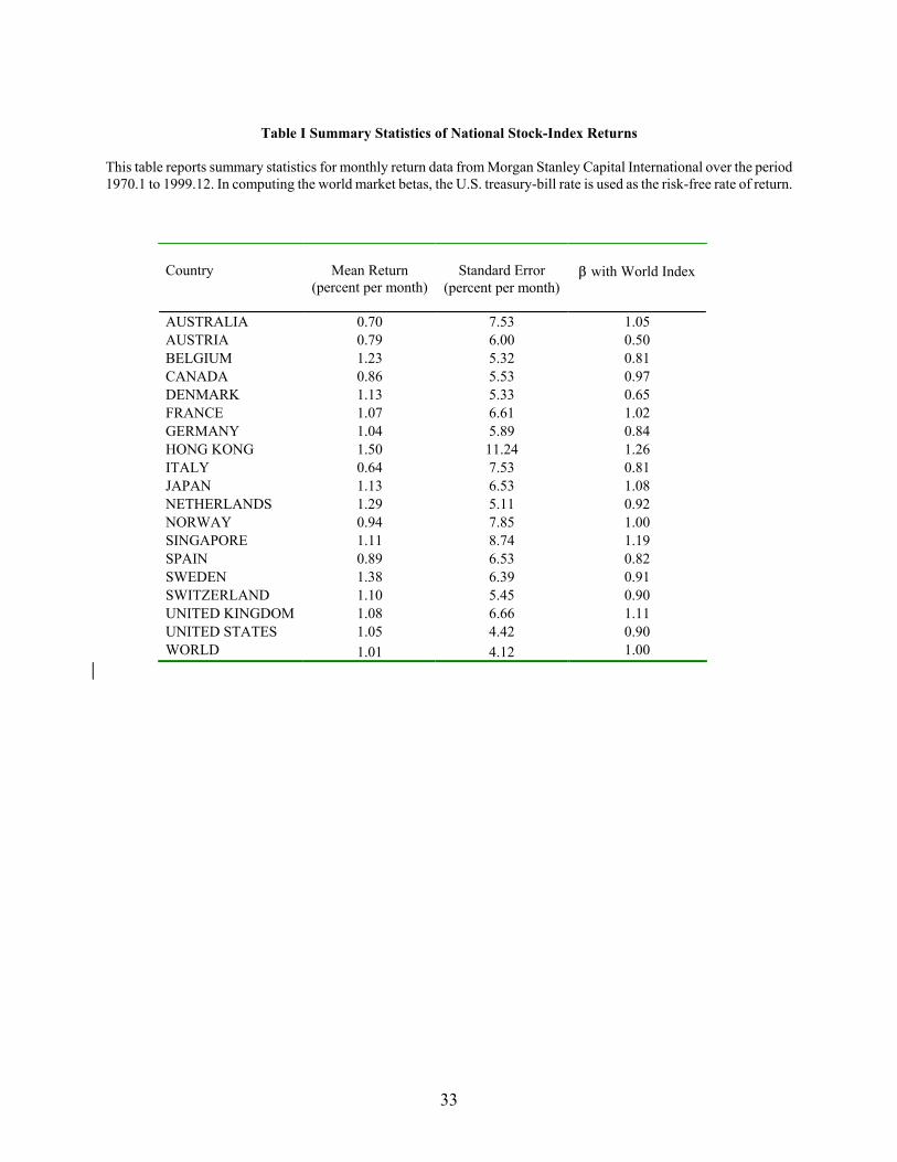
33

Table I Summary Statistics of National Stock-Index Returns

This table reports summary statistics for monthly return data from Morgan Stanley Capital International over the period 1970.1 to 1999.12. In computing the world market betas, the U.S. treasury-bill rate is used as the risk-free rate of return.

Country

Mean Return (percent per month)

Standard Error (percent per month)

β with World Index

AUSTRALIA 0.70 7.53

1.05

AUSTRIA 0.79 6.00 0.50 BELGIUM 1.23 5.32 0.81 CANADA 0.86 5.53 0.97 DENMARK 1.13 5.33 0.65 FRANCE 1.07 6.61 1.02 GERMANY 1.04 5.89 0.84 HONG KONG 1.50 11.24 1.26 ITALY 0.64 7.53 0.81 JAPAN 1.13 6.53 1.08 NETHERLANDS 1.29 5.11 0.92 NORWAY 0.94 7.85 1.00 SINGAPORE 1.11 8.74 1.19 SPAIN 0.89 6.53 0.82 SWEDEN 1.38 6.39 0.91 SWITZERLAND 1.10 5.45 0.90 UNITED KINGDOM 1.08 6.66 1.11 UNITED STATES 1.05 4.42 0.90 WORLD 1.01 4.12 1.00

34

Table II Performance of Portfolio Switching Strategies: Jegadeesh and Titman (1993) Approach This table reports the mean returns (annualized) of Max1, Max1-Min1, Max3 and Max3-Min3 portfolios formed according to the Jegadeesh and Titman (1993) momentum strategy. The shaded areas (J=3,6,9,12; K=3,6,9,12) are the combinations of J (index sorting period) and K (index holding period) originally examined by Jegadeesh and Titman (1993) for U.S. stock data.

K=1 K=3 K=6 K=9 K=12 K=15 K=18 Mean

Return t-ratio Mean

Return t-ratio Mean

Return t-ratio Mean

Return t-ratio Mean

Return t-ratio Mean

Return t-ratio Mean

Return t-ratio

J=3 Max1 0.192 3.316 0.165 3.301 0.176 3.802 0.171 3.873 0.158 3.589 0.142 3.470 0.133 3.376

Max1-Min1 -0.004 -0.056 0.038 0.650 0.070 1.418 0.080 1.903 0.065 1.670 0.023 0.663 0.005 0.171 Max3 0.164 3.637 0.158 3.781 0.155 3.803 0.159 4.109 0.153 3.867 0.135 3.590 0.142 3.858

Max3-Min3 0.025 0.558 0.034 0.889 0.045 1.367 0.058 2.136 0.046 1.795 0.013 0.564 0.013 0.578 J=6

Max1 0.171 2.687 0.206 3.647 0.188 3.729 0.175 3.545 0.148 3.063 0.131 2.985 0.138 3.316 Max1-Min1 -0.011 -0.137 0.056 0.803 0.084 1.478 0.093 1.827 0.050 1.045 0.008 0.180 0.010 0.272

Max3 0.211 4.528 0.216 4.844 0.195 4.629 0.177 4.159 0.156 3.749 0.147 3.732 0.146 3.883 Max3-Min3 0.116 2.290 0.103 2.363 0.106 2.864 0.090 2.573 0.050 1.543 0.026 0.870 0.023 0.865

J=9 Max1 0.141 2.228 0.180 3.110 0.161 2.879 0.138 2.577 0.125 2.549 0.124 2.739 0.129 3.031

Max1-Min1 0.033 0.418 0.101 1.449 0.112 1.763 0.078 1.333 0.035 0.656 0.013 0.273 0.016 0.366 Max3 0.198 3.901 0.189 3.990 0.173 3.801 0.158 3.592 0.146 3.504 0.141 3.606 0.145 3.881

Max3-Min3 0.108 2.126 0.118 2.594 0.113 2.675 0.082 2.081 0.046 1.292 0.032 0.991 0.028 0.971 J=12 Max1 0.184 2.583 0.180 2.838 0.140 2.384 0.135 2.547 0.131 2.625 0.131 2.799 0.141 3.133

Max1-Min1 0.095 1.107 0.092 1.234 0.049 0.753 0.041 0.714 0.020 0.382 0.000 0.002 0.007 0.167 Max3 0.177 3.374 0.184 3.706 0.163 3.536 0.146 3.339 0.139 3.394 0.138 3.539 0.139 3.735

Max3-Min3 0.112 2.110 0.112 2.266 0.082 1.857 0.055 1.365 0.028 0.758 0.017 0.529 0.013 0.443 J=15 Max1 0.113 1.636 0.112 1.824 0.159 2.892 0.152 2.900 0.140 2.799 0.136 2.845 0.135 2.960

Max1-Min1 -0.016 -0.199 -0.009 -0.118 0.042 0.668 0.032 0.565 0.017 0.321 -0.004 -0.075 -0.007 -0.149 Max3 0.149 2.807 0.159 3.380 0.144 3.231 0.137 3.280 0.136 3.377 0.137 3.570 0.141 3.840

Max3-Min3 0.052 0.966 0.051 1.056 0.043 0.998 0.030 0.769 0.016 0.440 0.009 0.292 0.010 0.330 J=18 Max1 0.122 1.718 0.168 2.847 0.164 2.955 0.154 2.826 0.142 2.737 0.140 2.841 0.136 2.877

Max1-Min1 -0.027 -0.341 0.056 0.825 0.044 0.712 0.040 0.670 0.008 0.142 0.001 0.013 -0.010 -0.202 Max3 0.140 2.650 0.150 3.356 0.141 3.377 0.135 3.354 0.133 3.396 0.134 3.585 0.135 3.767

Max3-Min3 0.030 0.573 0.037 0.827 0.033 0.816 0.018 0.467 0.005 0.129 0.001 0.023 -0.002 -0.054

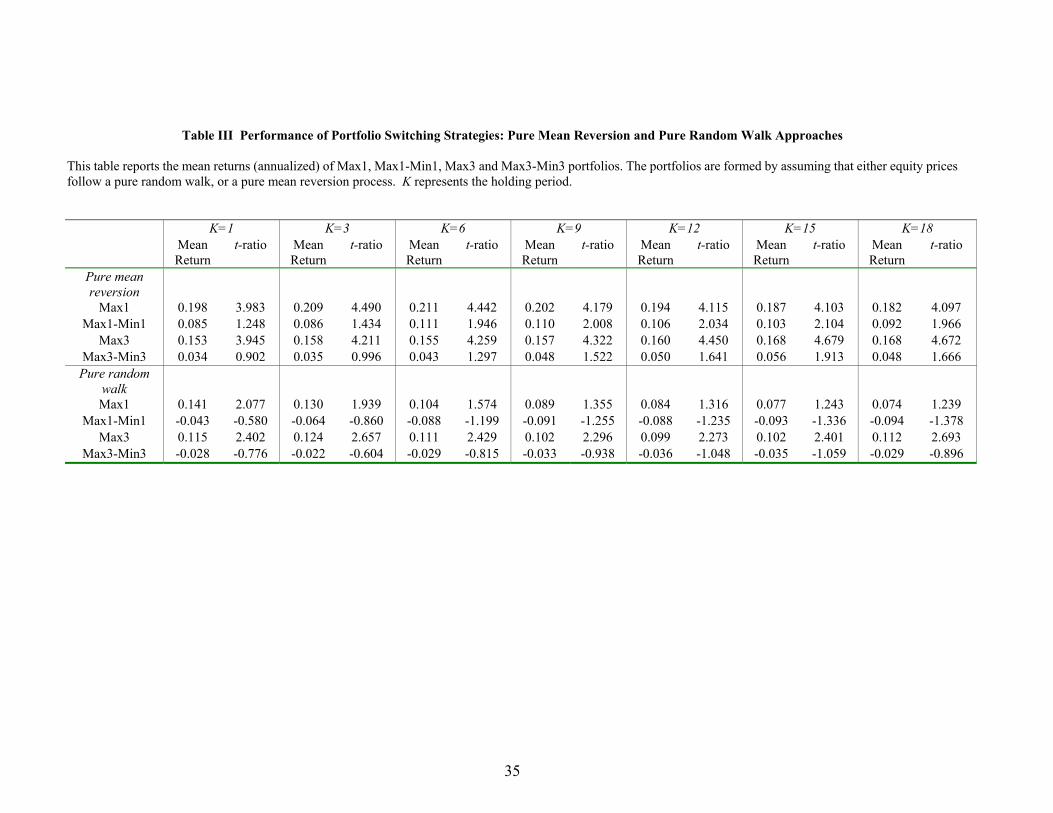
35

Table III Performance of Portfolio Switching Strategies: Pure Mean Reversion and Pure Random Walk Approaches This table reports the mean returns (annualized) of Max1, Max1-Min1, Max3 and Max3-Min3 portfolios. The portfolios are formed by assuming that either equity prices follow a pure random walk, or a pure mean reversion process. K represents the holding period.

K=1 K=3 K=6 K=9 K=12 K=15 K=18 Mean

Return t-ratio Mean

Return t-ratio Mean

Return t-ratio Mean

Return t-ratio Mean

Return t-ratio Mean

Return t-ratio Mean

Return t-ratio

Pure mean reversion

Max1 0.198 3.983 0.209 4.490 0.211 4.442 0.202 4.179 0.194 4.115 0.187 4.103 0.182 4.097 Max1-Min1 0.085 1.248 0.086 1.434 0.111 1.946 0.110 2.008 0.106 2.034 0.103 2.104 0.092 1.966

Max3 0.153 3.945 0.158 4.211 0.155 4.259 0.157 4.322 0.160 4.450 0.168 4.679 0.168 4.672 Max3-Min3 0.034 0.902 0.035 0.996 0.043 1.297 0.048 1.522 0.050 1.641 0.056 1.913 0.048 1.666 Pure random

walk

Max1 0.141 2.077 0.130 1.939 0.104 1.574 0.089 1.355 0.084 1.316 0.077 1.243 0.074 1.239 Max1-Min1 -0.043 -0.580 -0.064 -0.860 -0.088 -1.199 -0.091 -1.255 -0.088 -1.235 -0.093 -1.336 -0.094 -1.378

Max3 0.115 2.402 0.124 2.657 0.111 2.429 0.102 2.296 0.099 2.273 0.102 2.401 0.112 2.693 Max3-Min3 -0.028 -0.776 -0.022 -0.604 -0.029 -0.815 -0.033 -0.938 -0.036 -1.048 -0.035 -1.059 -0.029 -0.896

36

Table IV Performance of Portfolio Switching Strategies: Momentum with Mean Reversion This table reports the mean returns (annualized) of Max1, Max1-Min1, Max3 and Max3-Min3 portfolios. The portfolios are formed by assuming that equity prices have both momentum and mean reversion effects. For the Max-Min cases shaded numbers signify that the current strategy beats the Jagadeesh-Titman pure momentum strategy. J represents sorting period and K represents holding period.

K=1 K=3 K=6 K=9 K=12 K=15 K=18 Mean

Return t-ratio Mean

Return t-ratio Mean

Return t-ratio Mean

Return t-ratio Mean

Return t-ratio Mean

Return t-ratio Mean

Return t-ratio

J=3 Max1 0.233 4.637 0.201 4.239 0.190 3.892 0.183 3.982 0.179 3.987 0.171 3.867 0.167 3.849

Max1-Min1 0.094 1.464 0.074 1.305 0.103 1.917 0.109 2.202 0.117 2.493 0.098 2.211 0.088 2.024 Max3 0.187 4.662 0.181 4.697 0.179 4.636 0.180 4.735 0.185 4.754 0.175 4.528 0.170 4.474

Max3-Min3 0.079 2.165 0.066 1.993 0.080 2.497 0.090 2.885 0.087 2.797 0.070 2.361 0.058 2.016 J=6

Max1 0.162 2.868 0.185 3.347 0.169 3.319 0.170 3.431 0.161 3.341 0.153 3.242 0.153 3.367 Max1-Min1 0.061 0.945 0.079 1.310 0.095 1.743 0.108 2.130 0.096 1.996 0.084 1.790 0.074 1.681

Max3 0.176 4.366 0.177 4.405 0.180 4.510 0.186 4.622 0.175 4.383 0.170 4.310 0.170 4.403 Max3-Min3 0.062 1.726 0.067 1.927 0.094 2.730 0.097 2.847 0.075 2.284 0.061 1.950 0.056 1.875

J=9 Max1 0.179 3.244 0.165 3.203 0.161 3.200 0.152 3.092 0.139 2.877 0.125 2.725 0.129 2.899

Max1-Min1 0.168 2.562 0.143 2.363 0.146 2.660 0.124 2.367 0.089 1.747 0.068 1.403 0.051 1.083 Max3 0.195 4.671 0.201 4.854 0.201 4.792 0.183 4.429 0.170 4.219 0.163 4.158 0.164 4.344

Max3-Min3 0.101 2.707 0.113 3.021 0.121 3.325 0.092 2.639 0.067 2.026 0.054 1.676 0.049 1.605 J=12 Max1 0.180 3.401 0.177 3.450 0.159 3.187 0.153 3.091 0.143 3.095 0.128 2.859 0.134 3.108

Max1-Min1 0.167 2.449 0.156 2.540 0.130 2.278 0.106 1.890 0.093 1.789 0.066 1.310 0.062 1.256 Max3 0.203 4.528 0.216 4.958 0.190 4.545 0.173 4.240 0.163 4.072 0.155 4.033 0.161 4.313

Max3-Min3 0.119 2.964 0.121 3.152 0.102 2.797 0.079 2.288 0.063 1.906 0.048 1.478 0.047 1.530 J=15 Max1 0.166 3.197 0.164 3.206 0.150 2.949 0.148 3.001 0.146 3.064 0.136 2.911 0.157 3.417

Max1-Min1 0.083 1.423 0.074 1.362 0.087 1.620 0.093 1.856 0.094 1.952 0.077 1.640 0.100 2.179 Max3 0.217 5.359 0.203 5.255 0.183 4.741 0.174 4.553 0.166 4.433 0.162 4.382 0.168 4.666

Max3-Min3 0.111 3.070 0.082 2.449 0.069 2.045 0.064 1.951 0.052 1.610 0.047 1.510 0.051 1.708 J=18 Max1 0.157 2.970 0.159 3.065 0.154 3.125 0.154 3.218 0.151 3.215 0.154 3.355 0.154 3.430

Max1-Min1 0.052 0.876 0.074 1.297 0.081 1.519 0.083 1.617 0.080 1.656 0.086 1.829 0.087 1.872 Max3 0.184 4.602 0.186 4.845 0.178 4.705 0.173 4.629 0.170 4.551 0.172 4.740 0.174 4.835

Max3-Min3 0.061 1.784 0.062 1.891 0.064 2.058 0.062 2.007 0.059 1.939 0.064 2.151 0.063 2.135

37

Table V Model Parameters and Variance Decomposition

This table reports key parameter estimates of the baseline model and the implied variance decomposition. All notation follows that in the text. ),( tt MRVMOMCorr is the correlation coefficient between the mean reversion and momentum

components; and 2R is the coefficient of determination from regression equation (5).

Moment Estimate

δ 0.979

ρ 0.026

)( tRVar 3.152E-3

2ησ 3.069E-3

)( tMRVVar 7.185E-05

)( tMOMVar 5.215E-05

),( tt MRVMOMCorr -0.338

2ησ / )( tRVar (%) 97.4

)( tMRVVar / )( tRVar (%) 2.28

)( tMOMVar / )( tRVar (%) 1.66

2R (%) 2.62

38

Table VI Testing for Convergence

This table presents panel-based tests for convergence of an index relative to a benchmark index for 13 OECD countries (Our original sample of Table I excluding Australia, Denmark, Hong Kong, Singapore, and Switzerland, for which a sample of sufficient length for Industrial Production is not available). Panel A. Convergence of Relative Equity Price Indexes (1970-1999) The model is specified as: 1 1 1( )i b i b ii

t t t t tr - r = - p - p λ εα+ + ++ where p is the logarithm of a price index, r is the return rate, and i = 1,..., 12. The superscript “b” denotes a benchmark index. The benchmarks are the U.S, Japan and Germany, respectively. The null hypothesis is that equity indexes do not converge to the benchmark index, or H0: λ = 0. The alternative hypothesis is that equity indexes converge to the benchmark index with the speed of λ per month, or H1: λ > 0. The test statistics are defined as: λλ

ˆTz = and

)ˆ(ˆ λλλ /s = t , where T is the time periods in the sample, and )ˆ(λs is the standard error of λ̂ . The p-values are computed from 5,000 Monte-Carlo replications.

Relative to US Relative to Japan Relative to UK Point Estimate of λ 0.017 0.016 0.018

zλ 6.116 5.672 6.411 p-value 0.004 0.013 0.004

tλ 6.970 7.550 6.364 p-value 0.001 0.000 0.011

Panel B. Convergence of Relative Per Capita Industrial Production (1961-1999) The model is specified as: 1 1 1( )i b i b ii

t t t t tIP - IP = - IP - IP λ εα+ + +∆ ∆ + where IP is the logarithm of an industrial production index, IP∆ is the percentage change in industrial production, and i = 1,..., 12. The superscript “b” denotes a benchmark index. The benchmarks are the U.S, Japan and Germany, respectively. The null hypothesis is that industrial production indexes do not converge to the benchmark index, or H0: λ = 0. The alternative hypothesis is that industrial production indexes converge to the benchmark index with the speed of λ per month, or H1: λ > 0. The test statistics are defined as: λλ

ˆTz = and )ˆ(ˆ λλλ /s = t , where T is the time periods in the

sample, and )ˆ(λs is the standard error of λ̂ . The p-values are computed from 5,000 Monte-Carlo replications.

Relative to US Relative to Japan Relative to U.K. Point Estimate of λ 0.015 0.011 0.019

zλ 7.163 5.010 8.842 p-value 0.001 0.047 0.000

tλ 7.541 8.249 9.070 p-value 0.000 0.000 0.000

39

Table VII Comparison of Model Performance Panel A. 1. Baseline model where the mean reversion parameter is identical across countries, and the momentum parameter is identical across lags and countries; 2. Jegadeesh-Titman pure momentum; 3. Pure mean reversion; 4. Pure random walk; 5. Baseline model with forecast starting at ¼ of sample; 6. Baseline model with forecast starting at ½ of sample; and 7. Baseline model with portfolio formed one month after ranking.

Model Portfolio Mean Return t-ratio β with World Portfolio

Expected Return

Average Portfolio Turnover Rate

1 Max1 0.180 3.401 0.962 0.318 0.13 Max1-Min1 0.167 2.449 -0.301 0.393 0.16 Max3 0.203 4.528 0.984 0.260 0.10 Max3-Min3 0.119 2.964 -0.064 0.367 0.10

2 Max1 0.184 2.583 1.284 0.212 0.35 Max1-Min1 0.095 1.107 0.373 0.151 0.39 Max3 0.177 3.374 0.154 0.191 0.25 Max3-Min3 0.112 2.110 0.297 0.130 0.26

3 Max1 0.198 3.983 0.615 0.241 0.11 Max1-Min1 0.085 1.248 -0.621 0.218 0.11 Max3 0.153 3.945 0.837 0.212 0.10 Max3-Min3 0.034 0.902 -0.245 0.198 0.09

4 Max1 0.141 2.077 1.284 0.238 0.03 Max1-Min1 -0.043 -0.580 0.434 0.154 0.04 Max3 0.115 2.402 1.177 0.216 0.05 Max3-Min3 -0.028 -0.776 0.240 0.115 0.03

5 Max1 0.212 4.164 0.934 0.318 0.14 Max1-Min1 0.191 2.990 -0.292 0.389 0.17 Max3 0.215 5.180 0.970 0.262 0.09 Max3-Min3 0.132 3.448 -0.060 0.228 0.10

6 Max1 0.206 3.144 1.159 0.304 0.16 Max1-Min1 0.130 1.704 -0.047 0.361 0.17 Max3 0.230 4.183 1.069 0.260 0.11 Max3-Min3 0.081 1.760 0.052 0.278 0.10

7 Max1 0.163 3.101 0.952 0.318 0.13 Max1-Min1 0.151 2.257 -0.259 0.393 0.16 Max3 0.218 4.820 0.983 0.260 0.10 Max3-Min3 0.133 3.250 -0.074 0.296 0.10

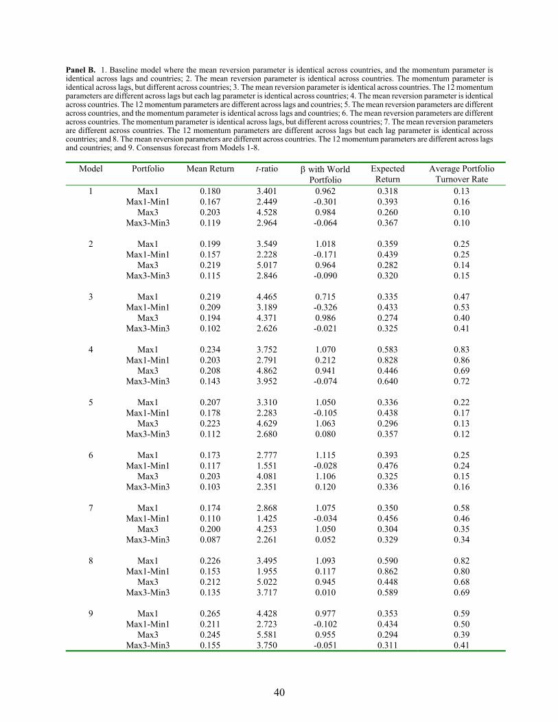
40

Panel B. 1. Baseline model where the mean reversion parameter is identical across countries, and the momentum parameter is identical across lags and countries; 2. The mean reversion parameter is identical across countries. The momentum parameter is identical across lags, but different across countries; 3. The mean reversion parameter is identical across countries. The 12 momentum parameters are different across lags but each lag parameter is identical across countries; 4. The mean reversion parameter is identical across countries. The 12 momentum parameters are different across lags and countries; 5. The mean reversion parameters are different across countries, and the momentum parameter is identical across lags and countries; 6. The mean reversion parameters are different across countries. The momentum parameter is identical across lags, but different across countries; 7. The mean reversion parameters are different across countries. The 12 momentum parameters are different across lags but each lag parameter is identical across countries; and 8. The mean reversion parameters are different across countries. The 12 momentum parameters are different across lags and countries; and 9. Consensus forecast from Models 1-8.

Model Portfolio Mean Return t-ratio β with World Portfolio

Expected Return

Average Portfolio Turnover Rate

1 Max1 0.180 3.401 0.962 0.318 0.13 Max1-Min1 0.167 2.449 -0.301 0.393 0.16 Max3 0.203 4.528 0.984 0.260 0.10 Max3-Min3 0.119 2.964 -0.064 0.367 0.10

2 Max1 0.199 3.549 1.018 0.359 0.25 Max1-Min1 0.157 2.228 -0.171 0.439 0.25 Max3 0.219 5.017 0.964 0.282 0.14 Max3-Min3 0.115 2.846 -0.090 0.320 0.15

3 Max1 0.219 4.465 0.715 0.335 0.47 Max1-Min1 0.209 3.189 -0.326 0.433 0.53 Max3 0.194 4.371 0.986 0.274 0.40 Max3-Min3 0.102 2.626 -0.021 0.325 0.41

4 Max1 0.234 3.752 1.070 0.583 0.83 Max1-Min1 0.203 2.791 0.212 0.828 0.86 Max3 0.208 4.862 0.941 0.446 0.69 Max3-Min3 0.143 3.952 -0.074 0.640 0.72

5 Max1 0.207 3.310 1.050 0.336 0.22 Max1-Min1 0.178 2.283 -0.105 0.438 0.17 Max3 0.223 4.629 1.063 0.296 0.13 Max3-Min3 0.112 2.680 0.080 0.357 0.12

6 Max1 0.173 2.777 1.115 0.393 0.25 Max1-Min1 0.117 1.551 -0.028 0.476 0.24 Max3 0.203 4.081 1.106 0.325 0.15 Max3-Min3 0.103 2.351 0.120 0.336 0.16

7 Max1 0.174 2.868 1.075 0.350 0.58 Max1-Min1 0.110 1.425 -0.034 0.456 0.46 Max3 0.200 4.253 1.050 0.304 0.35 Max3-Min3 0.087 2.261 0.052 0.329 0.34

8 Max1 0.226 3.495 1.093 0.590 0.82 Max1-Min1 0.153 1.955 0.117 0.862 0.80 Max3 0.212 5.022 0.945 0.448 0.68 Max3-Min3 0.135 3.717 0.010 0.589 0.69

9 Max1 0.265 4.428 0.977 0.353 0.59 Max1-Min1 0.211 2.723 -0.102 0.434 0.50 Max3 0.245 5.581 0.955 0.294 0.39 Max3-Min3 0.155 3.750 -0.051 0.311 0.41

41

Table VIII Percentage Overlap in the Max3 and Min3 Portfolios across Models

The models are: 1. Baseline model; 2. Jegadeesh-Titman pure momentum; 3. Pure mean reversion; 4. Pure random walk; 5. Perfect foresight; 6. The mean reversion parameter is identical across countries. The momentum parameter is identical across lags, but is different across countries; 7. The mean reversion parameter is identical across countries. The 12 momentum parameters are different across lags but identical across countries; 8. The mean reversion parameter is identical across countries. The 12 momentum parameters are different across lags and countries; 9. The mean reversion parameters are different across countries, and the momentum parameter is identical across lags and countries; 10. The mean reversion parameters are different across countries. The momentum parameter is identical across lags, but different across countries; 11. The mean reversion parameters are different across countries. The 12 momentum parameters are different across lags but identical across countries; and 12. The mean reversion parameters are different across countries. The 12 momentum parameters are different across lags and countries.

Panel A: Percentage Overlap in the Max3 Portfolio

Model 1 2 3 4 5 7 8 9 10 11 12 13 1 100 2 28 100 3 61 8 100 4 5 30 7 100 5 21 21 19 21 100 6 79 31 53 5 21 100 7 73 27 55 7 21 64 100 8 41 26 32 11 22 43 44 100 9 52 26 33 4 23 51 43 34 100

10 51 33 31 5 22 54 44 39 78 100 11 48 26 32 5 22 46 51 37 78 68 100 12 37 25 28 10 23 37 39 78 44 48 45 100

Panel B: Percentage Overlap in the Min3 Portfolio

Model 1 2 3 4 5 6 7 8 9 10 11 12 1 100 2 23 100 3 61 5 100 4 4 21 6 100 5 19 26 17 21 100 6 84 24 60 4 19 100 7 73 23 54 6 19 67 100 8 34 24 30 12 23 35 36 100 9 54 21 41 6 20 53 48 28 100

10 47 30 38 6 22 51 44 32 75 100 11 50 24 40 7 20 49 53 31 79 71 100 12 29 24 27 13 23 31 32 77 38 42 43 100

42

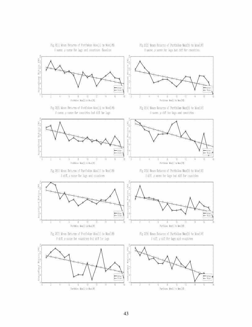
43