molecules in electric and magnetic fields

Chapter 3, page 1

3 Molecules in Electric and Magnetic Fields 3.1 Basic Equations from Electrodynamics The basis of the description of the behaviour of molecules in electric and magnetic fields are the material equations of Maxwell’s theory. The equation for the magnetic induction B is B = μ0 (H + M ) = μr μ0 H = μ0 ( 1 + χ) H . (3.01) μ0 = 4π × 10−7 V s A−1m−1 (H m−1) μ0 is the permeability of vacuum, μr is the relative permeability, which is normally taken as a scalar to describe the isotropic properties of a medium. χ is the dimensionless magnetic susceptibility. Magnetization M in equ. (3.01) has the dimensions of a magnetic field strength, and adds to the magnetic field strength H. In some textbooks you may find the magnetic polarisation J defined in analogy to electric polarisation P. It is used in B = μ0H + J, where J has the same dimension as B. For the dielectric displacement D and the induced electric polarisation P we have D = ε0 E + P = εr ε0 E = ε0 (1+ χe ) E and P = χe ε0 E = (εr − 1)ε0 E. (3.02) ε0 = 1/μ0c0

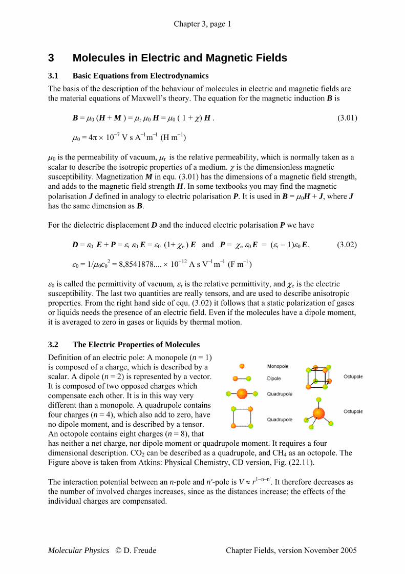
2 = 8,8541878.... × 10−12 A s V−1m−1 (F m−1) ε0 is called the permittivity of vacuum, εr is the relative permittivity, and χe is the electric susceptibility. The last two quantities are really tensors, and are used to describe anisotropic properties. From the right hand side of equ. (3.02) it follows that a static polarization of gases or liquids needs the presence of an electric field. Even if the molecules have a dipole moment, it is averaged to zero in gases or liquids by thermal motion. 3.2 The Electric Properties of Molecules Definition of an electric pole: A monopole (n = 1) is composed of a charge, which is described by a scalar. A dipole (n = 2) is represented by a vector. It is composed of two opposed charges which compensate each other. It is in this way very different than a monopole. A quadrupole contains four charges (n = 4), which also add to zero, have no dipole moment, and is described by a tensor. An octopole contains eight charges (n = 8), that has neither a net charge, nor dipole moment or quadrupole moment. It requires a four dimensional description. CO2 can be described as a quadrupole, and CH4 as an octopole. The Figure above is taken from Atkins: Physical Chemistry, CD version, Fig. (22.11). The interaction potential between an n-pole and n'-pole is V ≈ r1−n−n'. It therefore decreases as the number of involved charges increases, since as the distances increase; the effects of the individual charges are compensated.

Molecular Physics © D. Freude Chapter Fields, version November 2005

Chapter 3, page 2

Multipole expansion of N charges qn with qnn

N

=∑ =

10

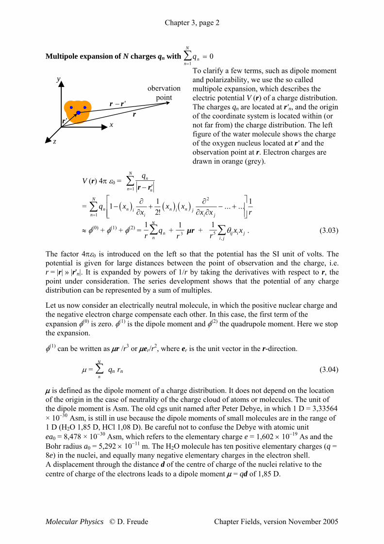
To clarify a few terms, such as dipole moment and polarizability, we use the so called multipole expansion, which describes the electric potential V (r) of a charge distribution. The charges qn are located at r'n, and the origin of the coordinate system is located within (or not far from) the charge distribution. The left figure of the water molecule shows the charge of the oxygen nucleus located at r' and the observation point at r. Electron charges are drawn in orange (grey).

y

x

z

r − r' r

r'

obervationpoint

V (r) 4π ε0 = qn

nn

N

r r− ′=∑

1

= ( ) ( ) ( )q xx

x xx x rn

n

N

n ii

n i n ji j=

∑ − + − +⎡

⎣⎢⎢

⎤

⎦⎥⎥1

2

1 12

1∂∂

∂∂ ∂!

... ...

≈ φ(0) + φ(1) + φ(2) = 1r

qnn

N

∑ + 1

3r µr +

15r

x xij i ji j

θ,

∑ . (3.03)

The factor 4πε0 is introduced on the left so that the potential has the SI unit of volts. The potential is given for large distances between the point of observation and the charge, i.e. r = |r| » |r'n|. It is expanded by powers of 1/r by taking the derivatives with respect to r, the point under consideration. The series development shows that the potential of any charge distribution can be represented by a sum of multiples.

Let us now consider an electrically neutral molecule, in which the positive nuclear charge and the negative electron charge compensate each other. In this case, the first term of the expansion φ(0) is zero. φ(1) is the dipole moment and φ(2) the quadrupole moment. Here we stop the expansion.

φ(1) can be written as μr /r3 or μer/r2, where er is the unit vector in the r-direction.

μ = qn rn (3.04) n

N

∑

μ is defined as the dipole moment of a charge distribution. It does not depend on the location of the origin in the case of neutrality of the charge cloud of atoms or molecules. The unit of the dipole moment is Asm. The old cgs unit named after Peter Debye, in which 1 D = 3,33564 × 10−30 Asm, is still in use because the dipole moments of small molecules are in the range of 1 D (H2O 1,85 D, HCl 1,08 D). Be careful not to confuse the Debye with atomic unit ea0 = 8,478 × 10−30 Asm, which refers to the elementary charge e = 1,602 × 10−19 As and the Bohr radius a0 = 5,292 × 10−11 m. The H2O molecule has ten positive elementary charges (q = 8e) in the nuclei, and equally many negative elementary charges in the electron shell. A displacement through the distance d of the centre of charge of the nuclei relative to the centre of charge of the electrons leads to a dipole moment μ = qd of 1,85 D.


Chapter 3, page 3

The vector character of µ allows the vector addition of dipole moments of different segments of a molecule. Examples are the halogen substituted benzene molecules. We use the experimentally determined dipole moment of monohalogen benzene and use that to calculate the poly-substituted benzene, under the assumption of a regular hexagon. See at left Fig. 22.2 taken from Atkins.

Now we come to the last term φ(2) in equ. (3.03), which describes the potential of a quadrupole. The quadrupole moment is

( ) ( )[ ]θ ij n n i n j n ijn

N

q x x r= −=

∑12

3 2

1

δ (3.05)

at the origin. δij is the Kronecker symbol. Although we will not discuss molecular quadrupoles and multipoles of higher order, nuclear quadrupoles play an important role in spectroscopy. From equ. (3.05) we can see that the quadrupole tensor has no trace.

Even though single magnetic charges do not exist, we can write a relationship for magnetic potential analogous to equ. (3.03). It is important that we treat the magnetic moment, which is also represented by μ, since, together with the electric dipole moment, it will be used in the electromagnetic dipole radiation in the chapter 3.5 concerning magnetic properties.

Statements about whether a molecule contains a permanent dipole moment will be done using symmetry consideration in chapter 4. E.g., cubic symmetry groups and the groups D indicate non polar molecules.

Now we consider dielectric material consisting of particles without permanent dipole moments, e.g. CO2. A moment μind can be induced through the electric polarizability α (units: Asm2/V) under the influence of an external electric field E. The corresponding polarizability tensor α is defined by

μind = α E (3.06)

This linear effect is sufficient for the consideration of weak fields. But if we are dealing with strong fields, for example in lasers, the equation

μind = α E + β E2 + γ E3 + ... (3.07)

is the basis of the consideration of effect of non-linear optics (NLO). The β term is called hyperpolarizability. Non-linear effects play an important role in the laser spectroscopy. α has the units Asm/(V/m), which is Asm2 V−1.


Chapter 3, page 4

This SI unit has not succeeded in driving out a modified cgs unit, the so-called polarizability volume α', which has the unit 10−24 cm3 = Å3 what is similar in magnitude to the molar volume. The conversion is:

04 ε

ααπ

=′ (3.08)

Some isotropic values for α'/Å3 are CCl4: 10,5; H2:0,82; H2O: 1,48; HCl: 2,63. A very anisotropic molecule is benzene with the values: isotrop: 10,3, perpendicular: 6,7, parallel: 12,8. The relationship of the size of the induced to the permanent dipole moment is clearly seen in water: It has a permanent dipole moment of 1,8 D or 6,2 × 10−30 Asm. The polarizability of water is α' = 1,48 Å3. This value has to be multiplied by 4πε0 × 10−30 ≈ 1,11 × 10−40 and becomes 1,64 × 10−40 A s m2 V−1. If we multiply that with a relatively high field strength of 107 V m−1, we get 1,64 × 10−33 Asm, which gives us an induced dipole moment more than three orders of magnitude smaller than the permanent one. Back to the induced effects: As a relationship of the induced polarisation P to the induced dipole moment μI of N particles per unit volume, the first part of the equation

EP αVN

V

N

ii == ∑

=1

1 μ , (3.09)

is valid for any particles, whereas the second equals sign is valid only for identical particles that do not influence each other. Nonpolar molecules only have displacement polarizability. In gases there is no mutual influence of the induced dipole moment μind between the particles and we have

EP αρ

MN A= (3.10)

with the Avogadro number NA, the density ρ and the mol mass M. From equ. (3.10) and equ. (3.02) we get

αερε0

Ar 1

MN

+= . (3.11)

With this and the equation below we can determine the polarizability a of the molecules, if we know the density ρ, the molar mass M, the capacitances of an empty capacitor (C0) and one filled with the gas under study (C), by means of the equation

0

r CC

=ε . (3.12)


Chapter 3, page 5

In materials of higher density, the dipoles create an additional field which affect their neighbours. This field has the same direction as the external field and depends on the geometry. Lorenz calculated for a spherical hollow space in a dielectric with the isotropic polarization P, that the field local to the hollow space Elocal is increased relative to the external field E by the extra field P/3ε0. See the figure on the left.

With that, equ. (3.10) becomes

⎟⎟⎠

⎞⎜⎜⎝

⎛+=

0

A

3εα

ρ PEM

NP (3.13)

With equ. (3.02), we can replace E:

Eexternal

+ + + +

− − − − Eadditional

( )( )( )αεεε

εεεα

ρ 132

31 r0

r

0r0A −+

=⎟⎟⎠

⎞⎜⎜⎝

⎛+

−=

PPPNPM . (3.14)

With some rearrangement, we get the Clausius-Mosotti equation

ααερε

ε ′π=≡=

+−

Am0

A

r

r

34

321 NPNM , (3.15)

which connects the macroscopic parameters εr, ρ, and M with the molecular quantity α, and also defines the molar polarizability Pm.

Our previous consideration have assumed static fields, which are caused by a direct current (DC) source applied to a capacitor If we replace DC by AC (alternating current) with the frequency ν, we get the corresponding magnetization of the field only in the case, if the charges can change their orientation quickly enough.

The electronic polarizability produced by shifting the positively charged nucleus with respect to the negative electron shell (in molecules and in spherically symmetric atoms) takes place in less than 10−14 s.

The polarisation by the shifting or vibration of the ions in a molecule or lattice (ion polarization, distortion polarization) happens a thousand times more slowly, on the order of 10−11 s. Both types of polarization are united under the term of displacement polarization.

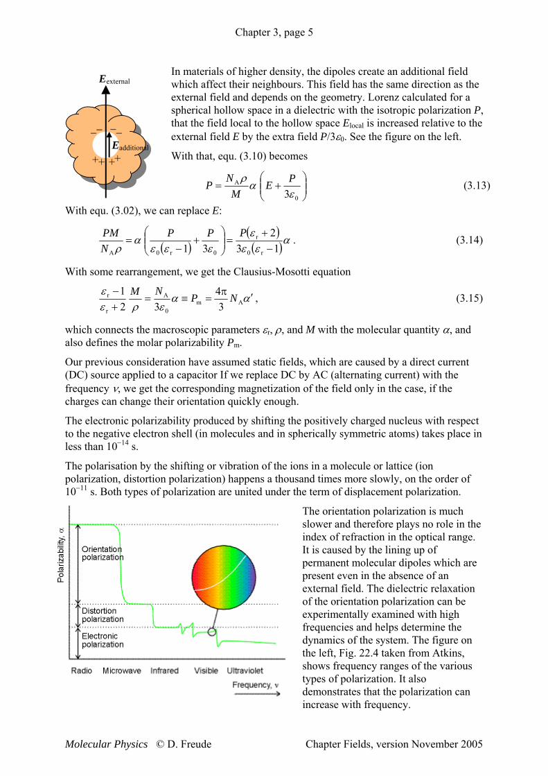
The orientation polarization is much slower and therefore plays no role in the index of refraction in the optical range. It is caused by the lining up of permanent molecular dipoles which are present even in the absence of an external field. The dielectric relaxation of the orientation polarization can be experimentally examined with high frequencies and helps determine the dynamics of the system. The figure on the left, Fig. 22.4 taken from Atkins, shows frequency ranges of the various types of polarization. It also demonstrates that the polarization can increase with frequency.


Chapter 3, page 6

In chapter 3.3 we will show that for the refractive index nr = c0/c, the Maxwell relation nr

2 = εr applies. Using that relationship, we can write the Clausius-Mossotti equation (3.15) as

m2

2

21 PM

nn

r

r =+−

ρ. (3.16)

According to our earlier assessments, as the frequency increases, optical excitement should have a lower polarization and according to equ. (3.16) a lower index of refraction as well. This should happen because the higher frequencies, the less of a role the distortion polarization plays.

Experiment, however, shows in a few cases exactly the opposite relationship, as shown to the left in table 22.2 taken from Atkins. This dispersion (increasing polarization or increasing index of refraction with increasing frequency) is due to the frequency of the incoming light being close to the resonance frequency of the system. This will be more deeply discussed in chapter 3.3.

We now return to polar molecules. Although the displacement polarization of dielectric substances is hardly dependent on the temperature, the orientation polarization of polar molecules in paraelectric substances has a strong temperature dependence. The calculation of the temperature dependency of the polarization was first calculated by Paul Langevin in 1900 in the following way: A molecule at an angle θ to the applied external electric field E, and with a permanent dipole moment µ, contributes μ cosθ to the macroscopic dipole moment and −μ E = −μ E cosθ to the total energy (Energy = −μ E). Using Boltzmann statistics, we get the probability PBoltzmann that the molecule will have the angle θ:

( )( ) kT

Exx

xP μ

θθθ

θ==

∫π mit

dsincosexp

cosexp

0

Boltzmann . (3.17)

The integral in the denominator normalizes the probability to one over all possible orienta-tions. The average dipole moment in the direction of the field is determined using equ. (3.17)

( )

( )∫∫

∫ π

π

π==

0

0

0 Boltzmanndsincosexp

dsincoscosexpdsincos

θθθ

θθθθμθθθμμ

x

xP . (3.18)


Chapter 3, page 7

By substituting y = cosθ and dy = − sinθ dθ, we get

( )

( )∫∫

1

−

1

−=

1

1

dexp1

dexp

yxy

yxyyμμ . (3.19)

From integral tables, we use

x

yxx

yyxx

xyxxxx

xy−1

−

−−1

−

−=

−−

+= ∫∫

eedeundeeeede121

. (3.20)

From equ. (3.19) and equ. (3.20) we get

kT

Exx

xx

LL xx

xx μμμ =−=−−+

== −

−

und1coth1eeeemit , (3.21)

where L is the Langevin function. If we use the dipole moment of water, which is 6,2 × 10−30 Asm, and the relatively large field strength of 107 V m−1, we get 6,2 × 10−23 VAs, which is comparable to kT = 4,14 × 10−21 VAs at room temperature. Parameter x in equ. (3.21) is a very small number. Terms past the linear term (second term) can be neglected in the series expansion of the coth x in equ. (3.21). The Langevin function can be replaced by L ≈ x/3 = μE/3kT (high temperature approximation). It follows that

kT

E3

2μμ = , (3.22)

and with the particle number per volume NAρ/M, the orientation polarization is

kT

EM

NP

3

2A

nOrientatioμρ

= . (3.23)

An similar equation was first developed as a Curie law for temperature dependent paramagnetism.

Applied to paraelectric substances, we can write

⎟⎟⎠

⎞⎜⎜⎝

⎛++=⎟⎟

⎠

⎞⎜⎜⎝

⎛+=+ kTM

NE

kTMN

P r 31and

3

2

0

A2

AntDisplacemenOrientatio

μαε

ρεμα

ρ (3.24)

for the sum of dielectric and paraelectric polarisation instead of equ. (3.10).

The same overlapping of both effects changes the Clausius-Mosotti equation, equ. (3.15), to

m

2

0

A

r

r

3321 P

kTNM

≡⎟⎟⎠

⎞⎜⎜⎝

⎛+=

+− μα

ερεε . (3.25)

Equation (3.25) is known as the Debye equation. If we measure the temperature dependency of the relative dielectric constant, and write down the molar polarisation against 1/T, we get μ as the slope according to equ. (3.25), and α as the y-intersect. For gases, 1 − εr is in the magnitude 10−3, for water at 300 K is εr = 78,5.


Chapter 3, page 8

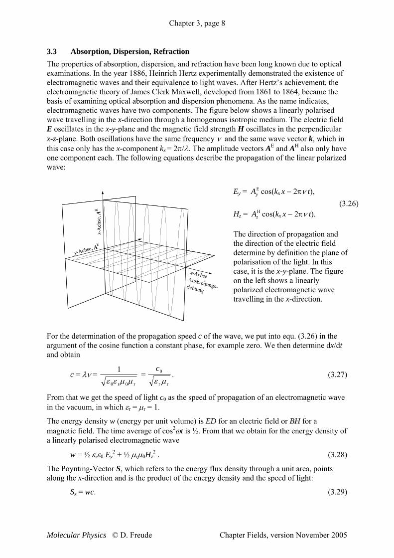
3.3 Absorption, Dispersion, Refraction The properties of absorption, dispersion, and refraction have been long known due to optical examinations. In the year 1886, Heinrich Hertz experimentally demonstrated the existence of electromagnetic waves and their equivalence to light waves. After Hertz’s achievement, the electromagnetic theory of James Clerk Maxwell, developed from 1861 to 1864, became the basis of examining optical absorption and dispersion phenomena. As the name indicates, electromagnetic waves have two components. The figure below shows a linearly polarised wave travelling in the x-direction through a homogenous isotropic medium. The electric field E oscillates in the x-y-plane and the magnetic field strength H oscillates in the perpendicular x-z-plane. Both oscillations have the same frequency ν and the same wave vector k, which in this case only has the x-component kx = 2π/λ. The amplitude vectors AE and AH also only have one component each. The following equations describe the propagation of the linear polarized wave:

z-A

chse

, AH

y-Achse, AE

x-AchseAusbreitungs-richtung

Ey = cos(kx AyE x − 2πν t),

(3.26) Hz = cos(kx Az

H x − 2πν t). The direction of propagation and the direction of the electric field determine by definition the plane of polarisation of the light. In this case, it is the x-y-plane. The figure on the left shows a linearly polarized electromagnetic wave travelling in the x-direction.

For the determination of the propagation speed c of the wave, we put into equ. (3.26) in the argument of the cosine function a constant phase, for example zero. We then determine dx/dt and obtain

c = λν = 1

0 0ε ε μ μr r

= c0

ε μr r

. (3.27)

From that we get the speed of light c0 as the speed of propagation of an electromagnetic wave in the vacuum, in which εr = μr = 1.

The energy density w (energy per unit volume) is ED for an electric field or BH for a magnetic field. The time average of cos2ωt is ½. From that we obtain for the energy density of a linearly polarised electromagnetic wave

w = ½ εrε0 Ey2 + ½ μrμ0Hz

2 . (3.28)

The Poynting-Vector S, which refers to the energy flux density through a unit area, points along the x-direction and is the product of the energy density and the speed of light:

Sx = wc. (3.29)


Chapter 3, page 9

From that we arrive at the important conclusion, that the energy flux of the radiation in the direction of propagation depends on the squares of the amplitudes of the field strengths.

The figure on the left shows the energy flux of an electromagnetic wave, propagating in the x-direction. The wave vector k and the Poynting vector S also point in the x-direction. It takes the energy enclosed in the box the time Δt to flow through the surface A. If we set Δt to one second and set A equal to the unit area, we get for the energy density a power density of the same numerical value.

cΔt

A

x, k, S

The phase speed c = λν, which is defined as the product of wavelength and frequency, is reduced in comparison to speed of light in a vacuum, c0, when the electromagnetic wave travels through a medium with an index of refraction n > 1. The reduced value is c = c0 /n. We will show that the frequency dependency of n leads to a dispersion, which can be described using a classical model. It will be also shown that the imaginary part of a complex index of refraction describes the damping of an electromagnetic wave.

For this presentation we consider an electric field with the amplitude vector AE = (0, E0, 0), which has a complex time dependency exp(iωt) instead of the cos ωt of equ. (3.26). The differential equation of a damped oscillation forced by an external field is

m dd

2 yt 2 + mγ

ddyt

+ mω02 y = q E0 exp(iωt), (3.30)

where the mass of the oscillator is m, the charge q, and the characteristic frequency ω0. γ is the damping constant. With an exponential trial solution of y = y0 exp(iωt) we obtain

y0 = ( )qE

m0

02 2 iω ω γω− +

(3.31)

as the complex amplitude of the oscillation. An induced electric dipole moment μind appears in the y direction:

μy = q y = ( )q E

m

20

02 2 iω ω γω− +

exp(iωt). (3.32)

With N oscillators per unit volume, we obtain

Pind = χe ε0 E = N μ (3.33)

as the induced electric polarisation, and with that a complex susceptibility

χe = ( )q N

m

2

0 02 2ε ω ω γω i− +

. (3.35)

The real and imaginary parts of χe are not independent, as can be shown by multiplying numerator and denominator of equ. (3.35) by the conjugated complex of the parenthesis


Chapter 3, page 10

From the definition n = c0/c , μr = εr = 1for vacuum and equ. (3.27), it follows that

n = cc0 = μ εr r . (3.36)

Since we are not considering ferromagnetic materials, we can set μr = 1 with sufficient accuracy, and we obtain the Maxwell relation

n = ε r = 1+ χe . (3.37)

We should note that these quantities are frequency dependent. For example, the orientation polarization mentioned earlier has no effect on the susceptibility in the optical frequency range. From equations (3.35) and (3.37) it follows that the index of refraction represents the complex quantity

n2 = 1 + ( )q N

m

2

0 02 2ε ω ω γω i− +

. (3.38)

To separate this into real and imaginary components, different conventions are in use. We write

n = n' − i n". (3.39)

When n ≈ 1, which is the case in gaseous media, we can make the approximation n2 − 1 = (n + 1) ( n − 1) ≈ 2 (n − 1). Near the resonant frequency we find |ω − ω0| « ω0 or ω + ω0 ≈ 2ω0 ≈ 2ω. With that we have

n' = 1 + ( ) ( )

Nqm

2

0 0

0

02 24 2ε ω

ω ω

ω ω γ

−

− + / (3.40)

and

n" = ( ) ( )

Nqm

2

0 0 02 28 2ε ωγ

ω ω γ− + / . (3.41)

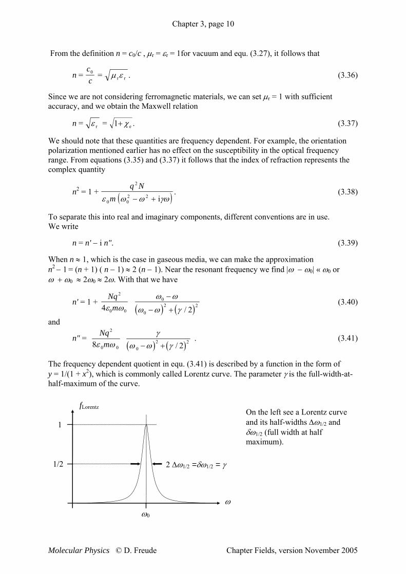
The frequency dependent quotient in equ. (3.41) is described by a function in the form of y = 1/(1 + x2), which is commonly called Lorentz curve. The parameter γ is the full-width-at-half-maximum of the curve.

2 Δω1/2 =δω1/2 = γ

ω0

fLorentz

ω

1

1/2

On the left see a Lorentz curve and its half-widths Δω1/2 and δω1/2 (full width at half maximum).


Chapter 3, page 11

The meaning of the real and imaginary components can be clarified by the following considerations: Analogous to equ. (3.26), we have for a wave propagating in the x-direction Ey = exp [i(ωt − kxAy

E x)]. (3.42) The wave vector k can be replaced by nk0, where k0 with |k0 | = ω/c0 is the wave vector in the vacuum. From equation (3.39) and (3.42) it follows that Ey = exp[i (ωt − k0x {n'−in"} x)] = exp[−n"xω/c0] exp[ik0x (c0 t − n'x)]. (3.43) Ay

E AyE

The first exponent on the right side of equ. (3.43) describes a damping of the wave. Later we will show how the absorption, described by the imaginary part of the index of refraction n", is related to experimentally measurable extinction coefficient. The second exponent describes the dispersion. In connection with equ. (3.40), we get from that the dependency of the phase speed on the frequency. 3.4 Intermolecular Interactions The electrical properties of molecules are as important for the intermolecular interactions as the absorption and dispersion. Although the repulsive forces are not entirely describable using electrostatic interactions, the van der Waals forces whose basis is the Coulomb interaction is describable. The potential energy of two point charges q1 and q2 separated by the distance r is

rqqV 21

41

0π=

ε. (3.44)

Now we will calculate the interaction of a fixed dipole μ1 = d q1 with a charge q2. Let us consider a simple model with a charge on the axis of the dipole moment, see left. For d « r and x = d/r « 1 we obtain from superimposition the attraction and repulsion of the individual charges

d r

q1 −q1 q2

22121212121

44111

441

rq

rxqq

xrqq

drqq

rqqV

0000 π−=

π−≈⎟

⎠⎞

⎜⎝⎛

++−

π=⎟

⎠⎞

⎜⎝⎛

++

−π

=ε

μεεε

. (3.45)

We broke off the series

...11

1 32 ++=±

xxxx

mm (3.46)

after the linear term. It is apparent from the diagram and equ. (3.45) that the potential is zero for a perpendicular orientation of the dipole moment and the distance vector. For all other geometries we get a potential proportional to r−2.


Chapter 3, page 12

This is changed if the dipole can freely rotate, for example around an axis perpendicular to r. We label the nuclear charges with −q1 and let the centre of the electron charges q1 freely rotate at a distance d from the fixed centre of nuclear charge. We replace the rotation by the two extreme points. One of these points is shown in the figure above. At the other point, the charge −q1 is at a distance r − d from the charge q2 on the dipole axis. We add the potentials of these two orientations (and divide the result by two to get an average potential). In doing this, we have to expand the parentheses of equ. (3.45):

⎟⎟⎠

⎞⎜⎜⎝

⎛⎥⎦⎤

⎢⎣⎡

−+−+⎥⎦

⎤⎢⎣⎡

++−⇒⎟

⎠⎞

⎜⎝⎛

++−

xxx 111

111

111 . (3.47)

In the expansion of the fractions in equ. (3.47) the terms of zero- and first-order cancel out, see equ. (3.46), and the even terms starting at the second order remain, i.e. d2/r2. If we put this back in equ. (3.45), we get a dependency of r−3. Rotations of the interaction partner raise the negative power of the distance dependency of the potential. The fact that the potential from equ. (3.45) by the rotation gets multiplied by the factor d/r « 1, indicates a reduction of the interaction potential as the negative power increases.

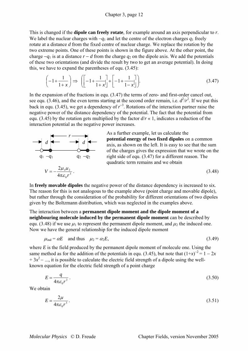
As a further example, let us calculate the potential energy of two fixed dipoles on a common axis, as shown on the left. It is easy to see that the sum of the charges gives the expression that we wrote on the right side of equ. (3.47) for a different reason. The quadratic term remains and we obtain

r

d

q1 −q1

d

q2 −q2

321

42

rV

0π−=

εμμ . (3.48)

In freely movable dipoles the negative power of the distance dependency is increased to six. The reason for this is not analogous to the example above (point charge and movable dipole), but rather through the consideration of the probability for different orientations of two dipoles given by the Boltzmann distribution, which was neglected in the examples above.

The interaction between a permanent dipole moment and the dipole moment of a neighbouring molecule induced by the permanent dipole moment can be described by equ. (3.48) if we use μ1 to represent the permanent dipole moment, and μ2 the induced one. Now we have the general relationship for the induced dipole moment

μind = αE and thus μ2 = α2E, (3.49)

where E is the field produced by the permanent dipole moment of molecule one. Using the same method as for the addition of the potentials in equ. (3.45), but note that (1+x)−2 = 1 − 2x + 3x2 − ..., it is possible to calculate the electric field strength of a dipole using the well-known equation for the electric field strength of a point charge

24 rqE

0π=

ε. (3.50)

We obtain

342

rE

0π=

εμ . (3.51)


Chapter 3, page 13

Equation (3.51) with equ. (3.49) put into equ. (3.48) gives

62

21

31

321

42

42

rrrV

000 π′

−=ππ

−=ε

αμεμ

εαμ , (3.52)

where α' is the cgs unit of the polarizability introduced in equ. (3.08). Since the induced dipole moment always has the same direction as the permanent dipole, the mobility of the molecules has no effect on V(r). The electric interaction of nonpolar molecules occurs due to fluctuations in the electron density distribution of molecules or noble gases. Let us consider a molecule 1, which has a time dependent dipole moment due to fluctuations of the electron density. Even though this dipole moment averages out in short time frames, it is always inducing a codirectional dipole moment in the neighbouring molecule 2. Due to this induced dipole moment, there is always an attractive interaction with a r−6-dependency. The strength of the interaction also depends on the polarizability of molecule 1, since this affects the creation of the fluctuating dipole moment. This dispersion interaction, first described by Fritz London, is described by the empirically discovered London formula:

2121

2162

3 αα ′′+

−=II

IIr

V . (3.53)

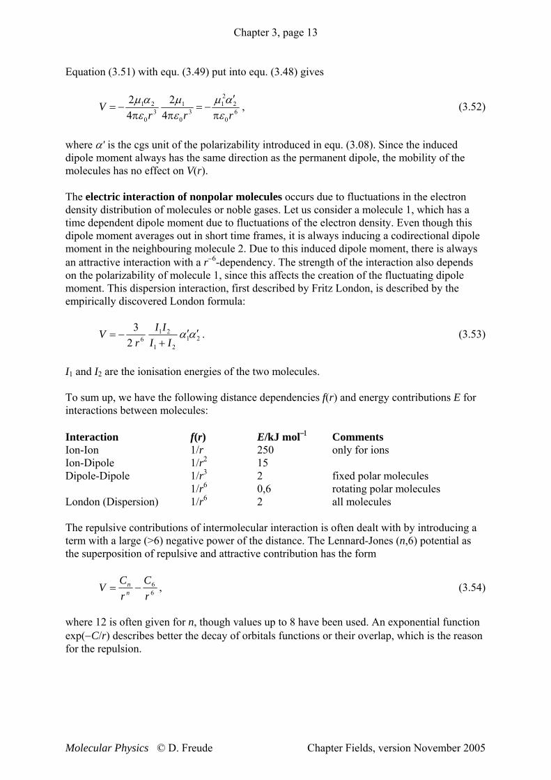
I1 and I2 are the ionisation energies of the two molecules. To sum up, we have the following distance dependencies f(r) and energy contributions E for interactions between molecules: Interaction f(r) E/kJ mol−1 Comments Ion-Ion 1/r 250 only for ions Ion-Dipole 1/r2 15 Dipole-Dipole 1/r3 2 fixed polar molecules 1/r6 0,6 rotating polar molecules London (Dispersion) 1/r6 2 all molecules The repulsive contributions of intermolecular interaction is often dealt with by introducing a term with a large (>6) negative power of the distance. The Lennard-Jones (n,6) potential as the superposition of repulsive and attractive contribution has the form

66

rC

rCV n

n −= , (3.54)

where 12 is often given for n, though values up to 8 have been used. An exponential function exp(−C/r) describes better the decay of orbitals functions or their overlap, which is the reason for the repulsion.


Chapter 3, page 14

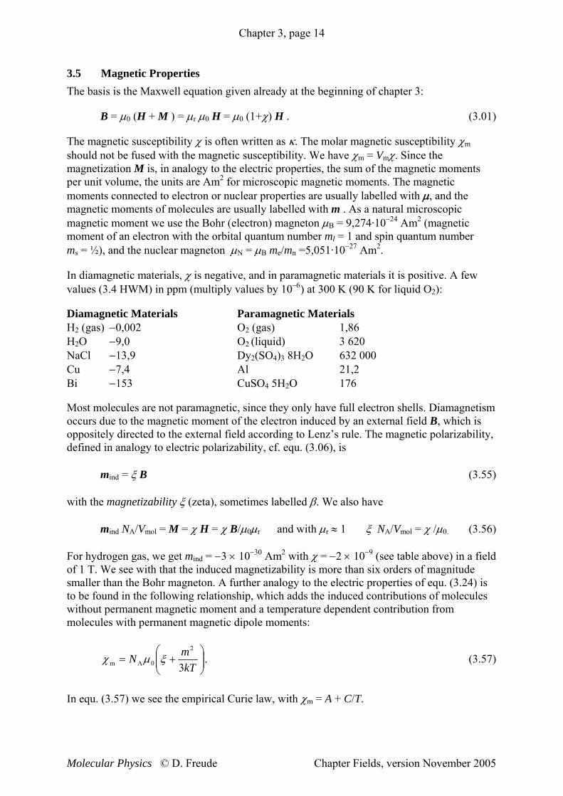
3.5 Magnetic Properties The basis is the Maxwell equation given already at the beginning of chapter 3: B = μ0 (H + M ) = μr μ0 H = μ0 (1+χ) H . (3.01) The magnetic susceptibility χ is often written as κ. The molar magnetic susceptibility χm should not be fused with the magnetic susceptibility. We have χm = Vmχ. Since the magnetization M is, in analogy to the electric properties, the sum of the magnetic moments per unit volume, the units are Am2 for microscopic magnetic moments. The magnetic moments connected to electron or nuclear properties are usually labelled with μ, and the magnetic moments of molecules are usually labelled with m . As a natural microscopic magnetic moment we use the Bohr (electron) magneton μB = 9,274·10−24 Am2 (magnetic moment of an electron with the orbital quantum number ml = 1 and spin quantum number ms = ½), and the nuclear magneton μN = μB me/mn =5,051·10−27 Am2. In diamagnetic materials, χ is negative, and in paramagnetic materials it is positive. A few values (3.4 HWM) in ppm (multiply values by 10−6) at 300 K (90 K for liquid O2): Diamagnetic Materials Paramagnetic Materials H2 (gas) −0,002 O2 (gas) 1,86 H2O −9,0 O2 (liquid) 3 620 NaCl −13,9 Dy2(SO4)3 8H2O 632 000 Cu −7,4 Al 21,2 Bi −153 CuSO4 5H2O 176 Most molecules are not paramagnetic, since they only have full electron shells. Diamagnetism occurs due to the magnetic moment of the electron induced by an external field B, which is oppositely directed to the external field according to Lenz’s rule. The magnetic polarizability, defined in analogy to electric polarizability, cf. equ. (3.06), is mind = ξ B (3.55) with the magnetizability ξ (zeta), sometimes labelled β. We also have mind NA/Vmol = M = χ H = χ B/μ0μr and with μr ≈ 1 ξ NA/Vmol = χ /μ0. (3.56) For hydrogen gas, we get mind = −3 × 10−30 Am2 with χ = −2 × 10−9 (see table above) in a field of 1 T. We see with that the induced magnetizability is more than six orders of magnitude smaller than the Bohr magneton. A further analogy to the electric properties of equ. (3.24) is to be found in the following relationship, which adds the induced contributions of molecules without permanent magnetic moment and a temperature dependent contribution from molecules with permanent magnetic dipole moments:

⎟⎟⎠

⎞⎜⎜⎝

⎛+=

kTmN3

2

0Am ξμχ . (3.57)

In equ. (3.57) we see the empirical Curie law, with χm = A + C/T.


Chapter 3, page 15

All molecules have a diamagnetic contribution to their susceptibility. This is due to the circulating currents in the ground state of the molecule’s occupied orbitals. If the circulation is forced to occur in normally unoccupied higher-energy orbitals, we get a temperature independent paramagnetism (TIP). If the molecule contains unpaired electrons, the temperature dependent spin paramagnetism dominates. This is the basis of electron spin resonance (ESR, EPR) and will be explained here in more detail. A material is called paramagnetic if it has no macroscopic magnetic moment in the absence of an external magnetic field, but has a magnetic moment in the direction of the field, if an external magnetic is applied. We can imagine that the randomly oriented microscopic magnetic dipole moments of unpaired electrons in a paramagnetic material are oriented by the application of an external field. The existence of such magnetic moments is equal to the existence of electron shells not completely closed, or the existence of unpaired electrons. Paired electrons have the same quantum numbers n, l, m, but different spin quantum numbers s = +½ and s = −½. In atoms and molecules with closed electron shells, all electrons are paired, i.e. the resulting orbital and spin moments are zero. To examine such particles with EPR, they have to be moved into a paramagnetic ground state, for example with radiation (for example, the construction of free radicals or triplet states).

Electron spin paramagnetism allows EPR spectroscopy on the following substances:

a) Free radicals in solids, liquids, or gases, which according to definition represent an atom, molecule or ion with an unpaired electron, for example CH3. Free radicals are instable. They have a finite lifetime and can be created by radiation.

b) The naturally existing ions of the transition metals, which belong to the 3d, 4d, 5d, 4f and 5f groups of the periodic table, compose more than half of the elements of the periodic table. The palette of the positively to negatively charged ions contains up to seven unpaired electrons.

To describe the orbital and spin magnetism, we will begin with a classical picture and then consider the quantum mechanical aspects: The electron in a circular orbit with radius r and angular frequency ω creates a current I = −eω/2π, where e = 1,602 × 10−19 C denotes the elementary charge. In general, the magnetic moment of a current I, which encircles the surface A, is µ = IA. With A = r2π follows µ = −½ e ω r2. Using the angular momentum L = me r2 ω and electron mass me = 9,109 × 10−31 kg, we get for the orbital magnetism a magnetic moment which depends on L:

µL = −em2 e

L . (3.58)

For spin magnetism, we start with a rotating sphere (the axis of rotation goes through the centre of mass) of mass me and charge −e. We then divide this sphere into small volume elements, in which the relationship of the segment charge through the segment mass is independent of the segment size. We then follow the same steps for each segment that we followed for the electron in a circular orbit. In the final summation, the individual contributions do not depend on the distance r of the segment of charge from the midpoint. We arrive for the dipole moment of spin magnetism at

µS = −em2 e

S , (3.59)


Chapter 3, page 16

what is analogous to equ. (3.58), but S is the spin of the electron. In quantum mechanics, it is well known that because of the quantization of the angular momentum, the absolute value is: L = +h l l( 1) and ( )S = +h s s 1 . (3.60) here l is the orbital angular momentum quantum number and s is the spin quantum number. The components in the direction of an external magnetic field in the z direction are: Lz = lz h ≡ ml h ≡ m h bzw. Sz = msh ≡ s h. (3.61) There are 2l+1 directional quantum numbers (magnetic quantum numbers) for the orbital magnetism: ml ≡ m = −l,−l +1, ..., l−1, l (3.62) and only two directional quantum numbers for electron spin magnetism ms ≡ s = −½, +½, (3.63) the use of s for the electron spin quantum number +½ and also for the directional quantum numbers ±½ could be a source of confusion. If we consider the z-component of the magnetic moment in equ. (3.58) and set the angular momentum Lz with h to the smallest value other than zero from equ. (3.61), we get as an elementary unit of the magnetic orbital moment in an external magnetic field the Bohr magneton:

µB = −em2

9 274 10 24

e

2JmVs

h = ⋅ −, . (3.64)

Based on the Bohr magneton, we introduce the g-factor (which is important in EPR) for an arbitrary magnetic quantum number m: ( )μ = g m mμB 1+ . (3.65) We will subsequently use small letters for the quantum numbers of individual electrons and capitals for the total quantum numbers of several electrons in a shell, as explained in chapter 4. By comparing equ. (3.65) to equ. (3.58) and equ. (3.60) it immediately follows that for the orbital magnetism gL = 1. This has been experimentally shown with a precision of 10−4. For spin magnetism of the free electron, we had a g-factor in equ. (3.59), (3.60), and (3.65) which is not in agreement with experimental results. Already in equ. (3.59) if we were to introduce the quantity ½h for the electron spin S with equ. (3.62) and equ. (3.63), we would have a contradiction with the experimentally proven result, that we get a whole Bohr magneton for the magnetic spin moment of the electron with the spin quantum number s = ½. In other words, it is approximately equal to the that belonging to the orbital angular momentum quantum number l = 1.


Chapter 3, page 17

Apparently the classical considerations fail for spin magnetism, although they were successful in the case of orbital magnetism. This failing of the classical model is called the magnetomechanical anomaly of the free electron. The correspondence between theory and experiment was restored by Paul Adrien Maurice Dirac in 1928 with relativistic quantum mechanics. The most accurate current value for the g-factor of the free electron is ge = 2,002319304386(20).

The magnetic resonance is based on the so-called the Zeeman resonance effect, i.e. the transitions between states which come to being through the magnetic splitting of a state, normally the ground state. For the sake of completeness, we should explain here the normal and anomalous Zeeman effect, which was found in the optical spectroscopy.

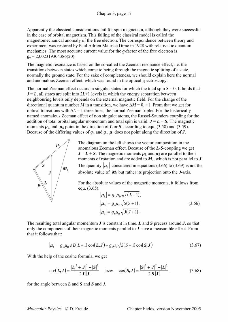
The normal Zeeman effect occurs in singulet states for which the total spin S = 0. It holds that J = L, all states are split into 2L+1 levels in which the energy separation between neighbouring levels only depends on the external magnetic field. For the change of the directional quantum number M in a transition, we have ΔM = 0, ±1. From that we get for optical transitions with ΔL = 1 three lines, the normal Zeeman triplet. For the historically named anomalous Zeeman effect of non singulet atoms, the Russel-Saunders coupling for the addition of total orbital angular momentum and total spin is valid: J = L + S. The magnetic moments µL and µS point in the direction of L or S, according to equ. (3.58) and (3.59). Because of the differing values of gL and ge, µJ does not point along the direction of J.

J

L

S

µS

µL

MJ

The diagram on the left shows the vector composition in the anomalous Zeeman effect. Because of the L-S-coupling we get J = L + S. The magnetic moments µL and µS are parallel to their moments of rotation and are added to MJ, which is not parallel to J. The quantity μ J considered in equations (3.66) to (3.69) is not the absolute value of MJ but rather its projection onto the J-axis. For the absolute values of the magnetic moments, it follows from equ. (3.65):

( )

( )

( )

μ

μ

μ

L L B

S e B

J J B

= +

=

= +

g L L

g S S

g J J

μ

μ

μ

1

1

1

,

,

.

+ (3.66)

The resulting total angular momentum J is constant in time. L and S precess around J, so that only the components of their magnetic moments parallel to J have a measurable effect. From that it follows that:

( ) ( ) ( ) ( )μJ L B e B= + + +g L L g S Sμ μ1 cos cosL,J S,J1 (3.67) With the help of the cosine formula, we get

( ) ( )cos cosL,JL J S

L JS,J

S J LS J

=+ −

=+ −2 2 2 2 2

2bzw.

2

2. (3.68)

for the angle between L and S and S and J.


Chapter 3, page 18

With L = +h L L( 1) , compare equ. (3.60) and the relevant equations for S and J,

( )( ) ( ) ( ){ }( )

( )μJ B

e L e L=+ + + + − + −

+μ

J J g g S S L L g g

J J

1 1 1

2 1. (3.69)

If we connect equ. (3.69) with the lower line in equ. (3.66) and further sets 2gL = ge = 2, we get the factor:

( ) ( ) ( )

( )gJ J S S L L

J JJ =+ + + − +

+3 1 1

2 11

, (3.70) which was named after Alfred Landé. He calculated this factor using the Bohr-Sommerfeld-quantum mechanics with the quantum numbers J 2 instead of J(J+1) etc. gJ is the g-factor for the anomalous Zeeman effect. When strong magnetic fields disturb the L-S-coupling, L and S precess directly around the external magnetic field. As a consequence of this effect which has been named the Paschen-Back effect in honour of Friedrich Paschen and Ernst Back, the optical transitions again assume the simple splitting observed in the normal Zeeman effect. 3.6 Interactions with Electromagnetic Radiation, Spontaneous and Induced

Transitions, Radiation Laws A spontaneous event needs no external influence to occur. The light of a thermal radiator, which we can visually see, occurs when a substance at high temperature spontaneously emits quanta of light. An induced or stimulated event only occurs with external influence. Accordingly, absorption is always induced (stimulated). But emission can be induced, if a frequency equal to that of the light to be emitted is externally input.

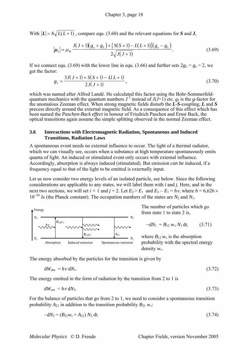
Let us now consider two energy levels of an isolated particle, see below. Since the following considerations are applicable to any states, we will label them with i and j. Here, and in the next two sections, we will set i = 1 and j = 2. Let E2 > E1 and E2 − E1 = hν, where h = 6,626 × 10−34 Js (the Planck constant). The occupation numbers of the states are N2 and N1.

The number of particles which go from state 1 to state 2 is,

E2

E1

Energy

N2

N1Absorption Induced emission Spontaneous emission

hν B12ρν

B21ρν A21

−dN1 = B12 wν N1 dt, (3.71)

where B12 wν is the absorption probability with the spectral energy density wν.

The energy absorbed by the particles for the transition is given by

dWabs = hν dN1. (3.72)

The energy emitted in the form of radiation by the transition from 2 to 1 is

dWem = hν dN2. (3.73)

For the balance of particles that go from 2 to 1, we need to consider a spontaneous transition probability A21 in addition to the transition probability B21 wν:

−dN2 = (B21wν + A21) N2 dt. (3.74)


Chapter 3, page 19

The probability A21 does not depend on external fields. The probability of an induced transition, however, does depend the external field. It is the product of the B coefficients with the spectral energy density wν of the external fields in the frequency range from ν to ν + dν. The spectral energy density wν has the units of an energy per volume and frequency. Instead of this quantity, the spectral beam density Lν is often used. Lν is the power in the frequency range ν to ν + dν that is emitted per unit area in a cone of solid angle Ω =1. A solid angle Ω =1 would mean that 1 m2 is cut out of the total surface area of 4π m2 of a sphere with a radius of 1 m. The aperture angle of the cone is about 66°. In a vacuum, where the speed of light is c0 it holds that Lν = wν c0/4π. (3.75) B12 and B21 are the Einstein coefficients for absorption and induced emission. With the help of these coefficients Albert Einstein could find a simple and secure proof of the radiation law in 1917. The radiation law was discovered at the end of 1900 by Max Planck through an interpolation (of the behaviour of the second derivative of the entropy with respect to the energy) between Wien’s radiation law and Rayleigh Jeans radiation law. Einstein’s derivation starts with a closed cavity in a heat bath at the temperature T. Because of equilibrium, we have for two arbitrary states between which transitions occur that the number of absorbed and emitted quanta of energy must be equal. wν is in this case the spectral energy density of a black body, labelled with ρν. From (A21 + B21 ρν) N2 = B12 ρν N1 it follows that

NN

BA B

2

1

12

21 21=

+ρ

ρν

ν. (3.76)

On the other hand, Boltzmann statistics can be applied to this system:

NN

gg

E EkT

gg

hkT

2

1

2

1

2 1 2

1

= −−⎡

⎣⎢⎤⎦⎥

= −⎡⎣⎢

⎤⎦⎥

exp exp ν . (3.77)

k refers to the Boltzmann constant, and h is Planck’s elementary quantum of action. The statistical weights, g1,2 are from now on set to g1 = g2 =1, i.e. a degeneration of the energy levels will not be considered. With equations (3.76) and (3.77) we arrive at:

ρν ν=−

A

B BhkT

21

12 21e . (3.78)

In equ. (3.78), no statement about the relationship between B12 and B21 is made. If we make the plausible assumption that as T → ∞ , ρν → ∞ must also hold, we get from equ. (3.78) the relation that B12 = B21.


Chapter 3, page 20

For the determination of the relationship between A21 and B21 the radiation law from 1900 stated by Lord Rayleigh and James Hopwood Jeans is used. In the low frequency range (hν « kT), equ. (3.78) should fulfill the Rayleigh-Jeans law

ρν = 8 2

03

π ν kTc

, (3.79)

which we will derive later using classical statistics. With exp (hν/kT) ≈ 1 + hν/kT and hν « kT , we get from equ. (3.78) by setting B12 = B21

ρν =A kTB h

21

21 ν. (3.80)

From equations (3.79) and (3.80) it follows for arbitrary relationships between hν and kT that the valid relationship between the spontaneous and induced transition coefficients is

AB

hc

21

21

3

03

8=

π ν. (3.81)

Equation (3.81) put into (3.78) leads us to the famous Planck radiation law:

ρπ ν

ν =8 3

03

hc

1

1ehkTν

− . (3.82)

If we use the wavelength dependent energy density ρλ dλ instead of the frequency dependent energy density ρν dν , we conclude that in a vacuum:

ρπλλ =

8 05

hc

1

10

ehckTλ −

. (3.83)

using the relationships ν = c0/λ and dν = −c0/λ2 dλ. The Rayleigh-Jeans law, which applies when hν « kT, is used in Einstein’s derivation of the Planck radiation law. Other radiation laws were not used, but can be presented as results of the Planck radiation law in the frame of the Einstein derivation: For hν » kT it holds that exp (hν/kT) » 1, and we get from equ. (3.82) as a special case the Wien radiation law, derived by Wilhelm Wien in 1896 (up to the factors later determined to be 8πh/c0

3 and h/k):

ρπ ν

ν =8 3

03

hc

e−

hkTν

. (3.84)


Chapter 3, page 21

If we construct the first derivative of equ. (3.83) with respect to the wavelength and set this to zero, we get the a maximum of the spectral energy density of the black body at λmax. The wavelength follows the relationship

λmaxT = const. = h c

k0

4 9651, = 2,8978 mm K (3.85)

and describes a displacement of the maximum of the intensity distribution to shorter wavelengths as the temperature increases. (The number 4,9651 is the zero point of the derivative, rounded to the nearest decimal. Because of this, the number 2,8978 is also rounded). This law, derived by Wien in 1893, is known as Wien’s displacement law. It was the basis of his thoughts for the first form of his radiation law. At 300 K, the maximum of the radiation of a black body is in the infrared at approx. 10 μm. Only at about 4000 K does it move into the visible spectrum. From equations (3.83) and (3.85) we get the law ρλ

max = const. · T 5 (3.86) for the energy density in the range of the maximum. For completeness, mention also Josef Stephan’s empirical law of 1878, later clarified with thermodynamics by Ludwig Eduard Boltzmann. It is known as the Stefan-Boltzmann law, and is arrived at by integrating equ. (3.83):

= T 4 ρ λλd0

∞

∫815

6 4

03 3

π kc h

= σ T4 . (3.87)

The total radiation of the black body is proportional to the fourth power of the temperature. We stress again that in the above equations, energy densities are used. To convert to the often used beam density, use equ. (3.75). For example, the factor σ in equ. (3.87) is changed into 2π5 k4/(15c0

2 h3) ≈ 5,67 × 10−8 W m−2 K−4, if we use Lλ instead of ρλ.

0 10000 20000 30000 400000

2

4

6

8

10

12

Planck 3000 K

Wien 5000 K

Planck 5000 K Rayleigh-Jeans 5000 K

ρν/

10−1

6 Js m

−3

wave numbers / cm−1

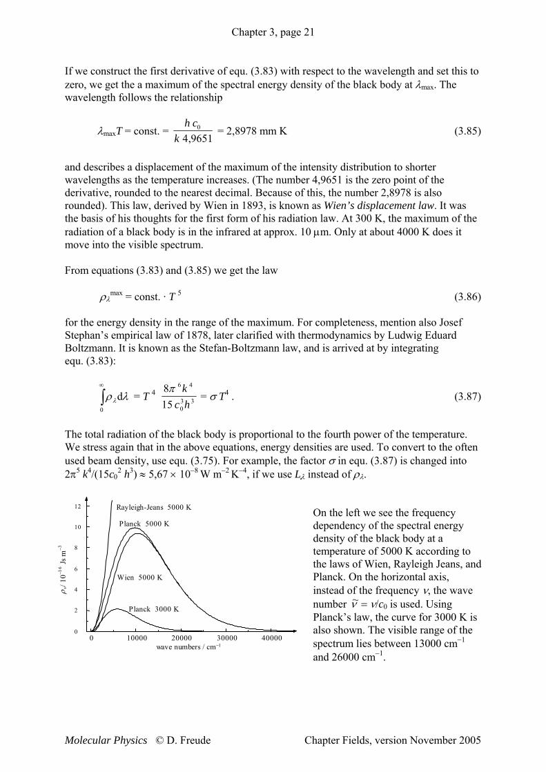
On the left we see the frequency dependency of the spectral energy density of the black body at a temperature of 5000 K according to the laws of Wien, Rayleigh Jeans, and Planck. On the horizontal axis, instead of the frequency ν, the wave number ~ν = ν/c0 is used. Using Planck’s law, the curve for 3000 K is also shown. The visible range of the spectrum lies between 13000 cm−1 and 26000 cm−1.


Chapter 3, page 22

If we use the Einstein coefficients, we get the relationship between spontaneous and induced emission probabilities by rewriting equ. (3.80):

A

BhkT

21

21 ρν

ν= . (3.88)

At a temperature of 300 K, the equilibrium between both probabilities is at ν = k·300 K / h ≈ 6,25 × 1012 Hz, and ~ν = 208 cm−1 or λ = 48 μm, in the far infra red. That is true for black body radiators, which are best made using a tempered cavity whose radiation escapes through a small hole. In a laser, much higher beam densities escape than in a black body. By concentrating the beam density in an extremely small frequency spectrum, the induced emission in a laser dominates, even in higher frequency ranges.

To expand upon the relationship of spontaneous to induced emission, we introduce characteristic vibrations, or modes. Thereby we can use either the photon picture or the wave picture in a closed cubic cavity with parallel mirrors. In the photon picture, a photon is reflected back and forth between the mirrors. In the wave picture, the field strength of a standing wave disappears at the edge of the cavity. For that reason, we have to use a whole number multiple of λ/2 for the distance between the mirrors L. You can find in other textbooks a further wave picture which uses a wave moving back and forth instead of a standing wave. In that case, the distance between the mirrors L has to be a whole number multiple of λ, and the wave vector k determined from the different positive and negative directions of propagation where k = (2π/L) (nx, ny, nz) for positive and negative values of ni. In our further considerations, we use the picture of a standing wave in a vacuum. The wave vector for an arbitrary standing wave in a cube of edge length L is:

k = πL

(nx, ny, nz) (3.89)

where ni is a positive whole number. It is valid with |k| = 2π/λ

ν = ωπ2

= c0

λ = |k|

c0

2π =

cL0

2 n n nx y

2 2+ + z2 . (3.90)

A vector potential A can be derived from the sum of all modes where

A = sin (kjr −ωjt). (3.91) a jj

∑The vector amplitudes aj represent time dependent vectors and every index j and every wave vector kj stand for a certain combination of (nx, ny, nz). We assume that A is the vector potential of the electromagnetic field and set divA = 0. With that it holds for every value of j the scalar product kj aj = 0. The wave vector is therefore perpendicular to the amplitude vector. The wave is transversal and can be represented as a linear combination of two linearly polarized waves. For this reason every vector kj has two characteristic vibrations, or modes (or states).

Due to the wave vector definition in equ. (3.89), the k vector can be represented by a point in a three dimensional k-space. The difference between this space and our normal 3-D space is that it only contains points for whole number values of nx, ny and nz. The number Δn of possible values of k in the intervals Δkx, Δky and Δkz is equal to the product of Δnx Δny Δnz.


Chapter 3, page 23

With of ki = (π/L) ni we get

Δn = L3

3π Δkx Δky Δkz. (3.92)

The number of points between |k| and |k| + Δ|k| is equal to the volume of a spherical shell. Since only positive values of ni are considered, only the relevant octant must be considered (1/8 of the total volume of the spherical shell):

Δn = L3

3

48ππ

|k|2 Δ|k|. (3.93)

If we additionally take into account that for every vector, the two polarization possibilities of the wave give two modes, then the number of different modes per unit volume is

ΔnL3 =

12π

|k|2 Δ|k|. (3.94)

The transition from differences (Δ) to differential quantities (d) occurs when we replace Δn/L3 with n(ν) dν (the number of modes per unit volume in the differential frequency range) and Δ|k| by d|k| having considered |k| = 2πν/c0. With that we get

n(ν) dν = 8 2

03

πν νdc

. (3.95)

Here we make an insertion, in order to derive the radiation law after Rayleigh. The energy of a classical oscillator is the sum of potential and kinetic energy which amounts kT for each oscillation. This gives ρν = n(ν) kT and we obtain the Rayleigh-Jeans law

ρν = 8 2

03

π ν kTc

. (3.79)

Coming back after the (Rayleigh-)insertion we we put equ. (3.81) into (3.95). Then the relationship of the emission coefficients is

AB

21

21= n(ν) hν. (3.96)

By expanding this relationship with the spectral energy density wν the relationship of the induced to spontaneous emission probability follows

( )B w

Aw

n h21

21

1 1νν ν ν

= =

=×

×=

photon a ofenergy 1

modes ofnumber frequencyvolume

frequencyvolumephotons ofenergy N (3.97)

modes ofnumber

photons theofnumber N= .

Related to a single mode, this means that: the relationship of the induced to the spontaneous emission probability is equal to the number of photons in this mode for an arbitrary mode. With that the representation of the induced emission in the diagram at the beginning of this chapter has the following explanation: Induced emission occurs when a photon with the appropriate energy meets a mode containing many photons.


Chapter 3, page 24

With the previously derived relationship, an easy consideration of the interaction of electromagnetic radiation with atoms, molecules, and solid bodies is possible. Although we will use quantum theoretical results in our considerations, we will not get into the derivations of these results. In the case at hand, we can replace the exact quantum theoretical descriptions with semi-classical derivations. Let us consider a dipole, for example an antenna whose charge distribution changes with the circular frequency ω. The time dependent electric dipole moment is

μ(t) = μ cosωt. (3.98)

The radiant power of a classical (spontaneous) radiating dipole follows from electrodynamics as the average radiated power. The time average of a periodic function f is represented by

f .

( )Pc

t

t cem

2d

d=

⎡

⎣⎢⎢

⎤

⎦⎥⎥

=14

23 10 0

3 2

24 2

0 03πε

ωπε

μ μ2

, (3.99)

cf. e. g. Landau/Lifschitz II, p. 205. In the transition from the middle to the right part of the equation, the average cos2ωt = ½ was used.

The correspondence principle touches on the fact that quantum mechanical systems for high quantum numbers obey the laws of classical physics. Though that it was possible to determine selection rules and make statements about intensity and polarisation of spectral lines. By using this principle, we can take the following path: put into equ. (3.99) the operator for the dipole moment μ = qr , in which q represents the absolute value of the charges separated by the distance r. The vector µ is replaced by vector operator $μ or q which is multiplied by two. The factor two is introduced because of the two possibilities of the electron spin. With this operator, it follows that the dipole moment of a transition from state 2 to state 1 is:

$r

, (3.100) M r21 2 1= ∗∫q ψ ψ τ$ d

where ψ1 is the wave function of state 1 and ψ2* is the complex conjugated function of state 2. The integration is done over all variables of the functions (in this case over space). From that we get the expectation value of the power from equ. (3.99):

Pc21

4

0 03 21

2

3=

ωπε

M . (3.101)

Since is a vector operator, M21 is also a vector: |M21|2 = $r M M Mx y212

212

212

z+ + .

For a spontaneously radiating dipole, we get the transition probability

2213

00

332

21300

321

21 316

3MM

hcchP

Aε

νππε

ων

===h

. (3.102)

Using the relation A21 /B21 = 8 hν3/c03, equ. (3.81), and equ. (3.102) the Einstein coefficient

of the induced emission can be calculated:

2212

0

3

21 32 M

hB

επ

= . (3.103)


Chapter 3, page 25

Equations (3.102) and (3.103) describe the relationship of the emission coefficients B21 and A21 to the absorption coefficients B12 (= B21) with the dipole moment of the transition M21, which is connected to the wave functions of the states under consideration by equ. (3.100). Since the particles to be studied are characterised by these wave functions, equations (3.102) and (3.103) represent an important basis of the interaction of particles with electromagnetic radiation. They are the basis of many spectroscopic experiments. The dipole moment M of the transition is rarely calculated. Even without calculation, we can determine whether M is zero or has a finite value from the symmetry considerations of chapter 4 (forbidden and allowed transitions).

3.7 Lines and Band Intensities in Optical Spectra Pierre Bouguer determined in 1726 that the attenuation of a beam of light in an absorbing medium is proportional to the intensity of the beam and the length of the medium. Johann Heinrich Lambert described in 1760 this fact with an equation and August Beer found in 1852 through absorption measurements on rarefied solutions that the transmittance of a material with a constant cross section only depends on the amount of material through which the light shines. These realizations led to the fundamental law for quantitative optical spectroscopy, which is named after the last, the last two, or all three discoverers. If the light intensity transmitted by an absorbing layer is I = D I0, then it follows for the logarithm of the transmittivity and the transmittivity

log10

II 0

= − εν cM d and D = exp (− εν cM d ln 10). (3.104)

The εν in the Beer law is the frequency dependent molar extinction coefficient and d is the thickness of the layer of the substance (normally in cm). cM is the concentration of the absorbing substance, normally given in Mol per Litre and often called the molarity. The dimension of εν is volume × mole−1 × thickness of layer−1, where the usual units are mole/litre and cm for the thickness of the layer, thus 1000 cm2 mol−1. The SI unit of m2 per mole (m2 mol−1), which is 10 times larger, is rarely used. Unfortunately, the molar extinction coefficient is often given with no units at all, even though it has dimensions, in contrast to the extinction εν cM d. There is also the possibility for confusion by the usage of the natural extinction coefficient εν

n, where in equ. (3.104) in place of the decade logarithm the natural logarithm is used. It is valid that εν

n = εν ln 10 ≈ εν 2,03.

The empirically introduced extinction coefficient depends on the imaginary part of the index of refraction, which describes the damping of the electric field as it passes through a medium. Since the radiant energy is proportional to the square of the amplitudes of the field strength, see chapter 2.1, from the comparison equations (3.43) and (3.104), this relation follows:

2n"ω/c0 = ενn cM = mν , (3.105)

in which ενncM is the natural extinction module mν (extinction per unit length). Equation

(3.41) inserted into (3.105) shows that the extinction near the resonance is represented by a Lorentz curve.


Chapter 3, page 26

For practical applications it is advantageous to measure the integral extinction of a line or band. For the derivation of the corresponding relation we will limit ourselves to linear absorption. In that case, for a beam incident perpendicular to the surface F, that the incident spectral radiant intensity I = c0 wν F. The absorbing spectral intensity follows from the relation I = I0 exp(−mν x), see equations (3.104) and (3.105), dI = c0 wν F mν dx. (3.106) With F as unit area we get the spectral absorbed intensity Iabs per unit volume after integration of the x-coordinate over the unit length: Iabs = c0 wν mν , (3.107) which is a function of the frequency. In the frequency range of a line (or band), the spectral energy density wν of the incident electromagnetic wave can be considered constant. Through that we get after integration over the frequency range of a line the integral absorbed intensity, which is a power density:

swcmwcmwct

w dd

dd

0

end line

begin line0

end line

begin line0

absννννν νν === ∫∫ . (3.108)

The integral absorption coefficient, introduced here and the integral extinction module s can be rewritten as integral extinction coefficient after division by the concentration of the substance. This is more useful for practical applications than the frequency dependent value. We must of course be careful not to integrate over the whole spectrum but rather over the line or band under consideration. The netto rate of the transitions i → k, see equ. (3.71), is Bik wν Ni in a transition between non degenerate energy levels with Ek > Ei and Nk « Ni. For every transition, the energy hνik is absorbed. Ni is the number of states per unit volume. We then have for the absorbed power per unit volume:

d

dabswt

= hνik Bik wν Ni. (3.109)

With equations (3.108), (3.109) and (3.103) it follows that

s = h B N

cik ik iν

0 = 2

00

3

32

ikiik

hcN M

ενπ . (3.110)

These equations combine the integral absorption coefficient with the dipole moment of the transition, i.e. a parameter determined by an experimentally measured spectrum with the quantum mechanical expectation value. The later is not easy to calculate and depends on the symmetry of the molecule or solid body building block and perturbations of this symmetry. For this reason, quantitative statements from optical spectra are problematic.


molecules in electric and magnetic fields

Documents