Molecular models for the hydrogen age:

Hydrogen, nitrogen, oxygen, argon and water

Andreas Koster,† Monika Thol,‡ and Jadran Vrabec∗,†

†Lehrstuhl fur Thermodynamik und Energietechnik, Universitat Paderborn,

33098 Paderborn, Germany

‡Lehrstuhl fur Thermodynamik, Ruhr-Universitat Bochum, 44801 Bochum, Germany

E-mail: jadran.vrabec@upb.de

Phone: +49-5251 60-2421. Fax: +49 5251 60-3522

Abstract

Thermodynamic properties including the phase behavior of all mixtures containing

hydrogen, the main components of air, i.e. nitrogen, oxygen and argon, and water

are of particular interest for the upcoming post-carbon age. Molecular modeling and

simulation, the PC-SAFT equation of state as well as sophisticated empirical equations

of state are employed to study the mixture behavior of these five substances. For this

purpose, a new force field for hydrogen is developed. All relevant subsystems, i.e.

binary, ternary and quaternary mixtures, are considered. The quality of the results is

assessed by comparing to available experimental literature data, showing an excellent

agreement in many cases. Molecular simulation, which is the most versatile approach in

general, also provides the best overall agreement. Consequently, this contribution aims

at an improved availability of thermodynamic data that are required for the hydrogen

age.

1

Keywords

Hydrogen age, Molecular modeling and simulation, Equation of state, PC-SAFT

1 Introduction

Even in the international political arena, it is now globally accepted that human civilization

must switch from fossil to renewable energy sources because atmospheric pollution threatens

our climate1. Much less attention is being paid in these discussions that fossil fuel resources

were always also a potent driver of conflict basically from the onset of industrialization2,3.

An attractive alternative energy carrier is hydrogen (H2) that has major advantages over

carbon-based fuels. H2 can be used in all kinds of combustion processes and can reduce

harmful carbon dioxide (CO2) emissions to a minimum. An approach with an even wider

impact, avoiding thermal energy that is associated with the Carnot limit, is the usage of fuel

cells to directly convert chemical energy from H2 with ambient air into electric energy and

water. 1 kg H2 contains 33.3 kWh of chemical energy, if the lower heating value of H2 is

employed. Modern electrolysers require an electricity input of 52 kWh/kg on average, which

corresponds to an electrical efficiency of 64 %4. Since renewable energy sources, such as

wind or solar energy, are fluctuating in nature and need to be balanced, their excess power

may be employed for hydrogen production5.

Very prominent devices using H2 as a fuel both for combustion and for fuel cells were the

NASA space shuttles6. However, the whole classical transportation sector could in general

profit from fuel cells as Momirlan and Veziroglu6 point out. In 2016, over 100 fuel cell buses

for public transportation were in use worldwide7. More recently, first test runs with a new

fuel cell passenger train were performed8. There are, however, numerous other meaningful

approaches for the usage of H29. It may, e.g., be processed together with CO2 in a power

to gas approach and subsequently stored in the form of methane in widely available storage

facilities10. All of these techniques have in common that accurate thermodynamic data are

2

needed for their design and optimization.

Since experimental measurements alone do not keep up with the demand for thermo-

dynamic data, it must also be focused on other methods, which is the goal of this study.

Accordingly, the mixture behavior of five substances related to the hydrogen age, i.e. H2,

nitrogen (N2), oxygen (O2), argon (Ar) and water (H2O), is tackled with molecular modeling

and simulation, the PC-SAFT equation of state (EOS) as well as sophisticated empirical EOS

and compared to experimental data, if available. All relevant subsystems are described. Sev-

eral literature studies already dealt with some of these subsystems. Stoll et al.11 and Vrabec

et al.12 performed molecular simulation studies on binary mixtures related to dry air (N2 +

O2, N2 + Ar and Ar + O2), which were then used to predict cryogenic vapor-liquid equilibria

(VLE) of dry air (N2 + O2 + Ar)13,14. Furthermore, humid air (N2 + O2 + Ar + H2O) was

examined by Eckl et al.14. Related studies with a different objective, i.e. CO2 mixtures for

carbon capture and sequestration (CCS) and the like, were conducted by means of molecular

modeling and simulation by Vrabec et al.15 (N2 + O2 + CO2), Tenorio et al.16 (H2 + CO2)

and Cresswell et al.17 (binary mixtures of CO2 with H2, N2, Ar and O2). Moreover, several

studies employed the statistical associating fluid theory (SAFT) in its various forms or cubic

EOS to study mixtures containing CO218,19. Solubilities of binary aqueous systems (N2 +

H2O and H2 + H2O) were examined by Sun et al.20 with the SAFT-Lennard-Jones EOS.

Finally, empirical multiparameter EOS formulated in terms of the Helmholtz energy are

available, namely the GERG-200821 and a recently developed model for combustion gases

(EOS-CG)22. These EOS are typically very accurate in reproducing experimental data.

However, the EOS-CG unfortunately does not cover H2 and the GERG-2008 EOS does not

aim at cryogenic conditions. Consequently, a comprehensive study focusing on carbon-free

mixtures containing H2 is a necessity.

Different thermodynamic properties were considered in this work to describe a substantial

number of mixtures. Apart from VLE properties, like vapor pressure, saturated densities or

residual enthalpy of vaporization, also homogeneous density and solubility were studied. Sol-

3

ubility, i.e. Henry’s law constant, is typically relevant for mixtures in which one component

is only little soluble in the other, as it is the case for aqueous systems that are considered

in the present work. In the following sections, the employed models are described before

the results of this study are presented and discussed. Finally, a conclusion sums the present

work up.

2 Methodology

2.1 Modeling of pure fluids and mixtures

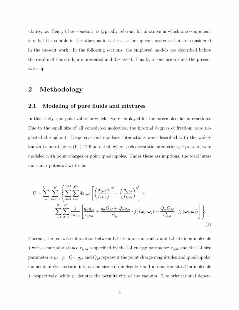
In this study, non-polarizable force fields were employed for the intermolecular interactions.

Due to the small size of all considered molecules, the internal degrees of freedom were ne-

glected throughout. Dispersive and repulsive interactions were described with the widely

known Lennard-Jones (LJ) 12-6 potential, whereas electrostatic interactions, if present, were

modeled with point charges or point quadrupoles. Under these assumptions, the total inter-

molecular potential writes as

U =N−1∑i=1

N∑j=i+1

SLJi∑

a=1

SLJj∑

b=1

4εijab

[(σijabrijab

)12

−(σijabrijab

)6]

+

Sei∑

c=1

Sej∑

d=1

1

4πε0

[qicqjdrijcd

+qicQjd +Qicqjd

r3ijcd· f1 (ωi,ωj) +

QicQjd

r5ijcd· f2 (ωi,ωj)

]}.

(1)

Therein, the pairwise interaction between LJ site a on molecule i and LJ site b on molecule

j with a mutual distance rijab is specified by the LJ energy parameter εijab and the LJ size

parameter σijab. qic, Qic, qjd and Qjd represent the point charge magnitudes and quadrupolar

moments of electrostatic interaction site c on molecule i and interaction site d on molecule

j, respectively, while ε0 denotes the permittivity of the vacuum. The orientational depen-

4

dence of the electrostatic interactions is considered through the trigonometric expressions

fx(ωi,ωj)23. Finally, the summation limits N , SLJ

x and Sex denote the number of molecules,

the number of LJ sites and the number of electrostatic sites, respectively.

The force fields for Ar, N2 and O2 were taken from the work of Vrabec et al.24. These force

fields were adjusted to experimental VLE data and it was shown that they are an adequate

choice for numerous fluid mixtures17,25–28. For H2O, the widely appreciated TIP4P/2005

force field29, which performs well for a large variety of thermodynamic properties30–32, was

employed.

The description of molecular hydrogen with semi-empirical force fields or other common

thermodynamic models, like EOS, is challenging. Due to its small mass, quantum effects

have to be taken into account. These effects have a strong influence on macroscopic ther-

modynamic properties, especially at low temperatures33. Therefore, a force field that was

adjusted to the VLE properties of hydrogen at low temperatures will lead to poor results us-

ing classical atomistic simulations at higher temperatures. Furthermore, molecular hydrogen

is anisotropic because of its two nuclei and its nonspherical charge distribution and typically

consists of ortho and para hydrogen with different quantum spin states34. Several authors

have been working on modeling H2 in the last decades, describing the intermolecular interac-

tions with a single LJ 12-6 site35, a LJ 12-6 site with an additional point quadrupole for the

anisotropic interactions36–38, or more complex force fields, which also account for many-body

polarization39. In this work, both a single site LJ force field, initially taken from Hirschfelder

et al.35 and subsequently adjusted to speed of sound and thermal (pV T ) properties of H2

at temperatures from 50 to 250 K, and one with an additional point quadrupole from Marx

and Nielaba36 were considered. All force field parameters are listed in Table 1. It should be

noted that point quadrupoles can easily be represented with a set of three point charges if

required40.

When describing mixtures, interactions between unlike molecules have to be taken into

account. The unlike dispersive and repulsive interactions between LJ site a of molecule i

5

Table 1: Parameters of the present molecular interaction force fields.

Interaction Site x y σ ε/kB q QA A A K e DA

Hydrogen AH2 0 0 3.0366 25.84Hydrogen B36

H2 0 0 2.9580 36.7 0.6369Nitrogen24

N 0 -0.5232 3.3211 34.897N 0 0.5232 3.3211 34.897Quadrupole 0 0 -1.43971

Oxygen24

O 0 -0.4850 3.1062 43.183O 0 0.4850 3.1062 43.183Quadrupole 0 0 -0.80811

Argon24

Ar 0 0 3.3952 116.79Water29

O 0 0 3.1589 93.2H 0.5859 0.7570 0.5564H 0.5859 -0.7570 0.5564M (Mid Point) 0.1546 0 -1.11281 The quadrupole is oriented along the molecular axis.

6

and LJ site b of molecule j were specified with the modified Lorentz-Berthelot combination

rule

σijab =σiiaa + σjjbb

2, (2)

and

εijab = ξ(εiiaaεjjbb)1/2. (3)

The temperature independent binary interaction parameter ξ was adjusted to achieve a bet-

ter representation of experimental mixture data. This adjustment can most favorably be

done on the basis of one experimental data point of the vapor pressure at an equimolar com-

position because the binary interaction parameter ξ has the strongest influence under these

conditions41. If a binary interaction parameter is available, mixtures with more than two

components do not require further optimization because of pairwise additivity. The unlike

electrostatic interactions were treated straightforwardly according to the laws of electrostat-

ics and do not require any binary interaction parameters.

2.2 Simulation details

Throughout, Monte Carlo (MC) sampling42 with the release 3.0 of the molecular simula-

tion program ms243–45 was used to generate the thermodynamic data presented here. A

cutoff radius of 15 A was employed. The LJ long-range corrections, considering the interac-

tions beyond the cutoff radius, were calculated with the angle-averaging method of Lustig46,

whereas long-range electrostatic interactions were considered by means of the reaction field

method23. Statistical uncertainties of the simulation data were estimated by averaging over

a sufficiently large number of uncorrelated blocks consisting of 5000 MC cycles each47. Three

different molecular simulation workflows were employed:

1. VLE calculations were carried out with the grand equilibrium method48. This approach

consists of two independent and subsequent simulation runs for the two phases in

equilibrium. For the liquid phase, 864 particles were sufficiently equilibrated and then

7

sampled for 106 production cycles in the isobaric-isothermal (NpT ) ensemble. One

such cycle consists of M/3 · 864 translational and rotational as well as one volume

move attempt, where M is the number of molecular degrees of freedom. The chemical

potential of every component in the liquid phase was sampled with Widom’s test

particle insertion49. From the results of this run, the chemical potential as a function

of pressure µi(p) at constant liquid composition was approximated by a Taylor series

expansion. This function was used in the subsequent pseudo grand canonical (µV T )

ensemble simulation of the vapor phase to sample the vapor pressure. For this run 1000

particles were used, which were thoroughly equilibrated in advance. The production

phase was 2·105 MC cycles, which consisted of M/3·1000 particle displacements as well

as three insertion and three deletion attempts. More details on the grand equilibrium

method can be found elsewhere48.

2. The Henry’s law constant Hi was sampled in the NpT ensemble in the saturated liquid

state of the solvent, i.e. H2O, using 1000 particles. Hi is closely related to the chemical

potential at infinite dilution µ∞i50

Hi = ρskBT exp(µ∞i /(kBT )), (4)

wherein ρs is the saturated liquid density of the solvent, T the temperature and kB

Boltzmann’s constant. The chemical potential at infinite dilution was obtained with

Widom’s test particle insertion49. For this purpose, the mole fraction of the solute

was set to zero such that only test particles were inserted into the pure solvent. The

simulation runs consisted of 3 · 106 MC cycles, i.e. 2 · 105 equilibration and 2.8 · 106

production cycles.

3. pV T calculations for homogeneous bulk phases were carried out in the NpT ensemble

using 864 particles. After a thorough equilibration, the density ρ was sampled over 106

production cycles. Again, one cycle consisted of M/3 · 864 translational and rotational

8

as well as one volume move attempt.

2.3 PC-SAFT equation of state

In addition to atomistic molecular simulation, the perturbed-chain statistical associating

fluid theory (PC-SAFT) EOS was employed. It is also based on theoretical considerations

(i.e. intermolecular interactions) and can therefore, like atomistic molecular simulation, be

used in cases where only little experimental data are available. Since Gross and Sadowski

developed the PC-SAFT EOS in 200151, several improvements were implemented. Having

only three pure component parameters in its initial form, Gross and Sadowski added a

term to account for association in 2002 that requires two additional parameters52. Further

developments involved e.g. Helmholtz energy contributions of polar interactions53–55 or cross

associations56. Numerous studies showed that the PC-SAFT EOS is a powerful predictive

approach to mixture behavior19,57,58.

Since pairwise additivity is assumed, modeling mixtures in the PC-SAFT framework is

reduced to the description of unlike chain interactions. This was done here with the modified

Lorentz-Berthelot combination rule, cf. Eqs. (2) and (3), with a slightly different expression

for the unlike energy parameter

εij = (1− kij)(εiεj)1/2, (5)

wherein kij is a temperature independent binary parameter.

The pure component parameters of the PC-SAFT EOS were taken from the litera-

ture18,51,59,60, cf. Table 2. It has to be noted that H2 is modeled as a spherical molecule

having similar parameters as the force field developed in this work. VLE properties and

homogeneous densities can be calculated straightforwardly with the PC-SAFT EOS. Solu-

bilty data, i.e. the Henry’s law constant, can be obtained with the PC-SAFT EOS through

the fugacity coefficient of a solute at infinite dilution. This approach was, e.g., utilized by

9

Vins and Hruby61 for the solubility of N2 in refrigerants. Note that, these systems exhibit

solubilities which are orders of magnitude larger than those of the present aqueous systems.

The solubility of H2, N2, O2 and Ar in H2O could not be reproduced satisfactorily with

PC-SAFT EOS, applying even more complex methods. Various H2O models with several

association schemes (2B, 4C), permanent polarities for both H2O and the solutes as well as

induced association as described by Kleiner and Sadowski56 led only to little improvement.

Therefore, modeling the solubility of the present aqueous mixtures with the PC-SAFT EOS

was omitted in the main body of this study. However, some solubility results from the

PC-SAFT EOS are shown in the supporting information.

Table 2: Pure component parameters of the PC-SAFT EOS.

Component M m σ ε/kB κAiBi εAiBi/kBg/mol - A K - K

Hydrogen59 2.016 1 2.9150 37.00 - -Nitrogen51 28.010 1.2053 3.3130 90.96 - -Oxygen18 32.050 1.1217 3.2100 114.96 - -Argon51 39.948 0.9285 3.4784 122.23 - -Water60 18.015 2.5472 2.1054 138.63 0.2912 1718.2

2.4 Peng-Robinson equation of state

Empirical EOS are typically used to correlate thermodynamic data from experiment, offering

inter- and extrapolation capabilities between and beyond these data. Being simple and often

considered to be accurate enough to cover a wide range of thermodynamic properties, the

Peng-Robinson EOS62 is one of the most widely used cubic EOS63. It is given by

p =RT

v − b− a(T )

v(v + b) + b(v − b), (6)

with pressure p, universal gas constant R, molar volume v and two substance-specific pa-

rameters

10

a(T ) = 0.45724(RTc)

2

pcα(T ), (7)

and

b = 0.07780RTcpc

. (8)

Therein, Tc and pc are the critical temperature and pressure. Numerous alpha functions

α(T ) were proposed in the literature, e.g. by Soave64, Peng and Robinson62, Mathias and

Copeman65 or Stryjek and Vera66. However, the best overall results for the present fluid

mixtures were achieved here with the alpha function of Twu et al.67

α = (T/Tc)N(M−1)exp(L(1− (T/Tc)

NM)), (9)

wherein L, M and N are substance-specific parameters, which are usually fitted to pure

component vapor pressure data. Table 3 lists the numerical values for L, M and N for the

pure substances considered in the present work68.

Table 3: Pure component parameters of the Twu-Bluck-Cunningham-Coon alpha functionaccording to the Dortmund data base68.

Component Tc pc L M NK MPa - - -

Hydrogen 33.2 1.297 0.926823 5.127460 0.084639Nitrogen 126.2 3.394 0.329500 0.882750 1.052080Oxygen 154.6 5.046 0.550161 0.933432 0.693063Argon 150.8 4.874 0.557990 0.998454 0.669817Water 647.3 22.048 0.44132 0.87340 1.75990

Mixtures can be represented by applying mixing rules to EOS. A standard approach,

which is commonly used in conjunction with the Peng-Robinson EOS, is the quadratic Van

der Waals one-fluid mixing rule67. Following this rule, the two substance-specific parameters

are replaced by

11

am =∑i

∑j

xixjaij, (10)

and

bm =∑i

xibi, (11)

wherein

aij = (1− kij)(aiaj)1/2. (12)

In this work, the Peng-Robinson EOS was not only used to determine vapor pressure and

composition of the coexisting phases but also homogeneous density and residual enthalpy of

vaporization data. For details on these calculations in the context of cubic EOS, the reader is

referred to the standard literature69. In analogy to the approach described for the PC-SAFT

EOS, it was attempted to calculate fugacity coefficients in order to obtain the Henry’s law

constant. Unfortunately, it was not possible to achieve even qualitative agreement with the

experimental data. Therefore, solubility of the aqueous systems was not described with the

Peng-Robinson EOS in the main body of this study. However, some solubility results from

the Peng-Robinson EOS are shown in the supporting information.

2.5 Multiparameter Helmholtz energy equations of state

It is widely known that empirical multiparameter EOS, which are most often explicit in

terms of the Helmholtz energy, are among the most accurate models for thermodynamic

properties, if the underlying experimental data base is of high quality and sufficiently large.

These requirements are met for several pure substances, like H2O70 or CO2

71, where the

uncertainty of the resulting empirical EOS is comparable to the error of the underlying

experiments. Unfortunately, very few pure substances were measured that thoroughly. When

considering mixtures, the necessary size of an experimental data base is even larger, since

the mixture composition appears as an additional independent variable.

12

To date, only few empirical Helmholtz energy EOS are available for mixtures, among the

most popular ones are the GERG-2008 EOS21 and the EOS-CG22. Both of these EOS were

adjusted to experimental binary mixture data and are able to predict the mixture behavior

of higher order mixtures assuming pairwise additivity. The GERG-2008 EOS was mainly

developed for the thermodynamic properties of natural gases21 and covers 21 components,

including the five present ones. Although the EOS-CG covers only six components, i.e.

CO2, H2O, N2, O2, Ar and CO, it is also highly relevant here because it aims at humid

combustion gases and humid or compressed air22. Consequently, the EOS-CG serves in this

work as a reference for binary mixtures without H2, whereas the GERG-2008 EOS was seen

as a reference for systems containing H2.

3 Results and discussion

The VLE behavior of all employed models was evaluated on the basis of vapor pressure,

saturated densities and residual enthalpy of vaporization

∆hresvap = hresliq − hresgas = (hliq − hidealliq )− (hgas − hidealgas ). (13)

Additionally, homogeneous density and Henry’s law constant data are presented. Binary,

ternary and quaternary mixtures are discussed under conditions where experimental data

are available for assessment. Typically, three experimental isotherms from the literature

were taken to study the VLE behavior of binary mixtures. Attention was paid to selecting

more than one experimental data source to assess the validity of any single measurement

series. Along with a large temperature range, it was also aimed at a large composition range.

Experimental pvT data were selected to allow for an extrapolation of the employed models

to extreme conditions. An equimolar composition was preferred for binary pvT data because

this implies that unlike interactions have the strongest influence. If possible, supercritical

”liquid-like” (at high density) and supercritical ”gas-like” (at low density) states were taken

13

into account. Deviations were evaluated using the mean absolute percentage error (MAPE)

to a reference value (experimental or multiparameter EOS)

MAPE =100

n

n∑i

∣∣∣∣Xmodel,i −Xref,i

Xref,i

∣∣∣∣ , (14)

where n is the number of data points and X is a given thermodynamic property.

In cases where binary mixture models had to be adjusted to experimental data, only

a single temperature independent parameter was allowed, cf. section 2. For molecular

simulation, the binary interaction parameter ξ was either adjusted to one experimental

vapor pressure data point at some intermediate temperature close to equimolar composition

or, in the case of the aqueous systems, to reproduce experimental Henry’s law constant data

at T ≈ 320 K because numerous measurements are available around this temperature. The

adjustment of kij for the Peng-Robinson and the PC-SAFT EOS was carried out with the

least squares method using the available experimental vapor pressure data.

Some of the binary mixtures presented here, namely N2 + O2, N2 + Ar and Ar +

O2, were already studied by our group. Therefore, the binary interaction parameter ξ for

these mixtures was taken from that preceding work11,12. All binary parameters are listed in

Table 4. Higher order mixture data were not considered for adjustment because all of the

present models assume pairwise additivity. The numerical molecular simulation data and

the associated statistical uncertainties can be found in the supporting information. It has

to be noted that statistical uncertainties are only shown in the figures below if they exceed

symbol size.

3.1 Binary vapor-liquid equilibria

The fluid phase behavior of H2 + N2 is shown in Fig. 1 for three isotherms. For better visi-

bility, the diagram was separated, showing mixture data from molecular simulation obtained

with the present H2 force field (top) and the literature force field36 (center), respectively.

14

Table 4: Binary parameters for molecular models ξ, Peng-Robinson EOS kij and PC-SAFTEOS kij.

Mixture ξ Ref. kij (PR EOS) kij (PC-SAFT EOS)Hydrogen A / B + Nitrogen 1.08 / 0.88 -0.0878 0.1248Hydrogen A / B + Oxygen1 1 / 1 0 0Hydrogen A / B + Argon 1.06 / 0.895 -0.1996 0.0962Hydrogen A / B + Water 1.52 / 1.05 -1.4125 0.0500Nitrogen + Oxygen 1.007 11 -0.0115 -0.0030Nitrogen + Argon 1.008 12 -0.0037 -0.0065Nitrogen + Water 1.07 -0.0501 0.1198Oxygen + Water 1.00 - -Argon + Oxygen 0.988 12 0.0139 0.0086Argon + Water 1.05 - -1 Data for this binary mixture were predicted without assessment and are thuspresented in the supporting information only.

Additionally, the relative volatility

α =yi/xiyj/xj

, (15)

is depicted (bottom). Sufficient experimental data are available to validate the performance

of the models. This mixture shows a two-phase region that is typical if one of the components

is supercritical. Among the EOS correlations, the Peng-Robinson EOS exhibits the best

agreement with the experimental data, both in the saturated liquid and vapor, which also

leads to a good agreement for the relative volatility. The PC-SAFT EOS overestimates

the critical point and also shows an inadequate slope for the saturated liquid line at 83.15

K. None of the two empirical multiparameter EOS are shown in Fig. 1 because (a) H2 is

not implemented in the EOS-CG and (b) the GERG-2008 EOS yields a false liquid-liquid

equilibrium phase separation at 83.15 K and strongly overestimates the pressure for T >

83.15 K. However, cryogenic H2 mixtures were not the main focus during the development

of the GERG-2008 EOS and its normal range of validity in temperature is specified as 90

to 450 K21, which means that the lowest isotherm is an extrapolation. More details on

the performance of GERG-2008 EOS in case of H2 mixtures are shown in the supporting

information. Comparing the two H2 force fields, the present one shows a better agreement,

15

cf. Fig. 1 (bottom). Especially at T = 83.15 K on the saturated liquid line, the use of the

force field of Marx and Nielaba36 leads to an underestimation of the vapor pressure by about

9% when compared to the Peng-Robinson EOS.

Fig. 2 shows saturated densities (top) and residual enthalpy of vaporization (bottom)

for H2 + N2 for the same isotherms. Typically, there are no experimental mixture data

available for these properties. For the reasons discussed above, no empirical multiparameter

EOS results are shown. Cubic EOS, especially in their simple forms, often tend to yield a

poor representation of the saturated liquid density63, which can also be observed for this

system. The saturated liquid density at 83.15 K of pure N2 was overestimated by about 3.5

mol/l, which corresponds to a deviation of 13 % when compared to the other models and

the reference EOS for pure N276. For both properties, the two H2 force fields lead to quite

similar results.

VLE properties of H2 + Ar are depicted in Fig. 3. The separation of these diagrams into

sub-diagrams was done in analogy to H2 + N2. When compared to H2 + N2, this system

shows a similar shape of the phase envelope, but the vapor pressure is higher by about a

factor of two at the same temperature and H2 mole fraction. The solubility of H2 in liquid

Ar is thus lower than in liquid N2. The agreement between the Peng-Robinson EOS, the

molecular simulation data on the basis of the present H2 force field and the experimental

data is very satisfactory for the saturated liquid line. On the saturated vapor line, especially

for lower temperatures, deviations of all employed models to the experimental data can

be observed. This finding is validated by the relative volatility representation, cf. Fig. 3

(bottom). The PC-SAFT EOS is again characterized by an inadequate slope of the saturated

liquid line and yields a critical line which is higher than expected. At lower temperatures,

the molecular simulations with the literature force field for H2, cf. Fig. 3 (center), show

a similar behavior. For the same reasons as discussed before, the GERG-2008 EOS is not

shown here. Saturated densities and residual enthalpy of vaporization data for H2 + Ar are

not discussed in detail because they are quite similar to H2 + N2. The reader is referred to

16

�������������

�

� � �� �� � �� ��

�

�

������

�����������

�� �� � �� �� �

�������

�

�

�

�

��

������

�

������

����

��

������

����

��

������

����

Figure 1: Isothermal fluid phase diagrams (top and center) and relative volatility (bottom)of the binary mixture H2 + N2: (◦) Molecular simulation results obtained with the presentH2 force field or (•) with the H2 force field of Marx and Nielaba36, (—) Peng-Robinson EOS,(- -) PC-SAFT EOS and (+) experimental literature data72–75. Statistical uncertainties ofthe molecular simulation data are only shown if they exceed symbol size.

17

������������

�

�

��

�

�������� ���������

��� ��� ��� ��� ��� ��

��������������

���

��

��

���

���

�� ��

����

� ����

������

�

� ���������� ��

Figure 2: Isothermal saturated densities ρsat (top) and residual enthalpy of vaporization hresvap

(bottom) of the binary mixture H2 + N2: (◦) Molecular simulation results obtained withthe present H2 force field or (•) with the H2 force field of Marx and Nielaba36, (—) Peng-Robinson EOS and (- -) PC-SAFT EOS. Statistical uncertainties of the molecular simulationdata are only shown if they exceed symbol size.

18

the supporting information for more information.

The vapor pressure of H2 + H2O is shown in Fig. 4 for two isotherms. This system is

characterized by a low solubility of H2 in liquid H2O. It has to be noted that a scale break

on the horizontal axis had to be applied to make the results for the saturated liquid line

of this mixture discernible. Experimental data to assess the quality of the present models

are scarce and relatively old. The agreement of the molecular simulation results from both

force fields with the experimental data is satisfactory on the saturated liquid line, whereas

deviations are larger for the saturated vapor. As opposed to this, all employed EOS perform

well on the saturated vapor line. As before, the GERG-2008 EOS predicts a liquid-liquid

equilibrium for this mixture. The saturated liquid line from the PC-SAFT EOS is similar to

the results obtained by molecular simulation. No relative volatility data are presented here

for the VLE of aqueous systems because no composition data for the saturated liquid and

vapor were available at the same vapor pressure.

N2 and O2 are the main components of air, therefore the VLE properties of this mixture

are of central importance, e.g. for air liquefaction. A molecular simulation study on this

system was conducted by Stoll et al.11, using the same pure component force fields. Their

results agree extraordinarily well with experimental vapor pressure data from the literature,

cf. Fig. 5 (top). Fig. 5 (bottom) allows for a more precise examination of this binary

mixture. It can be seen that the molecular simulation data exhibit larger deviations at

T = 80 K for both small concentrations of N2 and small concentrations of O2. Around

equimolar composition, the agreement is better. It has to be noted that this system is rather

simple (both components are similiar, subcritical and the mixture is zeotropic) such that all

other employed modeling approaches perform very well.

The saturated densities and the residual enthalpy of vaporization of N2 + O2 are shown in

Fig. 6. It has to be noted that there is a scale break on the vertical axis of the top diagram,

dividing it into saturated liquid density (above the break) and saturated vapor density (below

the break). For this system, the EOS-CG can be used as a reference. It is striking that the

19

�������������

�

� � �� �� � �� ��

�

�

�������

�����������

�� �� � �� �� �

�������

�

�

���

�������

��

�������������

���

��

�������������

���

��

�������������

Figure 3: Isothermal fluid phase diagrams (top and center) and relative volatility (bottom)of the binary mixture H2 + Ar: (◦) Molecular simulation results obtained with the presentH2 force field or (•) with the H2 force field of Marx and Nielaba36, (—) Peng-Robinson EOS,(- -) PC-SAFT EOS and (+) experimental literature data75,77–80. Statistical uncertainties ofthe molecular simulation data are only shown if they exceed symbol size.

20

������

��������

��

� � � �� ��� ��

�������

�

�

��

�

��

�

��������

�����

������

��

Figure 4: Isothermal fluid phase diagram of the binary mixture H2 + H2O: (◦) Molecularsimulation results obtained with the present H2 force field or (•) with the H2 force field ofMarx and Nielaba36, (—) Peng-Robinson EOS, (- -) PC-SAFT EOS, (· · ·) GERG-2008 EOSand (+) experimental literature data81–85.

saturated liquid density from molecular simulation agrees exceptionally well with the EOS-

CG, exhibiting a MAPE value of 0.2 %. The PC-SAFT EOS performs also quite well, i.e.

the MAPE is 1.0 %, and is even preferable to the molecular simulation data for the saturated

vapor at T = 120 K (0.4 % versus 2.4 % MAPE). Again, the Peng-Robinson EOS leads to

an overestimation of the saturated liquid density, which becomes increasingly severe with

increasing density. The residual enthalpy of vaporization was reproduced satisfactorily by

all present models. At T = 120 K and larger mole fractions of N2, the PC-SAFT EOS is

superior to both molecular simulation and the Peng-Robinson EOS.

N2 + H2O is presented in a similar manner as H2 + H2O, cf Fig. 7. Two isotherms were

used to asses the quality of the present models. There is, however, a discrepancy between the

different experimental data sources on the saturated liquid line for both isotherms. Therefore,

a precise evaluation is difficult. Nonetheless, both molecular simulation and the PC-SAFT

EOS show reliable results for the saturated liquid, whereas EOS-CG and the Peng-Robinson

EOS deviate, especially at T = 573.15 K. The agreement of molecular simulation with

21

�������������

�

� �� �� � �� �

�

�

�

������

�����������

�

� �� �� � �� �

�������

�

�

��

��

���

���

���

���

������

�

���

���

���

Figure 5: Isothermal fluid phase diagram (top) and relative volatility (bottom) of the binarymixture N2 + O2: (◦) Molecular simulation results, (—) Peng-Robinson EOS, (- -) PC-SAFTEOS, (· · ·) EOS-CG and (+) experimental literature data86,87.

22

������������

�

�

��

��

�

�������� ���������

��� ��� �� ��� ��� ��

��������������

���

��

��� ����

����

����

����

����

����

���

������

�

Figure 6: Isothermal saturated densities ρsat (top) and residual enthalpy of vaporizationhresvap (bottom) of the binary mixture N2 + O2: (◦) Molecular simulation results, (—) Peng-Robinson EOS, (- -) PC-SAFT EOS and (· · ·) EOS-CG.

23

experimental data on the saturated vapor line is good. All employed EOS perform better at

T = 473.15 K than at T = 573.15 K on the saturated vapor line.

������

��������

��

� � � � � �� ��

�������

�

�

�

�

�

��������

��������

������

��

Figure 7: Isothermal fluid phase diagram of the binary mixture N2 + H2O: (◦) Molecularsimulation results, (—) Peng-Robinson EOS, (- -) PC-SAFT EOS, (· · ·) EOS-CG and (+)experimental literature data88–91.

The remaining two binary mixtures for which classical VLE properties were investigated

are N2 + Ar and Ar + O2. Both of these systems were in the focus of our group before so

that the binary interaction parameter ξ was already adjusted to experimental data in Ref.12

and was simply adopted here. The performance of these molecular models was evaluated

in a work of Vrabec et al.28 for the vapor pressure along a single isotherm. Therefore, the

present work complements this study by providing results for a larger temperature range

and additional mixture properties.

The vapor pressure of N2 + Ar is depicted in Fig. 8 (top), showing a similar mixture

behavior to that of N2 + O2. The agreement of molecular simulation, the PC-SAFT and

the Peng-Robinson EOS in comparison to EOS-CG is excellent for the vapor pressure, i.e.

MAPE values of 0.8 %, 0.6 % and 0.4 % were achieved. A more precise evaluation of the

performance of all models is possible by looking at the relative volatility, cf. Fig. 8 (bottom).

24

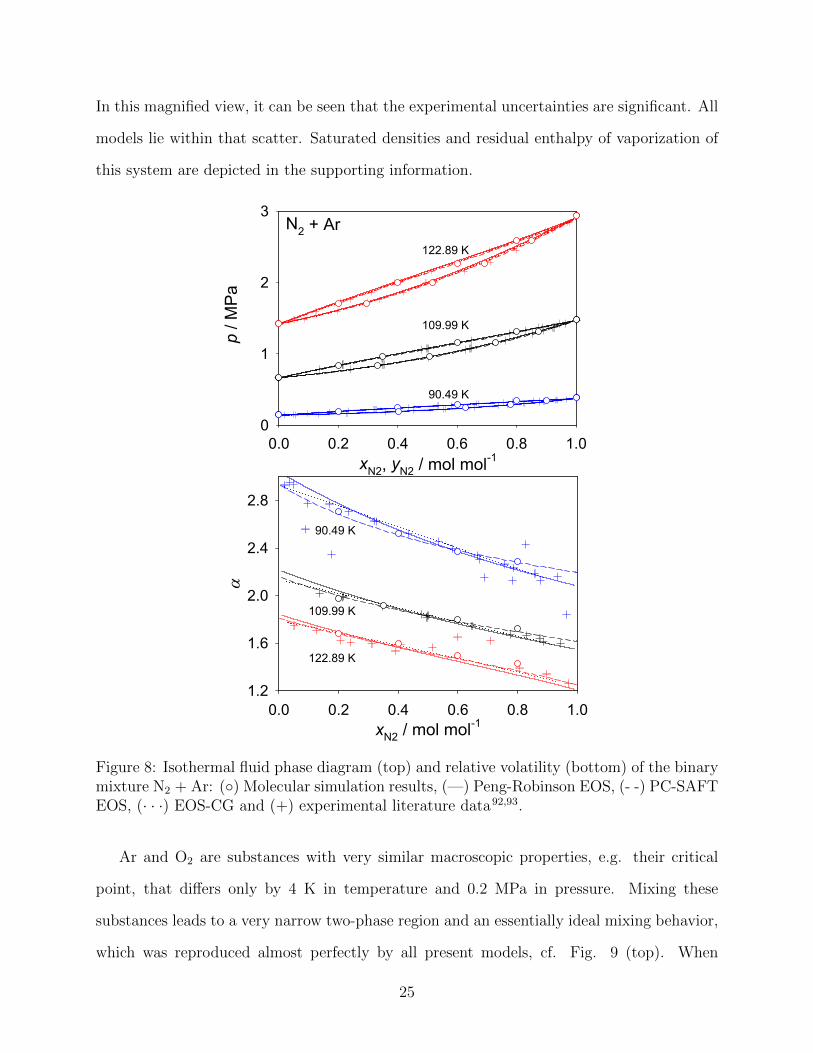
In this magnified view, it can be seen that the experimental uncertainties are significant. All

models lie within that scatter. Saturated densities and residual enthalpy of vaporization of

this system are depicted in the supporting information.

�������������

�

� �� �� � �� �

�

��

�

��

���

���

������

������

������������

�

� �� �� � �� �

�������

�

�

�������

������

������

�������

������

������

Figure 8: Isothermal fluid phase diagram (top) and relative volatility (bottom) of the binarymixture N2 + Ar: (◦) Molecular simulation results, (—) Peng-Robinson EOS, (- -) PC-SAFTEOS, (· · ·) EOS-CG and (+) experimental literature data92,93.

Ar and O2 are substances with very similar macroscopic properties, e.g. their critical

point, that differs only by 4 K in temperature and 0.2 MPa in pressure. Mixing these

substances leads to a very narrow two-phase region and an essentially ideal mixing behavior,

which was reproduced almost perfectly by all present models, cf. Fig. 9 (top). When

25

compared to the EOS-CG, MAPE values of 0.2 % for the Peng-Robinson EOS, 0.2 % for

the PC-SAFT EOS and 0.9 % for molecular simulation data were achieved for the vapor

pressure. All considered EOS show a similar behavior with respect to the relative volatility,

cf. Fig. 9 (bottom), and deviate from experimental data only at the lowest isotherm,

whereas molecular simulation data show some deviation. Due to the similarity of the two

components, the saturated mixture densities are almost constant over the whole composition

range, cf. Fig. 10 (top). Both molecular based models, i.e. atomistic simulations and the

PC-SAFT EOS, predict this behavior equally well, whereas the Peng-Robinson EOS deviates

by a constant offset of 5 mol/l in terms of the saturated liquid density. Some discrepancies

between all models were observed for the residual enthalpy of vaporization, which is shown

in Fig. 10 (bottom). For this property, the EOS-CG shows a somewhat more convex shape

than molecular simulation, the PC-SAFT and the Peng-Robinson EOS.

Binary VLE data for the mixtures H2 + O2, O2 + H2O and Ar + H2O are not presented

due to the lack of sufficient high quality experimental data. The aqueous systems were,

however, investigated on the basis of Henry’s law constant.

3.2 Binary homogeneous pvT data

Beyond VLE properties, there is also interest in homogeneous pvT data, which are discussed

for binary mixtures in this section. An equimolar composition was chosen because a maximal

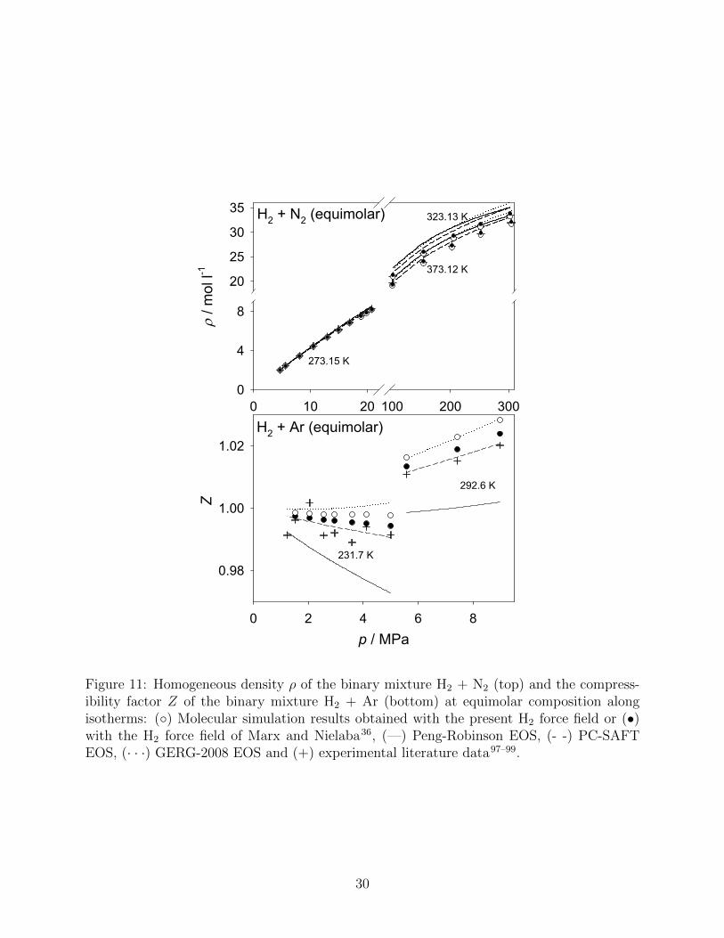
occurence of unlike molecular interactions was targeted. Fig. 11 presents the homogeneous

density for H2 + N2 (top) and the compressibility factor Z for H2 + Ar (bottom), both

properties were evaluated at given pressure and composition along isotherms. Z was chosen

for the latter mixture, because the considered experimental data are dominated by ideal

gas behavior. Unfortunately, no experimental data at higher densities were available in the

vicinity of equimolar composition. In contrast to the saturated densities of the systems

containing H2 as discussed e.g. in Fig. 2, the GERG-2008 EOS is applicable under these

conditions. Therefore, a better assessment of the models with respect to the density is

26

�������������

�

� �� � �� �� �

�

�

��

�

��

�������

������

������������

�� �� � �� �� �

�������

�

��

�

����

����

�����

�����

����

����

Figure 9: Isothermal fluid phase diagram (top) and relative volatility (bottom) of the binarymixture Ar + O2: (◦) Molecular simulation results, (—) Peng-Robinson EOS, (- -) PC-SAFTEOS, (· · ·) EOS-CG and (+) experimental literature data94–96.

27

������������

���

��

��

�

����

� ��

����

�������� ���������

��� ��� ��� ��� ��� ��

��������������

��

�

���

�� ����

��� ��

�������

���

����

��� ��

�������

�������

Figure 10: Isothermal saturated densities ρsat (top) and residual enthalpy of vaporizationhresvap (bottom) of the binary mixture Ar + O2: (◦) Molecular simulation results, (—) Peng-Robinson EOS, (- -) PC-SAFT EOS and (· · ·) EOS-CG.

28

feasible.

For H2 + N2, a large pressure and density range was covered by experimental studies,

cf. Fig. 11 (top). Both the horizontal and the vertical axes have a scale break, showing a

supercritical ”gas-like” isotherm at T = 273.15 K and supercritical ”liquid-like” isotherms

at T = 323.13 K and 373.12 K. All models perform very well at T = 273.15 K and exhibit

MAPE of ≤ 1 %. For elevated pressure and density, however, the discrepancies become

larger. This applies in particular to all EOS, which tend to overestimate the density. The

atomistic molecular simulations, both with the present (MAPE 0.7 %) and the H2 force field

from the literature36 (MAPE 0.9 %) perform very well.

The experimental data base for the mixture H2 + Ar is smaller, measurements are avail-

able up to pressures of 9 MPa, cf. Fig. 11 (bottom). Over the whole pressure range,

the atomistic molecular simulations, the PC-SAFT and the GERG-2008 EOS perform well,

whereas the Peng-Robinson EOS deviates qualitatively. Accordingly, MAPE of 0.3 %, 1.0

%, 0.5 %, 0.4 % and 0.7 % were found for the PC-SAFT EOS, the Peng-Robinson EOS,

molecular simulation with the present force field, molecular simulation with the literature

force field and the GERG-2008 EOS at T = 231.7 K, respectively.

The homogeneous pvT behavior of three binary mixtures without H2, i.e. N2 + O2, N2 +

Ar and Ar + O2, is illustrated in Fig. 12. Experimental data and the EOS-CG were used to

assess the quality of the molecular simulation data, the PC-SAFT and the Peng-Robinson

EOS.

For the system N2 + O2, cf. Fig. 12 (top), two isotherms at intermediate pressures are

presented. At 293.15 K and low density, hardly any difference between the employed models

and the experimental data can be observed. Peng-Robinson EOS, PC-SAFT EOS, EOS-

CG and molecular simulation have MAPE of 1.1 %, 0.5 %, 0.1 % and 0.3 %, respectively.

The isotherm at T = 142.25 K is below the critical temperature of O2 (Tc,O2 = 154.6 K),

therefore, a VLE of the mixture is conceivable. Consequently, the EOS-CG predicts the

critical point of N2 + O2 at p = 4.44 MPa and xN2 = 0.454 mol·mol−1 at this temperature.

29

� �� �� ��� ��� ���

��������

�

�

�

��

�

��

� ������

������������

��������

����� ��

��������

�������

� � � � �

�

����

����

����

����� ������������

�������

�������

Figure 11: Homogeneous density ρ of the binary mixture H2 + N2 (top) and the compress-ibility factor Z of the binary mixture H2 + Ar (bottom) at equimolar composition alongisotherms: (◦) Molecular simulation results obtained with the present H2 force field or (•)with the H2 force field of Marx and Nielaba36, (—) Peng-Robinson EOS, (- -) PC-SAFTEOS, (· · ·) GERG-2008 EOS and (+) experimental literature data97–99.

30

The shape of this isotherm can therefore be explained by a close passing of the critical line

of this mixture, starting from a ”gas-like” state and ending in a ”liquid-like” state. It can be

seen that the EOS-CG shows the best agreement with the experimental data. Close to the

mixtures’ critical line, molecular simulation data show the largest deviations, which may be

caused by finite size effects. State points that are not in the vicinity of the critical line agree

satisfactorily with the experimental data. The PC-SAFT and Peng-Robinson EOS agree

well with each other, but fail to reproduce the reference data in the ”liquid-like” region.

Fig. 12 (center) shows three isotherms for N2 + Ar. The results are comparable and

indicate a tendency that has been observed before. Namely, a good agreement to the refer-

ence data at low density was achieved by all employed models, whereas deviations become

increasingly severe for the Peng-Robinson EOS and, to a limited extent, also for the PC-

SAFT EOS at higher density. Results from molecular simulation agree excellently with both

the experimental data and the EOS-CG, exhibiting a MAPE value of 0.4 %. For Ar + O2

only one isotherm at low densities could be examined, which was done here in terms of the

compressibility factor, cf. Fig. 12 (bottom). The best agreement to both experimental data

and the EOS-CG was found for the molecular simulation data, whereas the Peng-Robinson

and PC-SAFT EOS deviate more or less thoroughly.

3.3 Henry’s law constant

Henry’s law constant data were used in the present work to assess aqueous systems, i.e. H2,

N2, O2 or Ar in H2O. This property is typically employed in cases where a solute is only

little soluble in a solvent. Various definitions of the Henry’s law constant are established

in the literature. The present work considers the purely temperature dependent Henry’s

law constant, which requires that the solvent is in its saturated liquid state. Consequently,

Henry’s law constant data are presented from the triple point temperature to the critical

temperature of H2O. In order to validate the results of the present work, both experimental

data and the official IAPWS correlation104,105 of these data were used.

31

��� ��� ��� ���

��������

�

�

��

��

�����

�����������

��������

��������

� �� �� �� �� ��

��������

�

��

��

��

����������������

��������

��������

�������

�������

� � � �� ��

�

����

����

���

���� �����������������

�� ����

Figure 12: Homogeneous density ρ of the binary mixtures N2 + O2 (top), N2 + Ar (center)and the compressibility factor Z of the binary mixture Ar+O2 (bottom) at equimolar com-position along isotherms: (◦) Molecular simulation results, (—) Peng-Robinson EOS, (- -)PC-SAFT EOS, (· · ·) EOS-CG and (+) experimental literature data100–103.

32

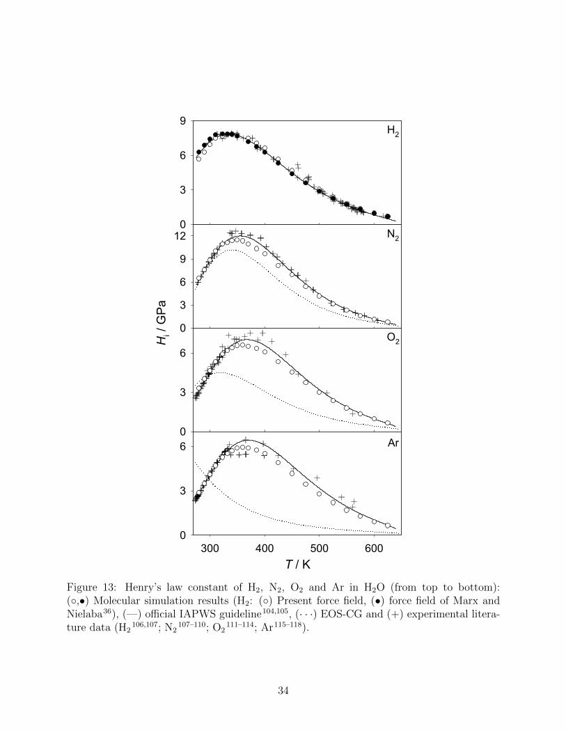
All considered aqueous systems exhibit a qualitatively similar, strongly non-monotonic

behavior, cf. Fig. 13. A pronounced maximum of the Henry’s law constant is passed

between 330 and 370 K. Note that large values of the Henry’s law constant correspond

to a low solubility, therefore, the solubility decreases with increasing temperature, passes

through a minimum and then increases again. However, quantitative differences between

the solutes are present. Close to the triple point temperature, H2 and N2 are almost equally

soluble in H2O (HH2 ≈ HN2 ≈ 6 GPa), but roughly three times less soluble than O2 and

Ar (HO2 ≈ HAr ≈ 2 GPa). Furthermore, the maximum values of the Henry’s law constant

differ significantly.

The results from molecular simulation are satisfactory, the region of increasing Henry’s

law constant at low temperature was reproduced almost perfectly for all four solutes, whereas

deviations are present at intermediate temperatures for N2, O2 and Ar. For H2, the agreement

to the reference data is satisfying throughout for both employed force fields. Nonetheless, a

disadvantage of the present force field for H2 becomes apparent here. In order to compensate

the missing electrostatic interactions of H2, which are obviously very important when H2O

is involved, the unlike LJ interaction energy had to be increased. This fact is reflected by a

rather unphysically large value of ξ = 1.52.

The EOS-CG fails to reproduce the solubility data for Ar even qualitatively and predicts

a monotonically decreasing Henry’s law constant for increasing temperature. For N2 and O2,

that behavior is predicted in a qualitatively correct way, but deviates quantitatively from

the IAPWS reference. An application of the Henry’s law constant to the fitting algorithms

for empirical Helmholtz energy EOS should therefore be considered in the future.

3.4 Ternary vapor-liquid equilibria

For higher order mixtures smaller experimental data bases can be found in the literature.

Consequently, only for two of the ten possible ternary systems experimental VLE data are

available for comparison, i.e. N2 + O2 + Ar and H2 + N2 + Ar. Since all models ap-

33

�

�

�

�

�

�

�

�

��

�

�

�

��

�

�

�����

��� �� ��� ���

��������

�

�

� ��

Figure 13: Henry’s law constant of H2, N2, O2 and Ar in H2O (from top to bottom):(◦,•) Molecular simulation results (H2: (◦) Present force field, (•) force field of Marx andNielaba36), (—) official IAPWS guideline104,105, (· · ·) EOS-CG and (+) experimental litera-ture data (H2

106,107; N2107–110; O2

111–114; Ar115–118).

34

plied in this study are based on pairwise additivity and neglect higher order interactions,

the presented results are considered as predictive. This also applies to the EOS-CG and the

GERG-2008 EOS, therefore, mainly experimental data were used as a reference for higher or-

der mixtures. The following ternary VLE diagrams show the saturated mixture compositions

at constant temperature and pressure.

Fig. 14 depicts the VLE for N2 + O2 + Ar (dry air) which was already examined in

molecular simulation studies of our group13,14. This system is characterized by a comparably

narrow two-phase region. At T = 83.6 K and pressures of about p = 0.13 MPa, cf. Fig.

14, the experimental data seem to scatter considerably, but this is rather caused by their

small temperature and pressure variations. Molecular simulations were specified to reproduce

the experimental data on the saturated liquid line and therefore seemingly scatter as well.

Nonetheless, the agreement of all employed models is satisfactory. Especially the PC-SAFT

EOS and the EOS-CG agree quite well.

A VLE phase diagram of H2 + N2 + Ar is presented in Fig. 15. This system exhibits

a large two-phase region due to the presence of H2. An excellent agreement between the

molecular simulation data, the PC-SAFT EOS and the experimental data on the saturated

liquid and vapor line was observed. The GERG-2008 EOS predicts the saturated vapor line

satisfactorily, but deviates from the experiments when the saturated liquid line is considered,

whereas the Peng-Robinson EOS predicts a two-phase region that is slightly too narrow.

Additional ternary VLE data for both of these mixtures can be found in the supporting

information.

3.5 Higher order homogeneous pvT data

Although any higher order mixture could be targeted with the considered modeling ap-

proaches, the present study is limited by experimental data availability. Therefore, homo-

geneous pvT data are only presented for one ternary and one quaternary system, i.e. N2 +

O2 + Ar (dry air) and N2 + O2 + Ar + H2O (humid air), respectively. For both mixtures,

35

��� ��� ��� ��� ��� ���

���

���

���

���

���

������

���

���

���

���

���

���� ������

������������

���������

����������������

� ����� �������������� �

�� ���

�� ���

������ ��

������������������

��

Figure 14: Fluid phase diagram of the ternary system N2 + O2 + Ar at 83 to 84 K and 0.122to 0.142 MPa: (◦) Molecular simulation results, (—) Peng-Robinson EOS, (- -) PC-SAFTEOS, (· · ·) EOS-CG and (+) experimental literature data119.

36

������������������

��� ��� �� ��� ��� ��

��� ���

�� ���

������

���

���

��

���

���

��

� ����� ������������

���

���

��

���

���

��

��������������

��������������

����

����������� �

Figure 15: Fluid phase diagram of the ternary system H2 + N2 + Ar at 100 K and 3.01 to3.05 MPa: (◦) Molecular simulation results, (—) Peng-Robinson EOS, (- -) PC-SAFT EOS,(· · ·) GERG-2008 EOS and (+) experimental literature data75.

37

large temperature and pressure ranges were studied.

The homogeneous pvT behavior along four isotherms for N2 + O2 + Ar is shown in Fig.

16. Experimental data are available at T ≤ 873.19 K and p ≤ 70 MPa. In this case, a high

quality Helmholtz energy explict EOS for standard dry air by Lemmon et al.120 was used as a

reference. The experimental data were predicted well by molecular simulation, the EOS-CG

and the PC-SAFT EOS with MAPE of 0.6 %, 0.2 % and 1.1 %, respectively. At T = 70

K, where dry air is in its liquid state, the Peng-Robinson EOS shows large deviations. It

can be seen that the EOS-CG and the molecular simulation data agree well to the dry air

EOS by Lemmon et al.120 for pressures above 70 MPa in the gaseous phase, whereas the

Peng-Robinson and the PC-SAFT EOS deviate more or less thoroughly. In the liquid state,

molecular simulation data and the PC-SAFT EOS overestimate the density on average by

0.6 % and 1.8 % (MAPE), respectively.

�������

� ��� ��� ��

�������� �

�

��

��

�

������

������

�������

����

�������

������

���������������

������������

����������

Figure 16: Homogeneous density ρ of the ternary mixture N2 + O2 + Ar at a compositionwhich represents dry air along four isotherms: (◦) Molecular simulation results, (—) Peng-Robinson EOS, (- -) PC-SAFT EOS, (· · ·) EOS-CG, (-·-) dry air EOS by Lemmon et al.120

and (+) experimental literature data121–123.

Two different compositions are discussed for the quaternary system N2 + O2 + Ar +

H2O, the first corresponding to humid air, cf. Fig. 17 (top), and the second corresponding

38

to supercritical H2O containing a substantial amount of solved gases, cf. Fig. 17 (bottom).

Since no adjustment of the PC-SAFT and the Peng-Robsinon EOS could be carried out

for the subsystems O2 + H2O and Ar + H2O due to the lack of experimental data, their

binary interaction parameter was set to kij = 0 for these calculations. Although plenty of

experimental measurements were conducted for humid air, only one experimental data point

is shown here due to varying temperatures and compositions in the experiment series. Over

the whole range of temperature and pressure, the agreement between the EOS-CG and the

present molecular simulations is excellent, a MAPE of 0.8 % was found. The PC-SAFT and

the Peng-Robinson EOS differ more or less strongly from the EOS-CG and yield MAPE of

1.5 % and 5.4 %, respectively. Fig. 17 (bottom) shows a ”water-like” composition of the four

discussed substances. It is interesting that the EOS-CG reproduces the experimental data

very well at lower pressures, whereas molecular simulation is superior at higher pressures.

One cause for the deviation of the molecular simulation results at lower pressures could be

the close proximity to the critical point of this mixture, i.e. water as the main component has

critical properties of Tc = 647.1 K, pc = 22 MPa and ρc = 17.87 mol/l. The best agreement

for this mixture was found for the PC-SAFT EOS, whereas the Peng-Robinson EOS deviates

strongly from the experimental data at high pressures.

4 Conclusion

Several models were applied to describe the mixture behavior of five substances that are

relevant for hydrogen technology. In a first step, available pure component force fields

were complemented by a new force field for H2 and subsequently adjusted to reproduce

the fluid phase behavior of all involved binary mixtures. This was done by fitting a single

temperature independent parameter to experimental vapor pressure data of binary mixtures

or, in the case of the aqueous systems, to one experimental Henry’s law constant data

point. The primary focus was on molecular simulation, however, also a molecular based

39

�� �� ��� ��� ���

��������

�

��

��

�� �����

����������

�

��������

��������

�����

������

�������

�� ��� ��� ��� ��� ���

��������

��

��

��

��������

���������������

�����������

����������������

�� ��������

���������������

�����������

����������������

�� ��������

Figure 17: Homogeneous density ρ of the quaternary mixture N2 + O2 + Ar + H2O alongfour isotherms at a composition which represents humid air (top) and supercritical H2Ocontaining ≈ 0.2 mol·mol−1 of air components (bottom): (◦) Molecular simulation results,(—) Peng-Robinson EOS, (- -) PC-SAFT EOS, (···) EOS-CG and (+) experimental literaturedata124,125.

40

EOS (PC-SAFT EOS) and empirical EOS of different complexity (Peng-Robinson EOS,

GERG-2008 EOS and EOS-CG) were studied. In addition to VLE properties, i.e. vapor

pressure, saturated densities and residual enthalpy of vaporization, also the pvT behavior

and solubility were considered. Furthermore, the thermodynamic properties of higher order

mixtures were predicted assuming pairwise additivity throughout.

Not all of the employed models could be used for every system or thermodynamic prop-

erty under the constraints of this study (one temperature independent parameter to describe

a given binary mixture pair). The Henry’s law constant of aqueous systems, e.g., is satisfac-

torily represented only by molecular simulation, whereas the cryogenic VLE of H2 mixtures

could not be calculated with the GERG-2008 EOS. In this regard, it would be desirable

that H2 mixtures receive more attention in empirical multiparameter EOS development. As

expected, results from the Peng-Robinson EOS for the saturated liquid density deviate con-

siderably. In summary, molecular modeling and simulation yields the best overall agreement

with experimental data and, at the same time, is most versatile with respect to different

thermodynamic properties and state points.

With the present molecular mixture model, a contribution to improving the availability of

thermodynamic data for the upcoming hydrogen age was made. In principle, this model can

be used to predict thermodynamic properties of this quinary mixture and its 25 subsystems

due to pairwise additivity.

Acknowledgments

The authors gratefully acknowledge the Paderborn Center for Parallel Computing (PC2) for

the generous allocation of computer time on the OCuLUS cluster and computational support

by the High Performance Computing Center Stuttgart (HLRS) under the grant MMHBF2.

The authors wish to thank Denis Saric for helping with the molecular simulations and Dr.-

Ing. Christoph Held for his assistance during the PC-SAFT EOS calculations. The present

41

research was conducted under the auspices of the Boltzmann-Zuse Society of Computational

Molecular Engineering (BZS).

Supporting Information

Supporting Information Available:

• Predictive mixture data for H2 + O2.

• Additional VLE data.

• VLE results for H2 mixtures from the GERG-2008 EOS.

• Results from the PC-SAFT and the Peng-Robinson EOS for the Henry’s law constant.

• Numerical molecular simulation data.

42

References

(1) United Nations Framework Convention on Climate Change, The Paris Agree-

ment . 2015; http://unfccc.int/files/essential_background/convention/

application/pdf/english_paris_agreement.pdf (accessed July 7, 2017).

(2) Klare, M. Resource Wars: The New Landscape of Global Conflict ; Henry Holt and

Company, New York, 2002.

(3) Bannon, I.; Collier, P. Natural Resources and Violent Conflict: Options and Actions ;

World Bank Publications, Washington, 2003.

(4) Bertuccioli, L.; Chan, A.; Hart, D.; Lehner, F.; Madden, B.; Standen, E. Study on de-

velopment of water electrolysis in the EU . 2014; Final report in fuel cells and hydrogen

joint undertaking.

(5) Edwards, P. P.; Kuznetsov, V. L.; David, W. I. F.; Brandon, N. P. Hydrogen and fuel

cells: towards a sustainable energy future. Energy Pol. 2008, 36, 4356–4362.

(6) Momirlan, M.; Veziroglu, T. N. The properties of hydrogen as fuel tomorrow in sustain-

able energy system for a cleaner planet. Int. J. Hydrogen Energy 2005, 30, 795–802.

(7) Center for Transportation and the Environment, International Fuel Cell

Bus Workshop Report . 2016; http://www.cte.tv/wp-content/uploads/2016/12/

FCBW-Report.pdf (accessed July 7, 2017).

(8) Alstom Holding, Alstom’s hydrogen train Coradia iLint first successful

run at 80 km/h. 2017; http://www.alstom.com/press-centre/2017/03/

alstoms-hydrogen-train-coradia-ilint-first-successful-run-at-80-kmh

(accessed July 7, 2017).

(9) Dunn, S. Hydrogen futures: toward a sustainable energy system. Int. J. Hydrogen

Energy 2002, 27, 235–264.

43

(10) Gotz, M.; Lefebvre, J.; Mors, F.; Koch, A. M.; Graf, F.; Bajohr, S.; Reimert, R.;

Kolb, T. Renewable Power-to-Gas: A technological and economic review. Renew. En-

ergy 2016, 85, 1371–1390.

(11) Stoll, J.; Vrabec, J.; Hasse, H. Vapor–liquid equilibria of mixtures containing nitrogen,

oxygen, carbon dioxide, and ethane. AIChE J. 2003, 49, 2187–2198.

(12) Vrabec, J.; Stoll, J.; Hasse, H. Molecular models of unlike interactions in fluid mixtures.

Mol. Sim. 2005, 31, 215–221.

(13) Huang, Y.-L.; Vrabec, J.; Hasse, H. Prediction of ternary vapor–liquid equilibria for

33 systems by molecular simulation. Fluid Phase Equilib. 2009, 287, 62–69.

(14) Eckl, B.; Schnabel, T.; Vrabec, J.; Wendland, M.; Hasse, H. Thermophysical properties

of dry and humid air by molecular simulation including dew point calculations with

the Mollier ensemble. Ind. Eng. Chem. Res. 2009, 48, 10110–10119.

(15) Vrabec, J.; Kedia, G. K.; Buchhauser, U.; Meyer-Pittroff, R.; Hasse, H. Thermody-

namic models for vapor–liquid equilibria of nitrogen+ oxygen+ carbon dioxide at low

temperatures. Cryogenics 2009, 49, 72–79.

(16) Tenorio, M.-J.; Parrott, A. J.; Calladine, J. A.; Sanchez-Vicente, Y.; Cresswell, A. J.;

Graham, R. S.; Drage, T. C.; Poliakoff, M.; Ke, J.; George, M. W. Measurement of

the vapour–liquid equilibrium of binary and ternary mixtures of CO2, N2 and H2,

systems which are of relevance to CCS technology. Int. J. Greenh. Gas Control 2015,

41, 68–81.

(17) Cresswell, A. J.; Wheatley, R. J.; Wilkinson, R. D.; Graham, R. S. Molecular simula-

tion of the thermophysical properties and phase behaviour of impure CO2 relevant to

CCS. Farad. Discuss. 2016, 192, 415–436.

44

(18) Diamantonis, N. I.; Economou, I. G. Evaluation of statistical associating fluid theory

(SAFT) and perturbed chain-SAFT equations of state for the calculation of thermo-

dynamic derivative properties of fluids related to carbon capture and sequestration.

Energy Fuels 2011, 25, 3334–3343.

(19) Diamantonis, N. I.; Boulougouris, G. C.; Mansoor, E.; Tsangaris, D. M.;

Economou, I. G. Evaluation of cubic, SAFT, and PC-SAFT equations of state for

the vapor–liquid equilibrium modeling of CO2 mixtures with other gases. Ind. Eng.

Chem. Res. 2013, 52, 3933–3942.

(20) Sun, R.; Lai, S.; Dubessy, J. Calculations of vapor–liquid equilibria of the H2O-N2

and H2O-H2 systems with improved SAFT-LJ EOS. Fluid Phase Equilib. 2015, 390,

23–33.

(21) Kunz, O.; Wagner, W. The GERG-2008 wide-range equation of state for natural

gases and other mixtures: an expansion of GERG-2004. J. Chem. Eng. Data 2012,

57, 3032–3091.

(22) Gernert, J.; Span, R. EOS–CG: A Helmholtz energy mixture model for humid gases

and CCS mixtures. J. Chem. Thermodyn. 2016, 93, 274–293.

(23) Allen, M. P.; Tildesley, D. J. Computer simulation of liquids ; Oxford University Press,

Oxford, 1989.

(24) Vrabec, J.; Stoll, J.; Hasse, H. A set of molecular models for symmetric quadrupolar

fluids. J. Phys. Chem. B 2001, 105, 12126–12133.

(25) Windmann, T.; Linnemann, M.; Vrabec, J. Fluid Phase Behavior of Nitrogen + Ace-

tone and Oxygen + Acetone by Molecular Simulation, Experiment and the Peng–

Robinson Equation of State. J. Chem. Eng. Data 2013, 59, 28–38.

45

(26) Elts, E.; Windmann, T.; Staak, D.; Vrabec, J. Fluid phase behavior from molecular

simulation: Hydrazine, Monomethylhydrazine, Dimethylhydrazine and binary mix-

tures containing these compounds. Fluid Phase Equilib. 2012, 322, 79–91.

(27) Huang, Y.-L.; Miroshnichenko, S.; Hasse, H.; Vrabec, J. Henry’s law constant from

molecular simulation: a systematic study of 95 systems. Int. J. Thermophys. 2009,

30, 1791–1810.

(28) Vrabec, J.; Huang, Y.-L.; Hasse, H. Molecular models for 267 binary mixtures vali-

dated by vapor–liquid equilibria: A systematic approach. Fluid Phase Equilib. 2009,

279, 120–135.

(29) Abascal, J. L. F.; Vega, C. A general purpose model for the condensed phases of water:

TIP4P/2005. J. Chem. Phys. 2005, 123, 234505.

(30) Vega, C.; Abascal, J. L. F. Simulating water with rigid non-polarizable models: a

general perspective. Phys. Chem. Chem. Phys. 2011, 13, 19663–19688.

(31) Shvab, I.; Sadus, R. J. Atomistic water models: Aqueous thermodynamic properties

from ambient to supercritical conditions. Fluid Phase Equilib. 2016, 407, 7–30.

(32) Koster, A.; Spura, T.; Rutkai, G.; Kessler, J.; Wiebeler, H.; Vrabec, J.; Kuhne, T. D.

Assessing the accuracy of improved force-matched water models derived from Ab initio

molecular dynamics simulations. J. Comput. Chem. 2016, 37, 1828–1838.

(33) Nagashima, H.; Tsuda, S.; Tsuboi, N.; Koshi, M.; Hayashi, K.; Tokumasu, T. An

analysis of quantum effects on the thermodynamic properties of cryogenic hydrogen

using the path integral method. J. Chem. Phys. 2014, 140, 134506.

(34) Leachman, J. W.; Jacobsen, R. T.; Penoncello, S. G.; Lemmon, E. W. Fundamental

equations of state for parahydrogen, normal hydrogen, and orthohydrogen. J. Phys.

Chem. Ref. Data 2009, 38, 721–748.

46

(35) Hirschfelder, J.; Curtiss, C. F.; Bird, R. B. Molecular theory of gases and liquids ; John

Wiley & Sons, New York, 1964.

(36) Marx, D.; Nielaba, P. Path-integral Monte Carlo techniques for rotational motion in

two dimensions: Quenched, annealed, and no-spin quantum-statistical averages. Phys.

Rev. A 1992, 45, 8968–8971.

(37) Buch, V. Path integral simulations of mixed para-D2 and ortho-D2 clusters: The

orientational effects. J. Chem. Phys. 1994, 100, 7610–7629.

(38) Darkrim, F.; Levesque, D. Monte Carlo simulations of hydrogen adsorption in single-

walled carbon nanotubes. J. Chem. Phys. 1998, 109, 4981–4984.

(39) Belof, J. L.; Stern, A. C.; Space, B. An accurate and transferable intermolecular di-

atomic hydrogen potential for condensed phase simulation. J. Chem. Theory Comput.

2008, 4, 1332–1337.

(40) Engin, C.; Vrabec, J.; Hasse, H. On the difference between a point multipole and

an equivalent linear arrangement of point charges in force field models for vapour–

liquid equilibria; partial charge based models for 59 real fluids. Mol. Phys. 2011, 109,

1975–1982.

(41) Schnabel, T.; Vrabec, J.; Hasse, H. Unlike Lennard–Jones parameters for vapor–liquid

equilibria. J. Mol. Liq. 2007, 135, 170–178.

(42) Frenkel, D.; Smit, B. Understanding Molecular Simulation: From Algorithms to Ap-

plications ; Academic Press, San Diego, 2002.

(43) Deublein, S.; Eckl, B.; Stoll, J.; Lishchuk, S. V.; Guevara-Carrion, G.; Glass, C. W.;

Merker, T.; Bernreuther, M.; Hasse, H.; Vrabec, J. ms2: A molecular simulation tool

for thermodynamic properties. Comput. Phys. Commun. 2011, 182, 2350–2367.

47

(44) Glass, C. W.; Reiser, S.; Rutkai, G.; Deublein, S.; Koster, A.; Guevara-Carrion, G.;

Wafai, A.; Horsch, M.; Bernreuther, M.; Windmann, T.; Hasse, H.; Vrabec, J. ms2: A

molecular simulation tool for thermodynamic properties, new version release. Comput.

Phys. Commun. 2014, 185, 3302–3306.

(45) Rutkai, G.; Koster, A.; Guevara-Carrion, G.; Janzen, T.; Schappals, M.; Glass, C. W.;

Bernreuther, M.; Wafai, A.; Stephan, S.; Kohns, M.; Reiser, S.; Deublein, S.;

Horsch, M.; Hasse, H.; Vrabec, J. ms2: A molecular simulation tool for thermo-

dynamic properties, release 3.0. Comput. Phys. Commun. 2017, 221, 343–351.

(46) Lustig, R. Angle-average for the powers of the distance between two separated vectors.

Mol. Phys. 1988, 65, 175–179.

(47) Flyvbjerg, H.; Petersen, H. G. Error estimates on averages of correlated data. J. Chem.

Phys. 1989, 91, 461–466.

(48) Vrabec, J.; Hasse, H. Grand Equilibrium: vapour-liquid equilibria by a new molecular

simulation method. Mol. Phys. 2002, 100, 3375–3383.

(49) Widom, B. Some topics in the theory of fluids. J. Chem. Phys. 1963, 39, 2808–2812.

(50) Shing, K. S.; Gubbins, K. E.; Lucas, K. Henry constants in non-ideal fluid mixtures:

computer simulation and theory. Mol. Phys. 1988, 65, 1235–1252.

(51) Gross, J.; Sadowski, G. Perturbed-chain SAFT: An equation of state based on a

perturbation theory for chain molecules. Ind. Eng. Chem. Res. 2001, 40, 1244–1260.

(52) Gross, J.; Sadowski, G. Application of the perturbed-chain SAFT equation of state to

associating systems. Ind. Eng. Chem. Res. 2002, 41, 5510–5515.

(53) Gross, J.; Vrabec, J. An equation-of-state contribution for polar components: Dipolar

molecules. AIChE J. 2006, 52, 1194–1204.

48

(54) Gross, J. An equation-of-state contribution for polar components: Quadrupolar

molecules. AIChE J. 2005, 51, 2556–2568.

(55) Vrabec, J.; Gross, J. Vapor- liquid equilibria simulation and an equation of state

contribution for dipole- quadrupole interactions. J. Phys. Chem. B 2008, 112, 51–60.

(56) Kleiner, M.; Sadowski, G. Modeling of polar systems using PCP-SAFT: an approach

to account for induced-association interactions. J. Phys. Chem. C 2007, 111, 15544–

15553.

(57) Tumakaka, F.; Gross, J.; Sadowski, G. Thermodynamic modeling of complex systems

using PC-SAFT. Fluid Phase Equilib. 2005, 228, 89–98.

(58) Aasen, A.; Hammer, M.; Skaugen, G.; Jakobsen, J. P.; Wilhelmsen, Ø. Thermody-

namic models to accurately describe the PVTxy-behavior of water / carbon dioxide

mixtures. Fluid Phase Equilib. 2017, 442, 125–139.

(59) Stavrou, M.; Lampe, M.; Bardow, A.; Gross, J. Continuous molecular targeting–

computer-aided molecular design (CoMT–CAMD) for simultaneous process and sol-

vent design for CO2 capture. Ind. Eng. Chem. Res. 2014, 53, 18029–18041.

(60) Kiesow, K.; Tumakaka, F.; Sadowski, G. Experimental investigation and prediction of

oiling out during crystallization process. J. Cryst. Growth 2008, 310, 4163–4168.

(61) Vins, V.; Hruby, J. Solubility of nitrogen in one-component refrigerants: Prediction

by PC-SAFT EoS and a correlation of Henry’s law constants. Int. J. Refrig. 2011,

34, 2109–2117.

(62) Peng, D.-Y.; Robinson, D. B. A new two-constant equation of state. Ind. Eng. Chem.

Fundam. 1976, 15, 59–64.

(63) Lopez-Echeverry, J. S.; Reif-Acherman, S.; Araujo-Lopez, E. Peng-Robinson equation

of state: 40 years through cubics. Fluid Phase Equilib. 2017, 447, 39–71.

49

(64) Soave, G. Equilibrium constants from a modified Redlich-Kwong equation of state.

Chem. Eng. Sci. 1972, 27, 1197–1203.

(65) Mathias, P. M.; Copeman, T. W. Extension of the Peng-Robinson equation of state to

complex mixtures: evaluation of the various forms of the local composition concept.

Fluid Phase Equilib. 1983, 13, 91–108.

(66) Stryjek, R.; Vera, J. H. PRSV: An improved PengRobinson equation of state for pure

compounds and mixtures. Can. J. Chem. Eng. 1986, 64, 323–333.

(67) Twu, C. H.; Coon, J. E.; Cunningham, J. R. A new generalized alpha function for a

cubic equation of state Part 1. Peng-Robinson equation. Fluid Phase Equilib. 1995,

105, 49–59.

(68) Dortmund Data Base. 2015; version 7.3.0.459.

(69) Sandler, S. I. Chemical, biochemical, and engineering thermodynamics ; John Wiley &

Sons, Hoboken, 2006.

(70) Wagner, W.; Pruß, A. The IAPWS formulation 1995 for the thermodynamic properties

of ordinary water substance for general and scientific use. J. Phys. Chem. Ref. Data

2002, 31, 387–535.

(71) Span, R.; Wagner, W. A new equation of state for carbon dioxide covering the fluid

region from the triple-point temperature to 1100 K at pressures up to 800 MPa. J.

Phys. Chem. Ref. Data 1996, 25, 1509–1596.

(72) Eubanks, L. S. Vapor-Liquid equilibria in the system Hydrogen-Nitrogen-Carbon

monoxide. Ph.D. thesis, Rice University, 1957.

(73) Akers, W. W.; Eubanks, L. S. Vapor-Liquid Equilibria in the System Hydrogen-

Nitrogen-Carbon Monoxide. Adv. Cryog. Eng. 1960, 3, 275–293.

50

(74) Streett, W. B.; Calado, J. C. G. Liquid-vapour equilibrium for hydrogen + nitrogen

at temperatures from 63 to 110 K and pressures to 57 MPa. J. Chem. Thermodyn.

1978, 10, 1089–1100.

(75) Xiao, J.; Liu, K. Measurement and correlation of vapor - liquid equilibrium data in

H2 - N2 - Ar system. J. Chem. Eng. (China) 1990, 8, 8–12.

(76) Span, R.; Lemmon, E. W.; Jacobsen, R. T.; Wagner, W.; Yokozeki, A. A reference

equation of state for the thermodynamic properties of nitrogen for temperatures from

63.151 to 1000 K and pressures to 2200 MPa. J. Phys. Chem. Ref. Data 2000, 29,

1361–1433.

(77) Calado, J. C. G.; Streett, W. B. Liquid-vapor equilibrium in the system H2 + Ar at

temperatures from 83 to 141 K and pressures to 52 MPa. Fluid Phase Equilib. 1979,

2, 275–282.

(78) Ostronov, M. G.; Shatskaya, L. V.; Finyagina, R. A.; Brodskaya, L. F.; Zhirnova, N. A.

Gas-Liquid Phase Equilibrium in the Argon-Hydrogen System at Intermediate Pres-

sures. Russ. J. Phys. Chem. 1977, 51, 1407–1409.

(79) Volk, H.; Halsey Jr., G. D. Solubility of hydrogen and deuterium in liquid argon. J.

Chem. Phys. 1960, 33, 1132–1139.

(80) Mullins, J. C.; Ziegler, W. T. Phase equilibria in the argon-helium and argon-hydrogen

systems from 68 to 108 K and pressures to 120 atmospheres. Adv. Cryog. Eng. 1965,

10, 171–181.

(81) DeVaney, W.; Berryman, J. M.; Kao, P.-L.; Eakin, B. High temperature VLE mea-

surements for substitute gas components . 1978; GPA Research Report RR-30.

(82) Gillespie, P. C.; Wilson, G. M. Vapor-Liquid Equilibrium Data on Water-Substitute

51

Gas Components:N2-H2O,H2-H2O,CO-H2O,H2-CO-H2O, and H2S-H2O . 1982; GPA

Research Report RR-48.

(83) Ipat’ev, V. V.; Teodorovich, V. P. Solubility of hydrogen in water under pressure at

elevated temperatures. Zhur. Obsh. Khim 1934, 4, 395–397.

(84) Kling, G.; Maurer, G. The solubility of hydrogen in water and in 2-aminoethanol

at temperatures between 323 K and 423 K and pressures up to 16 MPa. J. Chem.

Thermodyn. 1991, 23, 531–541.

(85) Maslennikova, V. Y.; Goryunova, N. P.; Subbotina, L. A.; Tsiklis, D. S. The solubility

of water in compressed hydrogen. Russ. J. Phys. Chem. 1976, 50, 240–243.

(86) Dodge, B. F. Isotherms and isobars for air separation studies. Chem. Metall. Eng.

1928, 35, 622.

(87) Baidakov, V. G.; Kaverin, A. M.; Andbaeva, V. N. The liquid-gas interface of oxygen-

nitrogen solutions: 1. Surface tension. Fluid Phase Equilib. 2008, 270, 116–120.

(88) Maslennikova, V. Y.; Vdovina, N. A.; Tsiklis, D. S. The solubility of water in com-

pressed nitrogen. Russ. J. Phys. Chem. 1971, 45, 1354.

(89) Maslennikova, V. Y. The solubility of nitrogen in water. Trudy GIAP, Moscow 1971,

12, 82–87.

(90) Saddington, A. W.; Krase, N. W. Vapor-Liquid Equilibria in the System Nitrogen-

Water. J. Am. Chem. Soc. 1934, 56, 353–361.

(91) Japas, M. L.; Franck, E. U. High Pressure Phase Equilibria and PVT-Data. of the

Water-Nitrogen System to 673 K and 250 MPa. Ber. Bunsenges. Phys. Chem. 1985,

89, 793–800.

(92) Narinskii, G. B. Liquid-vapor equilibrium in argon-nitrogen system. I. Experimental

data and their verification. Russ. J. Phys. Chem. 1966, 40, 1093–1096.

52

(93) Liu, K.; Wang, W. VLE Measurement and Correlation of N2-Ar-CH4 System at 122.89

K. J. Chem. Eng. (China) 1988, 16, 58–63.

(94) Bourbo, P.; Ischkin, I. Study of the vapor-liquid equilibrium of the system argon-

oxygen. Phys. Z. Sowjetunion 1936, 10, 271–291.

(95) Baba-Ahmed, A. Appareillage pour l’etude des equilibre liquide–vapeur dans le do-

maine cryogenique conception et developpement. Ph.D. thesis, Ecole des Mines de

Paris, 1999.

(96) Narinskii, G. B. Investigation of the liquid-vapor equilibrium in the oxygen-argon

system. Kislorod 1957, 10, 9–16.

(97) Bennett, C. O.; Dodge, B. F. Compressibilities of mixtures of hydrogen and nitrogen

above 1000 atmospheres. Ind. Eng. Chem. 1952, 44, 180–185.

(98) Verschoyle, T. T. H. Isotherms of Hydrogen, of Nitrogen, and of Hydrogen-Nitrogen

Mixtures, at 0◦ and 20◦ C., up to a Pressure of 200 Atmospheres. Proc. R. Soc. A

1926, 111, 552–576.

(99) Zandbergen, P.; Beenakker, J. J. M. Experimental determination of the volume change

on mixing for gaseous N2-H2, Ar-H2 and Ar-N2 between 170 and 292◦ K up to 100

ATM. Physica 1967, 33, 343–365.

(100) Kuenen, J. P.; Verschoyle, T.; van Urk, A. T. Isotherms of Diatomic Substances and

their Binary Mixtures. XX. The Critical Curve of Oxygen - Nitrogen Mixtures, the

Critical Phenomena and some Isotherms of Two Mixtures of 50% and 75% by Volume

of Oxygen in the Neighborhood of the Critical Region. Proc. R. Acad. 1922, 22, 49–64.

(101) Palavra, A. M. Effect of pressure and temperature on excess properties in the system

argon-nitrogen. M.Sc. thesis, Universidade Tecnica De Lisboa, 1979.

53

(102) Crain Jr, R. W.; Sonntag, R. E. Advances in Cryogenic Engineering ; Springer, New

York, 1966; pp 379–391.

(103) Masson, I.; Dolley, L. G. F. The Pressures of Gaseous Mixtures. Proc. R. Soc. A 1923,

103, 524–538.

(104) Fernandez-Prini, R.; Alvarez, J. L.; Harvey, A. H. Henry’s constants and vapor–liquid

distribution constants for gaseous solutes in H2O and D2O at high temperatures. J.

Phys. Chem. Ref. Data 2003, 32, 903–916.

(105) International Association for the Properties of Water and Steam, Guideline on the

Henry’s Constant and Vapor-Liquid Distribution Constant for Gases in H2O and D2O

at High Temperatures . 2004.

(106) Morris, D. R.; Yang, L.; Giraudeau, F.; Sun, X.; Steward, F. R. Henry’s law constant

for hydrogen in natural water and deuterium in heavy water. Phys. Chem. Chem.

Phys. 2001, 3, 1043–1046.

(107) Alvarez, J.; Fernandez-Prini, R. A semiempirical procedure to describe the thermo-

dynamics of dissolution of non-polar gases in water. Fluid Phase Equilib. 1991, 66,

309–326.

(108) Rettich, T. R.; Battino, R.; Wilhelm, E. Solubility of gases in liquids. XVI. Henry’s law

coefficients for nitrogen in water at 5 to 50◦ C. J. Solution Chem. 1984, 13, 335–348.

(109) Cosgrove, B. A.; Walkley, J. Solubilities of gases in H2O and 2H2O. J. Chromatogr. A

1981, 216, 161–167.

(110) Alvarez, J.; Crovetto, R.; Fernandez-Prini, R. The dissolution of N2 and of H2 in water

from room temperature to 640 K. Ber. Bunsenges. Phys. Chem. 1988, 92, 935–940.

54

(111) Rettich, T. R.; Battino, R.; Wilhelm, E. Solubility of gases in liquids. 22. High-

precision determination of Henry’s law constants of oxygen in liquid water from T=

274 K to T= 328 K. J. Chem. Thermodyn. 2000, 32, 1145–1156.

(112) Benson, B. B.; Krause, D.; Peterson, M. A. The solubility and isotopic fractionation

of gases in dilute aqueous solution. I. Oxygen. J. Solution Chem. 1979, 8, 655–690.

(113) Rettich, T. R.; Handa, Y. P.; Battino, R.; Wilhelm, E. Solubility of gases in liquids. 13.

High-precision determination of Henry’s constants for methane and ethane in liquid

water at 275 to 328 K. J. Phys. Chem. 1981, 85, 3230–3237.

(114) Cramer, S. D. The solubility of oxygen in brines from 0 to 300◦ C. Ind. Eng. Chem.

Process Des. Dev. 1980, 19, 300–305.

(115) Rettich, T. R.; Battino, R.; Wilhelm, E. Solubility of gases in liquids. 18. High-

precision determination of Henry fugacities for argon in liquid water at 2 to 40◦ C. J.

Solution Chem. 1992, 21, 987–1004.

(116) Krause, D.; Benson, B. B. The solubility and isotopic fractionation of gases in dilute

aqueous solution. IIa. Solubilities of the noble gases. J. Solution Chem. 1989, 18,

823–873.

(117) Potter, R. W.; Clynne, M. A. The solubility of the noble gases He, Ne, Ar, Kr, and

Xe in water up to the critical point. J. Solution Chem. 1978, 7, 837–844.

(118) Crovetto, R.; Fernandez-Prini, R.; Japas, M. L. Solubilities of inert gases and methane

in H2O and in D2O in the temperature range of 300 to 600 K. J. Chem. Phys. 1982,

76, 1077–1086.

(119) Fastovskii, V. G.; Petrovskii, Y. V. A study of the vapor-liquid equilibrium in the

system oxygen-argon-nitrogen. Zh. Fiz. Khim. 1957, 31, 836–841.

55

(120) Lemmon, E. W.; Jacobsen, R. T.; Penoncello, S. G.; Friend, D. G. Thermodynamic

properties of air and mixtures of nitrogen, argon, and oxygen from 60 to 2000 K at

pressures to 2000 MPa. J. Phys. Chem. Ref. Data. 2000, 29, 331–385.

(121) Holborn, L.; Schultze, H. Uber die Druckwage und die Isothermen von Luft, Argon

und Helium zwischen 0 und 200◦ C. Ann. Phys. 1915, 352, 1089–1111.

(122) Kozlov, A. Experimental investigation of the specific volumes of air in the 20-600◦C

temperature range and 20-700 bar pressure range. Ph.D. thesis, Moscow, 1968.

(123) Diller, D. E.; Aragon, A. S.; Laesecke, A. Measurements of the viscosity of compressed

liquid air at temperatures between 70 and 130 K. Cryogenics 1991, 31, 1070–1072.

(124) Japas, M. L.; Franck, E. U. High Pressure Phase Equilibria and PVT-Data of the

Water-Oxygen System Including Water-Air to 673 K and 250 MPa. Ber. Bunsenges.

Phys. Chem. 1985, 89, 1268–1275.

(125) Ulbig, P.; Trusler, M.; Wendland, M.; Woll, O.; Nieto de Castro, C. A. Summary

report on experimental results for thermodynamic and transport properties, AA-CAES,

Deliverable Report D4.1 . 2005.

TOC Graphic

56

Nitrogen

Hydrogen

Oxygen

Argon

Water Mol. Sim. EOS-CG

GERG-2008 PC-SAFT EOS

PR EOS

TOC Graphic

57

Supporting information for:

Molecular models for the hydrogen age:

Hydrogen, nitrogen, oxygen, argon and water

Andreas Koster,† Monika Thol,‡ and Jadran Vrabec∗,†

†Lehrstuhl fur Thermodynamik und Energietechnik, Universitat Paderborn,

33098 Paderborn, Germany

‡Lehrstuhl fur Thermodynamik, Ruhr-Universitat Bochum, 44801 Bochum, Germany

E-mail: jadran.vrabec@upb.de

Phone: +49-5251 60-2421. Fax: +49 5251 60-3522

Abstract

This supporting information contains predictive mixture data for H2 + O2, ad-

ditional VLE data for mixtures discussed in the main manuscript, VLE results for

H2 mixtures from the GERG-2008 EOS, results from the PC-SAFT and the Peng-

Robinson EOS for the Henry’s law constant and all molecular simulation data with

the associated statistical uncertainty in numerical form. The confidence level for the

reported data is 68.3 % (±1 standard deviation).

S1

Contents

1 Predictive mixture data for H2 + O2 S3

2 Additional VLE data S4

3 VLE results for H2 mixtures from the GERG-2008 EOS S8

4 Henry’s law constant from the PC-SAFT and the Peng-Robinson EOS S9

5 Numerical molecular simulation data S10

5.1 Binary mixtures . . . . . . . . . . . . . . . . . . . . . . . . . . . . . . . . . . S10

5.1.1 Hydrogen + nitrogen . . . . . . . . . . . . . . . . . . . . . . . . . . . S10

5.1.2 Hydrogen + argon . . . . . . . . . . . . . . . . . . . . . . . . . . . . S13

5.1.3 Nitrogen + oxygen . . . . . . . . . . . . . . . . . . . . . . . . . . . . S16

5.1.4 Nitrogen + argon . . . . . . . . . . . . . . . . . . . . . . . . . . . . . S18

5.1.5 Argon + oxygen . . . . . . . . . . . . . . . . . . . . . . . . . . . . . . S20

5.1.6 Nitrogen + water . . . . . . . . . . . . . . . . . . . . . . . . . . . . . S22

5.1.7 Hydrogen + water . . . . . . . . . . . . . . . . . . . . . . . . . . . . S23

5.1.8 Solubility data of aqueous systems . . . . . . . . . . . . . . . . . . . S25

5.2 Ternary mixtures . . . . . . . . . . . . . . . . . . . . . . . . . . . . . . . . . S26

5.2.1 Nitrogen + oxygen + argon . . . . . . . . . . . . . . . . . . . . . . . S26

5.2.2 Hydrogen + nitrogen + argon . . . . . . . . . . . . . . . . . . . . . . S28

5.3 Quaternary mixture . . . . . . . . . . . . . . . . . . . . . . . . . . . . . . . . S29

5.3.1 Nitrogen + oxygen + argon + water . . . . . . . . . . . . . . . . . . S29

References S31

S2

1 Predictive mixture data for H2 + O2

No experimental data were available for this mixture so that the results shown in Fig. S1

are strictly predictive (no binary interaction parameter was adjusted).

������

�����������

��� ��� �� ��� ��� ��

�������

�

�

�

�

� ������

�

Figure S1: Isothermal fluid phase diagram of the binary mixture H2 + O2: (◦, �) Molecularsimulation results obtained with the present H2 force field or (•, �) with the H2 force field ofMarx and NielabaS1, (—) Peng-Robinson EOS and (- -) PC-SAFT EOS. For comparison, (�)and (�) depict molecular simulation data with binary interaction parameters of the chemi-cally similar mixture H2 + N2, cf. Table 4 in the main manuscript. Statistical uncertaintiesof the molecular simulation data are only shown if they exceed symbol size.

S3

2 Additional VLE data

������������

�

�

��

�

��

�������� ���������

��� ��� ��� ��� ��� ��

��������������

���

��

��

���

���

����

����

������������

���

����

����������������

�������

Figure S2: Isothermal saturated densities ρsat (top) and residual enthalpy of vaporizationhresvap (bottom) of the binary mixture H2 + Ar: (◦) Molecular simulation results obtainedwith the present H2 force field or (•) with the H2 force field of Marx and NielabaS1, (—) Peng-Robinson EOS and (- -) PC-SAFT EOS. Statistical uncertainties of the molecularsimulation data are only shown if they exceed symbol size.

S4

������������

�

�

��

��

�

�������� ���������

��� ��� �� ��� ��� ��

��������������

���

��

���

��� ���

�������

�������

�������

�������

��� ���

���

�������

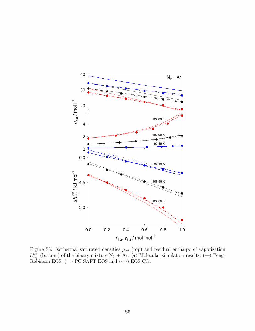
Figure S3: Isothermal saturated densities ρsat (top) and residual enthalpy of vaporizationhresvap (bottom) of the binary mixture N2 + Ar: (•) Molecular simulation results, (—) Peng-Robinson EOS, (- -) PC-SAFT EOS and (· · ·) EOS-CG.

S5

��� ��� ��� ��� ��� ���

���

���

���

���

���

������

���

���

���

���

���

���� ������

������������

�����

��������������

� ����� �������������� �

�� ���

�� ���

������ ��

� ���� �����������

��

Figure S4: Fluid phase diagram of the ternary system N2 + O2 + Ar at 120 K and 1.95 to1.99 MPa: (◦) Molecular simulation results, (—) Peng-Robinson EOS, (- -) PC-SAFT EOS,(· · ·) EOS-CG and (+) experimental literature dataS2.

S6

������������������

��� ��� �� ��� ��� ��

��� ���

�� ���

������

���

���

��

���

���

��

� ����� ������������

���

���

��

���

���

��

��������������

��������������

����

��� ����������

Figure S5: Fluid phase diagram of the ternary system H2 + N2 + Ar at 100 K and 2.04 to2.09 MPa: (◦) Molecular simulation results, (—) Peng-Robinson EOS, (- -) PC-SAFT EOS,(· · ·) GERG-2008 EOS and (+) experimental literature dataS3.

S7

3 VLE results for H2 mixtures from the GERG-2008

EOS

In Fig. S6 the GERG-2008 EOS was used to calculate the phase envelope of H2 mixtures.

It can be seen that in some cases a false liquid-liquid equilibrium is predicted (bottom). In

other cases, the vapor pressure is strongly overestimated. However, cryogenic H2 mixtures

were not the main focus during the development of the GERG-2008 EOS and its normal

range of validity in temperature is specified as 90 to 450 KS4, which means that the lowest

isotherm is an extrapolation.

�

��

��

������� ������

�����

�

�����

�� ��

����������

��

��� ��� ��� ��� ��� ���

�������

�

��

��

�����������

�����

������

Figure S6: Isothermal fluid phase diagram of the binary mixtures H2 + N2 (top) and H2 +Ar (bottom): (+) Experimental literature dataS3,S5–S11 and (· · ·) GERG-2008 EOSS4.

S8

4 Henry’s law constant from the PC-SAFT and the

Peng-Robinson EOS

As discussed in the main manuscript, both the PC-SAFT and the Peng-Robinson EOS fail to

reproduce the Henry’s law constant of H2, N2, O2 and Ar in H2O qualitatively, cf. Fig. S7. A

single temperature independent binary interaction parameter was used for these calculations,

cf. Table 4 in the main manuscript.

�

�

�

�

�

�

�

�

��

�

�

�

��

�

�

�����

��� �� ��� ���

��������

�

�

� ��

Figure S7: Henry’s law constant of H2, N2, O2 and Ar in H2O (from top to bottom): (—,black) official IAPWS guidelineS12,S13, (—, red) Peng-Robinson EOS, (- -) PC-SAFT EOS,(···) EOS-CG and (+) experimental literature data (H2

S14,S15; N2S15–S18; O2

S19–S22; ArS23–S26).

S9

5 Numerical molecular simulation data

5.1 Binary mixtures

5.1.1 Hydrogen + nitrogen

Table S1: Homogeneous density data from molecular simulation for the equimolar mixtureH2 + N2 using the present as well as the H2 force field of Marx and NielabaS1. Statisticaluncertainties are denoted by δ.

T p ρH2,present δρH2,present ρH2,Marx δρH2,Marx

K MPa mol/l mol/l mol/l mol/l273.15 4.667 2.0155 0.0002 2.0194 0.0002273.15 5.642 2.4250 0.0002 2.4309 0.0002273.15 8.082 3.4288 0.0003 3.4408 0.0003273.15 10.530 4.4053 0.0005 4.4257 0.0005273.15 12.979 5.3496 0.0006 5.3785 0.0006273.15 14.938 6.0814 0.0007 6.1189 0.0007273.15 16.897 6.7892 0.0008 6.8354 0.0008273.15 18.858 7.4760 0.0009 7.5344 0.0009273.15 19.838 7.812 0.001 7.8738 0.0008273.15 20.818 8.1423 0.0009 8.207 0.001

323.13 101.125 20.956 0.002 21.279 0.002323.13 153.849 25.587 0.002 26.009 0.002323.13 205.233 28.817 0.002 29.303 0.002323.13 252.193 31.138 0.002 31.672 0.002323.13 302.878 33.209 0.002 33.785 0.002

373.12 100.861 19.087 0.002 19.348 0.002373.12 153.755 23.735 0.002 24.096 0.002373.12 202.721 26.879 0.002 27.303 0.002373.12 252.448 29.405 0.002 29.883 0.002373.12 304.578 31.588 0.002 32.105 0.002

S10

Tab

leS2:

Vap

or-l

iquid

equilib

rium

dat

afr

omm

olec

ula

rsi

mula

tion

for

H2

+N

2usi

ng

the

pre

sent

H2

forc

efiel

d.

Sta

tist

ical

unce

rtai

nti

esar

eden

oted

byδ.

Tp

δpxH2

y H2

δyH2

ρliq

δρliq

ρvap

δρvap

∆hres

vδ∆

hres

v

KM

Pa

MP

am

ol/m

olm

ol/m

olm

ol/m

olm

ol/l

mol

/lm

ol/l

mol

/lkJ/m

olkJ/m

ol83.1

50.

196

0.00

10.

000.

000

0.00

027.8

950.

005

0.30

20.

002

5.39

90.

001

83.1

51.

327

0.00

50.

030.

816

0.00

228.0

670.

005

2.01

00.

007

5.20

80.

001

83.1

52.

090.

010.

050.

862

0.00

228.1

820.

006

3.17

0.02

5.04

60.

002

83.1

53.

280.

020.

080.

890

0.00

228.3

820.

006

5.02

0.03

4.80

30.

002

83.1

54.

010.

030.

100.

900

0.00

228.5

110.

007

6.13

0.04

4.64

90.

003

83.1

55.

060.

050.

120.

903

0.00

228.7

100.

008

7.77

0.07

4.45

00.

003

83.1

56.

590.

070.

160.

900

0.00

328.9

940.

005

10.2

0.1

4.14

70.

004

83.1

57.

90.

10.

190.

892

0.00

329.2

230.

005

12.3

0.2

3.88

0.01

83.1

510.4

0.2

0.24

0.86

30.

005

29.6

810.

008

16.1

0.3

3.38

0.01

83.1

514.1

0.4

0.33

0.83

30.

006

30.1

60.

0321.0

0.6

2.64

0.02

100

0.79

40.

003

0.00

0.00

00.

000

24.6

620.

008

1.14

60.

004

4.55

40.

002

100

1.81

80.

005

0.03

0.47

90.

002

24.7

170.

007

2.52

60.

007

4.40

20.

003

100

2.51

0.01

0.05

0.58

30.

002

24.8

00.

013.

470.

014.

268

0.00

410

03.

510.

020.

080.

661

0.00

224.8

40.

014.

820.

024.

050.

0110

04.

190.

020.

100.

687

0.00

224.9

10.

015.

780.

033.

900.

0110

05.

130.

030.

120.

699

0.00

325.0

80.

017.

160.

043.

680.

0110

06.

420.

040.

160.

708

0.00

325.2

390.

009

9.08

0.06

3.38

0.01

100

8.39

0.05

0.24

0.71

70.

003

24.6

90.

0111.8

50.

072.

730.

0110

010.2

00.

070.

330.

695

0.00

424.0

40.

0514.6

0.1

2.02

0.02

110.

31.

512

0.00

50.

000.

000

0.00

022.2

10.

012.

243

0.00

73.

813

0.00

411

0.3

2.44

0.01

0.03

0.27

90.

002

22.2

40.

013.

500.

013.

660.

0111

0.3

3.05

0.01

0.05

0.37

00.

002

22.1

30.

014.

320.

013.

510.

0111

0.3

3.89

0.01

0.08

0.45

30.

002

22.0

50.

015.

490.

023.

300.

0111

0.3

4.65

0.02

0.10

0.47

80.

003

22.2

90.

016.

690.

033.

120.

0111

0.3

5.24

0.02

0.12

0.51

70.

003

22.1

30.

027.

410.

032.

970.

0111

0.3

6.04

0.03

0.16

0.52

70.

003

21.6

10.

028.

710.

042.

610.

0111

0.3

6.82

0.03

0.19

0.52

60.

004

21.4

60.

0210.1

10.

052.

310.

02

S11

Tab

leS3:

Vap

or-l

iquid

equilib

rium

dat

afr

omm

olec

ula

rsi

mula

tion

for

H2

+N

2usi

ng

the

H2

forc

efiel

dof

Mar

xan

dN

iela

baS1.

Sta

tist

ical

unce

rtai

nti

esar

eden

oted

byδ.

Tp

δpxH2

y H2

δyH2

ρliq

δρliq

ρvap

δρvap

∆hres

vδ∆

hres

v

KM

Pa

MP

am

ol/m

olm

ol/m

olm

ol/m

olm

ol/l

mol

/lm

ol/l

mol

/lkJ/m

olkJ/m

ol83.1

50.

196

0.00

20.

000.

000

0.00

027.8

990.

005

0.30

20.

003

5.40

10.

001

83.1

51.

270.

010.

030.

812

0.00

228.1

110.

005

1.95

20.

008

5.19

40.

002

83.1

51.

980.

010.

050.

866

0.00

128.2

550.

005

3.09

80.

011

5.02

40.

002

83.1

53.

050.

010.

080.

898

0.00

128.4

610.

005

4.89

70.

018

4.76

10.

002

83.1

53.

760.

020.

100.

903

0.00

128.5

890.

007

6.15

80.

032

4.57

90.

003

83.1

54.

630.

020.

120.

910

0.00

128.7

580.

005

7.74

80.

034

4.36

40.

003

83.1

55.

960.

030.

160.

910

0.00

129.0

130.

007

10.3

120.

052

4.03

30.

004

83.1

57.

060.

040.

190.

906

0.00

129.2

110.

016

12.5

010.

071

3.76

0.01

83.1

59.

180.

070.

240.

890

0.00

229.5

950.

026

16.7

420.

120

3.26

0.01

83.1

514.8

0.3

0.40

0.81

50.

005

30.6

240.

085

25.7

700.

452

1.89

0.02

100

0.79

20.

003

0.00

0.00

00.

000

24.6

440.

008

1.14

30.

004

4.55

20.

002

100

1.81

50.

005

0.03

0.48

50.

002

24.7

600.

009

2.52

20.

007

4.40

90.

003

100

2.47

0.01

0.05

0.58

40.

002

24.8

290.

009

3.44

70.

008

4.26

10.

003

100

3.48

0.01

0.08

0.66

60.

001

24.9

130.

008

4.88

00.

014

4.02

90.

003

100

4.12

0.01

0.10

0.69

00.

002

24.9

760.

008

5.85

40.

016

3.86

30.

004

100

4.84

0.02

0.12

0.71

10.

002

24.9

990.

009

6.94

50.

023

3.67

0.01

100

5.98

0.02

0.16

0.72

80.

002

25.0

750.

011

8.71

20.

031

3.37

0.01

100

6.88

0.03

0.19

0.73

10.

002

25.0

810.

025

10.1

840.

041

3.11

0.01

100

8.44

0.04

0.24

0.70

80.

003

25.1

230.

033

13.1

190.

068

2.59

0.01

100

10.5

30.

120.

330.

579

0.00

724.9

340.

101

19.2

970.

212

1.36

0.03

110.

31.

515

0.00

40.

000.

000

0.00

022.2

070.

028

2.25

10.

006

3.80

90.

004

110.

32.

440.

010.

030.

280

0.00

122.1

890.

031

3.48

10.

009

3.66

0.01

110.

33.

030.

010.

050.

375

0.00

222.1

740.

028

4.30

00.

011

3.52

0.01

110.

33.

940.

010.

080.

455

0.00

222.1

630.

021

5.62

10.

016

3.29

0.01

110.

34.

460.

010.

100.

488

0.00

222.0

760.

022

6.37

90.

018

3.13

0.01

110.

35.

160.

020.

120.

511

0.00

222.0

480.

019

7.50

30.

023

2.91

0.01

110.

36.

060.

020.

160.

543

0.00

221.9

040.

014

8.84

70.

036

2.64

0.01

110.

36.

800.

030.

190.

536

0.00

321.7

580.

057

10.3

310.

045

2.32

0.01

110.

38.

000.

040.

240.

509

0.00

621.4

740.

042

13.1

520.

071

1.71

0.04

S12

5.1.2 Hydrogen + argon

Table S4: Homogeneous density data from molecular simulation for the equimolar mixtureH2 + Ar using the present as well as the H2 force field of Marx and NielabaS1. Statisticaluncertainties are denoted by δ.

T p ρH2,present δρH2,present ρH2,Marx δρH2,Marx

K MPa mol/l mol/l mol/l mol/l170.5 0.210 0.1484 0.0001 0.1484 0.0001170.5 0.403 0.2859 0.0001 0.2860 0.0001170.5 0.606 0.4304 0.0001 0.4307 0.0001170.5 1.016 0.7252 0.0001 0.7262 0.0001170.5 1.230 0.8798 0.0001 0.8810 0.0001

231.7 1.226 0.6372 0.0001 0.6377 0.0001231.7 1.520 0.7901 0.0001 0.7909 0.0001231.7 2.047 1.0643 0.0001 1.0658 0.0001231.7 2.564 1.3332 0.0001 1.3356 0.0001231.7 2.959 1.5388 0.0001 1.5420 0.0001231.7 3.587 1.8657 0.0002 1.8703 0.0001231.7 4.114 2.1398 0.0002 2.1460 0.0002231.7 5.005 2.6043 0.0003 2.6129 0.0003

292.6 5.583 2.2578 0.0002 2.2645 0.0002292.6 7.427 2.9849 0.0003 2.9961 0.0002292.6 8.977 3.5882 0.0004 3.6040 0.0003

S13

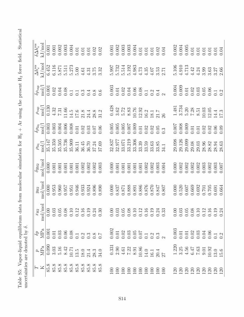
Tab

leS5:

Vap

or-l

iquid

equilib

rium

dat

afr

omm

olec

ula

rsi

mula

tion

for

H2

+A

rusi

ng

the

pre

sent

H2

forc

efiel

d.

Sta

tist

ical

unce

rtai

nti

esar

eden

oted

byδ.

Tp

δpxH2

y H2

δyH2

ρliq

δρliq

ρvap

δρvap

∆hres

vδ∆

hres

v

KM

Pa

MP

am

ol/m

olm

ol/m

olm

ol/m

olm

ol/l

mol

/lm

ol/l

mol

/lkJ/m

olkJ/m

ol85.8

0.09

00.

001

0.00

0.00

00.

000

35.1

470.

003

0.13

00.

001

6.45

20.

001

85.8

3.03

0.01

0.03

0.95

30.

001

35.3

500.

003

4.32

0.02

6.11

60.

001

85.8

5.16

0.03

0.05

0.96

00.

001

35.5

050.

004

7.31

0.04

5.87

10.

002

85.8

8.42

0.06

0.08

0.95

70.

001

35.7

360.

006

11.6

60.

085.

511

0.00

385.8

10.7

10.

080.

100.

951

0.00

135.9

090.

008

14.5

0.1

5.27

30.

004

85.8

13.5

0.1

0.12

0.94

60.

001

36.1

10.

0117.6

0.1

5.00

0.01

85.8

18.0

0.2

0.16

0.93

30.

002

36.4

50.

0221.8

0.3

4.61

0.01

85.8

21.4

0.3

0.19

0.92

40.

002

36.7

00.

0324.4

0.4

4.31

0.01

85.8

28.3

0.8

0.24

0.89

60.

002

37.2

40.

0728.8

0.8

3.75

0.02

85.8

34.0

0.7

0.30

0.89

00.

003

37.6

90.

0631.2

0.6

3.32

0.02

100

0.33

10.

002

0.00

0.00

00.

000

32.8

370.

005

0.42

80.

003

5.99

70.

001

100

2.90

0.01

0.03

0.83

70.

001

32.9

770.

005

3.62

0.01

5.73

20.

002

100

4.61

0.02

0.05

0.87

10.

001

33.0

710.

005

5.72

0.02

5.51

40.

003

100

7.22

0.03

0.08

0.88

80.

001

33.2

190.

007

8.83

0.04

5.19

20.

003

100

8.91

0.05

0.10

0.89

10.

001

33.3

060.

009

10.7

60.

064.

983

0.00

410

010.8

60.

070.

120.

886

0.00

133.3

90.

0112.9

20.

084.

730.

0110

014.0

0.1

0.16

0.87

60.

002

33.5

90.

0216.2

0.1

4.35

0.01

100

16.1

0.2

0.19

0.87

00.

002

33.6

30.

0218.1

0.2

4.07

0.01

100

20.4

0.3

0.24

0.84

70.

003

33.8

50.

0521.7

0.4

3.53

0.02

100

272

0.33

0.80

70.

004

34.1

0.3

262

2.71

0.04

120

1.22

00.

003

0.00

0.00

00.

000

29.0

980.

007

1.48

10.

004

5.10

60.

002

120

3.25

0.01

0.03

0.52

00.

002

29.1

260.

008

3.73

40.

009

4.91

00.

004

120

4.56

0.01

0.05

0.60

70.

002

29.0

990.

009

5.20

0.01

4.71

30.

005

120

6.47

0.02

0.08

0.66

90.

002

29.0

80.

017.

280.

024.

420.

0112

07.

630.

030.

100.

692

0.00

229.0

30.

018.

510.

034.

240.

0112

09.

010.

040.

120.

701

0.00

328.9

60.

0210.0

30.

053.

990.

0112

010.9

20.

060.

160.

705

0.00

228.8

20.

0212.0

50.

063.

630.

0112

013.0

0.1

0.19

0.69

10.

003

28.9

40.

0614.4

0.1

3.27

0.01

120

15.6

0.2

0.24

0.66

40.

007

28.6

30.

0917.3

0.2

2.66

0.04

S14

Tab

leS6:

Vap

or-l

iquid

equilib

rium

dat

afr

omm

olec

ula

rsi

mula

tion

for

H2

+A

rusi

ng

the

H2

forc

efiel

dof

Mar

xan

dN

iela

baS1.

Sta

tist

ical

unce

rtai

nti

esar

eden

oted

byδ.

Tp

δpxH2

y H2

δyH2

ρliq

δρliq

ρvap

δρvap

∆hres

vδ∆

hres

v

KM

Pa

MP

am

ol/m

olm

ol/m

olm

ol/m

olm

ol/l

mol

/lm

ol/l

mol

/lkJ/m

olkJ/m

ol85.8

0.08

80.

001

0.00

0.00

00.

000

35.1

470.

005

0.12

70.

002

6.45

40.

001

85.8

2.59

90.

010.

030.

951

0.00

135.3

860.

005

3.88

0.02

6.07

20.

001

85.8

4.42

10.

030.

050.

962

0.00

135.5

680.

005

6.83

0.04

5.78

70.

002

85.8

7.62

40.

060.

080.

960

0.00

135.8

680.

006

12.2

90.

095.

320

0.00

385.8

9.68

60.

080.

100.

958

0.00

136.0

610.

008

15.7

0.1

5.03

40.

004

85.8

13.2

020.

120.

120.

946

0.00

136.3

80.

0121.0

0.2

4.64

0.01

85.8

19.1

160.

370.

160.

928

0.00

236.9

30.

0327.3

0.5

4.13

0.01

85.8

25.6

441.

440.

190.

916

0.00

337.5

0.1

322

3.77

0.03

100

0.33

10.

002

0.00

0.00

00.

000

32.8

370.

005

0.42

80.

003

5.99

70.

001

100

2.56

0.01

0.03

0.82

90.

001

32.9

970.

005

3.27

0.01

5.71

00.

002

100

4.09

0.02

0.05

0.87

40.

001

33.1

310.

005

5.31

0.02

5.47

70.

002

100

6.46

0.03

0.08

0.89

30.

001

33.3

150.

006

8.54

0.04

5.11

20.

003

100

8.03

0.04

0.10

0.89

60.

001

33.4

380.

007

10.6

80.

054.

873

0.00

310

010.1

80.

060.

120.

891

0.00

133.6

280.

009

13.6

40.

084.

560.

0110

013.2

0.1

0.16

0.88

40.

002

33.8

70.

0117.5

0.1

4.15

0.01

100

16.2

0.2

0.19

0.87

10.

003

34.1

30.

0220.8

0.2

3.78

0.01

100

21.1

0.4

0.24

0.85

10.

004

34.5

70.

0525.2

0.4

3.23

0.02

100

291

0.33

0.82

50.

004

35.3

0.2

301

2.49

0.03

120

1.22

00.

003

0.00

0.00

00.

000

29.0

980.

007

1.48

10.

004

5.10

60.

002

120

3.10

0.01

0.03

0.50

70.

002

29.1

560.

008

3.59

90.

008

4.90

40.

003

120

4.29

0.01

0.05

0.60

70.

002

29.1

740.

009

4.96

0.01

4.72

20.

004

120

6.06

0.02

0.08

0.67

00.

002

29.1

80.

017.

030.

024.

410.

0112

07.

220.

030.

100.

696

0.00

229.1

800.

009

8.36

0.03

4.21

0.01

120

8.66

0.04

0.12

0.70

50.

002

29.2

10.

0210.1

20.

053.

950.

0112

010.5

50.

050.

160.

712

0.00

229.1

80.

0112.3

90.

063.

570.

0112

012.1

20.

090.

190.

708

0.00

329.1

70.

0514.3

0.1

3.26

0.01

120

14.3

0.1

0.24

0.68

80.

005

28.9

00.

0517.0

0.1

2.69

0.02

S15

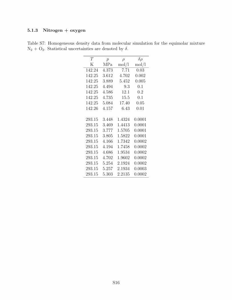
5.1.3 Nitrogen + oxygen

Table S7: Homogeneous density data from molecular simulation for the equimolar mixtureN2 + O2. Statistical uncertainties are denoted by δ.

T p ρ δρK MPa mol/l mol/l

142.24 4.373 7.71 0.03142.25 3.612 4.702 0.002142.25 3.889 5.452 0.005142.25 4.494 9.3 0.1142.25 4.586 12.1 0.2142.25 4.735 15.5 0.1142.25 5.084 17.40 0.05142.26 4.157 6.43 0.01

293.15 3.448 1.4324 0.0001293.15 3.469 1.4413 0.0001293.15 3.777 1.5705 0.0001293.15 3.805 1.5822 0.0001293.15 4.166 1.7342 0.0002293.15 4.194 1.7458 0.0002293.15 4.686 1.9534 0.0002293.15 4.702 1.9602 0.0002293.15 5.254 2.1924 0.0002293.15 5.257 2.1934 0.0003293.15 5.303 2.2135 0.0002

S16

Tab

leS8:

Vap

or-l

iquid

equilib

rium

dat

afr

omm

olec

ula

rsi

mula

tion

for

N2

+O

2.

Sta

tist

ical

unce

rtai

nti

esar

eden

oted

byδ.

Tp

δpxN2

y N2

δyN2

ρliq

δρliq

ρvap

δρvap

∆hres

vδ∆

hres

v

KM

Pa

MP

am

ol/m

olm

ol/m

olm

ol/m

olm

ol/l

mol

/lm

ol/l

mol

/lkJ/m

olkJ/m

ol80

0.04

00.

001

0.05

0.24

0.01

36.8

440.

005

0.06

10.

002

7.09

20.

001

800.

044

0.00

10.

100.

380.

0136.3

380.

004

0.06

80.

002

7.00

30.

001

800.

057

0.00

20.

200.

570.

0135.3

330.

005

0.08

80.

003

6.82

30.

001

800.

066

0.00

30.

300.

670.

0134.3

760.

005

0.10

10.

004

6.65

10.

001

800.

077

0.00

20.

400.

752

0.00

833.4

390.

004

0.11

90.

004

6.47

90.

001

800.

095

0.00

20.

500.

820

0.00

532.5

560.

004

0.14

80.

003

6.31

00.

001

800.

101

0.00

20.

600.

863

0.00

431.6

850.

005

0.15

80.

003

6.15

10.

001

800.

108

0.00

20.

700.

905

0.00

330.8

260.

005

0.16

80.

004

5.99

10.

001

800.

117

0.00

20.

800.

941

0.00

130.0

020.

004

0.18

30.

003

5.83

40.

001

800.

129

0.00

20.

900.

973

0.00

129.2

220.

005

0.20

40.

003

5.68

20.

001

105

0.42

70.

002

0.05

0.13

10.

001

32.7

720.

006

0.53

40.

003

6.22

40.

001

105

0.45

90.

002

0.10

0.23

60.

002

32.2

340.

005

0.57

70.

003

6.11

80.

001

105

0.53

10.

003

0.20

0.40

30.

003

31.1

610.

006

0.67

70.

003

5.89

80.

001

105

0.60

80.

002

0.30

0.52

40.

002

30.1

690.

006

0.78

70.

003

5.68

80.

001

105

0.68

80.

003

0.40

0.62

60.

002

29.1

720.

007

0.90

60.

003

5.47

20.

002

105

0.81

20.

003

0.60

0.77

70.

001

27.2

380.

006

1.09

80.

004

5.06

40.

002

105

0.95

50.

003

0.80

0.89

80.

001

25.3

800.

007

1.33

30.

004

4.64

90.

002

105

1.03

10.

004

0.90

0.95

10.

001

24.4

60.

011.

469

0.00

54.

436

0.00

3

120

1.10

80.

003

0.05

0.09

90.

001

29.9

070.

008

1.32

40.

004

5.49

40.

002

120

1.19

40.

005

0.10

0.19

00.

001

29.3

60.

011.

448

0.00

55.

362

0.00

312

01.

340

0.00

30.

200.

339

0.00

128.2

210.

009

1.66

60.

004

5.09

90.

003

120

1.48

00.

004

0.30

0.45

80.

002

27.1

20.

011.

887

0.00

54.

842

0.00

312

01.

632

0.00

40.

400.

560

0.00

226.0

20.

012.

144

0.00

64.

571

0.00

412

01.

750.

010.

500.

646

0.00

224.9

20.

022.

354

0.00

74.

318

0.00

412

01.

900.

010.

600.

724

0.00

123.8

10.

022.

636

0.00

74.

040.

0112

02.

050.

010.

700.

797

0.00

122.7

20.

012.

942

0.00

73.

757

0.00

512

02.

190.

010.

800.

868

0.00

121.5

50.

023.

270.

013.

460.

0112

02.

350.

010.

900.

936

0.00

120.3

40.

023.

661

0.00

93.

140.

01

S17

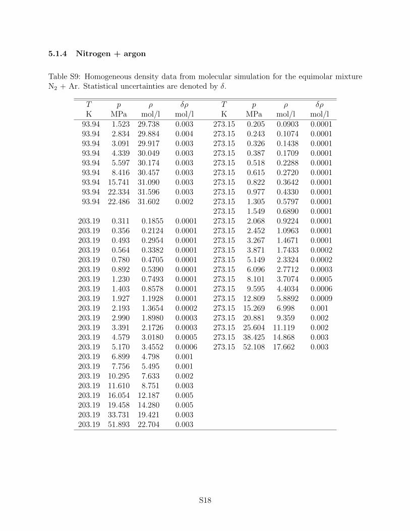
5.1.4 Nitrogen + argon

Table S9: Homogeneous density data from molecular simulation for the equimolar mixtureN2 + Ar. Statistical uncertainties are denoted by δ.

T p ρ δρ T p ρ δρK MPa mol/l mol/l K MPa mol/l mol/l

93.94 1.523 29.738 0.003 273.15 0.205 0.0903 0.000193.94 2.834 29.884 0.004 273.15 0.243 0.1074 0.000193.94 3.091 29.917 0.003 273.15 0.326 0.1438 0.000193.94 4.339 30.049 0.003 273.15 0.387 0.1709 0.000193.94 5.597 30.174 0.003 273.15 0.518 0.2288 0.000193.94 8.416 30.457 0.003 273.15 0.615 0.2720 0.000193.94 15.741 31.090 0.003 273.15 0.822 0.3642 0.000193.94 22.334 31.596 0.003 273.15 0.977 0.4330 0.000193.94 22.486 31.602 0.002 273.15 1.305 0.5797 0.0001

273.15 1.549 0.6890 0.0001203.19 0.311 0.1855 0.0001 273.15 2.068 0.9224 0.0001203.19 0.356 0.2124 0.0001 273.15 2.452 1.0963 0.0001203.19 0.493 0.2954 0.0001 273.15 3.267 1.4671 0.0001203.19 0.564 0.3382 0.0001 273.15 3.871 1.7433 0.0002203.19 0.780 0.4705 0.0001 273.15 5.149 2.3324 0.0002203.19 0.892 0.5390 0.0001 273.15 6.096 2.7712 0.0003203.19 1.230 0.7493 0.0001 273.15 8.101 3.7074 0.0005203.19 1.403 0.8578 0.0001 273.15 9.595 4.4034 0.0006203.19 1.927 1.1928 0.0001 273.15 12.809 5.8892 0.0009203.19 2.193 1.3654 0.0002 273.15 15.269 6.998 0.001203.19 2.990 1.8980 0.0003 273.15 20.881 9.359 0.002203.19 3.391 2.1726 0.0003 273.15 25.604 11.119 0.002203.19 4.579 3.0180 0.0005 273.15 38.425 14.868 0.003203.19 5.170 3.4552 0.0006 273.15 52.108 17.662 0.003203.19 6.899 4.798 0.001203.19 7.756 5.495 0.001203.19 10.295 7.633 0.002203.19 11.610 8.751 0.003203.19 16.054 12.187 0.005203.19 19.458 14.280 0.005203.19 33.731 19.421 0.003203.19 51.893 22.704 0.003

S18

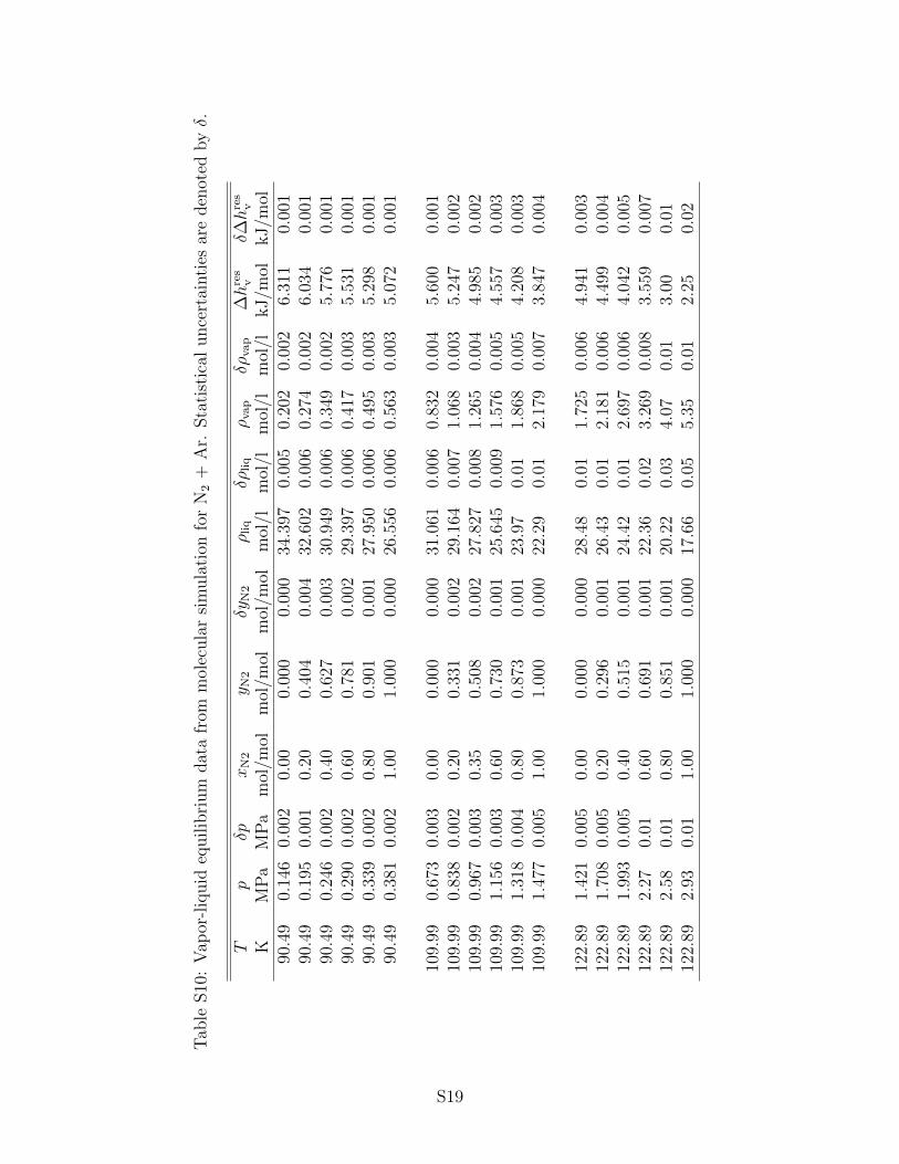
Tab

leS10

:V

apor

-liq

uid

equilib

rium

dat

afr

omm

olec

ula

rsi

mula

tion

for

N2

+A

r.Sta

tist

ical

unce

rtai

nti

esar

eden

oted

byδ.

Tp

δpxN2

y N2

δyN2

ρliq

δρliq

ρvap

δρvap

∆hres

vδ∆

hres

v

KM

Pa

MP

am

ol/m

olm

ol/m

olm

ol/m

olm

ol/l

mol

/lm

ol/l

mol

/lkJ/m

olkJ/m

ol90.4

90.

146

0.00

20.

000.

000

0.00

034.3

970.

005

0.20

20.

002

6.31

10.

001

90.4

90.

195

0.00

10.

200.

404

0.00

432.6

020.

006

0.27

40.

002

6.03

40.

001

90.4

90.

246

0.00

20.

400.

627

0.00

330.9

490.

006

0.34

90.

002

5.77

60.

001

90.4

90.

290

0.00

20.

600.

781

0.00

229.3

970.

006

0.41

70.

003

5.53

10.

001

90.4

90.

339

0.00

20.

800.

901

0.00

127.9

500.

006

0.49

50.

003

5.29

80.

001

90.4

90.

381

0.00

21.

001.

000

0.00

026.5

560.

006

0.56

30.

003

5.07

20.

001

109.

990.

673

0.00

30.

000.

000

0.00

031.0

610.

006

0.83

20.

004

5.60

00.

001

109.

990.

838

0.00

20.

200.

331

0.00

229.1

640.

007

1.06

80.

003

5.24

70.

002

109.

990.

967

0.00

30.

350.

508

0.00

227.8

270.

008

1.26

50.

004

4.98

50.

002

109.

991.

156

0.00

30.

600.

730

0.00

125.6

450.

009

1.57

60.

005

4.55

70.

003

109.

991.

318

0.00

40.

800.

873

0.00

123.9

70.

011.

868

0.00

54.

208

0.00

310

9.99

1.47

70.

005

1.00

1.00

00.

000

22.2

90.

012.

179

0.00

73.

847

0.00

4

122.

891.

421

0.00

50.

000.

000

0.00

028.4

80.

011.

725

0.00

64.

941

0.00

312

2.89

1.70

80.

005

0.20

0.29

60.

001

26.4

30.

012.

181

0.00

64.

499

0.00

412

2.89

1.99

30.

005

0.40

0.51

50.

001

24.4

20.

012.

697

0.00

64.

042

0.00

512

2.89

2.27

0.01

0.60

0.69

10.

001

22.3

60.

023.

269

0.00

83.

559

0.00

712

2.89

2.58

0.01

0.80

0.85

10.

001

20.2

20.

034.

070.

013.

000.

0112

2.89

2.93

0.01

1.00

1.00

00.

000

17.6

60.

055.

350.

012.

250.

02

S19

5.1.5 Argon + oxygen

Table S11: Homogeneous density data from molecular simulation for the equimolar mixtureAr + O2. Statistical uncertainties are denoted by δ.

T p ρ δρK MPa mol/l mol/l

298.1 3.040 1.2470 0.0001298.1 3.546 1.4583 0.0001298.1 4.053 1.6708 0.0002298.1 4.560 1.8840 0.0002298.1 5.066 2.0982 0.0002298.1 5.573 2.3126 0.0002298.1 6.080 2.5278 0.0003298.1 6.586 2.7443 0.0003298.1 7.093 2.9606 0.0004298.1 7.599 3.1782 0.0004298.1 8.106 3.3958 0.0004298.1 8.613 3.6135 0.0005298.1 9.119 3.8317 0.0005298.1 9.626 4.0497 0.0006298.1 10.133 4.2678 0.0005298.1 10.639 4.4867 0.0007298.1 11.146 4.7060 0.0007298.1 11.652 4.9253 0.0008298.1 12.159 5.1429 0.0009298.1 12.666 5.3604 0.0009

S20

Tab

leS12

:V

apor

-liq

uid

equilib

rium

dat

afr

omm

olec

ula

rsi

mula

tion

for

Ar

+O

2.

Sta

tist

ical

unce

rtai

nti

esar

eden

oted

byδ.

Tp

δpxAr

y Ar

δyAr

ρliq

δρliq

ρvap

δρvap

∆hres

vδ∆

hres

v

KM

Pa

MP

am

ol/m

olm

ol/m

olm

ol/m

olm

ol/l

mol

/lm

ol/l

mol

/lkJ/m

olkJ/m

ol90

0.10

20.

002

0.00

00.

000

0.00

035

.805

0.00

50.

140

0.00

26.

877

0.00

190

0.11

30.

001

0.23

00.

295

0.00

435

.505

0.00

50.

156

0.00

26.

728

0.00

190

0.11

80.

001

0.44

20.

516

0.00

535

.217

0.00

50.

163

0.00

26.

604

0.00

190

0.12

80.

001

0.65

00.

710

0.00

434

.934

0.00

50.

177

0.00

26.

489

0.00

190

0.13

50.

001

0.83

40.

867

0.00

234

.690

0.00

50.

187

0.00

26.

399

0.00

190

0.14

10.

002

1.00

01.

000

0.00

034

.479

0.00

40.

196

0.00

26.

326

0.00

1

104.

510.

369

0.00

30.

000

0.00

00.

000

33.3

880.

005

0.45

90.

003

6.35

30.

001

104.

510.

387

0.00

20.

146

0.17

80.

001

33.1

950.

006

0.48

20.

002

6.26

20.

001

104.

510.

417

0.00

20.

413

0.46

60.

002

32.8

290.

006

0.52

30.

002

6.10

50.

001

104.

510.

437

0.00

20.

608

0.65

30.

002

32.5

690.

007

0.55

00.

002

6.00

20.

001

104.

510.

451

0.00

30.

750

0.78

10.

002

32.3

810.

006

0.56

90.

003

5.93

30.

001

104.

510.

471

0.00

21.

000

1.00

00.

000

32.0

490.

006

0.59

50.

003

5.82

40.

001

120.

021.

051

0.00

30.

000

0.00

00.

000

30.4

980.

009

1.24

60.

004

5.61

70.

002

120.

021.

078

0.00

30.

159

0.17

90.

001

30.2

630.

007

1.28

10.

004

5.52

30.

002

120.

021.

123

0.00

30.

380

0.41

30.

001

29.9

510.

009

1.34

20.

004

5.39

70.

002

120.

021.

160

0.00

30.

565

0.59

40.

002

29.6

840.

006

1.39

60.

003

5.29

70.

002

120.

021.

191

0.00

30.

773

0.79

00.

001

29.3

970.

008

1.43

80.

003

5.20

10.

002

120.

021.

222

0.00

41.

000

1.00

00.

000

29.0

970.

009

1.48

30.

005

5.10

60.

002

S21

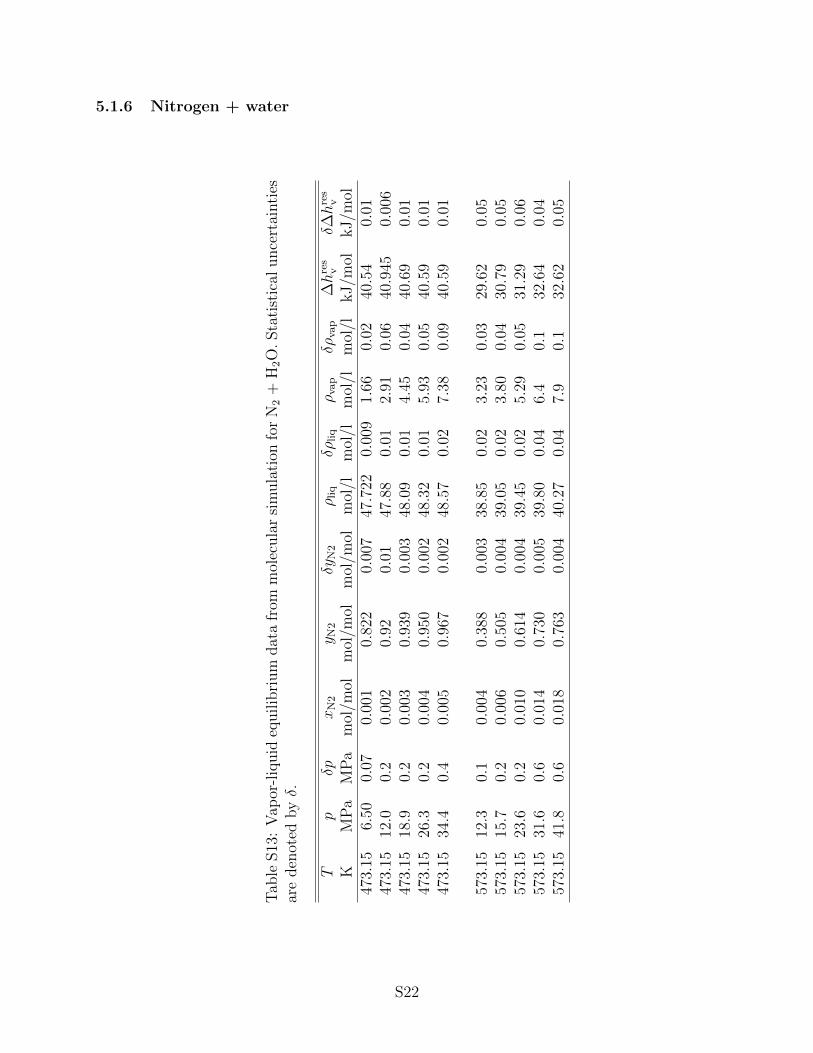
5.1.6 Nitrogen + water

Tab

leS13

:V

apor

-liq

uid

equilib

rium

dat

afr

omm

olec

ula

rsi

mula

tion

for

N2

+H

2O

.Sta

tist

ical

unce

rtai

nti

esar

eden

oted

byδ.

Tp

δpxN2

y N2

δyN2

ρliq

δρliq

ρvap

δρvap

∆hres

vδ∆

hres

v

KM

Pa

MP

am

ol/m

olm

ol/m

olm

ol/m

olm

ol/l

mol

/lm

ol/l

mol

/lkJ/m

olkJ/m

ol47

3.15

6.50

0.07

0.00

10.

822

0.00

747.7

220.

009

1.66

0.02

40.5

40.

0147

3.15

12.0

0.2

0.00

20.

920.

0147.8

80.

012.

910.

0640.9

450.

006

473.

1518.9

0.2

0.00

30.

939

0.00

348.0

90.

014.

450.

0440.6

90.

0147

3.15

26.3

0.2

0.00

40.

950

0.00

248.3

20.

015.

930.

0540.5

90.

0147

3.15

34.4

0.4

0.00

50.

967

0.00

248.5

70.

027.

380.

0940.5

90.

01

573.

1512.3

0.1

0.00

40.

388

0.00

338.8

50.

023.

230.

0329.6

20.

0557

3.15

15.7

0.2

0.00

60.

505

0.00

439.0

50.

023.

800.

0430.7

90.

0557

3.15

23.6

0.2

0.01

00.

614

0.00

439.4

50.

025.

290.

0531.2

90.

0657

3.15

31.6

0.6

0.01

40.

730

0.00

539.8

00.

046.

40.

132.6

40.

0457

3.15

41.8

0.6

0.01

80.

763

0.00

440.2

70.

047.

90.

132.6

20.

05

S22

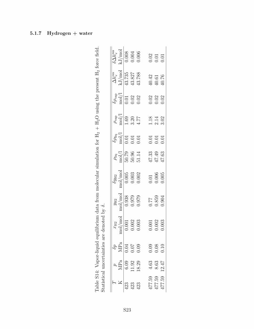
5.1.7 Hydrogen + water

Tab

leS14

:V

apor

-liq

uid

equilib

rium

dat

afr

omm

olec

ula

rsi

mula

tion

for

H2

+H

2O

usi

ng

the

pre

sent

H2

forc

efiel

d.

Sta

tist

ical

unce

rtai

nti

esar

eden

oted

byδ.

Tp

δpxH2

y H2

δyH2

ρliq

δρliq

ρvap

δρvap

∆hres

vδ∆

hres

v

KM

Pa

MP

am

ol/m

olm

ol/m

olm

ol/m

olm

ol/l

mol

/lm

ol/l

mol

/lkJ/m

olkJ/m

ol42

36.

090.

040.

001

0.93

80.

005

50.7

90.

011.

690.

0143.7

350.

008

423

11.9

20.

070.

002

0.97

90.

003

50.9

60.

013.

200.

0243.8

270.

004

423

18.2

90.

090.

003

0.97

90.

002

51.1

40.

014.

770.

0243.7

880.

006

477.

594.

630.

090.

001

0.77

0.01

47.3

30.

011.

180.

0240.4

20.

0247

7.59

8.63

0.08

0.00

20.

859

0.00

647.4

90.

012.

140.

0240.6

10.

0147

7.59

12.4

70.

100.

003

0.90

40.

005

47.6

30.

013.

020.

0240.7

60.

01

S23

Tab

leS15

:V

apor

-liq

uid

equilib

rium

dat

afr

omm

olec

ula

rsi

mula

tion

for

H2

+H

2O

usi

ng

the

H2

forc

efiel

dof

Mar

xan

dN

iela

baS1.

Sta

tist

ical

unce

rtai

nti

esar

eden

oted

byδ.

Tp

δpxH2

y H2

δyH2

ρliq

δρliq

ρvap

δρvap

∆hres

vδ∆

hres

v

KM

Pa

MP

am

ol/m

olm

ol/m

olm

ol/m

olm

ol/l

mol

/lm

ol/l

mol

/lkJ/m

olkJ/m

ol42

35.

710.

030.

001

0.94

80.

004

50.7

930.

009

1.59

0.01

43.7

560.

007

423

11.1

10.

050.

002

0.99

70.

002

50.9

490.

009

3.01

0.01

43.8

040.

003

423

17.1

10.

090.

003

0.98

50.

001

51.1

20.

014.

520.

0243.7

360.

005

477.

594.

490.

070.

001

0.76

0.01

47.3

70.

011.

150.

0240.3

50.

0147

7.59

8.07

0.07

0.00

20.

863

0.00

747.5

00.

012.

010.

0240.6

40.

0147

7.59

11.8

0.1

0.00

30.

908

0.00

647.6

30.

012.

870.

0240.7

640.

009

S24

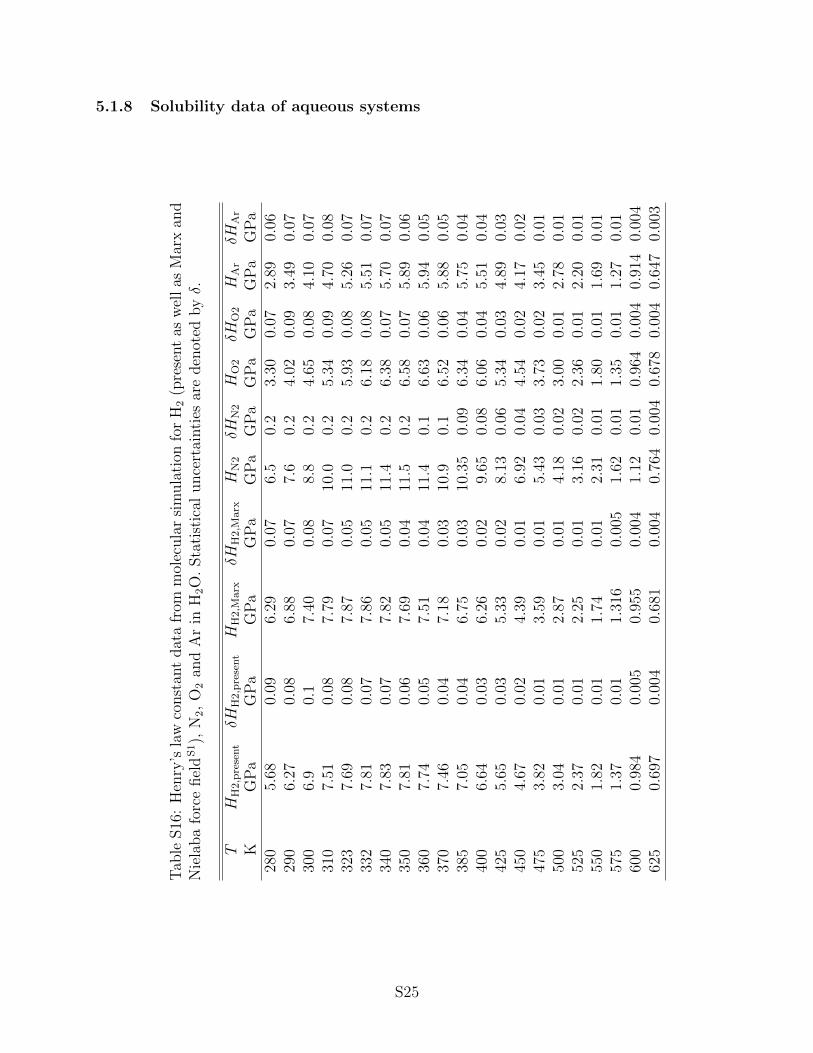
5.1.8 Solubility data of aqueous systems

Tab

leS16

:H

enry

’sla

wco

nst

ant

dat

afr

omm

olec

ula

rsi

mula

tion

for

H2

(pre

sent

asw

ell

asM

arx

and

Nie

laba

forc

efiel

dS1),

N2,

O2

and

Ar

inH

2O

.Sta

tist

ical

unce

rtai

nti

esar

eden

oted

byδ.

TH

H2,present

δHH2,present

HH2,M

arx

δHH2,M

arx

HN2

δHN2

HO2

δHO2

HAr

δHAr

KG

Pa

GP

aG

Pa

GP

aG

Pa

GP

aG

Pa

GP

aG

Pa

GP

a28

05.

680.

096.

290.

076.

50.

23.

300.

072.

890.

0629

06.

270.

086.

880.

077.

60.

24.

020.

093.

490.

0730

06.

90.

17.

400.

088.

80.

24.

650.

084.

100.

0731

07.

510.

087.

790.

0710.0

0.2

5.34

0.09

4.70

0.08

323

7.69

0.08

7.87

0.05

11.0

0.2

5.93

0.08

5.26

0.07

332

7.81

0.07

7.86

0.05

11.1

0.2

6.18

0.08

5.51

0.07

340

7.83

0.07

7.82

0.05

11.4

0.2

6.38

0.07

5.70

0.07

350

7.81

0.06

7.69

0.04

11.5

0.2

6.58

0.07

5.89

0.06

360

7.74

0.05

7.51

0.04

11.4

0.1

6.63

0.06

5.94

0.05

370

7.46

0.04

7.18

0.03

10.9

0.1

6.52

0.06

5.88

0.05

385

7.05

0.04

6.75

0.03

10.3

50.

096.

340.

045.

750.

0440

06.

640.

036.

260.

029.

650.

086.

060.

045.

510.

0442

55.

650.

035.

330.

028.

130.

065.

340.

034.

890.

0345

04.

670.

024.

390.

016.

920.

044.

540.

024.

170.

0247

53.

820.

013.

590.

015.

430.

033.

730.

023.

450.

0150

03.

040.

012.

870.

014.

180.

023.

000.

012.

780.

0152

52.

370.

012.

250.

013.

160.

022.

360.

012.

200.

0155

01.

820.

011.

740.

012.

310.

011.

800.

011.

690.

0157

51.

370.

011.

316

0.00

51.

620.

011.

350.

011.

270.

0160

00.

984

0.00

50.

955

0.00

41.

120.

010.

964

0.00

40.

914

0.00

462

50.

697

0.00

40.

681

0.00

40.

764

0.00

40.

678

0.00

40.

647

0.00

3

S25

5.2 Ternary mixtures

5.2.1 Nitrogen + oxygen + argon

Table S17: Homogeneous density data from molecular simulation for N2 + O2 + Ar at thecomposition of ambient air xN2 = 0.781, xO2 = 0.210 and xAr = 0.009 mol/mol. Statisticaluncertainties are denoted by δ.

T p ρ δρ T p ρ δρK MPa mol/l mol/l K MPa mol/l mol/l

70 3.510 32.000 0.003 873.19 1.555 0.2131 0.000170 6.930 32.205 0.003 873.19 10.170 1.3496 0.000170 10.220 32.396 0.003 873.19 22.290 2.8309 0.000270 13.990 32.609 0.003 873.19 34.090 4.1506 0.000370 17.370 32.786 0.003 873.19 41.550 4.9292 0.000470 20.520 32.945 0.003 873.19 48.220 5.5925 0.000570 24.340 33.134 0.002 873.19 55.620 6.2927 0.000570 28.340 33.321 0.003 873.19 100.000 9.8648 0.0008

873.19 150.000 12.9477 0.0009473.15 2.473 0.6232 0.0001 873.19 200.000 15.388 0.001473.15 5.069 1.2642 0.0001 873.19 250.000 17.396 0.001473.15 10.004 2.4433 0.0002 873.19 300.000 19.094 0.001473.15 14.620 3.4955 0.0003 873.19 350.000 20.566 0.001473.15 20.540 4.7695 0.0005 873.19 400.000 21.861 0.001473.15 26.450 5.9578 0.0007 873.19 450.000 23.020 0.001473.15 33.910 7.3409 0.0008 873.19 500.000 24.066 0.001473.15 40.890 8.525 0.001473.15 51.390 10.122 0.001 1500 100.000 6.4245 0.0005473.15 61.860 11.527 0.001 1500 150.000 8.7916 0.0007473.15 69.470 12.450 0.001 1500 200.000 10.8034 0.0009473.15 100.000 15.497 0.002 1500 250.000 12.5428 0.0009473.15 150.000 19.049 0.001 1500 300.000 14.076 0.001473.15 200.000 21.606 0.001 1500 350.000 15.442 0.001473.15 250.000 23.601 0.001 1500 400.000 16.674 0.001473.15 300.000 25.235 0.001 1500 450.000 17.795 0.001473.15 350.000 26.619 0.001 1500 500.000 18.824 0.001473.15 400.000 27.821 0.001473.15 450.000 28.885 0.001473.15 500.000 29.838 0.001

S26

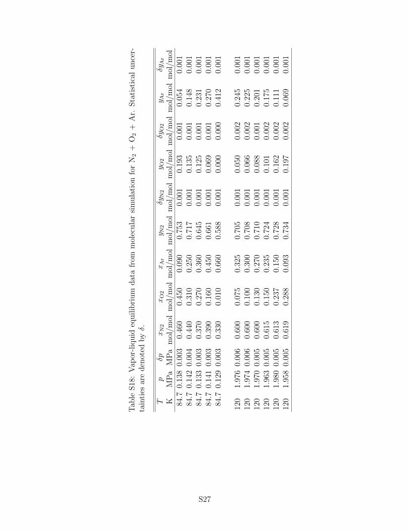
Tab

leS18

:V

apor

-liq

uid

equilib

rium

dat

afr

omm

olec

ula

rsi

mula

tion

for

N2

+O

2+

Ar.

Sta

tist

ical

unce

r-ta

inti

esar

eden

oted

byδ.

Tp

δpxN2

xO2

xAr

y N2

δyN2

y O2

δyO2

y Ar

δyAr

KM

Pa

MP

am

ol/m

olm

ol/m

olm

ol/m

olm

ol/m

olm

ol/m

olm

ol/m

olm

ol/m

olm

ol/m

olm

ol/m

ol84

.70.

138

0.00

30.

460

0.45

00.

090

0.75

30.

001

0.19

30.

001

0.05

40.

001

84.7

0.14

20.

004

0.44

00.

310

0.25

00.

717

0.00

10.

135

0.00

10.

148

0.00

184

.70.

133

0.00

30.

370

0.27

00.

360

0.64

50.

001

0.12

50.

001

0.23

10.

001

84.7

0.14

10.

003

0.39

00.

160

0.45

00.

661

0.00

10.

069

0.00

10.

270

0.00

184

.70.

129

0.00

30.

330

0.01

00.

660

0.58

80.

001

0.00

00.

000

0.41

20.

001

120

1.97

60.

006

0.60

00.

075

0.32

50.

705

0.00

10.

050

0.00

20.

245

0.00

112

01.

974

0.00

60.

600

0.10

00.

300

0.70

80.

001

0.06

60.

002

0.22

50.

001

120

1.97

00.

005

0.60

00.

130

0.27

00.

710

0.00

10.

088

0.00

10.

201

0.00

112

01.

963

0.00

50.

615

0.15

00.

235

0.72

40.

001

0.10

10.

002

0.17

50.

001

120

1.98

00.

005

0.61

30.

237

0.15

00.

728

0.00

10.

162

0.00

20.

111

0.00

112

01.

958

0.00

50.

619

0.28

80.

093

0.73

40.

001

0.19

70.

002

0.06

90.

001

S27

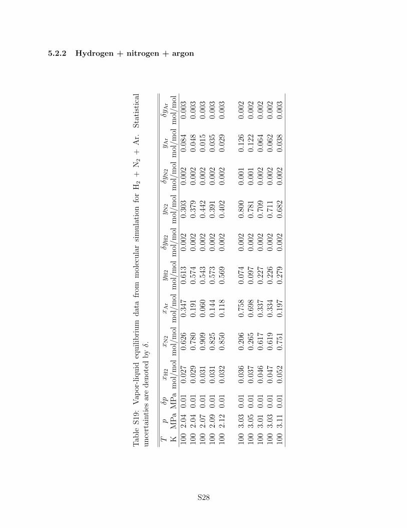
5.2.2 Hydrogen + nitrogen + argon

Tab

leS19

:V

apor

-liq

uid

equilib

rium

dat

afr

omm

olec

ula

rsi

mula

tion

for

H2

+N

2+

Ar.

Sta

tist

ical

unce

rtai

nti

esar

eden

oted

byδ.

Tp

δpxH2

xN2

xAr

y H2

δyH2

y N2

δyN2

y Ar

δyAr

KM

Pa

MP

am

ol/m

olm

ol/m

olm

ol/m

olm

ol/m

olm

ol/m

olm

ol/m

olm

ol/m

olm

ol/m

olm

ol/m

ol10

02.

040.

010.

027

0.62

60.

347

0.61

30.

002

0.30

30.

002

0.08

40.

003

100

2.04

0.01

0.02

90.

780

0.19

10.

574

0.00

20.

379

0.00

20.

048

0.00

310

02.

070.

010.

031

0.90

90.

060

0.54

30.

002

0.44

20.

002

0.01

50.

003

100

2.09

0.01

0.03

10.

825

0.14

40.

573

0.00

20.

391

0.00

20.

035

0.00

310

02.

120.

010.

032

0.85

00.

118

0.56

90.

002

0.40

20.

002

0.02

90.

003

100

3.03

0.01

0.03

60.

206

0.75

80.

074

0.00

20.

800

0.00

10.

126

0.00

210

03.

050.

010.

037

0.26

50.

698

0.09

70.

002

0.78

10.

001

0.12

20.

002

100

3.01

0.01

0.04

60.

617

0.33

70.

227

0.00

20.

709

0.00

20.

064

0.00

210

03.

030.

010.

047

0.61

90.

334

0.22

60.

002

0.71

10.

002

0.06

20.

002

100

3.11

0.01

0.05

20.

751

0.19

70.

279

0.00

20.

682

0.00

20.

038

0.00

3

S28

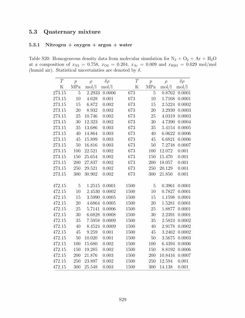
5.3 Quaternary mixture

5.3.1 Nitrogen + oxygen + argon + water

Table S20: Homogeneous density data from molecular simulation for N2 + O2 + Ar + H2Oat a composition of xN2 = 0.758, xO2 = 0.204, xAr = 0.009 and xH2O = 0.029 mol/mol(humid air). Statistical uncertainties are denoted by δ.

T p ρ δρ T p ρ δρK MPa mol/l mol/l K MPa mol/l mol/l

273.15 5 2.2933 0.0006 673 5 0.8762 0.0001273.15 10 4.628 0.001 673 10 1.7168 0.0001273.15 15 6.872 0.002 673 15 2.5224 0.0002273.15 20 8.932 0.002 673 20 3.2939 0.0003273.15 25 10.746 0.002 673 25 4.0319 0.0003273.15 30 12.323 0.002 673 30 4.7390 0.0004273.15 35 13.686 0.003 673 35 5.4154 0.0005273.15 40 14.864 0.003 673 40 6.0622 0.0006273.15 45 15.899 0.003 673 45 6.6821 0.0006273.15 50 16.816 0.003 673 50 7.2748 0.0007273.15 100 22.521 0.002 673 100 12.072 0.001273.15 150 25.654 0.002 673 150 15.470 0.001273.15 200 27.837 0.002 673 200 18.057 0.001273.15 250 29.521 0.002 673 250 20.129 0.001273.15 300 30.902 0.002 673 300 21.850 0.001

472.15 5 1.2515 0.0001 1500 5 0.3961 0.0001472.15 10 2.4530 0.0002 1500 10 0.7827 0.0001472.15 15 3.5990 0.0005 1500 15 1.1598 0.0001472.15 20 4.6864 0.0005 1500 20 1.5281 0.0001472.15 25 5.7141 0.0006 1500 25 1.8877 0.0001472.15 30 6.6828 0.0008 1500 30 2.2391 0.0001472.15 35 7.5958 0.0009 1500 35 2.5824 0.0002472.15 40 8.4524 0.0009 1500 40 2.9178 0.0002472.15 45 9.259 0.001 1500 45 3.2462 0.0002472.15 50 10.020 0.001 1500 50 3.5675 0.0003472.15 100 15.680 0.002 1500 100 6.4394 0.0006472.15 150 19.285 0.002 1500 150 8.8192 0.0006472.15 200 21.876 0.003 1500 200 10.8416 0.0007472.15 250 23.897 0.002 1500 250 12.594 0.001472.15 300 25.548 0.003 1500 300 14.138 0.001

S29

Table S21: Homogeneous density data from molecular simulation for N2 + O2 + Ar + H2Oat a composition of xN2 = 0.163, xO2 = 0.044, xAr = 0.002 and xH2O = 0.791 mol/mol(supercritical H2O containing ≈ 0.2 mol/mol of air components). Statistical uncertaintiesare denoted by δ.

T p ρ δρK MPa mol/l mol/l

672.95 33.3 9.53 0.01672.95 52.2 15.74 0.01672.95 80.9 21.92 0.01672.95 118.6 26.78 0.01672.95 172.6 31.21 0.01672.95 214.2 33.61 0.01672.95 233.0 34.54 0.01672.95 249.3 35.26 0.01672.95 279.5 36.51 0.01

S30

References

(S1) Marx, D.; Nielaba, P. Path-integral Monte Carlo techniques for rotational motion in

two dimensions: Quenched, annealed, and no-spin quantum-statistical averages. Phys.

Rev. A 1992, 45, 8968–8971.

(S2) Fastovskii, V. G.; Petrovskii, Y. V. A study of the vapor-liquid equilibrium in the

system oxygen-argon-nitrogen. Zh. Fiz. Khim. 1957, 31, 836–841.

(S3) Xiao, J.; Liu, K. Measurement and correlation of vapor - liquid equilibrium data in

H2 - N2 - Ar system. J. Chem. Eng. (China) 1990, 8, 8–12.

(S4) Kunz, O.; Wagner, W. The GERG-2008 wide-range equation of state for natural

gases and other mixtures: an expansion of GERG-2004. J. Chem. Eng. Data 2012,

57, 3032–3091.

(S5) Eubanks, L. S. Vapor-Liquid equilibria in the system Hydrogen-Nitrogen-Carbon

monoxide. Ph.D. thesis, Rice University, 1957.

(S6) Akers, W. W.; Eubanks, L. S. Vapor-Liquid Equilibria in the System Hydrogen-

Nitrogen-Carbon Monoxide. Adv. Cryog. Eng. 1960, 3, 275–293.

(S7) Streett, W. B.; Calado, J. C. G. Liquid-vapour equilibrium for hydrogen + nitrogen

at temperatures from 63 to 110 K and pressures to 57 MPa. J. Chem. Thermodyn.

1978, 10, 1089–1100.

(S8) Calado, J. C. G.; Streett, W. B. Liquid-vapor equilibrium in the system H2 + Ar at

temperatures from 83 to 141 K and pressures to 52 MPa. Fluid Phase Equilib. 1979,

2, 275–282.

(S9) Ostronov, M. G.; Shatskaya, L. V.; Finyagina, R. A.; Brodskaya, L. F.; Zhirnova, N. A.

Gas-Liquid Phase Equilibrium in the Argon-Hydrogen System at Intermediate Pres-

sures. Russ. J. Phys. Chem. 1977, 51, 1407–1409.

S31

(S10) Volk, H.; Halsey Jr., G. D. Solubility of hydrogen and deuterium in liquid argon. J.

Chem. Phys. 1960, 33, 1132–1139.

(S11) Mullins, J. C.; Ziegler, W. T. Phase equilibria in the argon-helium and argon-hydrogen

systems from 68 to 108 K and pressures to 120 atmospheres. Adv. Cryog. Eng. 1965,

10, 171–181.

(S12) International Association for the Properties of Water and Steam, Guideline on the

Henry’s Constant and Vapor-Liquid Distribution Constant for Gases in H2O and D2O

at High Temperatures . 2004.

(S13) Fernandez-Prini, R.; Alvarez, J. L.; Harvey, A. H. Henry’s constants and vapor–liquid

distribution constants for gaseous solutes in H2O and D2O at high temperatures. J.

Phys. Chem. Ref. Data 2003, 32, 903–916.

(S14) Morris, D. R.; Yang, L.; Giraudeau, F.; Sun, X.; Steward, F. R. Henry’s law constant

for hydrogen in natural water and deuterium in heavy water. Phys. Chem. Chem.

Phys. 2001, 3, 1043–1046.

(S15) Alvarez, J.; Fernandez-Prini, R. A semiempirical procedure to describe the thermo-

dynamics of dissolution of non-polar gases in water. Fluid Phase Equilib. 1991, 66,

309–326.

(S16) Rettich, T. R.; Battino, R.; Wilhelm, E. Solubility of gases in liquids. XVI. Henry’s

law coefficients for nitrogen in water at 5 to 50◦ C. J. Solution Chem. 1984, 13,

335–348.

(S17) Cosgrove, B. A.; Walkley, J. Solubilities of gases in H2O and 2H2O. J. Chromatogr. A

1981, 216, 161–167.

(S18) Alvarez, J.; Crovetto, R.; Fernandez-Prini, R. The dissolution of N2 and of H2 in water

from room temperature to 640 K. Ber. Bunsenges. Phys. Chem. 1988, 92, 935–940.

S32

(S19) Rettich, T. R.; Battino, R.; Wilhelm, E. Solubility of gases in liquids. 22. High-

precision determination of Henry’s law constants of oxygen in liquid water from T=

274 K to T= 328 K. J. Chem. Thermodyn. 2000, 32, 1145–1156.

(S20) Benson, B. B.; Krause, D.; Peterson, M. A. The solubility and isotopic fractionation

of gases in dilute aqueous solution. I. Oxygen. J. Solution Chem. 1979, 8, 655–690.

(S21) Rettich, T. R.; Handa, Y. P.; Battino, R.; Wilhelm, E. Solubility of gases in liquids. 13.

High-precision determination of Henry’s constants for methane and ethane in liquid

water at 275 to 328 K. J. Phys. Chem. 1981, 85, 3230–3237.

(S22) Cramer, S. D. The solubility of oxygen in brines from 0 to 300◦ C. Ind. Eng. Chem.

Process Des. Dev. 1980, 19, 300–305.

(S23) Rettich, T. R.; Battino, R.; Wilhelm, E. Solubility of gases in liquids. 18. High-

precision determination of Henry fugacities for argon in liquid water at 2 to 40◦ C. J.

Solution Chem. 1992, 21, 987–1004.

(S24) Krause, D.; Benson, B. B. The solubility and isotopic fractionation of gases in dilute

aqueous solution. IIa. Solubilities of the noble gases. J. Solution Chem. 1989, 18,

823–873.

(S25) Potter, R. W.; Clynne, M. A. The solubility of the noble gases He, Ne, Ar, Kr, and

Xe in water up to the critical point. J. Solution Chem. 1978, 7, 837–844.

(S26) Crovetto, R.; Fernandez-Prini, R.; Japas, M. L. Solubilities of inert gases and methane

in H2O and in D2O in the temperature range of 300 to 600 K. J. Chem. Phys. 1982,

76, 1077–1086.

S33