Mold Distortion Simulation of BB2 at SDI Lance C. Hibbeler and Brian G. Thomas

UIUC: CCC Report CCC200803

Aug.4, 2008

Model Description

The complete geometry of ¼ of the mold copper plates and water box was built as accurately as possible. It includes the curvature of the hot face and water channels, as well as the angled water channel entrance/exit ports in the web section of the beam blank. The water boxes were simplified, with only the overall shape, large features, and bolt holes included in the model. To be as efficient as possible, the meshes are mixed hexahedrons, wedges (triangle element projected into the third dimension), and tetrahedrons.

Heat Transfer Boundary Conditions

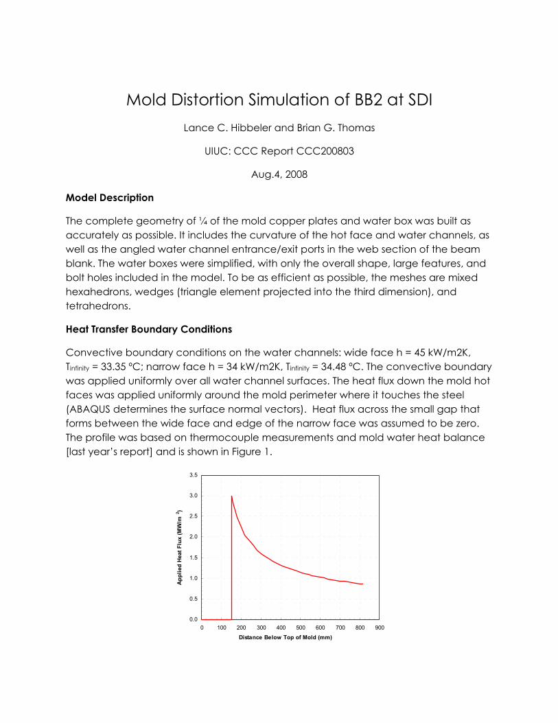
Convective boundary conditions on the water channels: wide face h = 45 kW/m2K, Tinfinity = 33.35 ºC; narrow face h = 34 kW/m2K, Tinfinity = 34.48 ºC. The convective boundary was applied uniformly over all water channel surfaces. The heat flux down the mold hot faces was applied uniformly around the mold perimeter where it touches the steel (ABAQUS determines the surface normal vectors). Heat flux across the small gap that forms between the wide face and edge of the narrow face was assumed to be zero. The profile was based on thermocouple measurements and mold water heat balance [last year’s report] and is shown in Figure 1.

0.0

0.5

1.0

1.5

2.0

2.5

3.0

3.5

0 100 200 300 400 500 600 700 800 900

Distance Below Top of Mold (mm)

App

lied

Hea

t Flu

x (M

W/m

2 )

Figure 1. Heat Flux Profile

Mechanical Boundary Conditions

The boundary conditions used in the mechanical analysis are shown in Figure 2 and Figure 3. Although the figures show the “full back” mold, the exact same conditions were applied to the “cut back” mold (where Accumold removed copper to insert the thermocouples). The proper boundary conditions were determined by iteratively placing constraint equations in the model at locations where the mold and water box pieces were penetrating each other. The mold narrow/wide face interface constrains the y-displacement to be equal at four points: the meniscus, the bottom edge, and at the level of the two rows of bolt holes between those two points. The mold/waterbox interfaces has the top and bottom edges constrained to equal displacement in the appropriate direction. The vertical edge of the wide face furthest away from the centerline is also constrained at its midpoint with the waterbox. The mold bolts were modeled in ABAQUS using assembly-level wires with an axial-only connector cross-section (essentially line elements) and ABAQUS “kinematic coupling constraints” that distributes the bolt load over appropriate regions in the mold and water box. Figure 4 explains the coupling constraints. The 70 ft-lbf torque applied to the 5/8 UNF bolts was converted to a 29 kN pre-load with the appropriate unit conversions and the equation [Shigley’s Mechanical Engineering Design]:

2 dFd dτ π μλ

λ πμ⎛ ⎞−= ⎜ ⎟+⎝ ⎠

(1)

Where F is the “clamping force”, τ is the torque, d is the nominal bolt diameter, λ is the thread pitch, and μ is the coefficient of friction, taken to be 0.38, but varies depending on lubrication. The 2.56” diameter tie rods, which are fastened with Bellevue washers (disc springs) to a large nut were preloaded assuming the same 70 ft-lbf torque, giving a 7.3 kN load. This is a reasonable value of the safety factor allowed over the net effect of the ferrostatic pressure. Neither the clamping forces nor ferrostatic pressure were included in the model (they were assumed to roughly cancel, based on previous work [Thomas et al, 1998]).

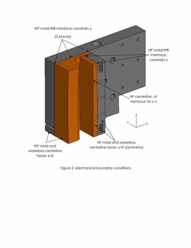
Figure 2. Mechanical boundary conditions

NF centerline, at meniscus: fix x, z

NF mold and waterbox centerline faces: y=0 (symmetry) WF mold and

waterbox centerline faces: x=0

NF mold/WB interface: constrain x

WF mold/WB interface: constrain y

(3 places)

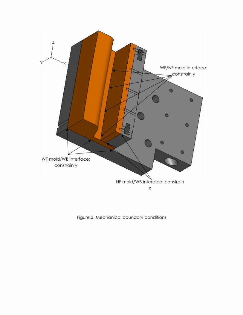
Figure 3. Mechanical boundary conditions

WF mold/WB interface: constrain y

NF mold/WB interface: constrain x

WF/NF mold interface: constrain y

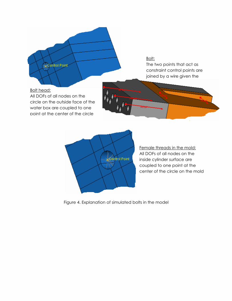
Figure 4. Explanation of simulated bolts in the model

Female threads in the mold: All DOFs of all nodes on the inside cylinder surface are coupled to one point at the center of the circle on the mold

Bolt head: All DOFs of all nodes on the circle on the outside face of the water box are coupled to one point at the center of the circle

Bolt: The two points that act as constraint control points are joined by a wire given the

Heat Transfer Results

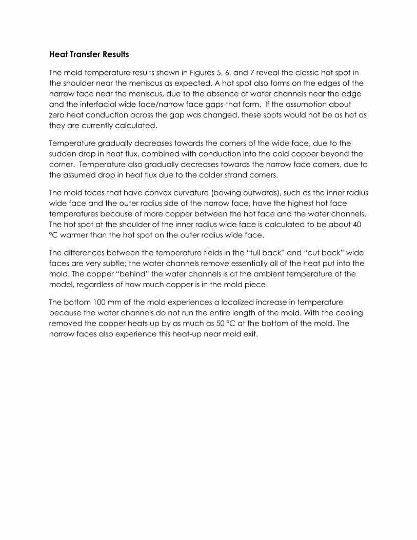
The mold temperature results shown in Figures 5, 6, and 7 reveal the classic hot spot in the shoulder near the meniscus as expected. A hot spot also forms on the edges of the narrow face near the meniscus, due to the absence of water channels near the edge and the interfacial wide face/narrow face gaps that form. If the assumption about zero heat conduction across the gap was changed, these spots would not be as hot as they are currently calculated.

Temperature gradually decreases towards the corners of the wide face, due to the sudden drop in heat flux, combined with conduction into the cold copper beyond the corner. Temperature also gradually decreases towards the narrow face corners, due to the assumed drop in heat flux due to the colder strand corners.

The mold faces that have convex curvature (bowing outwards), such as the inner radius wide face and the outer radius side of the narrow face, have the highest hot face temperatures because of more copper between the hot face and the water channels. The hot spot at the shoulder of the inner radius wide face is calculated to be about 40 ºC warmer than the hot spot on the outer radius wide face.

The differences between the temperature fields in the “full back” and “cut back” wide faces are very subtle; the water channels remove essentially all of the heat put into the mold. The copper “behind” the water channels is at the ambient temperature of the model, regardless of how much copper is in the mold piece.

The bottom 100 mm of the mold experiences a localized increase in temperature because the water channels do not run the entire length of the mold. With the cooling removed the copper heats up by as much as 50 ºC at the bottom of the mold. The narrow faces also experience this heat-up near mold exit.

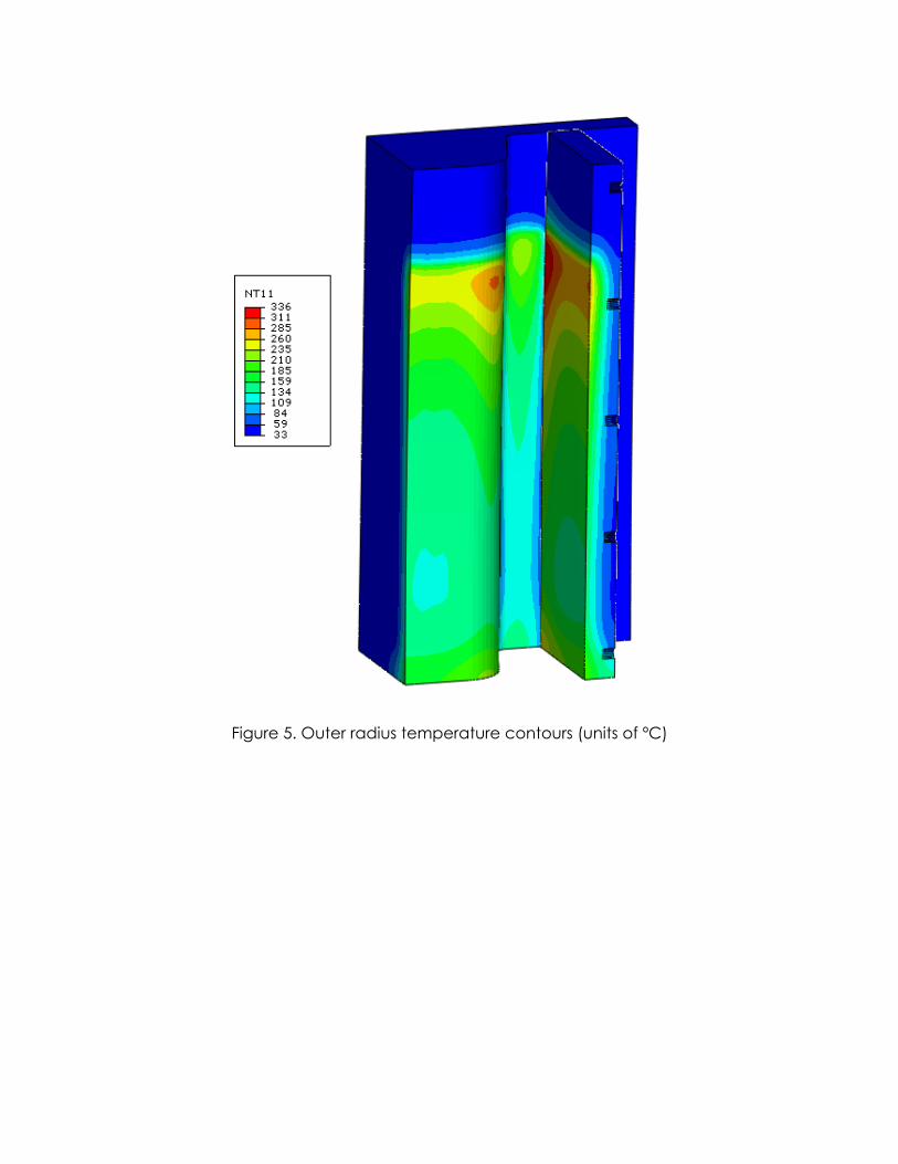
Figure 5. Outer radius temperature contours (units of ºC)

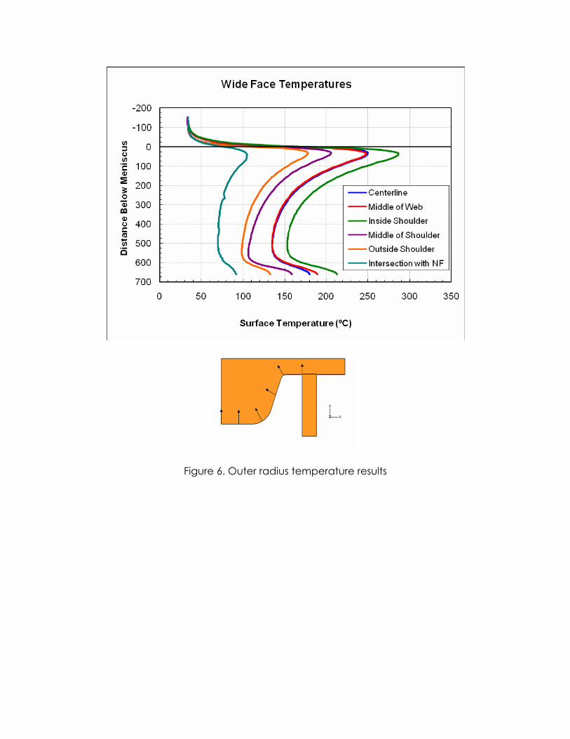
Figure 6. Outer radius temperature results

Figure 7. Outer radius side of narrow face temperature results

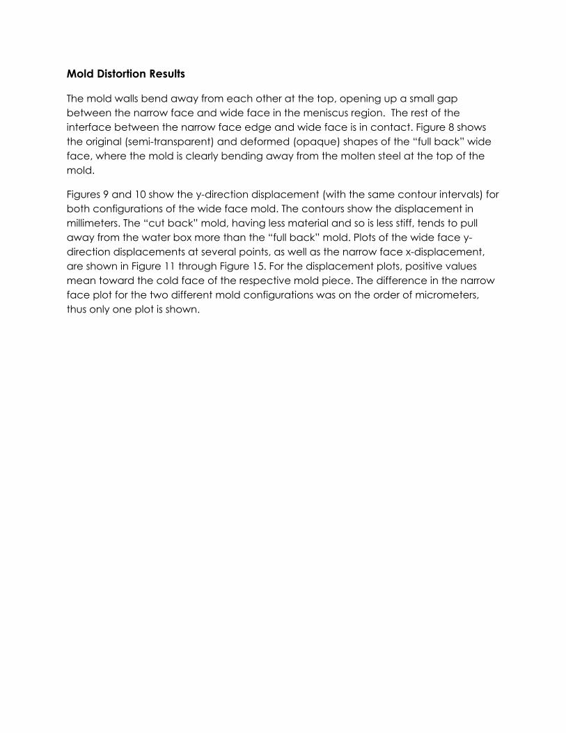
Mold Distortion Results

The mold walls bend away from each other at the top, opening up a small gap between the narrow face and wide face in the meniscus region. The rest of the interface between the narrow face edge and wide face is in contact. Figure 8 shows the original (semi-transparent) and deformed (opaque) shapes of the “full back” wide face, where the mold is clearly bending away from the molten steel at the top of the mold.

Figures 9 and 10 show the y-direction displacement (with the same contour intervals) for both configurations of the wide face mold. The contours show the displacement in millimeters. The “cut back” mold, having less material and so is less stiff, tends to pull away from the water box more than the “full back” mold. Plots of the wide face y-direction displacements at several points, as well as the narrow face x-displacement, are shown in Figure 11 through Figure 15. For the displacement plots, positive values mean toward the cold face of the respective mold piece. The difference in the narrow face plot for the two different mold configurations was on the order of micrometers, thus only one plot is shown.

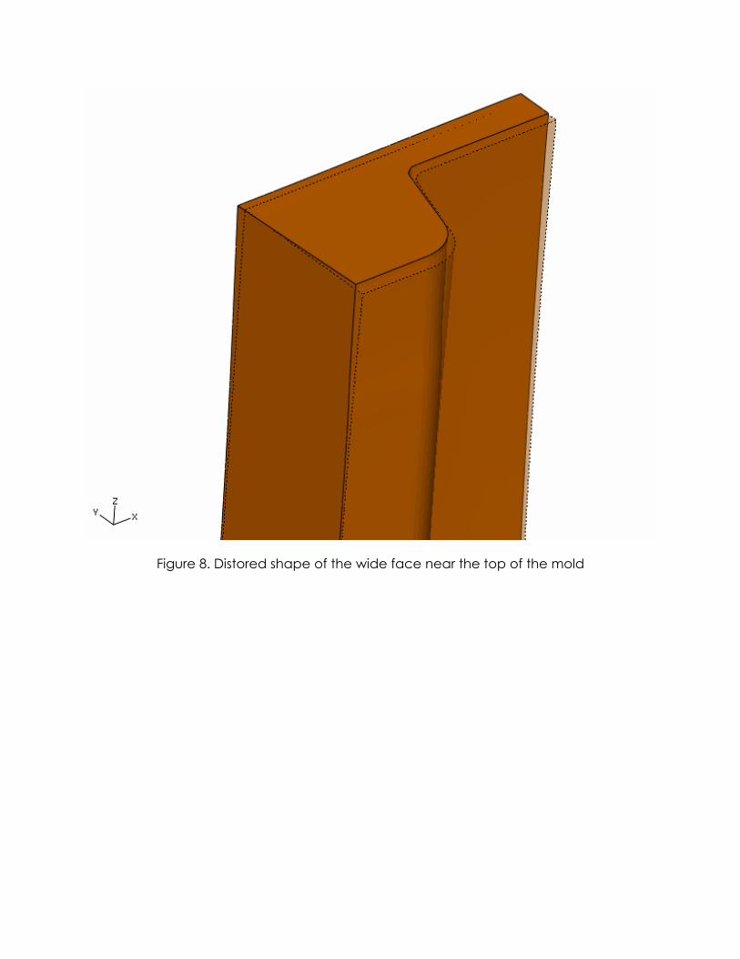
Figure 8. Distored shape of the wide face near the top of the mold

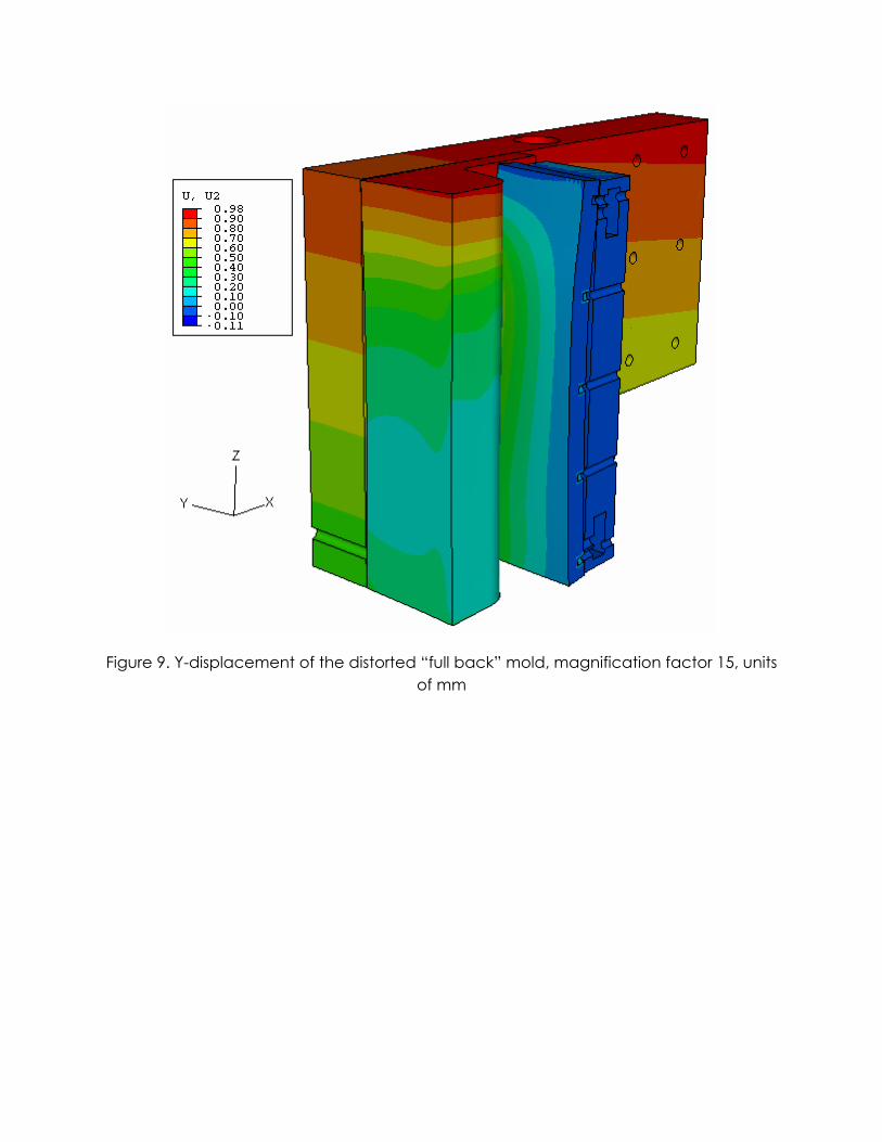
Figure 9. Y-displacement of the distorted “full back” mold, magnification factor 15, units of mm

Figure 10. Y-displacement of the distorted “cut back” mold, magnification factor 15, units of mm

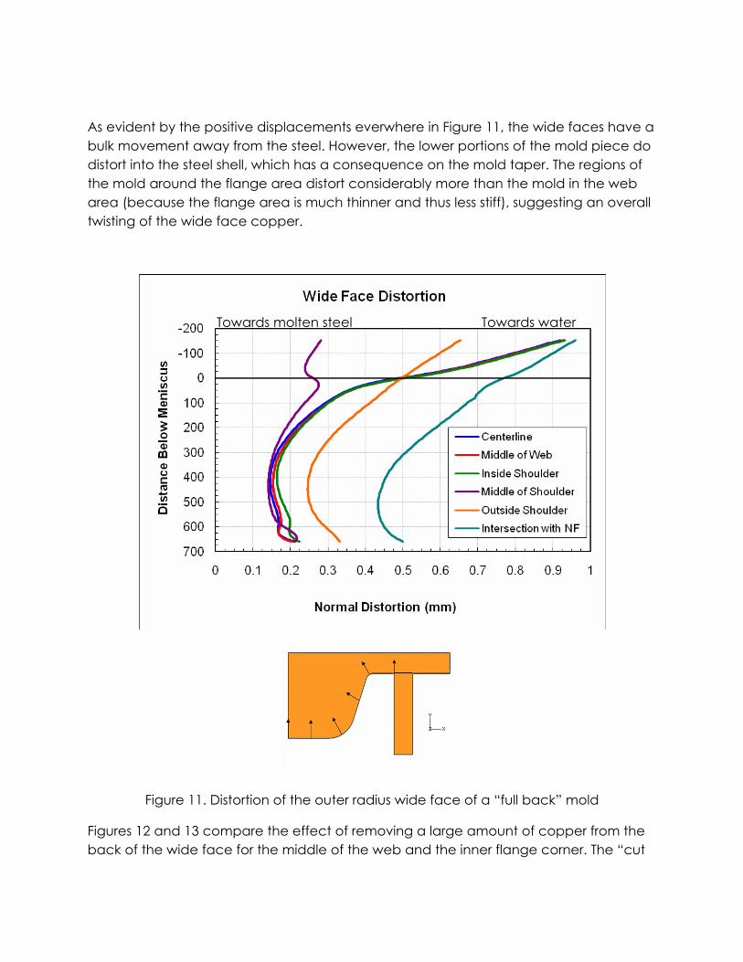
As evident by the positive displacements everwhere in Figure 11, the wide faces have a bulk movement away from the steel. However, the lower portions of the mold piece do distort into the steel shell, which has a consequence on the mold taper. The regions of the mold around the flange area distort considerably more than the mold in the web area (because the flange area is much thinner and thus less stiff), suggesting an overall twisting of the wide face copper.

Figure 11. Distortion of the outer radius wide face of a “full back” mold

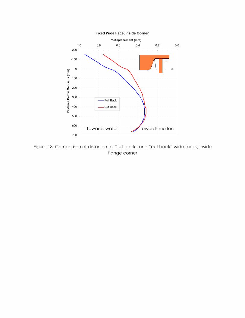
Figures 12 and 13 compare the effect of removing a large amount of copper from the back of the wide face for the middle of the web and the inner flange corner. The “cut

Towards water Towards molten steel

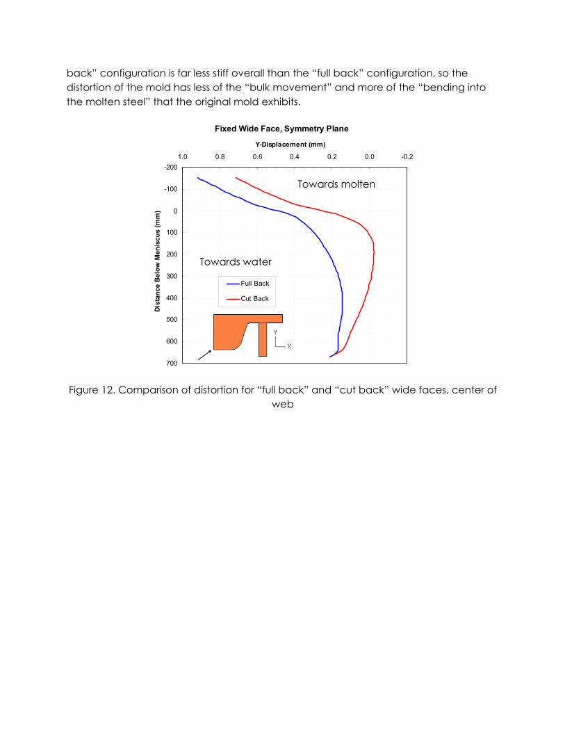
back” configuration is far less stiff overall than the “full back” configuration, so the distortion of the mold has less of the “bulk movement” and more of the “bending into the molten steel” that the original mold exhibits.

Fixed Wide Face, Symmetry Plane

-200

-100

0

100

200

300

400

500

600

700

-0.20.00.20.40.60.81.0

Y-Displacement (mm)

Dist

ance

Bel

ow M

enis

cus

(mm

)

Full Back

Cut Back

Figure 12. Comparison of distortion for “full back” and “cut back” wide faces, center of web

Towards water

Towards molten

Fixed Wide Face, Inside Corner

-200

-100

0

100

200

300

400

500

600

700

0.00.20.40.60.81.0

Y-Displacement (mm)

Dist

ance

Bel

ow M

enis

cus

(mm

)

Full Back

Cut Back

Figure 13. Comparison of distortion for “full back” and “cut back” wide faces, inside flange corner

Towards water Towards molten

Narrow Face Distortion

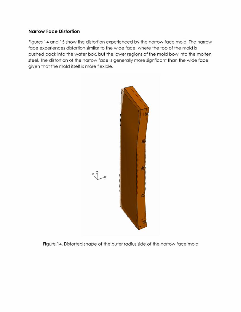
Figures 14 and 15 show the distortion experienced by the narrow face mold. The narrow face experiences distortion similar to the wide face, where the top of the mold is pushed back into the water box, but the lower regions of the mold bow into the molten steel. The distortion of the narrow face is generally more signficant than the wide face given that the mold itself is more flexible.

Figure 14. Distorted shape of the outer radius side of the narrow face mold

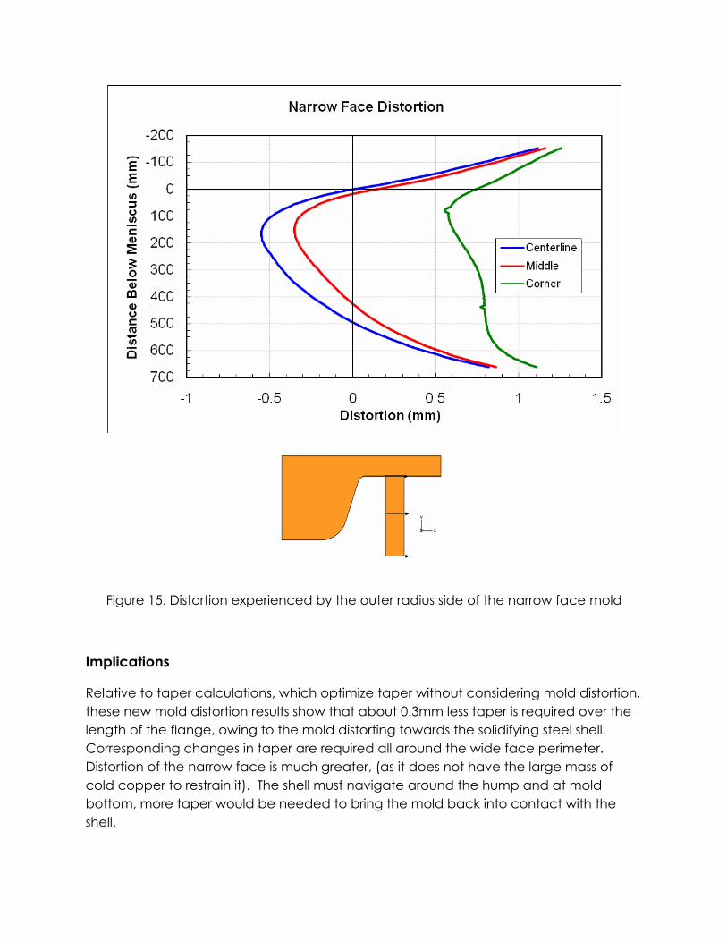
Figure 15. Distortion experienced by the outer radius side of the narrow face mold

Implications

Relative to taper calculations, which optimize taper without considering mold distortion, these new mold distortion results show that about 0.3mm less taper is required over the length of the flange, owing to the mold distorting towards the solidifying steel shell. Corresponding changes in taper are required all around the wide face perimeter. Distortion of the narrow face is much greater, (as it does not have the large mass of cold copper to restrain it). The shell must navigate around the hump and at mold bottom, more taper would be needed to bring the mold back into contact with the shell.

Further work is needed with the shell solidification model to optimize taper based on these results.