molcas 7: the next generation
TRANSCRIPT
Software News and Update
MOLCAS 7: The Next Generation
FRANCESCO AQUILANTE,1 LUCA DE VICO,2 NICOLAS FERRÉ,3 GIOVANNI GHIGO,4 PER-ÅKE MALMQVIST,5
PAVEL NEOGRÁDY,6 THOMAS BONDO PEDERSEN,5 MICHAL PITONÁK,6,7 MARKUS REIHER,8 BJÖRN O. ROOS,5
LUIS SERRANO-ANDRÉS,9 MIROSLAV URBAN,6 VALERA VERYAZOV,5 ROLAND LINDH5
1Department of Physical Chemistry, University of Geneva, 30 Quai Ernest Ansermet,CH-1211 Geneva, Switzerland
2Department of Chemistry, University of Copenhagen, Universitetsparken 5,DK-2100 Copenhagen, Denmark
3Chimie Théorique, Universités d’Aix-Marseille I,II,III-CNRS, UMR 6264 LaboratoireChimie Provence, Faculté de Saint-Jérôme Case 521, Av. Esc. Normandie Niemen,
13397 Marseille Cedex 20, France4Dipartimento di Chimica Generale e Chimica Organica, University of Turin,
C.so M. d’Azeglio, 10125 Turin, Italy5Department of Theoretical Chemistry, Chemical Center, P.O. Box 124, S-221 00 Lund, Sweden
6Department of Physical and Theoretical Chemistry, Faculty of Natural Sciences,Comenius University, Mlynska Dolina CH-1, 842 15 Bratislava, Slovak Republic
7Institute of Organic Chemistry and Biochemistry, Academy of Sciences of the Czech Republic andCenter of Biomolecules and Complex Molecular Systems, Flemingovo nám. 2,
166 10 Prague 6, Czech Republic8 Laboratorium für Physikalische Chemie, ETH Zurich, Hönggerberg Campus,
Wolfgang-Pauli-Strasse, 10, CH-8093 Zurich, Switzerland9Departamento de Química Física, Instituto de Ciencia Molecular, Universitat de València, P.O.
Box 22085, ES-46071 Valencia, Spain
Received 12 February 2009; Revised 3 April 2009; Accepted 6 April 2009DOI 10.1002/jcc.21318
Published online 4 June 2009 in Wiley InterScience (www.interscience.wiley.com).
Abstract: Some of the new unique features of the MOLCAS quantum chemistry package version 7 are presentedinthis report. In particular, the Cholesky decomposition method applied to some quantum chemical methods is described.This approach is used both in the context of a straight forward approximation of the two-electron integrals and in thegeneration of so-called auxiliary basis sets. The article describes how the method is implemented for most known wavefunctions models: self-consistent field, density functional theory, 2nd order perturbation theory, complete-active spaceself-consistent field multiconfigurational reference 2nd order perturbation theory, and coupled-cluster methods. The reportfurther elaborates on the implementation of a restricted-active space self-consistent field reference function in conjunctionwith 2nd order perturbation theory. The average atomic natural orbital basis for relativistic calculations, covering the wholeperiodic table, are described and associated unique properties are demonstrated. Furthermore, the use of the arbitrary orderDouglas-Kroll-Hess transformation for one-component relativistic calculations and its implementation are discussed. Thissection especially focuses on the implementation of the so-called picture-change-free atomic orbital property integrals.Moreover, the ElectroStatic Potential Fitted scheme, a version of a quantum mechanics/molecular mechanics hybrid
Correspondence to: R. Lindh; e-mail: [email protected] orV. Veryazov; e-mail: [email protected]/grant sponsor: Swedish Science Research CouncilContract/grant sponsor: ETH Zurich; contract/grant number: ETH grant0-20436-07Contract/grant sponsor: Schweitzer Nationalfonds; contract/ grant number:project 200020-121870
Contract/grant sponsor: Slovak Research and Development Agency; con-tract/grant number: APVV-20-018405Contract/grant sponsor: Ministry of Education of the Czech Republic (Centerfor Biomolecules and Complex Molecular Systems, LC512); contract/grantnumber: Z4 055 0506Contract/grant sponsor: Consolider-Ingenio in Molecular Nanoscience ofthe Spanish MEC/FEDER; contract/grant numbers: CTQ2007-61260 andCSD2007-0010
© 2009 Wiley Periodicals, Inc.
MOLCAS 7: The Next Generation 225
method implemented in MOLCAS, is described and discussed. Finally, the report discusses the use of the MOLCASpackage for advanced studies of photo chemical phenomena and the usefulness of the algorithms for constrained geometryoptimization in MOLCAS in association with such studies.
© 2009 Wiley Periodicals, Inc. J Comput Chem 31: 224–247, 2010
Key words: MOLCAS; ANO-RCC; RASPT2; ESPF; Cholesky decomposition; coupled cluster; Douglas-Kroll-Hess;photo chemistry
Introduction
The origin of the MOLCAS* package can be traced back to thenovel work during the 1970s of the group of Roos1 at the Stock-holm University, Sweden. Together with his students, J. Almöf,P. E. M. Siegbahn, and U. Wahlgren, they developed improvedand novel methods for electron-integral evaluation (Molecule), thedirect configuration interaction technique,2 implemented single,and multiconfigurational reference configuration interaction (SDCIand MRCI),3 developed the single most successful version of themulticonfigurational SCF method, the complete active space SCF(CASSCF) method,4–6 derived new systematic Gaussian basis setfor molecular calculation,7–9 etc. Much of the work was inspired bythe young scientist’s visits to the quantum chemistry group at theIBM Almaden research center in San Jose, headed by E. Clementi.The work of the Stockholm group formed the backbone of the origi-nal version of MOLCAS, which was presented the first time in 1989.This, the first version of MOLCAS, had many similarities with theMolecule-Sweden package, which for many years was the workhorse of the quantum chemistry group at NASA Ames. However,developments during the 1990 and the following decade has madeMOLCAS into a more versatile and user-friendly program packageas compared with the original version, which would only run onthe IBM 3090 computers under the JCL operating system. Notableupgrades were the introduction of the multiconfigurational referencesecond order perturbation theory (CASPT2) approach10–12 and theMulti-State CASPT2 (MS-CASPT2),13 improved two-electron inte-gral evaluation,14, 15 methods for gradient evaluation,16, 17 geometryoptimization,18, 19 frequency calculations,20 extensions to additionalwave function methods, the generalization of the CASSCF to arestricted active space (RASSCF),21, 22 the development of theCASSCF state interaction method (CASSI),23 the introduction ofspin-orbit coupling (RASSI-SO),24 and improvements with respectto single determinant methods, in particular it is worth to mention thework on coupled-cluster theory.25 However, the MOLCAS packagewas for a long time a package which only targeted highly correlatedcalculations of rather small systems, although a DFT option hasfor some time been included. The status of the MOLCAS package,as of 2003, was at that time presented26 and the philosophy andinfrastructure behind the package was documented in a subsequentpublication.27
*MOLCAS has derived its name from two of the modules in the originalversion, the Molecule integral generator of J. Almlöf and the CASSCF mod-ule of B. O. Roos. Neither the Molecule nor the CASSCF module made theirway to the second version of MOLCAS, in which they were replaced withmore general substitutes. http://www.molcas.org
MOLCAS version 7, as compared with earlier versions, consti-tutes a substantial improvement regarding the size of the systemswhich can be handled by the various wave function models, theversatility of the package, the applicability of the implementedmethods to the whole periodic table, improvements with respectto the bottleneck within the CASSCF/CASPT2 paradigm—thesize of the so-called active space—implementation of a quantummechanics/molecular mechanics (QM/MM) model which can inprinciple support any kind of MM force-fields and the applicabil-ity of the package to significant parts of the lower excited statesas, for example, expressed by photochemistry. This report here willpresent these new developments and extensions in a compact andeasy-to-understand way. The purpose of the article, however, isnot to be too detailed, but to summarize the methods and imple-mentation into a single document. It should be mentioned that thenewest version of MOLCAS does not only include these reportednew features. Additional improvements as a simplified user input,a graphical user interface, add-ons, improved tutorials, etc., are notincluded in this report. Furthermore, some of the methods presentedhere relates to parallelization. In that respect it should be notedthat the RASSCF and RASPT2 modules only include paralleliza-tion with respect to the formation of Fock-matrices and transformedtwo-electron repulsion integrals.
Cholesky Decomposition in MOLCAS
Storage and transformation of two-electron integrals from atomicorbital (AO) to molecular orbital (MO) basis have been majorbottlenecks in previous versions of MOLCAS. As of version 7,however, MOLCAS features the Cholesky decomposition (CD)technique28, 29 which substantially reduces the effort involved intwo-electron integral handling.30–32 The CD is also used for gener-ating auxiliary basis sets for the density fitting (DF)/resolution-of-the-identity (RI) technique,33–38 which is available in MOLCAS-7as well.39 The CD-based development in MOLCAS-7 has been pub-lished in a number of research papers39–47 and a review will appearsoon (Pedersen et al., Theor Chem Acc, to be submitted).
Cholesky Decomposition of Two-Electron Integrals
The Cholesky representation of the two-electron integrals in AObasis is given by30, 31
(µν|λσ) ≈M∑
J=1
LJµνLJ
λσ , (1)
Journal of Computational Chemistry DOI 10.1002/jcc
226 Aquilante et al. • Vol. 31, No. 1 • Journal of Computational Chemistry
where we have used Mulliken notation for the integrals and Greekletters to denote AOs. The Cholesky vectors are computed from aresidual matrix in a recursive procedure according to
LJµν = [
�(J−1)[λσ ]J ,[λσ ]J
]−1/2�
(J−1)µν,[λσ ]J
, (2)
where the residual matrix is defined by
�(J)µν,λσ = (µν|λσ) −
J∑K=1
LKµνLK
λσ , (3)
and [λσ ]J is the index of the largest residual diagonal element at the(J − 1)th recursion, i.e., the index of the parent product |λσ) givingrise to the Jth Cholesky vector. We refer to the subset {|[λσ ]J)} ofthe product functions as the Cholesky basis.
A symmetric positive semidefinite matrix,30 the residual matrixsatisfies the Cauchy-Schwarz inequality
∣∣�(J)µν,λσ
∣∣ ≤√
�(J)µν,µν�
(J)λσ ,λσ . (4)
Introducing the decomposition threshold δ ≥ 0 and using
maxµν
(�(M)
µν,µν
) ≤ δ, (5)
as stop criterion for the recursive procedure, we obtain from eq. (4)that the integrals are represented with absolute accuracy δ:
∣∣�(M)µν,λσ
∣∣ ≤ δ. (6)
It should be noted, however, that the subset of the integrals cor-responding to the parent product functions is represented exactly(within machine precision):
�(M)[µν]J ,[λσ ]K
= 0. (7)
This means that the “most important” (as defined by the CDprocedure) integrals are represented exactly and is a fundamentalreason why the CD technique is accurate even with rather largevalues of the decomposition threshold.47
The computational bottleneck of the CD procedure is the calcu-lation of the residual matrix, eq. (3). In an integral-direct approach,31
only those columns that give rise to Cholesky vectors are calculated,meaning that only a fraction (usually 1–5%) of the integral matrixis needed to generate the Cholesky representation. Calculation ofthe residual matrix requires two steps in each recursion: calculationof the integral column (µν|[λσ ]J) and subtraction of contributionsfrom previous Cholesky vectors. Which of the two steps is the moreexpensive depends on the nature of the basis functions (number ofprimitive Gaussians, angular quantum number) and on the valuechosen for the decomposition threshold. For basis sets with a largenumber of primitive Gaussians and with high angular quantum num-bers, the integral calculation step tends to dominate, whereas the
subtraction step usually dominates for smaller basis sets. The sub-traction shows a computational complexity of NpM2 where Np is thenumber of significant product functions |µν), as estimated using theCauchy-Schwarz inequality. Decreasing the decomposition thresh-old (increasing accuracy) therefore leads to a computational penaltyscaling quadratically with the increase of the number of Choleskyvectors. The Cholesky vectors are stored in a buffer in memory.When the buffer is full, the vectors must be read back into memoryfrom disk, creating a potential I/O bottleneck which can be reducedor avoided by increasing memory.
Damped prescreening based on eq. (4) is employed in each recur-sion. Specifically, a product function |µν) is removed when thefollowing inequality is satisfied:
s√
�(J)µν,µν�
(J)max ≤ δ, (8)
where �(J)max is the largest residual diagonal and s ≥ 1 is the damp-
ing. The latter is chosen according to s ≈ 109δ for decompositionthresholds above 10−8 and s = 1.0 for lower thresholds. As a conse-quence of the damped prescreening, the dimension of the Choleskyvectors is decreased in each recursion and even integrals with val-ues below the decomposition threshold have a nonzero Choleskyrepresentation. As noted in ref. 31, the damping serves as a safe-guard against rounding errors that may render the decompositionnumerically unstable.
SEWARD, the integral program of MOLCAS, is atomic shell-driven.14 As a consequence, individual integral columns cannot beefficiently calculated, and we compute instead the entire set of inte-gral columns (µν|AB) where AB denotes the shell-pair to which thelargest residual diagonal element belongs. New Cholesky vectorsare then generated from this shell-pair as long as the largest residualdiagonal element within this shell-pair is at least a “span factor”times the globally largest residual diagonal element. The defaultspan factor in MOLCAS is 0.01, meaning that the CD recursionscontinue within the calculated shell-pair until the globally largestdiagonal is more than 100 times larger. This shell-driven integral-direct approach has two consequences: first, the total number ofCholesky vectors depends weakly on the chosen span factor and,second, shell-pair integral columns may be calculated more thanonce. The latter is, of course, particularly important for large basissets where the integral calculations are expensive.
To reduce the cost of integral recalculations, the decompositionis performed in two steps. In the first step, all rows and columnsof the residual matrix corresponding to diagonal elements smallerthan the decomposition threshold are discarded in each recursion. Inother words, all diagonals that cannot give rise to a Cholesky vectorare removed, minimizing the dimension of the residual matrix tobe calculated in each recursion. The computational cost of integralrecalculations and Cholesky vector I/O is thus minimized due to thelow dimension of the residual matrix. The essential output from thefirst step is the Cholesky basis, i.e., the mapping from the vectorindex J to the parent product index λσ . Given this mapping, thefull-dimension Cholesky vectors are calculated in the second stepaccording to eq. (2) with the prescreening of eq. (8). Integral recal-culations are thus avoided and Cholesky vector I/O minimized inthe second step.
Journal of Computational Chemistry DOI 10.1002/jcc
MOLCAS 7: The Next Generation 227
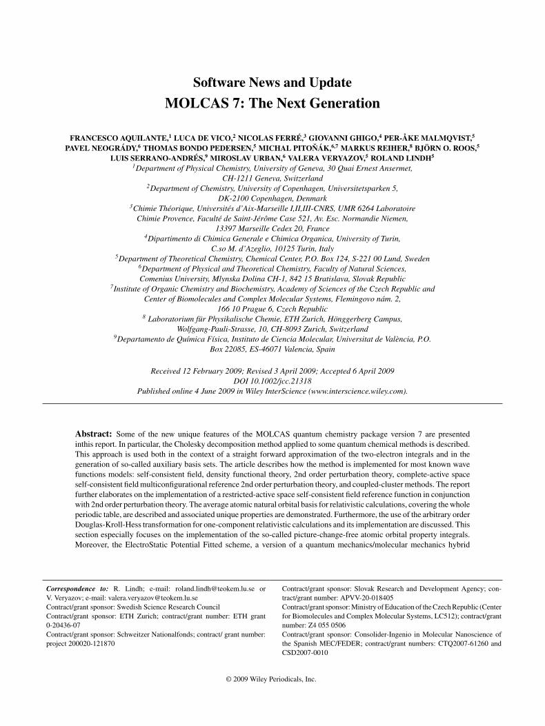
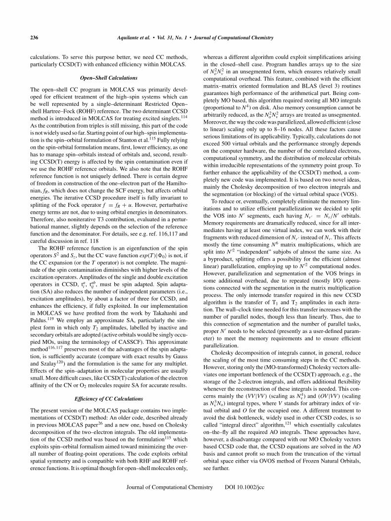
Figure 1. The ratio M/N as a function of decomposition threshold forANO-L-PVXZ (X = D, Q) AO basis sets. M is the number of Choleskyvectors and N the number of AO basis functions. The ratio is calculatedas an average for the molecules of Set I (a subset of the G2-97 test set)of ref. 47.
In a parallel execution, the rows of the residual matrix are (stat-ically) distributed among the processes. In a given recursion, eachprocess calculates the corresponding rows of the integral matrix andperforms the subtraction of previous Cholesky vectors according toeq. (3). This requires that the Cholesky vector elements correspond-ing to the selected integral columns [LK
λσ in eq. (3)] are broadcastfrom the process holding them. This design ensures that the memoryrequirement per process is minimized and that Cholesky vector I/Ocan be avoided by increasing the number of compute nodes (increas-ing available memory). Once the CD has completed, the Choleskyvectors are stored on disk for later use. For the disk storage, how-ever, complete Cholesky vectors are distributed among the nodes,i.e., L1 is stored on node 0, L2 on node 1, L3 on node 2, and so on.
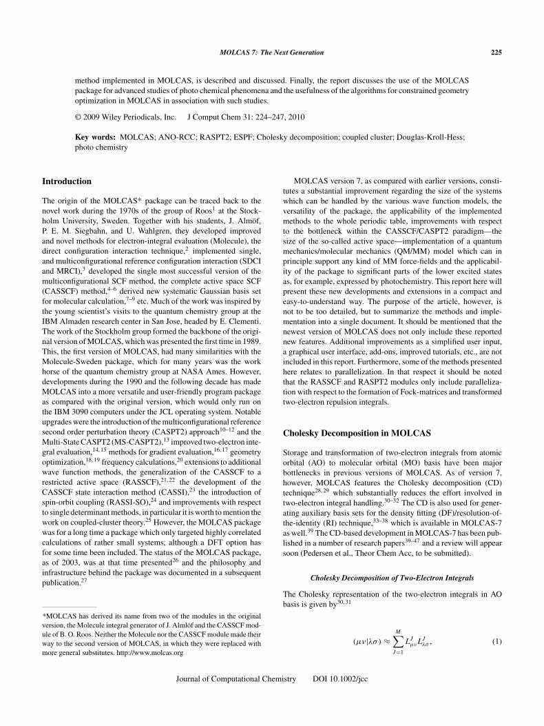
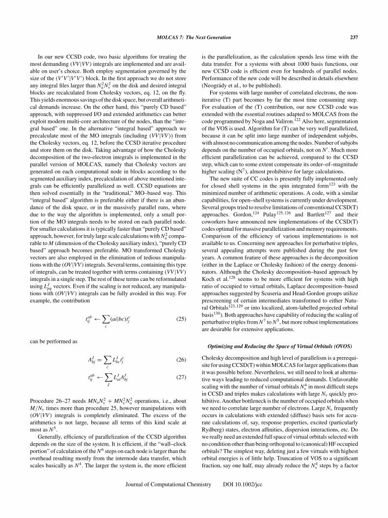
The Cholesky basis generally contains both one- and two-centerproduct functions. We have implemented the so-called one-centerCD (1C-CD)39 in which no two-center functions are allowed to enterthe Cholesky basis. As shown in ref. 47, the two-center functionsare needed for high accuracy (low decomposition threshold), in par-ticular with lower-quality AO basis sets. As can be seen in Figure 1,the computational advantage (lower M) of 1C-CD increases withdecomposition threshold and is particularly pronounced for thedouble-ζ (lower quality) basis set. The scaling of M with systemsize is linear, as seen from Figure 2. As the scaling of the number ofAO basis functions, N , is trivially linear, this implies that the ratioM/N is constant, as also shown in Figure 2.
Analytic gradients of the integrals have been defined for theCholesky representation.43 At the moment, however, analytic gra-dients can only be calculated in conjunction with nonhybrid DFTand the 1C-CD option. Numerical gradients can be calculated withall CD-based options, of course.
Quantum Chemistry with Cholesky Decomposition
Having performed the CD of the two-electron integral matrix, theresulting Cholesky vectors can be used for HF, DFT, MP2, scaledopposite spin (SOS) MP2, RASSCF, CASSCF, RASSI, CASPT2,
and CCSD(T) calculations. The Cholesky vectors are used directlyto construct Fock matrices and two-electron integrals in MO basis.
Inactive and active Fock matrices are calculated in AO basisaccording to41, 44
Fµν =∑
J
LJµν
∑λσ
LJλσ Dλσ − 1
2
∑J
∑k
LJµkLJ
νk , (9)
where k runs over either inactive or active orbital indices and D isthe corresponding density matrix. The half-transformed Choleskyvectors are calculated according to
LJµk =
∑ν
LJµνCνk , (10)
where C is the MO coefficient matrix. Although the Coulombpart of eq. (9) scales quadratically with system size, the exchangepart, including the transformation of eq. (10), scales cubically. Wehave therefore developed the “Local Exchange” (LK)39 algorithm,which reduces the scaling to quadratic by using localized MOs andprescreening based on rigorous upper bounds. To reduce the com-putational cost of orbital localization, MOLCAS uses the so-calledCholesky MOs obtained by performing a CD of the density matrix.40
Two-electron integrals in MO basis are calculated from trans-formed Cholesky vectors according to
(pq|rs) =∑
J
LJpqLJ
rs, (11)
where p, q, r, s denote MOs, and
LJpq =
∑µ
Cµp
∑ν
LJµνCνq. (12)
Figure 2. The number of Cholesky vectors M, number of AO basisfunctions N , and the ratio M/N (multiplied by 1000) as functions ofthe number of glycine units in linear glycine chains. The basis set iscc-pVDZ and the decomposition threshold is δ = 10−4.
Journal of Computational Chemistry DOI 10.1002/jcc
228 Aquilante et al. • Vol. 31, No. 1 • Journal of Computational Chemistry
Only those integrals that are needed by a given methodare computed according to eq. (11), thus significantly reducingthe computational cost compared with conventional calculations.MOLCAS generates the (ai|bj) integrals on-the-fly while calculat-ing the MP2 energy correction [i, j refer to occupied orbitals, a, b tovirtual orbitals], whereas the MO integrals needed by the CASPT2method are generated, written to disk, and read back into mem-ory in the CD-CASPT2 implementation. Although the CD-MP2code is significantly faster than the conventional implementation,the CD-CASPT2 code mainly reduces the wall-time of the cal-culation due to decreased I/O.45 Both CD-MP2 and CD-CASPT2can be applied to substantially larger systems than the conventionalprograms, as exemplified in refs. 45, 48, 49. As described in moredetail below, the new CD-based implementation of coupled clustertheory in MOLCAS can use Cholesky vectors in two ways. Either theMO integrals are calculated and stored on disk prior to the iterativeCCSD procedure or they are calculated on-the-fly.
Density Fitting and Auxiliary Basis Sets fromCholesky Decompositions
The DF approximation is given by33–38
(µν|λσ) ≈∑PQ
(µν|P)G−1PQ(λσ |Q), (13)
where P, Q refer to auxiliary basis functions, G−1PQ = (G−1)PQ, and
GPQ = (P|Q). As the G matrix is symmetric positive definite, itsinverse can be Cholesky decomposed, i.e.
G−1PQ =
∑K
ZKP ZK
Q . (14)
Combining eq. (14) and eq. (13), and introducing the DF vectors
RKµν =
∑P
(µν|P)ZKP , (15)
we obtain the expression
(µν|λσ) ≈∑
K
RKµνRK
λσ , (16)
which has the same form as the Cholesky representation, eq. (1).The DF vectors are generated by SEWARD and stored in the samemanner as Cholesky vectors. Thus, the MOLCAS modules usingCholesky vectors can also be executed using DF vectors.
MOLCAS generates auxiliary basis sets on-the-fly, as describedin refs. 39, 46 and benchmarked along with CD in ref. 47. Twotypes of CD-based auxiliary basis sets are available in MOLCAS:the atomic CD (aCD)39 and the atomic compact CD (acCD).46 TheaCD set is generated by a decomposition of the atomic two-electronintegral matrix, identifying the resulting Cholesky basis (see above)as the auxiliary functions for the given atom type and basis set.To make the integral evaluation more efficient, “missing” angular
components of the product functions of the Cholesky basis areadded to complete the shell structure of the auxiliary basis (seerefs. 39, 46 for further details). The acCD set is generated from thecorresponding aCD set by removing linear dependence in the prim-itive Gaussian product basis by performing a CD of an “angularfree” integral matrix, as described in ref. 46. The number of aux-iliary functions is thus the same for aCD and acCD sets, but thenumber of primitive Gaussians is reduced in the latter, making thegeneration of DF vectors faster for large basis sets. The accuraciesof the aCD and acCD sets are almost identical, though.46, 47
As the aCD and acCD auxiliary basis sets are constructed by CDof the atomic integral matrix, they may be used with any AO basisset. Moreover, they may be used in conjunction with any quantumchemical method. In short, the aCD and acCD auxiliary basis sets areunbiased. Constructed on-the-fly, the aCD and acCD basis sets aregenerated automatically in MOLCAS, requiring no other user-inputthan the decomposition threshold (if the default is not sufficient).Care must be exercised for small AO basis sets on hydrogen andhelium atoms; however, in the absence of polarization functions inthe AO basis set, the aCD and acCD sets solely contain s-functionson hydrogen and helium atoms, leading to unusually large errors intotal energies.46
ANO-RCC: A Basis Set for the Entire Periodic Table
MOLCAS is a program system that allows calculations in the rela-tivistic regime. As described earlier, the Douglas-Kroll-Hess (DKH)transformation of the Dirac Hamiltonian is used in a two-componentformulation of the relativistic wave function. The scalar part of theDKH Hamiltonian replaces the one-electron nonrelativistic Hamil-tonian and all methods that are used in nonrelativistic calculationswill automatically include these effects. However, the basis sets thatare normally used cannot be transferred to the relativistic regime.The contraction of the inner shells are different and this will affectthe structure also for the valence orbitals. It is therefore necessary todevelop specific basis sets where the DKH Hamiltonian is includedwhen the basis set is constructed.
Here we have developed such basis sets for the atoms H-Cmbased on the concept of density averaged Atomic Natural Orbitals(ANOs). Such basis sets have been available in MOLCAS in the non-relativistic regime for the atoms H-Zn, as the ANO-L and ANO-Sbasis sets.50–53 The new basis sets have been labelled ANO-RCC toindicate that they are relativistic (R) and that semicore electrons havebeen included in the correlation treatment (CC). The densities usedfor the construction of the ANOs have been obtained from multicon-figurational wave functions have been used (CASSCF) with the mostimportant orbitals in the active space, where dynamic correlation istreated using second order perturbation theory (CASPT2).10, 11, 54
This approach was used because it is general and can be applied toall electronic states independent of their spin and space symmetry.The basis sets have been generated without the inclusion of spin-orbit coupling which we do not believe to be very important for theshape of the orbitals (with the exception of the heavier main groupelements, where the present approach will not work well anyway).The ANO-RCC basis sets have been published in a series of papersduring the years 2003–2008.55–59
Journal of Computational Chemistry DOI 10.1002/jcc
MOLCAS 7: The Next Generation 229
Table 1. Size of the Primitive Basis Sets and the Contraction Range.
Atoms Primitive Max # of ANOs Atoms Primitive Max # of ANOs
H 8s4p3d1f 6s4p3d1f Rb–Sr 23s19p11d4f 10s10p5d4fHe 9s4p3d2f 7s4p3d2f Y–Cd 21s18p13d6f4g2h 10s9p8d5f4g2hLi–Be 14s9p4d3f1g 8s7p4d2f1g In–Xe 22s19p13d5f3g 10s9p8d5f3gBe–Ne 14s9p4d3f1g 8s7p4d3f2g Cs–Ba 26s22p15d4f 12s10p8d4fNa 17s12p5d4f 9s8p5d2f La 24s21p15d5f3g 11s10p8d5f3gMg 17s12p6d2f 9s8p6d2f Ce–Lu 25s22p15d11f4g2h 12s11p8d7f4g2hAl 17s12p5d3f 9s9p5d3f Hf–Au 24s21p15d11f4g2h 11s10p8d6f4g2hSi–Ar 17s12p5d4f2g 8s7p5d4f2g Hg 25s22p16d12f4g2h 10s10p9d6f4g2hK 21s16p5d4f 10s9p5d3f Tl–Rn 25s22p16d12f4g 11s10p9d6f4gCa 20s16p6d4f 10s9p6d4f Fr–Ra 28s25p17d12f 12s11p8d5fSc–Zn 21s15p10d6f4g2h 10s9p8d6f4g2h Ac–Pa 27s24p18d14f6g3h 13s11p10d8f6g3hGa–Kr 20s17p11d5f2g 9s8p6d4f2g U–Cm 26s23p17d13f5g3h 12s10p9d7f5g3h
The Average Densities
The primitive Gaussian functions used to construct the basis sets arepresented in Table 1. For atoms up to Zn the ANO-L primitives wereused. The primitives for the other atoms were based on the Faegriprimitive sets.60 They were extended with more diffuse functions inan even-tempered way. Higher angular momentum functions wereadded and exponents were optimized for the ground state atoms (atthe CASPT2 level of theory) using an even-tempered extension witha ratio of 0.4.
The construction of the ANOs is based on an average densitymatrix. Calculations with the primitive basis set were performed for:each atom in its ground state, in one excited state, for the positiveion, and for most atoms also the negative atom. Polarization effectswere included by calculations on the ground state atom in an electricfield. For the main group elements calculations were instead madefor the diatomic molecule. More details about the selected electronicstates can be found in the original articles.55–59 An average densitymatrix was constructed as:
ρav =∑
i
ωiρi, (17)
where ρi are the density matrices obtained from the differentCASPT2 wave functions. Usually, the same weight was used forall states included in the averaging. The average density matrix isdiagonalized and ANOs with occupation numbers larger than about10−6 define maximum size of the basis set. For more details, werefer to the basis set library in the MOLCAS package.
Atomic Ionization Energies, Electron Affinities, and Polarizabilities
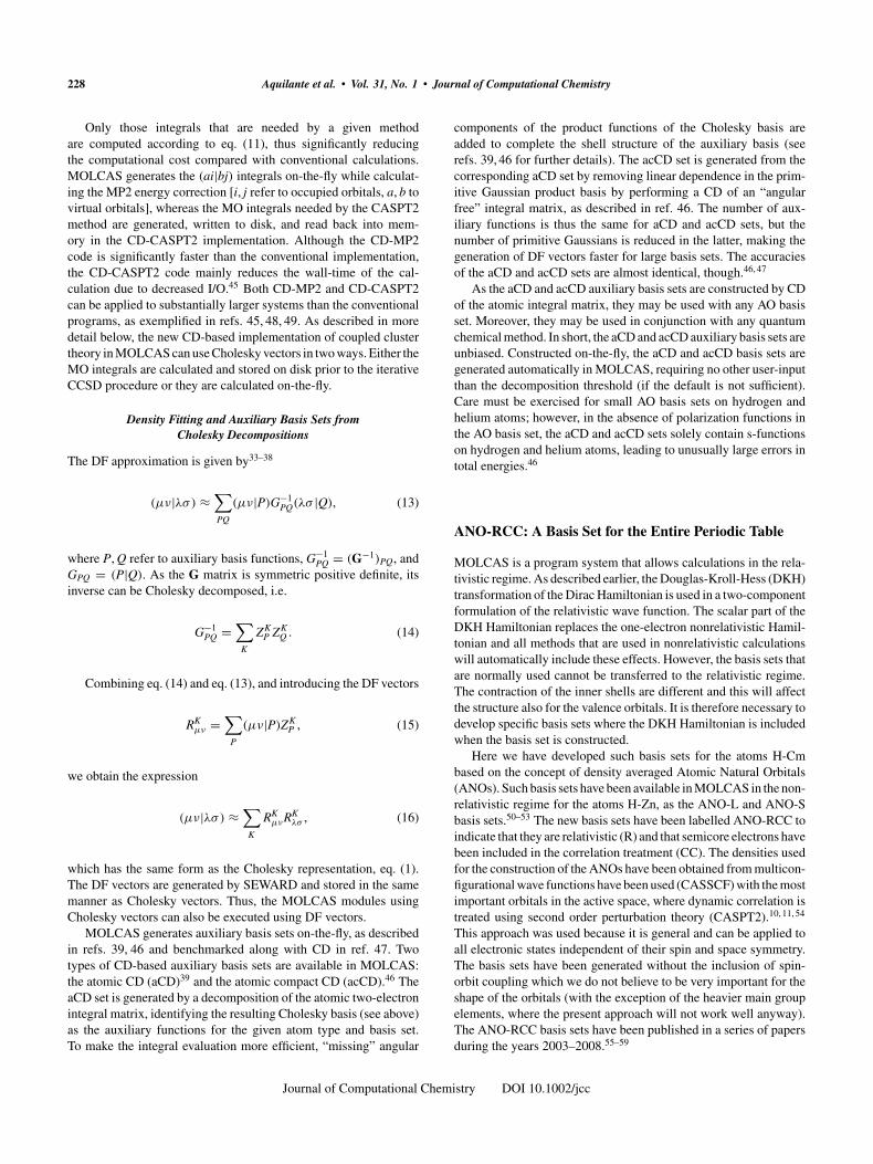
As examples of results that have been obtained during the construc-tion of the basis set we present below the ionization energies(IEs)of all atoms in the range H-Cm, selected electron affinities, andpolarizabilities for spherical atoms. The IEs are shown in Figure 3.Calculations have been performed with the largest basis set butalmost identical results are obtained at the VQZP level. TheseCASPT2 results have an RMS error of 0.15 eV and a maximumerror of 0.28 eV (for the Tc atom). The errors are mainly due to the
CASPT2 approximation and to a lesser extent to limitations in thebasis set.
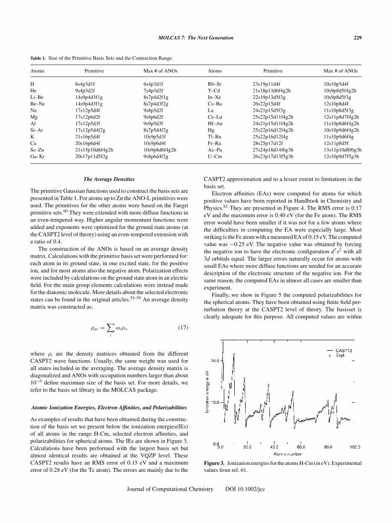
Electron affinities (EAs) were computed for atoms for whichpositive values have been reported in Handbook in Chemistry andPhysics.62 They are presented in Figure 4. The RMS error is 0.17eV and the maximum error is 0.40 eV (for the Fe atom). The RMSerror would have been smaller if it was not for a few atoms wherethe difficulties in computing the EA were especially large. Moststriking is the Fe atom with a measured EA of 0.15 eV. The computedvalue was −0.25 eV. The negative value was obtained by forcingthe negative ion to have the electronic configuration d7s2 with all3d orbitals equal. The larger errors naturally occur for atoms withsmall EAs where more diffuse functions are needed for an accuratedescription of the electronic structure of the negative ion. For thesame reason, the computed EAs in almost all cases are smaller thanexperiment.
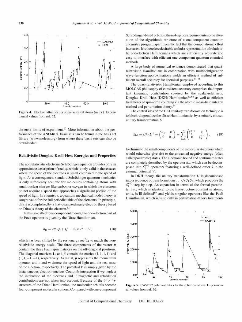
Finally, we show in Figure 5 the computed polarizabilities forthe spherical atoms. They have been obtained using finite field per-turbation theory at the CASPT2 level of theory. The basisset isclearly adequate for this purpose. All computed values are within
Figure 3. Ionization energies for the atoms H-Cm (in eV). Experimentalvalues from ref. 61.
Journal of Computational Chemistry DOI 10.1002/jcc
230 Aquilante et al. • Vol. 31, No. 1 • Journal of Computational Chemistry
Figure 4. Electron affinities for some selected atoms (in eV). Experi-mental values from ref. 62.
the error limits of experiment.62 More information about the per-formance of the ANO-RCC basis sets can be found in the basis setlibrary (www.molcas.org) from where these basis sets can also bedownloaded.
Relativistic Douglas-Kroll-Hess Energies and Properties
The nonrelativistic electronic Schrödinger equation provides only anapproximate description of reality, which is only valid in those caseswhere the speed of the electrons is small compared to the speed oflight. As a consequence, standard Schrödinger quantum mechanicsis only sufficiently accurate for molecules containing atoms withsmall nuclear charges like carbon or oxygen in which the electronsdo not acquire a speed that approaches a significant portion of thespeed of light. In chemistry, a quantum mechanical model theory issought valid for the full periodic table of the elements. In principle,this is accomplished by a first-quantized many-electron theory basedon Dirac’s theory of the electron.63
In this so-called four-component theory, the one-electron part ofthe Fock operator is given by the Dirac Hamiltonian,
hD = cα · p + (β − 14)mc2 + V , (18)
which has been shifted by the rest energy mc214 to match the non-relativistic energy scale. The three components of the vector α
contain the three Pauli spin matrices on the off-diagonal positions.The diagonal matrices 14 and β contain the entries (1, 1, 1, 1) and(1, 1, −1, −1), respectively. As usual, p represents the momentumoperator and c and m denote the speed of light and the rest massof the electron, respectively. The potential V is simply given by theinstantaneous electron–nucleus Coulomb interaction if we neglectthe interaction of the electrons and if magnetic and retardationcontributions are not taken into account. Because of the (4 × 4)-structure of the Dirac Hamiltonian, the molecular orbitals becomefour-component molecular spinors. Compared with one-component
Schrödinger-based orbitals, these 4-spinors require quite some alter-ation of the algorithmic structure of a one-component quantumchemistry program apart from the fact that the computational effortincreases. It is therefore desirable to find a representation of relativis-tic one-electron Hamiltonians which are sufficiently accurate andeasy to interface with efficient one-component quantum chemicalmethods.
A large body of numerical evidence demonstrated that quasi-relativistic Hamiltonians in combination with multiconfigurationwave-function approximations yields an efficient method of suf-ficient overall accuracy for chemical purposes.64–66
The quasi-relativistic Hamiltonian employed according to thisMOLCAS philosophy of consistent accuracy comprises the impor-tant kinematic contribution covered by the scalar-relativisticDouglas–Kroll–Hess (DKH) Hamiltonian67, 68 as well as efficienttreatments of spin–orbit coupling via the atomic mean-field integralmethod and perturbation theory.24
The central idea of the DKH unitary transformation technique isto block-diagonalize the Dirac Hamiltonian hD by a suitably chosenunitary transformation U
hbd = UhDU† =(
h+ 00 h−
)=
∞∑k=0
(E (+)
k 00 E (−)
k
), (19)
to eliminate the small components of the molecular 4-spinors whichwould otherwise give rise to the unwanted negative-energy (oftencalled positronic) states. The electronic bound and continuum statesare completely described by the operator h+, which can be decom-posed into E (+)
k operators featuring a well-defined order k in theexternal potential V .
In DKH theory, the unitary transformation U is decomposedinto a sequence of transformations . . . U2U1U0, which produces theE (+)
k step by step. An expansion in terms of the formal parame-ter 1/c, which is identical to the fine-structure constant in atomicunits, is ill-defined69 and yields singular operators like the PauliHamiltonian, which is valid only in perturbation-theory treatments
Figure 5. CASPT2 polarizabilities for the spherical atoms. Experimen-tal values from ref. 62.
Journal of Computational Chemistry DOI 10.1002/jcc
MOLCAS 7: The Next Generation 231
of relativistic effects. The expansion of hbd, using the external poten-tial V as perturbation parameter, does not give singular operators andcan be used variationally.69 The well-known relativistic terms of thePauli Hamiltonian, like the mass–velocity and Darwin operators, arerecovered from the DKH Hamiltonian after 1/c expansion. Hence,the variationally stable DKH Hamiltonians are an ideal substitutefor the Pauli Hamiltonian and its ingredients, which are now onlyof historical importance.
Except for the first unitary transformation U0, which must bechosen to be the free-particle Foldy–Wouthuysen transformation,69
each unitary transformation Ui can be parameterized in terms ofan anti-Hermitian operator to be chosen in such a way as to elim-inate the off-diagonal coupling terms in the Dirac Hamiltonian.This parameterization can be written in terms of a Taylor seriesexpansion in the most general fashion.70 In actual calculations, aset of coefficients needs to be chosen for this expansion under thecondition that unitarity is still preserved. Up to fourth order in V ,the resulting Hamiltonians are independent of this choice, whereashigher-order Hamiltonians are affected by the choice of parameters.This parameter dependence is, however, negligible71 and vanishes,of course, at infinite order. The arbitrary-order DKH method72 hasbeen implemented in its scalar-relativistic one-electron variant in theMOLCAS program package. A conceptual review of the method canbe found in ref. 73. Five different parameterizations are available inMOLCAS, namely, the optimum, the square-root, the Cayley, theMcWeeny, and the exponential parameterizations.
The unitary transformation technique that is at the heart of DKHtheory requires not only the Hamiltonian to be unitary-transformedbut any operator o. For a sum of one-electron operators this reads
〈o〉 =∑
ij
γij⟨ψDKH
i
∣∣(UoU†)∣∣ψDKHj
⟩, (20)
where ψDKHi denotes the DKH orbitals and γij is a generalized
occupation number (i.e., an element of the first-order densitymatrix to be more precise). If this change of picture is not consis-tently considered, numerical artifacts appear in molecular propertycalculations that are called picture-change errors.74, 75 These arti-facts can be reduced to any desirable order in DKH theory76
and an arbitrary-order algorithm77 has been implemented into theMOLCAS program package.78
It is an interesting feature of magnetic-field-free scalar-relativistic one-electron DKH theory that the resulting DKH Hamil-tonian and DKH property operators can be calculated almostsolely from the nonrelativistic integral matrices. Only two addi-tional types of one-electron integral matrices are required, namely,{〈χµ|p ·Vp|χν〉} and {〈χµ|p · op|χν〉}, where χµ and χν are the usualatom-centered Gaussians. The transformation would, however, bemore complicated for magnetic-field-dependent properties and forproperties that require the perturbed wave function.79
Currently, all one-electron electric-field-like molecular propertyintegrals are subject to a DKH transformation if this is switchedon for the one-electron part of the Fock operator. The efficiency ofthe implementation has been demonstrated for electric-field gradi-ents,78 which are most prone to picture-change artifacts comparedwith other electric-field-like properties.77 It is important to notethat for every physical observable the change of picture must be
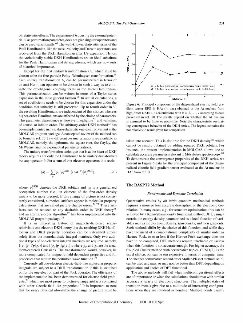
Figure 6. Principal component of the diagonalized electric field gra-dient tensor EFG in HAt (in a.u.) obtained at the At nucleus fromhigh-order DKH(n, n) calculations with n = 2, . . . , 7 according to datapresented in ref. 80 The results depend on whether the At nucleusis assumed to be finite or point-like. Note the characteristic oscillat-ing convergence behavior of the DKH series. The legend contains thenonrelativistic result given for comparison.
taken into account. This is also true for the DKH density,80 whichcannot be simply obtained by adding squared DKH orbitals. Forinstance, the present implementation in MOLCAS allows one tocalculate accurate parameters relevant to Mössbauer spectroscopy.81
To demonstrate the convergence properties of the DKH series, wepresent in Figure 6 data for the principal component of the diago-nalized electric field gradient tensor evaluated at the At nucleus inHAt from ref. 80.
The RASPT2 Method
Nondynamic and Dynamic Correlation
Quantitative results by ab initio quantum mechanical methodsrequires a more or less accurate description of the electronic cor-relation. In many cases, e.g., for structure optimization, this can beachieved by a Kohn-Sham density functional method, DFT, using acorrelation energy density parametrized as a local function of vari-ables such as the electronic density, spin density, and their gradients.Such methods differ by the choice of this function, and while theyhave the merit of a computational complexity of similar order asHartree-Fock, or even less if the Hartree-Fock exchange does nothave to be computed, DFT methods remain unreliable or uselesswhen this function is not accurate enough. For higher accuracy, theCoupled Cluster method with perturbative triples, CCSD(T), is theusual choice, but can be too expensive in terms of computer time.The cheaper perturbative second order Møller-Plesset method, MP2,can be used and may, or may not, be better than DFT, depending onapplication and choice of DFT functional.
The above methods will fail when multiconfigurational effectsare of importance or when the calculations should treat with similaraccuracy a variety of electronic structures. The multiplet states oftransition metals give rise to a multitude of interacting configura-tions when they are involved in bonding. Multiple bonds usually
Journal of Computational Chemistry DOI 10.1002/jcc
232 Aquilante et al. • Vol. 31, No. 1 • Journal of Computational Chemistry
have a component, such as π bonds of most molecules or δ bondsbetween transition metals, which has fractional character. Excitedstates almost always involve several different electronic configura-tions, and for photochemistry the most interesting reaction pathsare often those which pass through regions of swift changes of theadiabatic electronic states.
Traditionally, the correlation effects are classified as dynamic ornondynamic correlation. This classification is by no means strict,nor is it additive. The nondynamic correlation can be stabiliz-ing or destabilizing, depending on the state. It describes a globalelectronic structure that cannot be properly modelled by a single-determinant wave function. The dynamic correlation, on the otherhand, is regarded as resulting mainly from the additional stabiliza-tion by the ability of electrons to simultaneously avoid each other,with small and local effects in the electronic structure. In such aview, the dynamic correlation is always stabilizing.
A method that allows a flexible description of non-dynamiccorrelation is the Complete Active Space Self-Consistent Field(CASSCF) method. It is well suited for dealing with nondynamicnear-degeneracy effects, thereby being able to treat electronicallyexcited molecules, bond dissociation, radicals, transition metal com-pounds, etc., in the same way and with almost uniform accuracy. TheCASSCF method is in principle open-ended, in the sense that a moreaccurate calculation can always be obtained by increasing the num-ber of correlated orbitals. However, the number of configurationscan grow dramatically with such an increase, and for molecules it isnot possible to include more than a fraction of dynamic correlation inthis way (In fact, the CASSCF model often serves as the operationaldefinition of nondynamic correlation). New approaches, wherebyin effect very large CI expansions can be used without the need forexplicit representation of each individual CI coefficient,82–84 offer apossible way to allow larger active spaces, but these are still exper-imental and it is probable that the dynamic correlation must still betreated by separate calculations.
Dynamic correlation effects “on top” of CASSCF, and includingits interplay with the non-dynamic correlation, using, e.g., DFT orCoupled-Cluster methods, is either not technically possible or arestill impractical for large molecular systems, even if there are devel-opment under way in this direction. On the other hand, the MP2method has been extended such that it can compute a perturbativecorrection to CASSCF. This has been implemented as so-calledCASPT2 (CAS Perturbation Theory through second order), and thecombination CASSCF/CASPT2 has turned out to be very successfulfor a large variety of problems. There are also other approaches tosuch corrections. Celani et al.85 made a very large calculation of theCr2 bonding using a combined CI/PT2 approach, and compare withCASPT2 and with another perturbation scheme, called NEVPT2.86
The combination of CASSCF and CASPT2 is almost always nec-essary, as CASSCF alone has very limited ability to handle dynamiccorrelation. Once that the CASSCF has taken care of nondynamiccorrelation, the remaining dynamic correlation is much easier todeal with. It is still large and variable enough that it must usually beincluded, but can be treated perturbatively.
The CASSCF/CASPT2 method is quite complicated in its detailsand implementation, but it has now reached a mature state andhas been shown to yield accurate results for ground and electroni-cally excited states of molecules including atoms across the wholeperiodic table and for arbitrary molecular structures.87–94
CASSCF is in principle a Multiconfiguration Self-ConsistentField (MCSCF) method, which means that it simultaneously opti-mizes both orbitals and CI coefficients for a wave function composedof many configurations. All possible configurations are includedwhich can be formed by distributing a specified number of activeelectrons among a subset of occupied orbitals, the active orbitals,in a way consistent with spin and symmetry of the state. To theuser, this presents a calculation that can be specified similarly as aclosed-shell Hartree-Fock or DFT, in terms of basis set and numberof electrons. It differs, because also the number of orbitals with fulland with fractional occupation, called inactive and active orbitals,respectively, must be specified, together with the spin and pointgroup irrep (symmetry type) of the state(s) to compute. It can, andoften does, compute wave functions and energies for many statessimultaneously. The orbitals are then optimized to give the lowestpossible average energy of these states, whereas the CI expansioncoefficients are optimized to describe the individual states.
Although such calculations are in principle possible for arbi-trary states and molecules, there remain practical limitations. Themost frustrating is the limited size of the active space—the numberof orbitals that must be allowed the freedom of variable occupa-tion. It is possible to correlate a few electrons in a large number oforbitals (like in a Multireference CI calculation, say), but usuallythe number of correlated (active) electrons is comparable with thenumber of active orbitals, and there is then a drastic increase in thesize of the CI expansion with the number of active orbitals. Onemay have to reduce ones ambitions and compromize, and a calcu-lation that is barely possible can still be missing active orbitals ofimportance. Unfortunately, compromizing by omitting even one ortwo orbitals from the preferred active space often results in opti-mization problems of similar kind as for the early selected MCSCFcalculations.
The RASSCF/RASPT2 Concept
When CASSCF/CASPT2 is impractical due to a large numberof configurations, restrictions on the CI expansion space canbe applied. In the RASSCF (Restricted, instead of Complete)method,21, 22 the number of active orbitals, can be much increasedby subdividing the active space into three parts, denoted RAS1,RAS2, and RAS3. The CI space is most easily described as aris-ing from a smaller primary set of configurations by allowing alsosome excitations from this space. In the primary space, the RAS1orbitals are fully occupied, the RAS3 orbitals are unoccupied, andthe RAS2 orbitals play the role of active orbitals for the primary con-figurations, which should be those that are essential for describingthe nondynamic correlation. The full set of configurations are thenthose that differ from the primary set by allowing at most a specifiednumber of electrons to be excited out of the RAS1 space, and at mosta specified number of electrons excited into the RAS3 space. Thefull set of configurations thus described is used in the calculation;there is no difference in treatment of primary and excited configu-rations, and this subdivision is done just to describe the structure ofthe CI space.
This method was implemented from the start in the currentlyused program, but it has been used mostly for CASSCF calcula-tions, which are thus regarded as a special case of RASSCF. Thereason is partly that true RASSCF calculations usually require some
Journal of Computational Chemistry DOI 10.1002/jcc
MOLCAS 7: The Next Generation 233
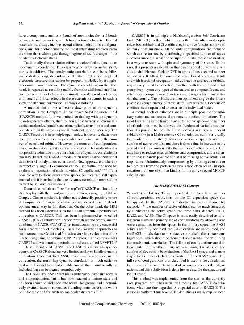
Figure 7. The copper-bis(µ)oxo complex.
experimentation and “hands-on” preparation of starting orbitals toconverge to an acceptable solution, and that convergence can beslow and capricious. The extension of the CASPT2 concept to com-pute perturbative dynamic correlation also from an unperturbedwave function of the RASSCF type is naturally called RASPT2.A first implementation was made by Celani and Werner95 in amultireference configuration interaction, (MRCI) program.
In contrast to CASPT2, there is yet little experience of the moregeneral RASPT2, but it has now been implemented as a modificationof the CASPT2 program used in MOLCAS, and was found useful,e.g., in the study of some copper complexes of biological interest.It has been found that, in order to properly describe the relativeenergetics, a second d-shell with correlating orbitals is necessary.This requires ten active orbitals per transition metal atom, in additionto any further active orbitals needed for excited states and/or bondbreaking. The copper-bis(µ)oxo complex in Figure 7 could not bewell described with less then 32 active orbitals with 28 electrons.A CASSCF wave function would have comprised on the order of1017 determinant functions, but the calculation could be done tosatisfaction using RASSCF/RASPT2.96
Apart from the obvious advantage of allowing a larger number ofactive, i.e., nondynamically correlated orbitals, there are complica-tions that the user should be aware of. While the CASSCF/CASPT2method is now a standard tool for many types of calculations,it is not a “black box” method. This is even more true forthe RASSCF/RASPT2 combination, and a user may need somebackground of technical details.
RASPT2: Technical Issues
At present, a CASPT2 or RASPT2 calculation can be roughlydivided up into three phases: computing a zeroth-order Hamilto-nian for the perturbation expansion; solving the equation systemthat gives the amplitudes describing the perturbation; and finallyusing these to compute energies and other properties of interest.
In principle, CASPT2 and Multi-State CASPT2 solves a set ofequations of the usual Rayleigh-Schrödinger type
(H0 − E0
)∣∣�(1)⟩ = (
H − E0)∣∣�(0)
⟩(21)
∣∣�(1)⟩ =
M∑P=1
cPXP
∣∣�(0)⟩
(22)
where H0 is an approximation to H , which is a second-quantizationrepresentation of the true Hamiltonian. �(0) is the unperturbed wave
function, which is a RASSCF wave function. �(1) is the first-orderwave function, which is parametrized in terms of a set of excitationoperators, {XP}, acting on �(0), and E0 is the energy expectationvalue of the RASSCF wave function. The right-hand side is con-tained in the so-called interacting space, which is spanned by allwave functions generated by the terms of the Hamiltonian whenacting on �(0), orthogonal to �(0) itself. Identically the same spaceis spanned by the terms comprising the expansion of �(1), whichmeans that the equation can be solved exactly provided that theinteraction space is a stable space for the action of H0 − E0.
This parametrization is very much smaller than an equivalentexpansion in terms of individual Slater determinants, because eachterm is comprised of a number of contributing determinants gen-erated from �0. As a typical application, consider a CASSCFcalculation with 12 active electrons in nA = 12 active orbitals,singlet, which has nI = 40 inactive orbitals and 400 basis func-tions, thus nV = 348 virtual orbitals. The wave function consistsof about 800,000 determinants; the number of determinants in theinteracting space would be on the order of 1015 determinants, but thenumber of parameters M is just slightly larger than for correspond-ing MP2 or CCSD calculations from a single determinant. Even so,the equation system is much too large for direct solution, unlesssimplified.
The ideal simplification would be a diagonal equation matrix,like for usual MP2. For a number of reasons, this is not quite pos-sible for a multiconfigurational �(0). First, the �(0) function canthen not be the eigenfunction of a one-electron Hamiltonian, whichis required by the perturbation equations. This is, however, rathersimple to fix, by taking H0 to be a Fock-type Hamiltonian, but remov-ing by projection any coupling between �(0) and its complement.Second, the H0 should be a continuous function of �(0), but not ofits representation in terms of orbitals, as these can vary more or lessarbitrarily while still (by varying the CI expansion) representing thesame wave function. The program must then be prepared for the factthat such a Fock matrix is not necessarily diagonal in the RASSCForbital basis. This is not a very difficult problem, and the CASPT2program solves it by recomputing internally the CI expansion tocorrespond to the internally used orbitals, and these can be chosensuch as to diagonalize the inactive/inactive, the active/active, and thevirtual/virtual subblocks of the Fock matrix, thus defining at leastquasi-canonical orbitals and orbital energies.
The remaining nonzero Fock matrix elements are usually quitesmall. Assume for a while that they are. Then, a third problem is thateven with a diagonal one-electron Hamiltonian, the representationof the H0 − E0 operator is far from diagonal. However, it turns outthat if the remaining nonzero coupling elements of the Fock matrixcan be neglected, the equation system can be factorized into diagonalparts, at the price of an initial full diagonalization of a few matrices.The equation system can be blocked up into subsets, classified bythe number of electrons excited from the inactive space, and thenumber excited into the virtual space, by the excitation operators.The blocks are of varying size. As an example, there is on the orderof n3
AnV excitation operators which transfer an electron from theactive to the virtual space, as a double excitation of this nature alsomust excite an electron within the active space. By diagonalizinga matrix of size n3
A × n3A, these equations can be factorized into an
active and an inactive part, yielding MP2-like equations, which canbe immediately solved.
Journal of Computational Chemistry DOI 10.1002/jcc
234 Aquilante et al. • Vol. 31, No. 1 • Journal of Computational Chemistry
In the above example, it turns out that two large matrix diagonal-izations dominate. In order to generate the 1728×1728 matrices, wemust compute up to three-body density matrices (with active indicesonly), and then diagonalize two such matrices: the time taken is amatter of seconds, if a good linear algebra library is used. How-ever, the work scales as the number of determinants times n3
A for thedensity matrices, and then n9
A for the matrix diagonalization. Dou-bling the active space will take 500 times as long time for this step,even if the number of determinants is kept reasonable by applyingRAS restrictions. Even this size is acceptable, but going further iscostly.
Returning now to the remaining nonzero coupling elements ofthe Fock matrix, these introduce coupling of the equations. However,the equation system can still be solved, by using a PreconditionedGradient (PCG) solver. This turns out to solve the equation system,in most cases in about 8 to 10 iterations.
Thus, the RASSCF/RASPT2 method is able to form the requiredmatrices, as long as the number of determinants can be kept reason-able (a few million determinants, say), and diagonalize them, aslong as the n9
A time does not become prohibitively large.There is one important caveat related to the use of average-
state optimized RASSCF wave functions. For the RASPT2, similarrestrictions as for CASPT2 apply in the diagonalization of the one-electron Hamiltonian (essentially a Fock-type matrix, giving orbitalenergies if diagonalized), but now they also invalidate orbital rota-tions between the different RAS subspaces. The remaining couplingterms between matrix blocks are taken care of, in the CASPT2 case,by the PCG iterations. In the RASPT2 case, the coupling betweenRAS subspaces is not handled this way, but these elements areignored. They are generally quite small, for single-state optimizedwave functions, but may become large for average-state calculations.This is easily seen in smaller experiments, where the allowed num-ber of RAS1 holes and RAS3 electrons can be increased until thecalculation becomes formally identical to a full CASPT2 calcula-tion, yet the results differ. This difference is caused by the inability,in the RAS case, to remove subspace coupling within the activespace.
As the correlation completely within the active space (such as adouble excitation from the RAS1 to the RAS3 orbitals) is assumedto be sufficiently handled at the RASSCF level, additional suchexcitations are not included in the RASPT2. For a CASSCF wavefunction, such excitations would be outside of the interacting space,as the unperturbed state has already been obtained as an eigenstate ofthe CI. But in the RASSCF case, such excitations will be necessary ifthe restrictions are too restrictive. Also this problem will in generalbecome more severe with average-state calculations. Including suchexcitations in the RASPT2 is not infeasible, but technically com-plicated. Also, within the current formulation of the H0, this wouldnecessitate computing four-body density matrix elements, which isvery costly for large active spaces.
RASPT2 Summary
In conclusion, the RASSCF/RASPT2 method is obviously useful inthe cases where the size of the active space is otherwise preventing aregular CASSCF/CASPT2 calculation. However, there is still a lackof experience with regard to the proper way of doing these calcula-tions. What has been already observed is that the number of RAS1
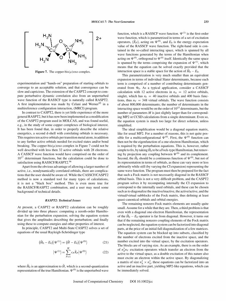
Figure 8. 1-cyanonaphtalene/pyridine exciplex.
holes and RAS3 electrons should be even, and RAS2 orbitals andelectrons are used for qualitatively correct description of any mul-ticonfigurational character and/or configuration differences amongstates. This also makes sense if the RAS1 and RAS3 spaces areregarded to compute correlation of a mixed dynamic/nondynamiccharacter, or dynamic correlation that is strongly coupled to the non-dynamic correlation. So far, the approach has usually been to allowtwo holes in RAS1 and two electrons in RAS3, which is usuallydenoted as “SD”, and if affordable, four of each (SDTQ). However,for good reasons, the orbital optimization in the RASSCF becomesproblematic in the latter case. We would recommend that SDTQcalculations are performed using RASSCF orbitals from the SDcalculation, without further reoptimization. Also, what about calcu-lations with, e.g., up to four holes, but allowing only two electrons?Also, is the “even-number” restriction always the best? The field isopen for experiments.
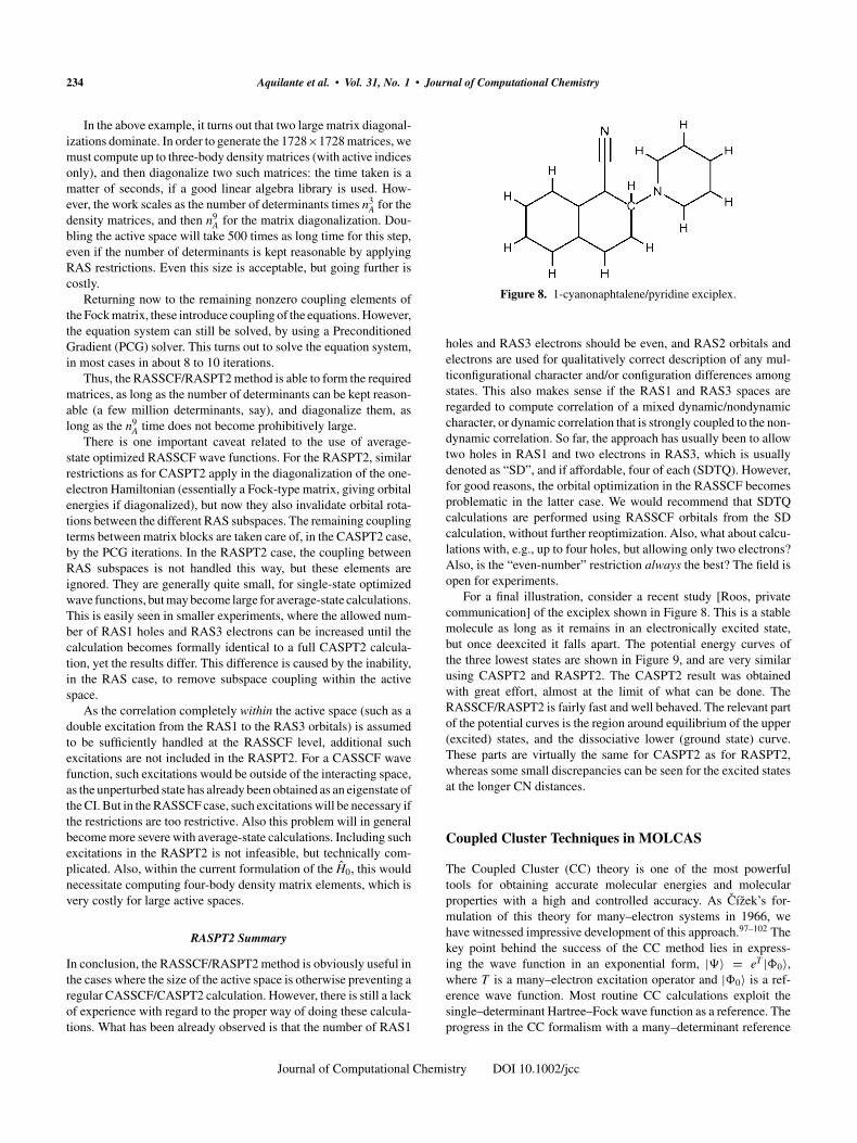
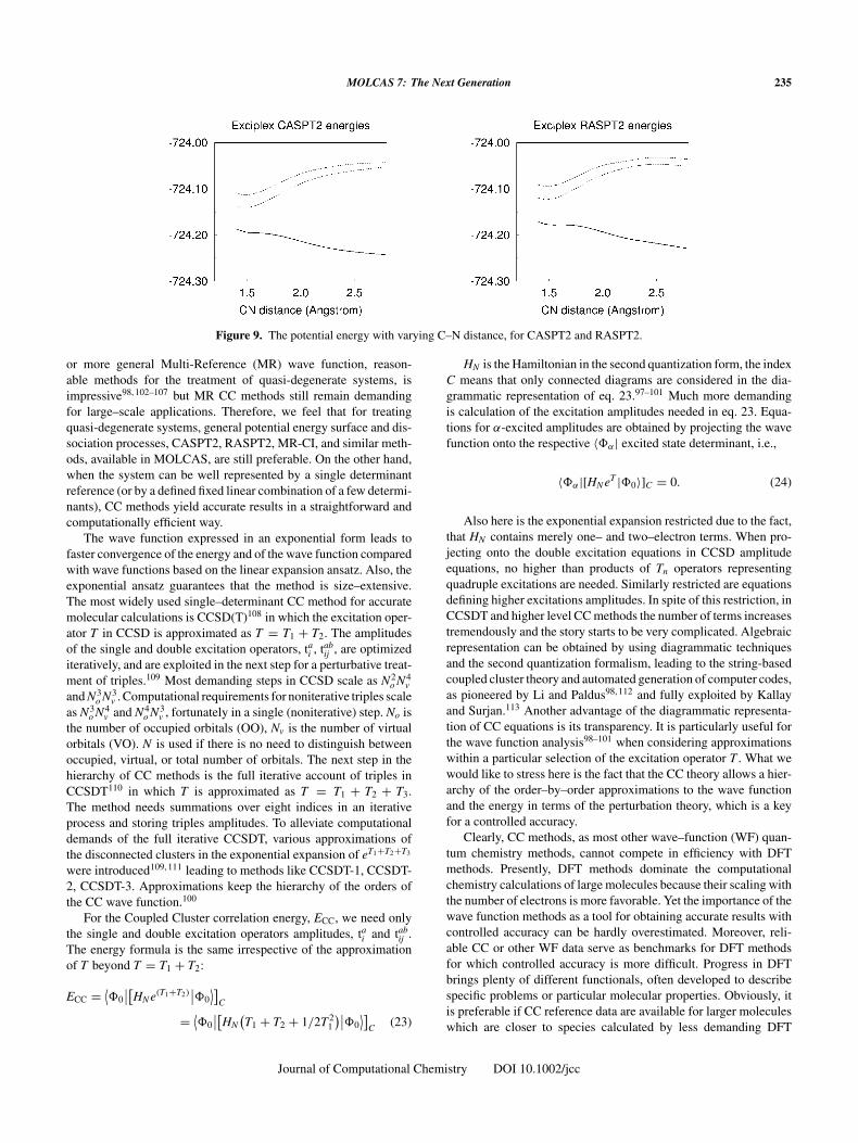
For a final illustration, consider a recent study [Roos, privatecommunication] of the exciplex shown in Figure 8. This is a stablemolecule as long as it remains in an electronically excited state,but once deexcited it falls apart. The potential energy curves ofthe three lowest states are shown in Figure 9, and are very similarusing CASPT2 and RASPT2. The CASPT2 result was obtainedwith great effort, almost at the limit of what can be done. TheRASSCF/RASPT2 is fairly fast and well behaved. The relevant partof the potential curves is the region around equilibrium of the upper(excited) states, and the dissociative lower (ground state) curve.These parts are virtually the same for CASPT2 as for RASPT2,whereas some small discrepancies can be seen for the excited statesat the longer CN distances.
Coupled Cluster Techniques in MOLCAS
The Coupled Cluster (CC) theory is one of the most powerfultools for obtaining accurate molecular energies and molecularproperties with a high and controlled accuracy. As Cížek’s for-mulation of this theory for many–electron systems in 1966, wehave witnessed impressive development of this approach.97–102 Thekey point behind the success of the CC method lies in express-ing the wave function in an exponential form, |�〉 = eT |�0〉,where T is a many–electron excitation operator and |�0〉 is a ref-erence wave function. Most routine CC calculations exploit thesingle–determinant Hartree–Fock wave function as a reference. Theprogress in the CC formalism with a many–determinant reference
Journal of Computational Chemistry DOI 10.1002/jcc
MOLCAS 7: The Next Generation 235
Figure 9. The potential energy with varying C–N distance, for CASPT2 and RASPT2.
or more general Multi-Reference (MR) wave function, reason-able methods for the treatment of quasi-degenerate systems, isimpressive98, 102–107 but MR CC methods still remain demandingfor large–scale applications. Therefore, we feel that for treatingquasi-degenerate systems, general potential energy surface and dis-sociation processes, CASPT2, RASPT2, MR-CI, and similar meth-ods, available in MOLCAS, are still preferable. On the other hand,when the system can be well represented by a single determinantreference (or by a defined fixed linear combination of a few determi-nants), CC methods yield accurate results in a straightforward andcomputationally efficient way.
The wave function expressed in an exponential form leads tofaster convergence of the energy and of the wave function comparedwith wave functions based on the linear expansion ansatz. Also, theexponential ansatz guarantees that the method is size–extensive.The most widely used single–determinant CC method for accuratemolecular calculations is CCSD(T)108 in which the excitation oper-ator T in CCSD is approximated as T = T1 + T2. The amplitudesof the single and double excitation operators, tai , tab
ij , are optimizediteratively, and are exploited in the next step for a perturbative treat-ment of triples.109 Most demanding steps in CCSD scale as N2
o N4v
and N3o N3
v . Computational requirements for noniterative triples scaleas N3
o N4v and N4
o N3v , fortunately in a single (noniterative) step. No is
the number of occupied orbitals (OO), Nv is the number of virtualorbitals (VO). N is used if there is no need to distinguish betweenoccupied, virtual, or total number of orbitals. The next step in thehierarchy of CC methods is the full iterative account of triples inCCSDT110 in which T is approximated as T = T1 + T2 + T3.The method needs summations over eight indices in an iterativeprocess and storing triples amplitudes. To alleviate computationaldemands of the full iterative CCSDT, various approximations ofthe disconnected clusters in the exponential expansion of eT1+T2+T3
were introduced109, 111 leading to methods like CCSDT-1, CCSDT-2, CCSDT-3. Approximations keep the hierarchy of the orders ofthe CC wave function.100
For the Coupled Cluster correlation energy, ECC, we need onlythe single and double excitation operators amplitudes, tai and tab
ij .The energy formula is the same irrespective of the approximationof T beyond T = T1 + T2:
ECC = ⟨�0
∣∣[HN e(T1+T2)∣∣�0
⟩]C
= ⟨�0
∣∣[HN(T1 + T2 + 1/2T2
1
)∣∣�0⟩]
C (23)
HN is the Hamiltonian in the second quantization form, the indexC means that only connected diagrams are considered in the dia-grammatic representation of eq. 23.97–101 Much more demandingis calculation of the excitation amplitudes needed in eq. 23. Equa-tions for α-excited amplitudes are obtained by projecting the wavefunction onto the respective 〈�α| excited state determinant, i.e.,
〈�α|[HN eT |�0〉]C = 0. (24)
Also here is the exponential expansion restricted due to the fact,that HN contains merely one– and two–electron terms. When pro-jecting onto the double excitation equations in CCSD amplitudeequations, no higher than products of Tn operators representingquadruple excitations are needed. Similarly restricted are equationsdefining higher excitations amplitudes. In spite of this restriction, inCCSDT and higher level CC methods the number of terms increasestremendously and the story starts to be very complicated. Algebraicrepresentation can be obtained by using diagrammatic techniquesand the second quantization formalism, leading to the string-basedcoupled cluster theory and automated generation of computer codes,as pioneered by Li and Paldus98, 112 and fully exploited by Kallayand Surjan.113 Another advantage of the diagrammatic representa-tion of CC equations is its transparency. It is particularly useful forthe wave function analysis98–101 when considering approximationswithin a particular selection of the excitation operator T . What wewould like to stress here is the fact that the CC theory allows a hier-archy of the order–by–order approximations to the wave functionand the energy in terms of the perturbation theory, which is a keyfor a controlled accuracy.
Clearly, CC methods, as most other wave–function (WF) quan-tum chemistry methods, cannot compete in efficiency with DFTmethods. Presently, DFT methods dominate the computationalchemistry calculations of large molecules because their scaling withthe number of electrons is more favorable. Yet the importance of thewave function methods as a tool for obtaining accurate results withcontrolled accuracy can be hardly overestimated. Moreover, reli-able CC or other WF data serve as benchmarks for DFT methodsfor which controlled accuracy is more difficult. Progress in DFTbrings plenty of different functionals, often developed to describespecific problems or particular molecular properties. Obviously, itis preferable if CC reference data are available for larger moleculeswhich are closer to species calculated by less demanding DFT
Journal of Computational Chemistry DOI 10.1002/jcc
236 Aquilante et al. • Vol. 31, No. 1 • Journal of Computational Chemistry
calculations. To serve this purpose better, we need CC methods,particularly CCSD(T) with enhanced efficiency within MOLCAS.
Open–Shell Calculations
The open–shell CC program in MOLCAS was primarily devel-oped for efficient treatment of the high–spin systems which canbe well represented by a single–determinant Restricted Open–shell Hartree–Fock (ROHF) reference. The two determinant CCSDmethod is introduced in MOLCAS for treating excited singlets.114
As the contribution from triples is still missing, this part of the codeis not widely used so far. Starting point of our high–spin implementa-tion is the spin–orbital formulation of Stanton et al.115 Fully relyingon the spin-orbital formulation means, first, lower efficiency, as onehas to manage spin–orbitals instead of orbitals and, second, result-ing CCSD(T) energy is affected by the spin contamination even ifwe use the ROHF reference orbitals. We also note that the ROHFreference function is not uniquely defined. There is certain degreeof freedom in construction of the one–electron part of the Hamilto-nian, fR, which does not change the SCF energy, but affects orbitalenergies. The iterative CCSD procedure itself is fully invariant tosplitting of the Fock operator f = fR + u. However, perturbativeenergy terms are not, due to using orbital energies in denominators.Therefore, also noniterative T3 contribution, evaluated in a pertur-bational manner, slightly depends on the selection of the referencefunction and the denominator. For details, see e.g. ref. 116,117 andcareful discussion in ref. 118
The ROHF reference function is an eigenfunction of the spinoperators S2 and Sz, but the CC wave function exp(T)|�0〉 is not, ifthe CC expansion (or the T operator) is not complete. The magni-tude of the spin contamination diminishes with higher levels of theexcitation operators. Amplitudes of the single and double excitationoperators in CCSD, tai , tab
ij , must be spin adapted. Spin adapta-tion (SA) also reduces the number of independent parameters (i.e.,excitation amplitudes), by about a factor of three for CCSD, andenhances the efficiency, if fully exploited. In our implementationin MOLCAS we have profited from the work by Takahashi andPaldus.119 We employ an approximate SA, particularly the sim-plest form in which only T2 amplitudes, labelled by inactive andsecondary orbitals are adopted (active orbitals would be singly occu-pied MOs, using the terminology of CASSCF). This approximatemethod116, 117 preserves most of the advantages of the spin adapta-tion, is sufficiently accurate (compare with exact results by Gaussand Szalay120) and the formulation is the same for any multiplet.Effects of the spin–adaptation in molecular properties are usuallysmall. More difficult cases, like CCSD(T) calculation of the electronaffinity of the CN or O2 molecules require SA for accurate results.
Efficiency of CC Calculations
The present version of the MOLCAS package contains two imple-mentations of CCSD(T) method: An older code, described alreadyin previous MOLCAS paper26 and a new one, based on Choleskydecomposition of the two–electron integrals. The old implementa-tion of the CCSD method was based on the formulation115 whichexploits spin–orbital formalism aimed toward minimizing the over-all number of floating-point operations. The code exploits orbitalspatial symmetry and is compatible with both RHF and ROHF ref-erence functions. It is optimal though for open–shell molecules only,
whereas a different algorithm could exploit simplifications arisingin the closed–shell case. Program handles arrays up to the sizeof N2
o N2v in an unsegmented form, which ensures relatively small
computational overhead. This feature, combined with the efficientmatrix–matrix oriented formulation and BLAS (level 3) routinesguarantees high performance of the arithmetical part. Being com-pletely MO based, this algorithm required storing all MO integrals(proportional to N4) on disk. Also memory consumption cannot bearbitrarily reduced, as the N2
o N2v arrays are treated as unsegmented.
Moreover, the way the code was parallelized, allowed efficient (closeto linear) scaling only up to 8–16 nodes. All these factors causeserious limitations of its applicability. Typically, calculations do notexceed 500 virtual orbitals and the performance strongly dependson the computer hardware, the number of the correlated electrons,computational symmetry, and the distribution of molecular orbitalswithin irreducible representations of the symmetry point group. Tofurther enhance the applicability of the CCSD(T) method, a com-pletely new code was implemented. It is based on two novel ideas,mainly the Cholesky decomposition of two electron integrals andthe segmentation (or blocking) of the virtual orbital space (VOS).
To reduce or, eventually, completely eliminate the memory lim-itations and to utilize efficient parallelization we decided to splitthe VOS into N ′ segments, each having Nv ′ = Nv/N ′ orbitals.Memory requirements are dramatically reduced, since for all inter-mediates having at least one virtual index, we can work with theirfragments with reduced dimension of Nv ′ instead of Nv. This affectsmostly the time consuming N6 matrix multiplications, which aresplit into N ′2 “independent” subjobs of almost the same size. Asa byproduct, splitting offers a possibility for the efficient (almostlinear) parallelization, employing up to N ′2 computational nodes.However, parallelization and segmentation of the VOS brings insome additional overhead, due to repeated (mostly I/O) opera-tions connected with the segmentation in the matrix multiplicationprocess. The only internode transfer required in this new CCSDalgorithm is the transfer of T1 and T2 amplitudes in each itera-tion. The wall–clock time needed for this transfer increases with thenumber of parallel nodes, though less than linearly. Thus, due tothis connection of segmentation and the number of parallel tasks,proper N ′ needs to be selected (presently as a user-defined param-eter) to meet the memory requirements and to ensure efficientparallelization.
Cholesky decomposition of integrals cannot, in general, reducethe scaling of the most time consuming steps in the CC methods.However, storing only the (MO-transformed) Cholesky vectors alle-viates one important bottleneck of the CCSD(T) approach, e.g., thestorage of the 2-electron integrals, and offers additional flexibilitywhenever the reconstruction of these integrals is needed. This con-cerns mainly the (VV |VV) (scaling as N4
v ) and (OV |VV) (scalingas N3
v No) integral types, where V stands for arbitrary index of vir-tual orbital and O for the occupied one. A different treatment toavoid the disk bottleneck, widely used in other CCSD codes, is socalled “integral direct” algorithm,121 which essentially calculateson–the–fly all the required AO integrals. These approaches have,however, a disadvantage compared with our MO Cholesky vectorsbased CCSD code that, the CCSD equations are solved in the AObasis and cannot profit so much from the truncation of the virtualorbital space either via OVOS method of Frozen Natural Orbitals,see further.
Journal of Computational Chemistry DOI 10.1002/jcc
MOLCAS 7: The Next Generation 237
In our new CCSD code, two basic algorithms for treating themost demanding (VV |VV) integrals are implemented and are avail-able on user’s choice. Both employ segmentation governed by thesize of the (V ′V ′|V ′V ′) block. In the first approach we do not storeany integral files larger than N2
o N2v on the disk and desired integral
blocks are recalculated from Cholesky vectors, eq. 12, on the fly.This yields enormous savings of the disk space, but overall arithmeti-cal demands increase. On the other hand, this “purely CD based”approach, with suppressed I/O and extended arithmetics can betterexploit modern multi-core architecture of the nodes, than the “inte-gral based” one. In the alternative “integral based” approach weprecalculate most of the MO integrals (including (VV |VV)) fromthe Cholesky vectors, eq. 12, before the CCSD iterative procedureand store them on the disk. Taking advantage of how the Choleskydecomposition of the two-electron integrals is implemented in theparallel version of MOLCAS, namely that Cholesky vectors aregenerated on each computational node in blocks according to thesegmented auxiliary index, precalculation of above mentioned inte-grals can be efficiently parallelized as well. CCSD equations arethen solved essentially in the “traditional,” MO–based way. This“integral based” algorithm is preferable either if there is an abun-dance of the disk space, or in the massively parallel runs, wheredue to the way the algorithm is implemented, only a small por-tion of the MO integrals needs to be stored on each parallel node.For smaller calculations it is typically faster than “purely CD based”approach, however, for truly large scale calculations with N2
o compa-rable to M (dimension of the Cholesky auxiliary index), “purely CDbased” approach becomes preferable. MO transformed Choleskyvectors are also employed in the elimination of tedious manipula-tions with the (OV |VV) integrals. Several terms, containing this typeof integrals, can be treated together with terms containing (VV |VV)
integrals in a single step. The rest of these terms can be reformulatedusing LJ
pq vectors. Even if the scaling is not reduced, any manipula-tions with (OV |VV) integrals can be fully avoided in this way. Forexample, the contribution
tabij ←
∑c
(ai|bc)tcj (25)
can be performed as
AJbj =
∑c
LJbctc
j (26)
tabij ←
∑J
LJaiA
Jbj (27)
Procedure 26–27 needs MNoN2v + MN2
v N2o operations, i.e., about
M/Nv times more than procedure 25, however manipulations with(OV |VV) integrals is completely eliminated. The excess of thearithmetics is not large, because all terms of this kind scale atmost as N5.
Generally, efficiency of parallelization of the CCSD algorithmdepends on the size of the system. It is efficient, if the “wall–clockportion” of calculation of the N6 steps on each node is larger than theoverhead resulting mostly from the internode data transfer, whichscales basically as N4. The larger the system is, the more efficient
is the parallelization, as the calculation spends less time with thedata transfer. For a systems with about 1000 basis functions, ournew CCSD code is efficient even for hundreds of parallel nodes.Performance of the new code will be described in details elsewhere(Neogrády et al., to be published).
For systems with large number of correlated electrons, the non-iterative (T) part becomes by far the most time consuming step.For evaluation of the (T) contribution, our new CCSD code wasextended with the essential routines adapted to MOLCAS from thecode programmed by Noga and Valiron.122 Also here, segmentationof the VOS is used. Algorithm for (T) can be very well parallelized,because it can be split into large number of independent subjobs,with almost no communication among the nodes. Number of subjobsdepends on the number of occupied orbitals, not on N ′. Much moreefficient parallelization can be achieved, compared to the CCSDstep, which can to some extent compensate its order–of–magnitudehigher scaling (N7), almost prohibitive for large calculations.
The new suite of CC codes is presently fully implemented onlyfor closed shell systems in the spin integrated form123 with theminimized number of arithmetic operations. A code, with a similarcapabilities, for open–shell systems is currently under development.Several groups tried to resolve limitations of conventional CCSD(T)approaches. Gordon,124 Pulay125, 126 and Bartlett127 and theircoworkers have announced new implementations of the CCSD(T)codes optimal for massive parallelization and memory requirements.Comparison of the efficiency of various implementations is notavailable to us. Concerning new approaches for perturbative triples,several appealing attempts were published during the past fewyears. A common feature of these approaches is the decomposition(either in the Laplace or Cholesky fashion) of the energy denomi-nators. Although the Cholesky decomposition–based approach byKoch et al.128 seems to be more efficient for systems with highratio of occupied to virtual orbitals, Laplace decomposition–basedapproaches suggested by Scuseria and Head-Gordon groups utilizeprescreening of certain intermediates transformed to either Natu-ral Orbitals123, 129 or into localized, atom-labelled projected orbitalbasis130). Both approaches have capability of reducing the scaling ofperturbative triples from N7 to N5, but more robust implementationsare desirable for extensive applications.
Optimizing and Reducing the Space of Virtual Orbitals (OVOS)
Cholesky decomposition and high level of parallelism is a prerequi-site for using CCSD(T) within MOLCAS for larger applications thanit was possible before. Nevertheless, we still need to look at alterna-tive ways leading to reduced computational demands. Unfavorablescaling with the number of virtual orbitals N4
v in most difficult stepsin CCSD and triples makes calculations with large Nv quickly pro-hibitive. Another bottleneck is the number of occupied orbitals whenwe need to correlate large number of electrons. Large Nv frequentlyoccurs in calculations with extended (diffuse) basis sets for accu-rate calculations of, say, response properties, excited (particularlyRydberg) states, electron affinities, dispersion interactions, etc. Dowe really need an extended full space of virtual orbitals selected withno condition other than being orthogonal to (canonical) HF occupiedorbitals? The simplest way, deleting just a few virtuals with highestorbital energies is of little help. Truncation of VOS to a significantfraction, say one half, may already reduce the N4
v steps by a factor
Journal of Computational Chemistry DOI 10.1002/jcc
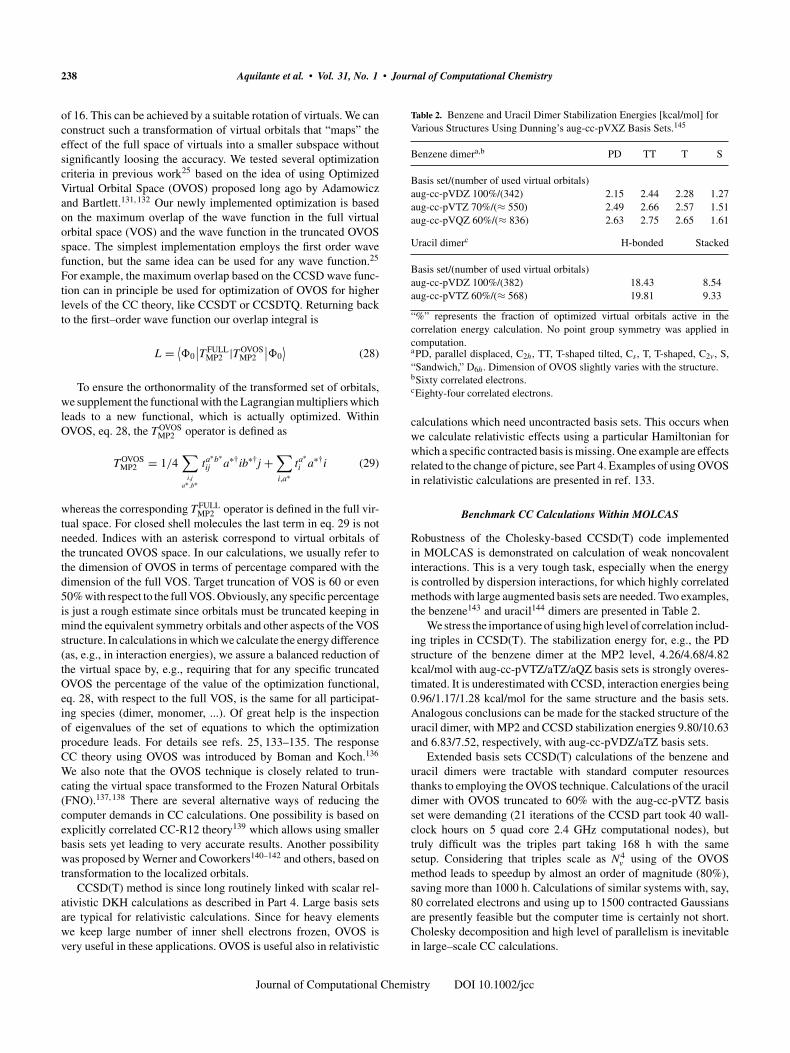
238 Aquilante et al. • Vol. 31, No. 1 • Journal of Computational Chemistry
of 16. This can be achieved by a suitable rotation of virtuals. We canconstruct such a transformation of virtual orbitals that “maps” theeffect of the full space of virtuals into a smaller subspace withoutsignificantly loosing the accuracy. We tested several optimizationcriteria in previous work25 based on the idea of using OptimizedVirtual Orbital Space (OVOS) proposed long ago by Adamowiczand Bartlett.131, 132 Our newly implemented optimization is basedon the maximum overlap of the wave function in the full virtualorbital space (VOS) and the wave function in the truncated OVOSspace. The simplest implementation employs the first order wavefunction, but the same idea can be used for any wave function.25
For example, the maximum overlap based on the CCSD wave func-tion can in principle be used for optimization of OVOS for higherlevels of the CC theory, like CCSDT or CCSDTQ. Returning backto the first–order wave function our overlap integral is
L = ⟨�0
∣∣TFULLMP2 |TOVOS
MP2
∣∣�0⟩
(28)
To ensure the orthonormality of the transformed set of orbitals,we supplement the functional with the Lagrangian multipliers whichleads to a new functional, which is actually optimized. WithinOVOS, eq. 28, the TOVOS
MP2 operator is defined as
TOVOSMP2 = 1/4
∑i,j
a∗ ,b∗
ta∗b∗ij a∗†ib∗†j +
∑i,a∗
ta∗i a∗†i (29)
whereas the corresponding TFULLMP2 operator is defined in the full vir-
tual space. For closed shell molecules the last term in eq. 29 is notneeded. Indices with an asterisk correspond to virtual orbitals ofthe truncated OVOS space. In our calculations, we usually refer tothe dimension of OVOS in terms of percentage compared with thedimension of the full VOS. Target truncation of VOS is 60 or even50% with respect to the full VOS. Obviously, any specific percentageis just a rough estimate since orbitals must be truncated keeping inmind the equivalent symmetry orbitals and other aspects of the VOSstructure. In calculations in which we calculate the energy difference(as, e.g., in interaction energies), we assure a balanced reduction ofthe virtual space by, e.g., requiring that for any specific truncatedOVOS the percentage of the value of the optimization functional,eq. 28, with respect to the full VOS, is the same for all participat-ing species (dimer, monomer, ...). Of great help is the inspectionof eigenvalues of the set of equations to which the optimizationprocedure leads. For details see refs. 25, 133–135. The responseCC theory using OVOS was introduced by Boman and Koch.136
We also note that the OVOS technique is closely related to trun-cating the virtual space transformed to the Frozen Natural Orbitals(FNO).137, 138 There are several alternative ways of reducing thecomputer demands in CC calculations. One possibility is based onexplicitly correlated CC-R12 theory139 which allows using smallerbasis sets yet leading to very accurate results. Another possibilitywas proposed by Werner and Coworkers140–142 and others, based ontransformation to the localized orbitals.
CCSD(T) method is since long routinely linked with scalar rel-ativistic DKH calculations as described in Part 4. Large basis setsare typical for relativistic calculations. Since for heavy elementswe keep large number of inner shell electrons frozen, OVOS isvery useful in these applications. OVOS is useful also in relativistic
Table 2. Benzene and Uracil Dimer Stabilization Energies [kcal/mol] forVarious Structures Using Dunning’s aug-cc-pVXZ Basis Sets.145
Benzene dimera,b PD TT T S
Basis set/(number of used virtual orbitals)aug-cc-pVDZ 100%/(342) 2.15 2.44 2.28 1.27aug-cc-pVTZ 70%/(≈ 550) 2.49 2.66 2.57 1.51aug-cc-pVQZ 60%/(≈ 836) 2.63 2.75 2.65 1.61
Uracil dimerc H-bonded Stacked
Basis set/(number of used virtual orbitals)aug-cc-pVDZ 100%/(382) 18.43 8.54aug-cc-pVTZ 60%/(≈ 568) 19.81 9.33
“%” represents the fraction of optimized virtual orbitals active in thecorrelation energy calculation. No point group symmetry was applied incomputation.aPD, parallel displaced, C2h, TT, T-shaped tilted, Cs, T, T-shaped, C2v, S,“Sandwich,” D6h. Dimension of OVOS slightly varies with the structure.bSixty correlated electrons.cEighty-four correlated electrons.
calculations which need uncontracted basis sets. This occurs whenwe calculate relativistic effects using a particular Hamiltonian forwhich a specific contracted basis is missing. One example are effectsrelated to the change of picture, see Part 4. Examples of using OVOSin relativistic calculations are presented in ref. 133.
Benchmark CC Calculations Within MOLCAS
Robustness of the Cholesky-based CCSD(T) code implementedin MOLCAS is demonstrated on calculation of weak noncovalentinteractions. This is a very tough task, especially when the energyis controlled by dispersion interactions, for which highly correlatedmethods with large augmented basis sets are needed. Two examples,the benzene143 and uracil144 dimers are presented in Table 2.
We stress the importance of using high level of correlation includ-ing triples in CCSD(T). The stabilization energy for, e.g., the PDstructure of the benzene dimer at the MP2 level, 4.26/4.68/4.82kcal/mol with aug-cc-pVTZ/aTZ/aQZ basis sets is strongly overes-timated. It is underestimated with CCSD, interaction energies being0.96/1.17/1.28 kcal/mol for the same structure and the basis sets.Analogous conclusions can be made for the stacked structure of theuracil dimer, with MP2 and CCSD stabilization energies 9.80/10.63and 6.83/7.52, respectively, with aug-cc-pVDZ/aTZ basis sets.
Extended basis sets CCSD(T) calculations of the benzene anduracil dimers were tractable with standard computer resourcesthanks to employing the OVOS technique. Calculations of the uracildimer with OVOS truncated to 60% with the aug-cc-pVTZ basisset were demanding (21 iterations of the CCSD part took 40 wall-clock hours on 5 quad core 2.4 GHz computational nodes), buttruly difficult was the triples part taking 168 h with the samesetup. Considering that triples scale as N4
v using of the OVOSmethod leads to speedup by almost an order of magnitude (80%),saving more than 1000 h. Calculations of similar systems with, say,80 correlated electrons and using up to 1500 contracted Gaussiansare presently feasible but the computer time is certainly not short.Cholesky decomposition and high level of parallelism is inevitablein large–scale CC calculations.
Journal of Computational Chemistry DOI 10.1002/jcc
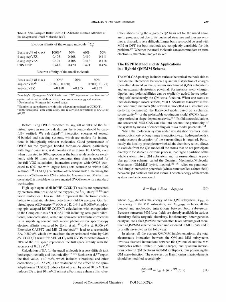
MOLCAS 7: The Next Generation 239
Table 3. Spin–Adapted ROHF CCSD(T) Adiabatic Electron Affinities ofthe Oxygen and Uracil Molecules [eV].
Electron affinity of the oxygen molecule, 3�−g
Basis set/(# of v. o.) 100%a 70% 60% 50%d-aug-ccpV5Z 0.403 0.408 0.410 0.411d-aug-ccpV6Z 0.407 0.408 0.412 0.418CBS limitc 0.415 0.420 0.421 0.424
Electron affinity of the uracil molecule
Basis set/(# of v. o.) 100%a 70% 60%aug-ccpVDZb −0.189(−0.160) −0.200(−0.177)
aug-ccpVTZ −0.150 −0.155 −0.157
Dunning’s (d)–aug-cc-pVXZ basis sets. “%” represents the fraction ofoptimized virtual orbitals active in the correlation energy calculation.aOne hundred % means full virtual space.bNumber in parentheses is with spin–adaptation omitted in CCSD(T).cWith vibrational, core correlation, and relativistic corrections is EA 0.449eV.146
Before using OVOS truncated to, say, 60 or 50% of the fullvirtual space in routine calculations the accuracy should be care-fully verified. We calculated134 interaction energies of severalH-bonded and stacking systems, which are models for interac-tions in biologically relevant molecules. Good performance ofOVOS for the hydrogen bonded formamide dimer, particularlywith larger basis sets, is demonstrated in Figure 10. OVOS, evenwhen truncated to 50%, reproduces the basis set dependence excel-lently with 10 times shorter computer time than is needed forthe full VOS calculation. Interaction energies with OVOS trun-cated to 60% are with largest basis sets accurate to within 0.02kcal/mol.134 CCSD(T) calculation of the formamide dimer using theaug-cc-pV5Z basis set (1242 contracted Gaussians and 36 electronscorrelated) is tractable with so truncated OVOS even with a standardworkstation.
High–spin open–shell ROHF–CCSD(T) results are representedby electron affinities (EA) of the oxygen (the 3�−
g state)135, 146 anduracil molecules. Data in Table 3 represent the electronic contri-bution to adiabatic electron detachment (AED) energies. Our fullvirtual space AED energy146 of O2 at 0 K, 0.449 ± 0.008 eV, employ-ing spin–adapted ROHF CCSD(T) calculations with extrapolationto the Complete Basis Set (CBS) limit including zero–point vibra-tional, core correlation, scalar and spin-orbit relativistic correctionsis in superb agreement with recent photoelectron spectroscopyelectron affinity measured by Ervin et al.,147 0.448 ± 0.006 eV.Extensive CASPT2 and MR CI methods148 lead to a reasonableEA, 0.389 eV, which deviates from the experimental value by 0.06eV. CCSD(T) result for AED of O2 with OVOS truncated down to50% of the full space reproduces the full space affinity with theaccuracy of 0.01 eV.135
Calculation of EA for the uracil molecule is a very difficult taskboth experimentally and theoretically.149–151 Bachorz et al.149 reportthe final value, +40 meV, which includes vibrational and othercorrections (+0.155 eV). Our treatment of the effect of the spin–adaptation in CCSD(T) reduces EA of uracil by about 30 meV. Thisreduces EA to just 10 meV. Basis set effects may enhance this value.
Calculations using the aug-cc-pVQZ basis set for the uracil anionare in progress, but due to its puckered structure and thus no sym-metry, this task is very difficult. Larger basis sets could be used withMP2 or DFT but both methods are completely unreliable for thisproblem.149 Whether the uracil molecule can accommodate an extraelectron is, therefore, not yet solved.
The ESPF Method and its Applicationsin a Hybrid QM/MM Scheme
The MOLCAS package includes various theoretical methods able toinclude the interactions between a quantum distribution of charges(hereafter denoted as the quantum mechanical (QM) subsystem)and an external electrostatic potential. For instance, point charges,dipoles, and polarizabilities can be explicitly added, hence polar-izing self-consistently the QM wave function. When one wants toinclude isotropic solvent effects, MOLCAS allows to use two differ-ent continuum methods (the solvent is modelled as a structurelessdielectric continuum): the Kirkwood model based on a sphericalsolute cavity152 or the polarizable continuum model (PCM) featur-ing a molecular shape-dependent cavity.153 If solid state calculationsare concerned, MOLCAS can take into account the periodicity ofthe system by means of embedding ab initio model potentials.154
When the molecular system under investigation features someanisotropic short- or long-range interactions (e.g., hydrogen bonds),a microscopic description of the surroundings is required. Fortu-nately, the locality principle on which all the chemistry relies, allowsto exclude from the QM model all the atoms that do not participatedirectly to the studied electronic process, leading to a partition of thewhole system into a QM subsystem and its surroundings. A pop-ular partition scheme, called the Quantum Mechanics/MolecularMechanics (QM/MM) hybrid method,155–157 relies on parameter-ized simple interaction potentials (whose sum is called a force-field)between QM particles and MM atoms. The total energy of the wholesystem can be decomposed:
E = EQM + EMM + EQM/MM (30)
where EQM denotes the energy of the QM subsystem, EMM isthe energy of the MM subsystem, and EQM/MM includes all thebonded and nonbonded interactions between both subsystems.Because numerous MM force-fields are already available in variouschemistry fields (organic chemistry, biochemistry, heterogeneouscatalysis, etc.), the QM/MM method often takes advantage of them.Such a QM/MM scheme has been implemented in MOLCAS and itis briefly presented in the following.
In almost all the current QM/MM implementations, the totalelectrostatic interaction between the QM and MM subsystemsinvolves classical interactions between the QM nuclei and the MMmultipoles (often limited to point charges) and quantum interac-tions between QM electrons and MM multipoles, thus polarizing theQM wave-function. The one-electron Hamiltonian matrix elementsshould be modified accordingly:
hQM/MMµν = hµν + 〈µ|VMM(r)|ν〉 (31)
Journal of Computational Chemistry DOI 10.1002/jcc
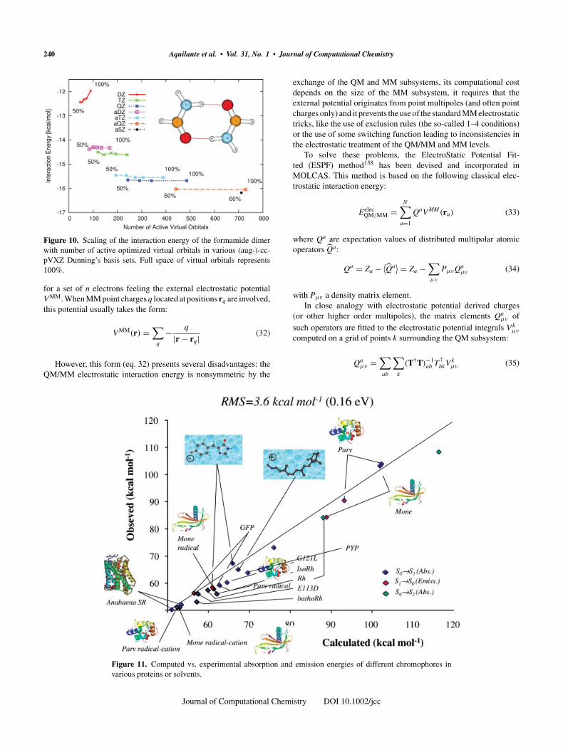
240 Aquilante et al. • Vol. 31, No. 1 • Journal of Computational Chemistry
Figure 10. Scaling of the interaction energy of the formamide dimerwith number of active optimized virtual orbitals in various (aug-)-cc-pVXZ Dunning’s basis sets. Full space of virtual orbitals represents100%.
for a set of n electrons feeling the external electrostatic potentialVMM. When MM point charges q located at positions rq are involved,this potential usually takes the form:
VMM(r) =∑
q
− q
|r − rq| (32)
However, this form (eq. 32) presents several disadvantages: theQM/MM electrostatic interaction energy is nonsymmetric by the
exchange of the QM and MM subsystems, its computational costdepends on the size of the MM subsystem, it requires that theexternal potential originates from point multipoles (and often pointcharges only) and it prevents the use of the standard MM electrostatictricks, like the use of exclusion rules (the so-called 1–4 conditions)or the use of some switching function leading to inconsistencies inthe electrostatic treatment of the QM/MM and MM levels.
To solve these problems, the ElectroStatic Potential Fit-ted (ESPF) method158 has been devised and incorporated inMOLCAS. This method is based on the following classical elec-trostatic interaction energy:
EelecQM/MM =
N∑a=1
QaVMM(ra) (33)
where Qa are expectation values of distributed multipolar atomicoperators Qa:
Qa = Za − ⟨Qa⟩ = Za −
∑µν
PµνQaµν (34)
with Pµν a density matrix element.In close analogy with electrostatic potential derived charges
(or other higher order multipoles), the matrix elements Qaµν of
such operators are fitted to the electrostatic potential integrals Vkµν
computed on a grid of points k surrounding the QM subsystem:
Qaµν =
∑ab
∑k
(T†T)−1ab T†
bkVkµν (35)
Figure 11. Computed vs. experimental absorption and emission energies of different chromophores invarious proteins or solvents.
Journal of Computational Chemistry DOI 10.1002/jcc
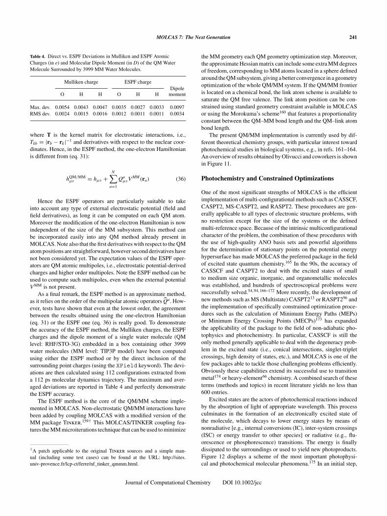
MOLCAS 7: The Next Generation 241
Table 4. Direct vs. ESPF Deviations in Mulliken and ESPF AtomicCharges (in e) and Molecular Dipole Moment (in D) of the QM WaterMolecule Surrounded by 3999 MM Water Molecules.
Mulliken charge ESPF chargeDipole
O H H O H H moment
Max. dev. 0.0054 0.0043 0.0047 0.0035 0.0027 0.0033 0.0097RMS dev. 0.0024 0.0015 0.0016 0.0012 0.0011 0.0011 0.0034
where T is the kernel matrix for electrostatic interactions, i.e.,Tkb = |rb − rk |−1 and derivatives with respect to the nuclear coor-dinates. Hence, in the ESPF method, the one-electron Hamiltonianis different from (eq. 31):
hQM/MMµν = hµν +
N∑a=1
QaµνVMM(ra) (36)
Hence the ESPF operators are particularly suitable to takeinto account any type of external electrostatic potential (field andfield derivatives), as long it can be computed on each QM atom.Moreover the modification of the one-electron Hamiltonian is nowindependent of the size of the MM subsystem. This method canbe incorporated easily into any QM method already present inMOLCAS. Note also that the first derivatives with respect to the QMatom positions are straightforward, however second derivatives havenot been considered yet. The expectation values of the ESPF oper-ators are QM atomic multipoles, i.e., electrostatic potential-derivedcharges and higher order multipoles. Note the ESPF method can beused to compute such multipoles, even when the external potentialVMM is not present.
As a final remark, the ESPF method is an approximate method,as it relies on the order of the multipolar atomic operators Qa. How-ever, tests have shown that even at the lowest order, the agreementbetween the results obtained using the one-electron Hamiltonian(eq. 31) or the ESPF one (eq. 36) is really good. To demonstratethe accuracy of the ESPF method, the Mulliken charges, the ESPFcharges and the dipole moment of a single water molecule (QMlevel: RHF/STO-3G) embedded in a box containing other 3999water molecules (MM level: TIP3P model) have been computedusing either the ESPF method or by the direct inclusion of thesurrounding point charges (using the XField keyword). The devi-ations are then calculated using 112 configurations extracted froma 112 ps molecular dynamics trajectory. The maximum and aver-aged deviations are reported in Table 4 and perfectly demonstratethe ESPF accuracy.
The ESPF method is the core of the QM/MM scheme imple-mented in MOLCAS. Non-electrostatic QM/MM interactions havebeen added by coupling MOLCAS with a modified version of theMM package Tinker.159† This MOLCAS/TINKER coupling fea-tures the MM microiterations technique that can be used to minimize
†A patch applicable to the original Tinker sources and a simple man-ual (including some test cases) can be found at the URL: http://sites.univ-provence.fr/lcp-ct/ferre/nf_tinker_qmmm.html.
the MM geometry each QM geometry optimization step. Moreover,the approximate Hessian matrix can include some extra MM degreesof freedom, corresponding to MM atoms located in a sphere definedaround the QM subsystem, giving a better convergence in a geometryoptimization of the whole QM/MM system. If the QM/MM frontieris located on a chemical bond, the link atom scheme is available tosaturate the QM free valence. The link atom position can be con-strained using standard geometry constraint available in MOLCASor using the Morokuma’s scheme160 that features a proportionalityconstant between the QM–MM bond length and the QM–link atombond length.
The present QM/MM implementation is currently used by dif-ferent theoretical chemistry groups, with particular interest towardphotochemical studies in biological systems, e.g., in refs. 161–164.An overview of results obtained by Olivucci and coworkers is shownin Figure 11.
Photochemistry and Constrained Optimizations
One of the most significant strengths of MOLCAS is the efficientimplementation of multi-configurational methods such as CASSCF,CASPT2, MS-CASPT2, and RASPT2. These procedures are gen-erally applicable to all types of electronic structure problems, withno restriction except for the size of the systems or the definedmulti-reference space. Because of the intrinsic multiconfigurationalcharacter of the problem, the combination of these procedures withthe use of high-quality ANO basis sets and powerful algorithmsfor the determination of stationary points on the potential energyhypersurface has made MOLCAS the preferred package in the fieldof excited state quantum chemistry.165 In the 90s, the accuracy ofCASSCF and CASPT2 to deal with the excited states of smallto medium size organic, inorganic, and organometallic moleculeswas established, and hundreds of spectroscopical problems weresuccessfully solved.54, 94, 166–172 More recently, the development ofnew methods such as MS (Multistate) CASPT213 or RASPT296 andthe implementation of specifically constrained optimization proce-dures such as the calculation of Minimum Energy Paths (MEPs)or Minimum Energy Crossing Points (MECPs)173 has expandedthe applicability of the package to the field of non-adiabatic pho-tophysics and photochemistry. In particular, CASSCF is still theonly method generally applicable to deal with the degeneracy prob-lem in the excited state (i.e., conical intersections, singlet-tripletcrossings, high density of states, etc.), and MOLCAS is one of thefew packages able to tackle those challenging problems efficiently.Obviously these capabilities extend its successful use to transitionmetal174 or heavy-element66 chemistry. A combined search of theseterms (methods and topics) in recent literature yields no less than600 entries.
Excited states are the actors of photochemical reactions inducedby the absorption of light of appropriate wavelength. This processculminates in the formation of an electronically excited state ofthe molecule, which decays to lower energy states by means ofnonradiative [e.g., internal conversions (IC), inter-system crossings(ISC) or energy transfer to other species] or radiative (e.g., flu-orescence or phosphorescence) transitions. The energy is finallydissipated to the surroundings or used to yield new photoproducts.Figure 12 displays a scheme of the most important photophysi-cal and photochemical molecular phenomena.175 In an initial step,
Journal of Computational Chemistry DOI 10.1002/jcc
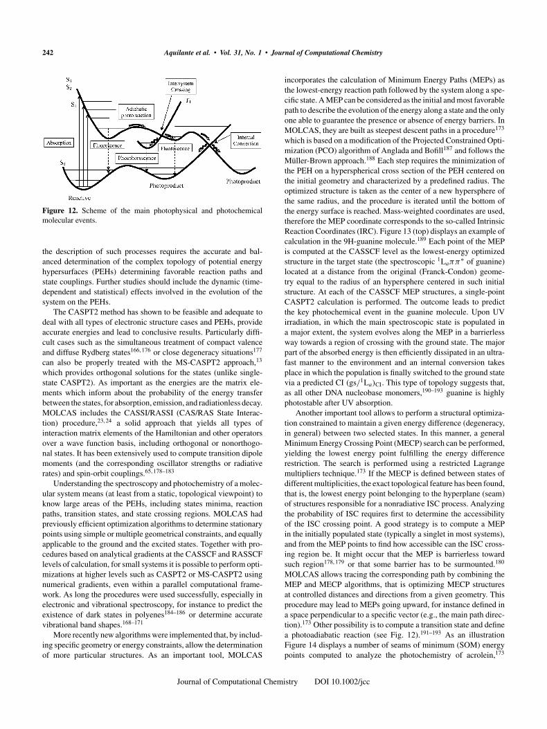
242 Aquilante et al. • Vol. 31, No. 1 • Journal of Computational Chemistry
Figure 12. Scheme of the main photophysical and photochemicalmolecular events.
the description of such processes requires the accurate and bal-anced determination of the complex topology of potential energyhypersurfaces (PEHs) determining favorable reaction paths andstate couplings. Further studies should include the dynamic (time-dependent and statistical) effects involved in the evolution of thesystem on the PEHs.
The CASPT2 method has shown to be feasible and adequate todeal with all types of electronic structure cases and PEHs, provideaccurate energies and lead to conclusive results. Particularly diffi-cult cases such as the simultaneous treatment of compact valenceand diffuse Rydberg states166, 176 or close degeneracy situations177
can also be properly treated with the MS-CASPT2 approach,13
which provides orthogonal solutions for the states (unlike single-state CASPT2). As important as the energies are the matrix ele-ments which inform about the probability of the energy transferbetween the states, for absorption, emission, and radiationless decay.MOLCAS includes the CASSI/RASSI (CAS/RAS State Interac-tion) procedure,23, 24 a solid approach that yields all types ofinteraction matrix elements of the Hamiltonian and other operatorsover a wave function basis, including orthogonal or nonorthogo-nal states. It has been extensively used to compute transition dipolemoments (and the corresponding oscillator strengths or radiativerates) and spin-orbit couplings.65, 178–183
Understanding the spectroscopy and photochemistry of a molec-ular system means (at least from a static, topological viewpoint) toknow large areas of the PEHs, including states minima, reactionpaths, transition states, and state crossing regions. MOLCAS hadpreviously efficient optimization algorithms to determine stationarypoints using simple or multiple geometrical constraints, and equallyapplicable to the ground and the excited states. Together with pro-cedures based on analytical gradients at the CASSCF and RASSCFlevels of calculation, for small systems it is possible to perform opti-mizations at higher levels such as CASPT2 or MS-CASPT2 usingnumerical gradients, even within a parallel computational frame-work. As long the procedures were used successfully, especially inelectronic and vibrational spectroscopy, for instance to predict theexistence of dark states in polyenes184–186 or determine accuratevibrational band shapes.168–171
More recently new algorithms were implemented that, by includ-ing specific geometry or energy constraints, allow the determinationof more particular structures. As an important tool, MOLCAS
incorporates the calculation of Minimum Energy Paths (MEPs) asthe lowest-energy reaction path followed by the system along a spe-cific state. A MEP can be considered as the initial and most favorablepath to describe the evolution of the energy along a state and the onlyone able to guarantee the presence or absence of energy barriers. InMOLCAS, they are built as steepest descent paths in a procedure173
which is based on a modification of the Projected Constrained Opti-mization (PCO) algorithm of Anglada and Bofill187 and follows theMüller-Brown approach.188 Each step requires the minimization ofthe PEH on a hyperspherical cross section of the PEH centered onthe initial geometry and characterized by a predefined radius. Theoptimized structure is taken as the center of a new hypersphere ofthe same radius, and the procedure is iterated until the bottom ofthe energy surface is reached. Mass-weighted coordinates are used,therefore the MEP coordinate corresponds to the so-called IntrinsicReaction Coordinates (IRC). Figure 13 (top) displays an example ofcalculation in the 9H-guanine molecule.189 Each point of the MEPis computed at the CASSCF level as the lowest-energy optimizedstructure in the target state (the spectroscopic 1Laππ∗ of guanine)located at a distance from the original (Franck-Condon) geome-try equal to the radius of an hypersphere centered in such initialstructure. At each of the CASSCF MEP structures, a single-pointCASPT2 calculation is performed. The outcome leads to predictthe key photochemical event in the guanine molecule. Upon UVirradiation, in which the main spectroscopic state is populated ina major extent, the system evolves along the MEP in a barrierlessway towards a region of crossing with the ground state. The majorpart of the absorbed energy is then efficiently dissipated in an ultra-fast manner to the environment and an internal conversion takesplace in which the population is finally switched to the ground statevia a predicted CI (gs/1La)CI. This type of topology suggests that,as all other DNA nucleobase monomers,190–193 guanine is highlyphotostable after UV absorption.
Another important tool allows to perform a structural optimiza-tion constrained to maintain a given energy difference (degeneracy,in general) between two selected states. In this manner, a generalMinimum Energy Crossing Point (MECP) search can be performed,yielding the lowest energy point fulfilling the energy differencerestriction. The search is performed using a restricted Lagrangemultipliers technique.173 If the MECP is defined between states ofdifferent multiplicities, the exact topological feature has been found,that is, the lowest energy point belonging to the hyperplane (seam)of structures responsible for a nonradiative ISC process. Analyzingthe probability of ISC requires first to determine the accessibilityof the ISC crossing point. A good strategy is to compute a MEPin the initially populated state (typically a singlet in most systems),and from the MEP points to find how accessible can the ISC cross-ing region be. It might occur that the MEP is barrierless towardsuch region178, 179 or that some barrier has to be surmounted.180
MOLCAS allows tracing the corresponding path by combining theMEP and MECP algorithms, that is optimizing MECP structuresat controlled distances and directions from a given geometry. Thisprocedure may lead to MEPs going upward, for instance defined ina space perpendicular to a specific vector (e.g., the main path direc-tion).173 Other possibility is to compute a transition state and definea photoadiabatic reaction (see Fig. 12).191–193 As an illustrationFigure 14 displays a number of seams of minimum (SOM) energypoints computed to analyze the photochemistry of acrolein,173
Journal of Computational Chemistry DOI 10.1002/jcc
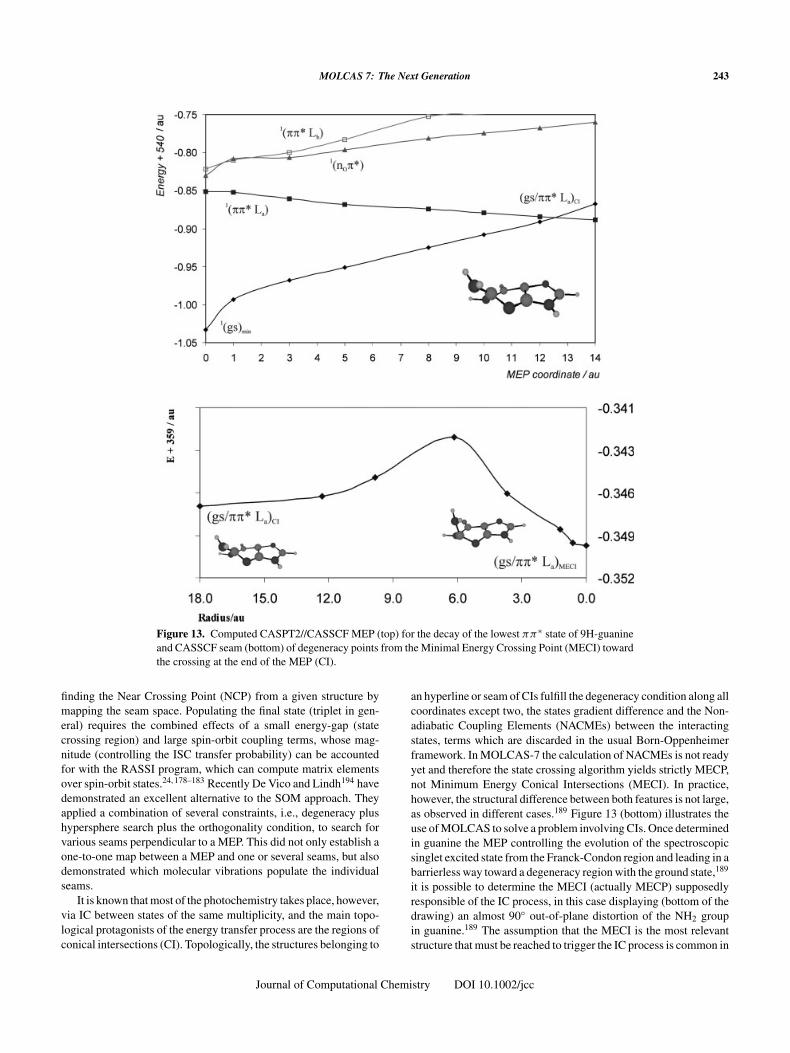
MOLCAS 7: The Next Generation 243
Figure 13. Computed CASPT2//CASSCF MEP (top) for the decay of the lowest ππ∗ state of 9H-guanineand CASSCF seam (bottom) of degeneracy points from the Minimal Energy Crossing Point (MECI) towardthe crossing at the end of the MEP (CI).
finding the Near Crossing Point (NCP) from a given structure bymapping the seam space. Populating the final state (triplet in gen-eral) requires the combined effects of a small energy-gap (statecrossing region) and large spin-orbit coupling terms, whose mag-nitude (controlling the ISC transfer probability) can be accountedfor with the RASSI program, which can compute matrix elementsover spin-orbit states.24, 178–183 Recently De Vico and Lindh194 havedemonstrated an excellent alternative to the SOM approach. Theyapplied a combination of several constraints, i.e., degeneracy plushypersphere search plus the orthogonality condition, to search forvarious seams perpendicular to a MEP. This did not only establish aone-to-one map between a MEP and one or several seams, but alsodemonstrated which molecular vibrations populate the individualseams.
It is known that most of the photochemistry takes place, however,via IC between states of the same multiplicity, and the main topo-logical protagonists of the energy transfer process are the regions ofconical intersections (CI). Topologically, the structures belonging to
an hyperline or seam of CIs fulfill the degeneracy condition along allcoordinates except two, the states gradient difference and the Non-adiabatic Coupling Elements (NACMEs) between the interactingstates, terms which are discarded in the usual Born-Oppenheimerframework. In MOLCAS-7 the calculation of NACMEs is not readyyet and therefore the state crossing algorithm yields strictly MECP,not Minimum Energy Conical Intersections (MECI). In practice,however, the structural difference between both features is not large,as observed in different cases.189 Figure 13 (bottom) illustrates theuse of MOLCAS to solve a problem involving CIs. Once determinedin guanine the MEP controlling the evolution of the spectroscopicsinglet excited state from the Franck-Condon region and leading in abarrierless way toward a degeneracy region with the ground state,189
it is possible to determine the MECI (actually MECP) supposedlyresponsible of the IC process, in this case displaying (bottom of thedrawing) an almost 90◦ out-of-plane distortion of the NH2 groupin guanine.189 The assumption that the MECI is the most relevantstructure that must be reached to trigger the IC process is common in
Journal of Computational Chemistry DOI 10.1002/jcc
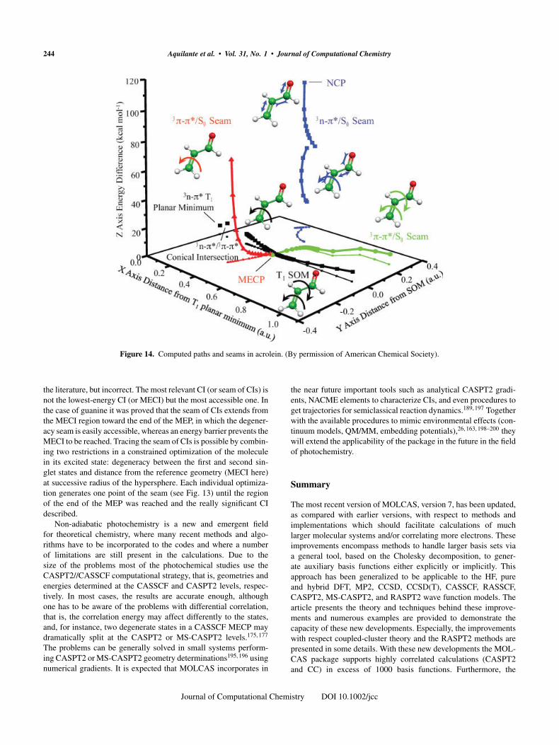
244 Aquilante et al. • Vol. 31, No. 1 • Journal of Computational Chemistry
Figure 14. Computed paths and seams in acrolein. (By permission of American Chemical Society).
the literature, but incorrect. The most relevant CI (or seam of CIs) isnot the lowest-energy CI (or MECI) but the most accessible one. Inthe case of guanine it was proved that the seam of CIs extends fromthe MECI region toward the end of the MEP, in which the degener-acy seam is easily accessible, whereas an energy barrier prevents theMECI to be reached. Tracing the seam of CIs is possible by combin-ing two restrictions in a constrained optimization of the moleculein its excited state: degeneracy between the first and second sin-glet states and distance from the reference geometry (MECI here)at successive radius of the hypersphere. Each individual optimiza-tion generates one point of the seam (see Fig. 13) until the regionof the end of the MEP was reached and the really significant CIdescribed.
Non-adiabatic photochemistry is a new and emergent fieldfor theoretical chemistry, where many recent methods and algo-rithms have to be incorporated to the codes and where a numberof limitations are still present in the calculations. Due to thesize of the problems most of the photochemical studies use theCASPT2//CASSCF computational strategy, that is, geometries andenergies determined at the CASSCF and CASPT2 levels, respec-tively. In most cases, the results are accurate enough, althoughone has to be aware of the problems with differential correlation,that is, the correlation energy may affect differently to the states,and, for instance, two degenerate states in a CASSCF MECP maydramatically split at the CASPT2 or MS-CASPT2 levels.175, 177
The problems can be generally solved in small systems perform-ing CASPT2 or MS-CASPT2 geometry determinations195, 196 usingnumerical gradients. It is expected that MOLCAS incorporates in
the near future important tools such as analytical CASPT2 gradi-ents, NACME elements to characterize CIs, and even procedures toget trajectories for semiclassical reaction dynamics.189, 197 Togetherwith the available procedures to mimic environmental effects (con-tinuum models, QM/MM, embedding potentials),26, 163, 198–200 theywill extend the applicability of the package in the future in the fieldof photochemistry.
Summary
The most recent version of MOLCAS, version 7, has been updated,as compared with earlier versions, with respect to methods andimplementations which should facilitate calculations of muchlarger molecular systems and/or correlating more electrons. Theseimprovements encompass methods to handle larger basis sets viaa general tool, based on the Cholesky decomposition, to gener-ate auxiliary basis functions either explicitly or implicitly. Thisapproach has been generalized to be applicable to the HF, pureand hybrid DFT, MP2, CCSD, CCSD(T), CASSCF, RASSCF,CASPT2, MS-CASPT2, and RASPT2 wave function models. Thearticle presents the theory and techniques behind these improve-ments and numerous examples are provided to demonstrate thecapacity of these new developments. Especially, the improvementswith respect coupled-cluster theory and the RASPT2 methods arepresented in some details. With these new developments the MOL-CAS package supports highly correlated calculations (CASPT2and CC) in excess of 1000 basis functions. Furthermore, the
Journal of Computational Chemistry DOI 10.1002/jcc
MOLCAS 7: The Next Generation 245
MOLCAS package has been improved with respect to the applicabil-ity of the one-component wave functions models to address chemicalproblems involving elements of the whole periodic table. In particu-lar, the paper demonstrates the benefits of the so-called ANO-RCCbasis set library covering all elements and presents the theoryand implementation of the picture-change-free property integralsto be used in association with relativistic calculations originatingfrom the DKH transformation. The ESPF QM/MM interface, theMOLCAS/Tinker implementation, which in principle can han-dle any kind of MM forcefield, is presented and discussed. Themanuscript is concluded with a section, which in some details,describes the usefulness of the MOLCAS package in associationwith the study of photochemistry. More specifically, the implemen-tation of constrained geometry optimization to facilitate the searchfor MEPs, MECPs, ISCs, and CIs are discussed as well as the anal-ysis of the relationship between reaction paths and seams of variousnature. This section is supported by illustrative examples.
Acknowledgments
N.F. thanks M. Olivucci for the figure illustrating the QM/MMsection.
References
1. Lindh, R.; Malmqvist, P.-Å. Theor Chem Acc 2003, 110, 115.2. Roos, B. Chem Phys Lett 1972, 15, 153.3. Siegbahn, P. E. M. In Current Aspects of Quantum Chemistry 1981:
Proceedings of an International Conference and Workshop, Barcelona,Spain, 28 September – 3 October 1981; Carbó, R., Ed.; ElsevierScientific Publishing Company: Amsterdam, 1987; p 65.
4. Roos, B. O.; Taylor, P. R.; Siegbahn, P. E. M. Chem Phys 1980, 48,157.
5. Siegbahn, P. E. M.; Almlöf, J.; Heiberg, J.; Roos, B. O. J Chem Phys1981, 74, 2384.
6. Roos, B. O. Int J Quantum Chem 1980, S14, 175.7. Roos, B.; Veillard, A.; Vinot, G. Theor Chim Acta 1971, 20, 1.8. Roos, B.; Siegbahn, P. Theor Chim Acta 1970, 17, 209.9. Roos, B.; Siegbahn, P. Theor Chim Acta 1970, 17, 199.
10. Andersson, K.; Malmqvist, P.-Å.; Roos, B. O.; Sadlej, A. J.; Wolinski,K. J Phys Chem 1990, 94, 5483.
11. Andersson, K.; Malmqvist, P.-Å.; Roos, B. O. J Chem Phys 1992, 96,1218.
12. Andersson, K.; Roos, B. O. In Modern Electron Structure TheoryAdvanced Series in Physical Chemistry, Vol. 2, Part I; Yarkony, R.,Ed.; World Scientific Publishing Co. Pte. Ltd.: Singapore, 1995; pp.55.
13. Finley, J.; Malmqvist, P.-Å.; Roos, B. O.; Serrano-Andrés, L. ChemPhys Lett 1998, 288, 299.
14. Lindh, R.; Ryu, U.; Liu, B. J Chem Phys 1991, 95, 5889.15. Ryu, U.; Lee, Y. S.; Lindh, R. Chem Phys Lett 1991, 185, 562.16. Lindh, R. Theor Chim Acta 1993, 85, 423.17. Stålring, J.; Bernhardsson, A.; Lindh, R. Mol Phys 2001, 99, 103.18. Lindh, R.; Bernhardsson, A.; Karlström, G.; Malmqvist, P.-Å. Chem
Phys Lett 1995, 241, 423.19. Lindh, R.; Bernhardsson, A.; Schütz, M. Chem Phys Lett 1999, 303,
567.20. Bernhardsson, A.; Lindh, R.; Olsen, J.; Fülscher, M. Mol Phys 1999,
96, 617.21. Olsen, J.; Roos, B. O.; Jørgensen, P.; Jensen, H. J. A. J Chem Phys
1988, 89, 2185.
22. Malmqvist, P.-Å.; Rendell, A.; Roos, B. O. J Phys Chem 1990, 94,5477.
23. Malmqvist, P. Å.; Roos, B. O. Chem Phys Lett 1989, 155, 189.24. Malmqvist, P.-Å.; Roos, B. O.; Schimmelpfennig, B. Chem Phys Lett
2002, 357, 230.25. Neogrády, P.; Pitonák, M.; Urban, M. Mol Phys 2005, 103, 2141.26. Karlström, G.; Lindh, R.; Malmqvist, P.-Å.; Roos, B. O.; Ryde,
U.; Veryazov, V.; Widmark, P.-O.; Cossi, M.; Schimmelpfennig, B.;Neogrády, P.; Seijo, L. Comput Mater Sci 2003, 28, 222.
27. Veryazov, V.; Widmark, P.-O.; Serrano-Andrés, L.; Lindh, R.; Roos,B. O. Int J Quantum Chem 2004, 100, 626.
28. Benoit, C. E. Bull Geodesique 1924, 7, 67.29. Golub, G. H.; Van Loan, C. F. Matrix Computations, 3rd Edition; Johns
Hopkins University Press: Baltimore, 1996.30. Beebe, N. H. F.; Linderberg, J. Int J Quantum Chem 1977, 12, 683.31. Koch, H.; Sánchez de Merás, A.; Pedersen, T. B. J Chem Phys 2003,
118, 9481.32. Pedersen, T. B.; Sánchez de Merás, A. M. J.; Koch, H. J Chem Phys
2004, 120, 8887.33. Whitten, J. L. J Chem Phys 1973, 58, 4496.34. Baerends, E. J.; Ellis, D. E.; Ros, P. Chem Phys 1973, 2, 41.35. Dunlap, B. I.; Connolly, J. W. D.; Sabin, J. R. J Chem Phys 1979, 71,
3396.36. Dunlap, B. I.; Connolly, J. W. D.; Sabin, J. R. J Chem Phys 1979, 71,
4993.37. Feyereisen, M.; Fitzgerald, G.; Komornicki, A. Chem Phys 1993, 208,
359.38. Vahtras, O.; Almlöf, J.; Feyereisen, M. W. Chem Phys Lett 1993, 213,
514.39. Aquilante, F.; Lindh, R.; Pedersen, T. B. J Chem Phys 2007, 127,
114107.40. Aquilante, F.; Pedersen, T. B.; Sánchez de Merás, A.; Koch, H. J Chem
Phys 2006, 125, Art. No 174101.41. Aquilante, F.; Pedersen, T. B.; Lindh, R. J Chem Phys 2007, 126, Art.
No 194106.42. Aquilante, F.; Pedersen, T. B. Chem Phys Lett 2007, 449, 354.43. Aquilante, F.; Lindh, R.; Pedersen, T. B. J Chem Phys 2008, 129, Art.
No 034106.44. Aquilante, F.; Pedersen, T. B.; Roos, B. O.; Sánchez de Merás, A.;
Koch, H. J Chem Phys 2008, 129, Art. No 024113.45. Aquilante, F.; Malmqvist, P.-Å.; Pedersen, T. B.; Ghosh, A.; Roos,
B. O. J Chem Theory Comput 2008, 4, 694.46. Aquilante, F.; Gagliardi, L.; Pedersen, T. B.; Lindh, R. J Chem Phys
2009, 130, 154107.47. Boström, J.; Aquilante, F.; Pedersen, T. B.; Lindh, R. J Chem Theory
Comput 2009, in press. DOI:10.1021/ct9000284.48. Pierloot, K.; Vancoillie, S. J Chem Phys 2008, 128, Art. No 034104.49. Radon, M.; Pierloot, K. J Phys Chem A 2008, 112, 11824.50. Widmark, P.-O.; Malmqvist, P.-Å.; Roos, B. O. Theor Chim Acta 1990,
77, 291.51. Widmark, P.-O.; Persson, B. J.; Roos, B. O. Theor Chim Acta 1991,
79, 419.52. Pou-Amérigo, R.; Merchán, M. Nebot-Gil, I.; Widmark, P.-O.; Roos,
B. O. Theor Chim Acta 1995, 92, 149.53. Pierloot, K.; Dumez, B.; Widmark, P.-O.; Roos, B. O. Theor Chim
Acta 1995, 90, 87.54. Roos, B. O.; Andersson, K.; Fülscher, M. P.; Malmqvist, P.-Å.;
Serrano-Andrés, L.; Pierloot, K.; Merchán, M. In Advances in Chem-ical Physics: New Methods in Computational Quantum Mechanics;Prigogine, I.; Rice, S. A., Eds.; Vol. XCIII:219–331, Wiley: New York,1996; p. 219.
55. Roos, B. O.; Veryazov, V.; Widmark, P.-O. Theor Chem Acc 2004,111, 345.
Journal of Computational Chemistry DOI 10.1002/jcc
246 Aquilante et al. • Vol. 31, No. 1 • Journal of Computational Chemistry
56. Roos, B. O.; Lindh, R.; Malmqvist, P.-Å.; Veryazov, V.; Widmark, P.-O.J Phys Chem A 2004, 108, 2851.
57. Roos, B. O.; Lindh, R.; Malmqvist, P.-Å.; Veryazov, V.; Widmark, P.-O.J Phys Chem A 2005, 109, 6575.
58. Roos, B. O.; Lindh, R.; Malmqvist, P.-Å.; Veryazov, V.; Widmark, P.-O.Chem Phys Lett 2005, 409, 295.
59. Roos, B. O.; Lindh, R.; Malmqvist, P.-Å.; Veryazov, V.; Widmark,P.-O.; Borin, A. C. J Phys Chem A 2008, 112, 11431.
60. Faegri K., Jr. Theor Chem Acc 2001, 105, 252.61. Sansonetti, J.; Martin, W.; Young, S. Handbook of Basic
Atomic Spectroscopic Data (version 1.00); [Online] Available at:http://physics.nist.gov/Handbook; National Institute of Standards andTechnology: Gaithersburg, MD, 2003.
62. Lide D. R., Ed. Handbook of Chemistry and Physics; CRC Press: BocaRaton, 2002.
63. Reiher, M.; Wolf, A. Relativistic Quantum Chemistry; Wiley-VCH:Weinheim, 2009.
64. Roos, B. O.; Malmqvist, P.-Å.; Gagliardi, L. In Fundamental World ofQuantum Chemistry; Brändas, E.; Kryachko, E., Eds.; Kluwer Acad.Publ.: Dordrecht, The Netherlands, 2003; p. 425.
65. Roos, B. O.; Malmqvist, P.-Å. Adv Quantum Chem 2004, 47, 37.66. Gagliardi, L.; Roos, B. O. Chem Soc Rev 2007, 36, 893.67. Douglas, M.; Kroll, N. M. Ann Phys 1974, 82, 89.68. Hess, B. A. Phys Rev A 1986, 33, 3742.69. Reiher, M.; Wolf, A. J Chem Phys 2004, 121, 2037.70. Wolf, A.; Reiher, M.; Hess, B. A. J Chem Phys 2002, 117, 9215.71. Reiher, M.; Wolf, A. Phys Lett A 2007, 360, 603.72. Reiher, M.; Wolf, A. J Chem Phys 2004, 121, 10945.73. Reiher, M. Theor Chem Acc 2006, 116, 241.74. Baerends, E. J.; Schwarz, W. H. E.; Schwerdtfeger, P.; Snijders, J. G.
J Phys B 1990, 23, 3225.75. Kellö, V.; Sadlej, A. J. Int J Quantum Chem 1998, 68, 159.76. Wolf, A.; Reiher, M. J Chem Phys 2006, 124, Art. No 064102.77. Wolf, A.; Reiher, M. J Chem Phys 2006, 124, Art No 064103.78. Mastalerz, R.; Barone, G.; Lindh, R.; Reiher, M. J Chem Phys 2007,
127, Art. No 074105.79. Luber, S.; Ondík, I. M.; Reiher, M. Chem Phys 2009, 356, 205.80. Mastalerz, R.; Lindh, R.; Reiher, M. Chem Phys Lett 2008, 465, 157.81. Barone, G.; Mastalerz, R.; Lindh, R.; Reiher, M. J Phys Chem A 2008,
112, 1666.82. Chan, G. K.-L.; Dorando, J. J.; Gosh, D.; Hachmann, J.; Neuscamman,
E.; Wang, H.; Yanai, T. In Frontiers in Quantum Systems in Chemistryand Physics, Vol. 18; Wilson, S.; Grout, P. J.; Maruani, J.; Delgado-Barrio, G.; Piecuch, P., Eds.; Springer: Dordrecht, Netherlands, 2008;p. 49.
83. Marti, K. H.; Ondík, I. M.; Moritz, G.; Reiher, M. J Chem Phys 2008,128, Art. No. 014104.
84. Ghosh, D.; Hachmann, J.; Yanai, T.; Chan, G. K.-L. J Chem Phys 2008,128, Art. No. 144117.
85. Celani, P.; Stoll, H.; Werner, H.; Knowles, P. Mol Phys 2004, 102,2369.
86. Angeli, C.; Pastore, M.; Cimiraglia, R. Theor Chim Acta 2007, 117,743.
87. Gagliardi, L.; Roos, B. O. Nature 2005, 433, 848.88. Gagliardi, L.; Heaven, M. C.; Krogh, J. W.; Roos, B. O. J Am Chem
Soc 2005, 127, 86.89. Gagliardi, L.; Pyykkö, P.; Roos, B. O. Phys Chem Chem Phys 2005,
7, 2415.90. Gagliardi, L.; Roos, B. O. In Trends and Perspectives in Modern Com-
putational Science (ICCMSE06); Maroulis, G.; Simos T., Eds.; BrillAcademic Publishers: The Netherlands, 2006; Ch. 2, p. 23.
91. LaMacchia, G.; Brynda, G. M.; Gagliardi, L. Angew Chem Int Ed Eng2006, 45, 6210.
92. Roos, B. O.; Gagliardi, L. Inorg Chem 2006, 45, 803.
93. Ghosh, A.; Gonzalez, E.; Tangen, E.; Roos, B. O. J Phys Chem A 2008,112, 12792.
94. Schreiber, M.; Silva, M. R., Jr.; Sauer, S. P. A.; Thiel, W. J Chem Phys2008, 128, Art. No 134110.
95. Celani, P.; Werner, H.-J. J Chem Phys 2000, 112, 5546.96. Malmqvist, P.-Å.; Pierloot, K.; Shahi, A. R. M.; Cramer, C. J.;
Gagliardi, L. J Chem Phys 2008, 128, Art. No 204109.97. Cížek, J. J Chem Phys 1966, 45, 4256.98. Paldus, J.; Li, X. Z. Adv Chem Phys 1999, 110, 1.99. Bartlett, R. J. In Advanced Series in Physical Chemistry, Vol. 2;
Yarkony, D. R., Ed.; World Scientific: Singapore, 1995; p. 1047.100. Urban, M.; Cernušák, I.; Noga, J.; Kellö, V. In Methods in Compu-
tational Chemistry, Vol. 1; Wilson, S., Ed.; Plenum Press: New York,1987; p. 117.
101. Gauss, J.; Schleyer, P. v. R., Ed. Encyclopedia of ComputationalChemistry; Wiley: Chichester, 1998; p. 615.
102. Bartlett, R. J.; Musial, M.; Rev Mod Phys 2007, 79, 291.103. Li, X. Z.; Paldus, J. J Chem Phys 1997, 107, 6257.104. Pittner, J.; Šmydke, J.; Cársky, P.; Hubac, I. Theochem-J Mol Struct
2001, 547, 239.105. Musial, M.; Kucharski, S. A.; Bartlett, R. J. J Chem Phys 2002, 116,
4382.106. Piecuch, P.; Kucharski, S. A.; Bartlett, R. J. J Chem Phys 1999, 110,
6103.107. Chattopadhyay, S.; Pahari, D.; Mukherjee, D.; Mahapatra, U. S. J Chem
Phys 2004, 120, 5968.108. Raghavachari, K.; Trucks, G. W.; Pople, J. A.; Head-Gordon, M. Chem
Phys Lett 1989, 157, 479.109. Urban, M.; Noga, J.; Cole, S. J.; Bartlett, R. J. J Chem Phys 1985, 83,
4041.110. Noga, J.; Bartlett, R. J. J Chem Phys 1987, 86, 7041.111. Noga, J.; Bartlett, R. J.; Urban, M. Chem Phys Lett 1987, 134, 126.112. Li, X. Z.; Paldus, J. J Chem Phys 1994, 101, 8812.113. Kallay, M.; Surjan, P. R. J Chem Phys 2001, 115, 2945.114. Neogrády, P.; Szalay, P. G.; Kraemer, W. P.; Urban, M. Collect Czech
Chem Commun 2005, 70, 951.115. Stanton, J. F.; Gauss, J.; Watts, J. D.; Bartlett, R. J. J Chem Phys 1991,
94, 4334.116. Urban, M.; Neogrády, P.; Hubac, I. In Recent Advances in Com-
putational Chemistry, Vol. 3; Bartlett, R. J., Ed.; World Scientific:Singapore, 1997; p. 275.
117. Neogrády, P.; Urban, M. Int J Quantum Chem 1995, 55, 187.118. Watts, J. D.; Gauss, J.; Bartlett, R. J. J Chem Phys 1993, 98, 8718.119. Takahashi, M.; Paldus, J. J Chem Phys 1986, 85, 1486.120. Heckert, M.; Heun, O.; Gauss, J.; Szalay, P. G. J Chem Phys 2006, 124,
Art No 124105.121. Koch, H.; deMeras, A. S.; Helgaker, T.; Christiansen, O. J Chem Phys
1996, 104, 4157.122. Noga, J.; Valiron, P. Mol Phys 2005, 103, 2123.123. Constans, P.; Ayala, P. Y.; Scuseria, G. E. J Chem Phys 2000, 113,
10451.124. Olson, R. M.; Bentz, J. L.; Kendall, R. A.; Schmidt, M. W.; Gordon,
M. S. J Chem Theory Comput 2007, 3, 1312.125. Janowski, T.; Ford, A. R.; Pulay, P. J Chem Theory Comput 2007, 3,
1368.126. Janowski, T.; Pulay, P. J Chem Theory Comput 2008, 4, 1585.127. Lotrich, V.; Flocke, N.; Ponton, M.; Yau, A. D.; Perera, A.; Deumens,
E.; Bartlett, R. J. J Chem Phys 2008, 128, Art. No 194104.128. Koch, H.; de Meras, A. S. J Chem Phys 2000, 113, 508.129. Constans, P.; Scuseria, G. E. Collect Czech Chem Commun 2003, 68,
357.130. Maslen, P. E.; Dutoi, A. D.; Lee, M. S.; Shao, Y. H.; Head-Gordon, M.
Mol Phys 2005, 103, 425.131. Adamowicz, L.; Bartlett, R. J. J Chem Phys 1987, 86, 6314.
Journal of Computational Chemistry DOI 10.1002/jcc
MOLCAS 7: The Next Generation 247
132. Adamowicz, L.; Bartlett, R. J.; Sadlej, A. J. J Chem Phys 1988, 88,5749.
133. Pitonák, M.; Neogrády, P.; Kellö, V.; Urban, M. Mol Phys 2006, 104,2277.
134. Dedíková, P.; Pitonák, M.; Neogrády, P.; Rezác, I.; Urban, M. J PhysChem A 2008, 112, 7115.
135. Šulka, M.; Pitonák, M.; Neogrády, P.; Urban, M. Int J Quantum Chem2008, 108, 2159.
136. Boman, L.; Koch, H. Int J Quantum Chem 2009, 109, 708.137. Taube, A. G.; Bartlett, R. J. Collect Czech Chem Commun 2005, 70,
837.138. Taube, A. G.; Bartlett, R. J. J Chem Phys 2008, 128, Art. No 164101.139. Noga, J.; Kutzelnigg, W. J Chem Phys 1994, 101, 7738.140. Laidig, W. D.; Purvis, G. D.; Bartlett, R. J. J Phys Chem 1985, 89,
2161.141. Schütz, M.; Werner, H. J. J Chem Phys 2001, 114, 661.142. Korona, T.; Pflüger, K.; Werner, H. J. Phys Chem Chem Phys 2004, 6,
2059.143. Pitonák, M.; Neogrády, P.; Rezác, J.; Jurecka, P.; Urban, M.; Hobza,
P. J Chem Theory Comput 2008, 4, 1829.144. Pitonák, M.; Riley, K. E.; Neogrády, P.; Hobza, P. Chem Phys Chem
2008, 9, 1636.145. Dunning, T. H.; Peterson, K. A.; Woon, D. E. In Encyclopedia of
Computational Chemistry; Schleyer, P. v. R., Ed.; Wiley: Chichester,1998; p. 88.
146. Neogrády, P.; Medved, M.; Cernušák, I.; Urban, M. Mol Phys 2002,100, 541.
147. Ervin, K. M.; Anusiewicz, I.; Skurski, P.; Simons, J.; Lineberger, W. C.J Phys Chem A 2003, 107, 8521.
148. González-Luque, R.; Merchán, M.; Fülscher, M. P.; Roos, B. O. ChemPhys Lett 1993, 204, 323.
149. Bachorz, R. A.; Klopper, W.; Gutowski, M. J Chem Phys 2007, 126,Art. No 085101.
150. Bachorz, R. A.; Klopper, W.; Gutowski, M.; Li, X.; Bowen, K. H.J Chem Phys 2007, 129, Art. No 054309.
151. Roca-Sanjuan, D.; Merchán, M.; Serrano-Andrés, L.; Rubio, M.J Chem Phys 2008, 129, Art No 095104.
152. Karlström, G. J Phys Chem 1988, 92, 1315.153. Cossi, M.; Rega, N.; Scalmani, G.; Barone, V. J Chem Phys 2001, 114,
5691.154. Barandiarán, Z.; Seijo, L. J Chem Phys 1988, 89, 5739.155. Warshel, A.; Levitt, M. J Mol Biol 1976, 103, 227.156. Field, M. J.; Bash, P. A.; Karplus, M. J Comp Chem 1990, 11, 700.157. Lin, H.; Truhlar, D. G. Theor Chem Acc 2006, 117, 185.158. Ferré, N.; Ángyán, J. G. Chem Phys Lett 2002, 356, 331.159. Ponder, J. W. Tinker4.2—software tools for molecular design; Avail-
able at: http://dasher.wustl.edu/tinker; 2004.160. Vreven, T.; Morokuma, K.; Farkas, O.; Schlegel, H. B.; Frisch, M. J.
J Comput Chem 2003, 24, 760.161. Coto, P. B.; Strambi, A.; Ferré, N.; Olivucci, M. Proc Natl Acad Sci
USA 2006, 103, 17154.162. Frutos, L. M.; Andruniów, T.; Santoro, F.; Ferré, N.; Olivucci, M. Proc
Natl Acad Sci USA 2007, 104, 7764.163. Strambi, A.; Coto, P. B.; Frutos, L. M.; Ferré, N.; Olivucci, M. J Am
Chem Soc 2008, 130, 3382.164. Roca-Sanjuán, D.; Olaso-González, G.; Rubio, M.; Brana-Coto, P.;
Merchán, M.; Ferré, N.; Ludwig, V.; Serrano-Andrés, L. Pure ApplChem 2009, 81, 743.
165. Olivucci, M., Ed. Computational Photochemistry; Elsevier: Amster-dam, 2005.
166. Roos, B. O.; Fülscher, M. P.; Malmqvist, P.-Å.; Merchán, M.; Serrano-Andrés, L. In Quantum Mechanical Electronic Structure Calculationswith Chemical Accuracy; Langhoff, S. R., Ed.; Kluwer Academic
Publishers, Understanding Chem. React.: Dordrecht, The Netherlands,1995; p. 357.
167. Merchán, M.; Serrano-Andrés, L.; Fülscher, M. P.; Roos, B. O. InRecent Advances in Multireference Theory, Vol. IV; K. H. U., Ed.;World Scientific Publishing Co, Pte. Ltd: Singapore, 1999; p. 161.
168. Serrano-Andrés, L.; Forsberg, N.; Malmqvist, P.-Å. J Chem Phys 1998,108, 7202.
169. Bernhardsson, A.; Forsberg, N.; Malmqvist, P.-Å.; Roos, B. O.;Serrano-Andrés, L. J Chem Phys 2000, 112, 2798.
170. Pou-Amérigo, R.; Serrano-Andrés, L.; Merchán, M.; Ortí, E.; Forsberg,N. J Am Chem Soc 2000, 122, 6067.
171. Roos, B. O.; Malmqvist, P.-Å.; Molina, V.; Serrano-Andrés, L.;Merchán, M. J Chem Phys 2002, 116, 7526.
172. Serrano-Andrés, L.; Merchán, M. Chem Phys Lett 2006, 418, 569.173. De Vico, L.; Lindh, R.; Olivucci, M. J Chem Theory Comput 2005, 1,
1029.174. Pierloot, K. Mol Phys 2003, 101, 2083.175. Serrano-Andrés, L.; Merchán, M. J Mol Struct Theochem 2005, 729,
99.176. Pérez-Hernández, G.; González, L.; Serrano-Andrés, L. Chem Phys
Chem 2008, 9, 2544.177. Serrano-Andrés, L.; Merchán, M.; Lindh, R. J Chem Phys 2005, 122,
Art. No 104106.178. Climent, T.; González-Luque, R.; Merchán, M.; Serrano-Andrés, L.
Chem Phys Lett 2007, 441, 327.179. Serrano-Pérez, J. J.; González-Luque, R.; Merchán, M.; Serrano-
Andrés, L. J Phys Chem B 2007, 111, 11880.180. Merchán, M.; Serrano-Andrés, L.; Robb, M. A.; Blancafort, L. J Am
Chem Soc 2005, 127, 1820.181. Climent, T.; González-Luque, R.; Merchán, M.; Serrano-Andrés, L.
J Phys Chem A 2006, 110, 13584.182. Serrano-Pérez, J. J.; Serrano-Andrés, L.; Merchán, M. J Chem Phys
2006, 124, Art. No 124502.183. Liu, Y.-J.; De Vico, L.; Lindh, R.; Fang, W.-H. Chem Phys Chem 2007,
8, 890.184. Serrano-Andrés, L.; Sánchez-Marín, J.; Nebot-Gil, I. J Chem Phys
1992, 97, 7499.185. Serrano-Andrés, L.; Merchán, M.; Nebot-Gil, I.; Lindh, R.; Roos, B. O.
J Chem Phys 1993, 98, 3151.186. Serrano-Andrés, L.; Lindh, R.; Roos, B. O.; Merchán, M. J Phys Chem
1993, 97, 9360.187. Anglada, J. M. Bofill, J. M. J Comput Chem 1997, 18, 992.188. Müller, K.; Brown, L. D.; Theor Chim Acta 1979, 53, 75.189. Serrano-Andrés, L.; Merchán, M.; Borin, A. C. J Am Chem Soc 2008,
130, 2473.190. Merchán, M.; González-Luque, R.; Climent, T.; Serrano-Andrés, L.;
Rodríguez, E.; Reguero, M.; Peláez, D. J Phys Chem B 2006, 110,26471.
191. Serrano-Andrés, L.; Merchán, M.; Borin, A. C. Proc Natl Acad SciUSA 2006, 103, 8691.
192. Serrano-Andrés, L.; Merchán, M.; Borin, A. C. Chem Eur J 2006, 12,6559.
193. Serrano-Andrés, L.; Merchán, M. J Photochem Photobiol C (in press).194. De Vico, L.; Lindh, R. J Chem Theory Comput 2009, 5, 186.195. De Vico, L.; Wisborg-Krogh, J.; Liu, Y.-J.; Lindh, R. J Phys Chem A
2007, 111, 8013.196. De Vico, L.; Pegado L.; Heimdal, J.; Söderhjelm, P.; Roos, B. O. Chem
Phys Lett 2008, 461, 136.197. Weingart, O.; Shapiro, I.; Buss, V. J Phys Chem B 2007, 111, 3782.198. Serrano-Andrés, L.; Fülscher, M. P.; Karlström, G. Int J Quantum
Chem 1997, 65, 167.199. Proppe, B.; Merchán, M.; Serrano-Andrés, L. J Phys Chem A 2000,
104, 1608.200. Seijo, L.; Barandiarán, Z. In Computational Chemistry: Reviews
of Current Trends, Vol. 4; Leszczynski, J., Ed.; World Scientific:Singapur; 1999; p. 55.
Journal of Computational Chemistry DOI 10.1002/jcc