module exponential and logarithmic functions 1 b5 – exponential and logarithmic functions 5.1...
TRANSCRIPT
Module B5 – Exponential and logarithmic functions
Module B5
Exponential and logarithmic functions 1
Table of Contents
Introduction ................................................................................................................. 5.1
5.1 Exponential functions ......................................................................................... 5.2 5.1.1 The function and its graph ............................................................................. 5.2 5.1.2 The exponential function ............................................................................... 5.9 5.1.3 Case studies ................................................................................................... 5.9
Population growth ................................................................................................. 5.9 Compound interest .............................................................................................. 5.10 Depreciation ........................................................................................................ 5.13 Chemical reactions .............................................................................................. 5.14
5.1.4 Average rate of change ................................................................................ 5.19 5.1.5 The inverse of the exponential function ...................................................... 5.24
5.2 Logarithmic functions ....................................................................................... 5.27 5.2.1 What is a logarithm? ................................................................................... 5.27 5.2.2 Properties of logarithms .............................................................................. 5.32 5.2.3 The function and its graph ........................................................................... 5.37 5.2.4 Case studies ................................................................................................. 5.38
Measuring loudness ............................................................................................ 5.39 Measuring acidity ............................................................................................... 5.40
5.2.5 Average rate of change ................................................................................ 5.42
5.3 Putting it all together – solving equations and real world applications .............. 5.43 Real world applications ...................................................................................... 5.47
5.4 A taste of things to come .................................................................................. 5.50
5.5 Post-test ............................................................................................................ 5.52
5.6 Solutions ........................................................................................................... 5.55
Module B5 – Exponential and logarithmic functions 5.1
Introduction
Historians use it, banks use it, fish breeders use it, hospitals use it, even nuclear physicists use it. The exponential and its related function are often thought to be the most commonly occurring non-linear functions in nature. One type of exponential function is typified by its slow start followed by an ever increasing rise, while the other decreases quickly then slows down...if you have had the flu then you have experienced an exponential growth function in action. First by the rapid way the virus takes over your body, then when you take a painkiller how it rapidly relieves some of the symptoms for a while.
You will have previously studied exponential functions in Mathematics tertiary preparation level A or elsewhere. In this module we will refresh and build on this knowledge to develop a fuller understanding of the exponential function, its related function, the logarithmic function, and their uses.
More formally when you have successfully completed this module you should be able to:
• describe the pattern of exponential growth and decay in words, algebraic terms and using graphs
• recognize the occurrence of exponential growth and decay in real world situations
• demonstrate an understanding of the definition of a logarithm and its relationship to the exponential function
• use the logarithmic laws to simplify expressions and solve problems
• recognize the occurrence of logarithmic functions in real world situations
• solve problems involving exponential growth and decay, graphically and algebraically
• solve simple exponential equations.
5.2 TTPP7182 – Mathematics tertiary preparation level B
5.1 Exponential functions
5.1.1 The function and its graph
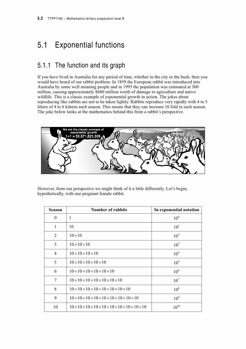
If you have lived in Australia for any period of time, whether in the city or the bush, then you would have heard of our rabbit problem. In 1859 the European rabbit was introduced into Australia by some well meaning people and in 1995 the population was estimated at 300 million, causing approximately $600 million worth of damage to agriculture and native wildlife. This is a classic example of exponential growth in action. The jokes about reproducing like rabbits are not to be taken lightly. Rabbits reproduce very rapidly with 4 to 5 litters of 4 to 6 kittens each season. This means that they can increase 10 fold in each season. The joke below looks at the mathematics behind this from a rabbit’s perspective.
However, from our perspective we might think of it a little differently. Let’s begin, hypothetically, with one pregnant female rabbit.
Season Number of rabbits In exponential notation
0 1
1 10
2
3
4
5
6
7
8
9
10
010
110
1010 210
101010 310
10101010 410
1010101010 510
101010101010 610
10101010101010 710
1010101010101010 810
101010101010101010 910
10101010101010101010 1010
Module B5 – Exponential and logarithmic functions 5.3
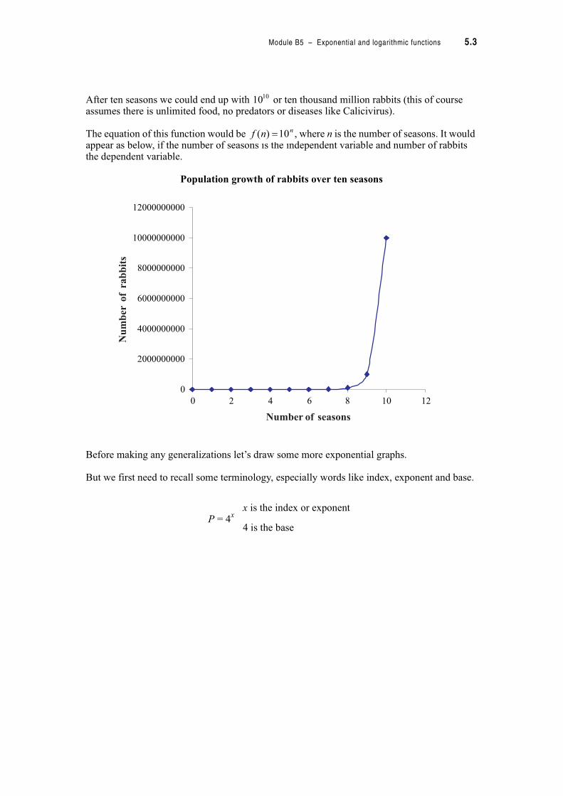
After ten seasons we could end up with or ten thousand million rabbits (this of course assumes there is unlimited food, no predators or diseases like Calicivirus).
The equation of this function would be , where n is the number of seasons. It would appear as below, if the number of seasons is the independent variable and number of rabbits the dependent variable.
Population growth of rabbits over ten seasons
Before making any generalizations let’s draw some more exponential graphs.
But we first need to recall some terminology, especially words like index, exponent and base.
P = 4x
x is the index or exponent
4 is the base
1010
nnf 10)( !
0
0 2 4 6 8 10 12
2000000000
4000000000
6000000000
8000000000
10000000000
12000000000
Num
ber
of
rabbits
Number of seasons

5.4 TTPP7182 – Mathematics tertiary preparation level B
Activity 5.1
1. Sketch the graph of
2. Sketch the graph of
After drawing these graphs think about the similarities between them and list them below.
__________________________________________________________________________
__________________________________________________________________________
__________________________________________________________________________
__________________________________________________________________________
Graphs which increase as the independent variable increases like the graphs in activity 5.1 are called exponential growth functions.
Other important characteristics of the graphs in activity 5.1 are that:
• they are all functions because there is only one value of the dependent variable for each value of the independent variable
• their domains are all unrestricted and include all real numbers
• the range of each function is restricted to values greater than zero
• the vertical intercept is one
• as the independent variable gets more negative (approaches negative infinity) the dependent variable gets closer and closer to zero
• as the independent variable increases (approaches infinity) the dependent variable increases very quickly.
Note, when a function gets very close to a value but does not reach it we say that we have an asymptote at that value. In this case the asymptote will be the straight line y = 0. So for exponential growth functions the horizontal axis is an asymptote.
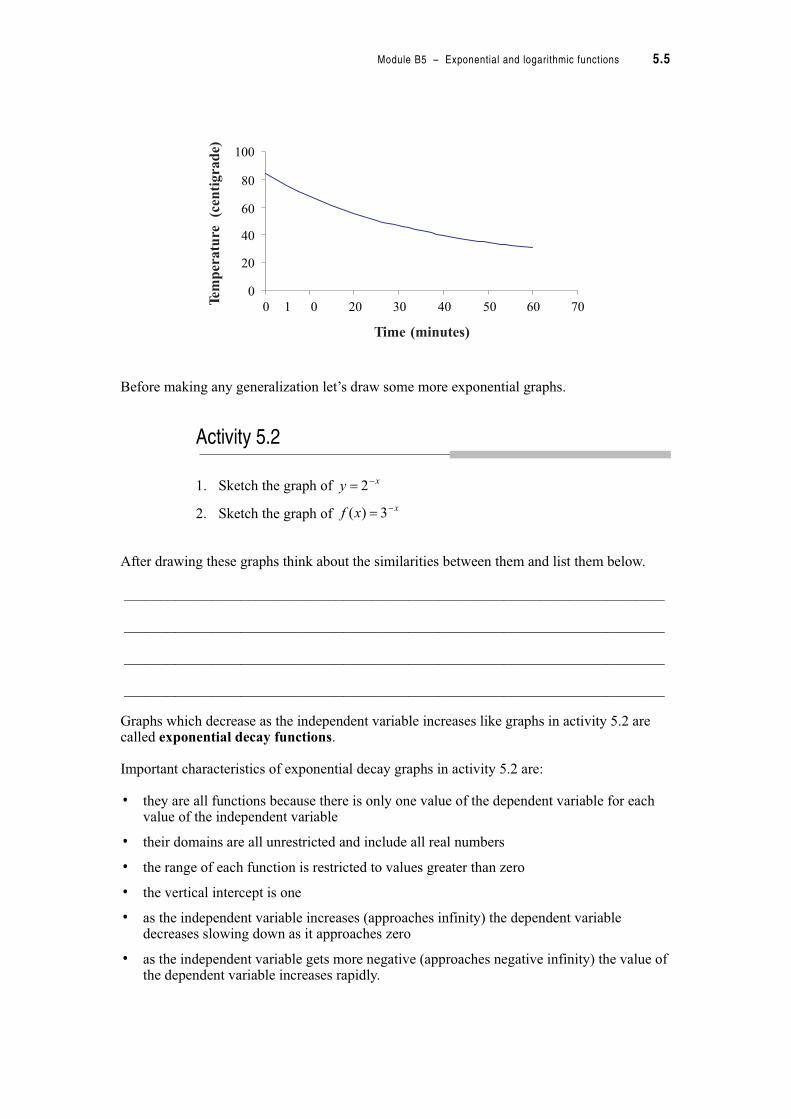
Not all exponential graphs represent growth functions. Have you ever wondered why that cup of coffee you thought you just poured got cold so quickly? Think about the graph below which represents the temperature of a cooling cup of coffee.
Temperature of a cup of coffee over time
xy 2!
xxf 3)( !
Module B5 – Exponential and logarithmic functions 5.5
Before making any generalization let’s draw some more exponential graphs.
Activity 5.2
1. Sketch the graph of
2. Sketch the graph of
After drawing these graphs think about the similarities between them and list them below.
__________________________________________________________________________
__________________________________________________________________________
__________________________________________________________________________
__________________________________________________________________________
Graphs which decrease as the independent variable increases like graphs in activity 5.2 are called exponential decay functions.
Important characteristics of exponential decay graphs in activity 5.2 are:
• they are all functions because there is only one value of the dependent variable for each value of the independent variable
• their domains are all unrestricted and include all real numbers
• the range of each function is restricted to values greater than zero
• the vertical intercept is one
• as the independent variable increases (approaches infinity) the dependent variable decreases slowing down as it approaches zero
• as the independent variable gets more negative (approaches negative infinity) the value of the dependent variable increases rapidly.
20
40
60
80
0
0 1 0 20 30 40 50 60 70
20
40
60
80
100
Tem
per
atu
re(c
entigra
de)
Time (minutes)
xy "! 2
xxf "! 3)(

5.6 TTPP7182 – Mathematics tertiary preparation level B
Note, for exponential decay functions the horizontal axis is an asymptote. In activity 5.2 the asymptote is y = 0.
As we can see from the discussion above there are many similarities between exponential graphs, but there are also a number of differences. Sketch the three graphs below either on a graphing package or by hand and think about the differences between the graphs.
You should have sketched something like this.
The differences you might have noticed are:
• Both and intersect the y-axis at y = 1, while intersects the axis at
y = 4
• increases at a rate faster than
• appears to increase at the same rate as , but is slower than .
Recall from module 3 that if you want to find the vertical intercept of a function you have to find the value when the horizontal variable is zero.
x
x
x
y
y
y
34
3
3
2
!
!
!
x
y
y = 3x
y = 4 3x
×
y = 32x
−4 −2 0 2 4
−5
5
xy 3! xy 23! xy 34 !
xy 23! xy 3!
xy 34 !xy 3! xy 23!
Module B5 – Exponential and logarithmic functions 5.7
Example
Find the y-intercept of .
To find the y-intercept we have to put t = 0
Activity 5.3
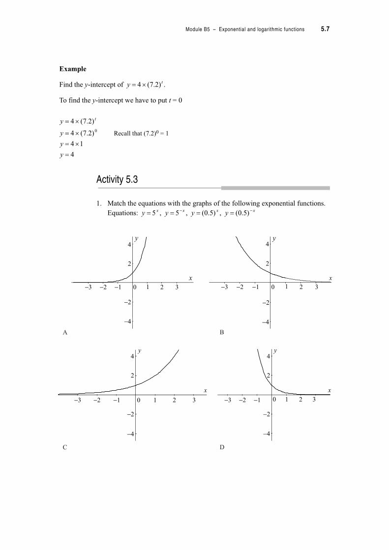
1. Match the equations with the graphs of the following exponential functions.
Equations:
Recall that (7.2)0 = 1
ty )2.7(4 !
4
14
)2.7(4
)2.7(4
0
!
!
!
!
y
y
y
y t
xxxx yyyy ""!!!! )5.0( ,)5.0( ,5 ,5
y
xx
y
−3 −2 −1 0 1 2 3
−2
−4
2
4
y
−3 −2 −1 0 1 2 3
−2
−4
2
4
x
y
x
−3 −2 −1 0 1 2 3
−4
−2
2
4
y
−3 −2 −1 0 1 2 3
−4
−2
2
4
A B
C D
5.8 TTPP7182 – Mathematics tertiary preparation level B
2. (a) On the same set of axes sketch the graphs of
.
(b) State the domain and range for each of the graphs.
(c) Give the point of intersection.
(d) What is the horizontal asymptote of each of the graphs.
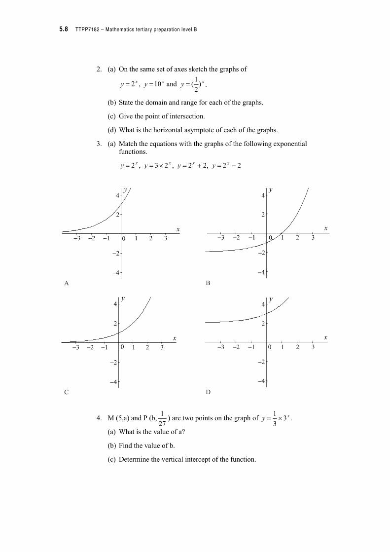
3. (a) Match the equations with the graphs of the following exponential functions.
4. M (5,a) and P (b, ) are two points on the graph of .
(a) What is the value of a?
(b) Find the value of b.
(c) Determine the vertical intercept of the function.
xxx yyy )2
1( and 10 ,2 !!!
22 ,22 ,23 ,2 "!#! !!xxxx yyyy
xx
y
−3 −2 −1 0 1 2 3
−2
−4
2
4
y
−3 −2 −1 0 1 2 3
−2
−4
2
4
x
−3 −2 −1 0 1 2 3
−4
−2
2
4
y
−4
x
y
−3 −2 −1 0 1 2 3
−2
2
4
A B
C D
27
1 xy 33
1 !
Module B5 – Exponential and logarithmic functions 5.9
5.1.2 The exponential function
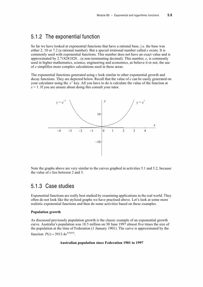
So far we have looked at exponential functions that have a rational base, i.e. the base was either 2, 10 or 7.2 (a rational number). But a special irrational number called e exists. It is commonly used with exponential functions. This number does not have an exact value and is approximated by 2.718281828…(a non-terminating decimal). This number, e, is commonly used in higher mathematics, science, engineering and economics, as believe it or not, the use of e simplifies more complex calculations used in these areas.
The exponential functions generated using e look similar to other exponential growth and decay functions. They are depicted below. Recall that the value of e can be easily generated on your calculator using the key. All you have to do is calculate the value of the function at x = 1. If you are unsure about doing this consult your tutor.
Note the graphs above are very similar to the curves graphed in activities 5.1 and 5.2, because the value of e lies between 2 and 3.
5.1.3 Case studies
Exponential functions are really best studied by examining applications in the real world. They often do not look like the stylized graphs we have practised above. Let’s look at some more realistic exponential functions and then do some activities based on these examples.
Population growth
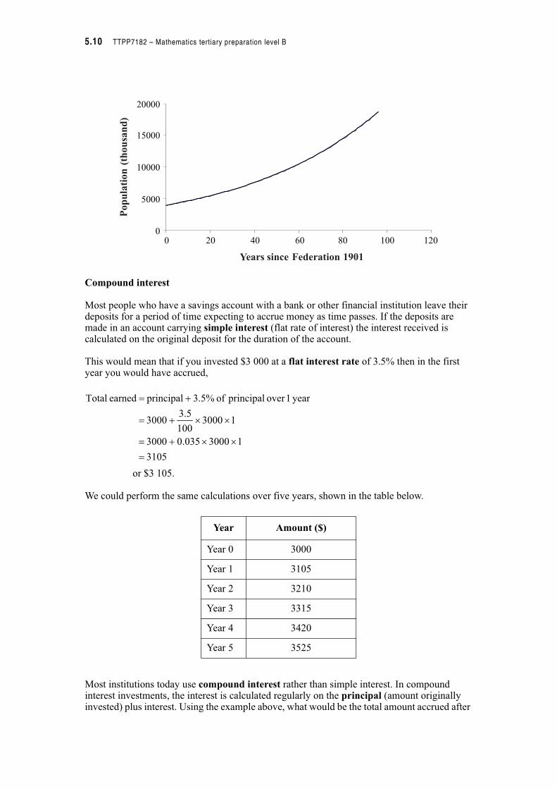
As discussed previously population growth is the classic example of an exponential growth curve. Australia’s population was 18.5 million on 30 June 1997 almost five times the size of the population at the time of Federation (1 January 1901). The curve is approximated by the
function .
Australian population since Federation 1901 to 1997
xe
x
y
−4 −3 −2 −1 0 1 2 3 4
−10
10
y e=−x
y e=x
tetP 0163.04.3913)( !
5.10 TTPP7182 – Mathematics tertiary preparation level B
Compound interest
Most people who have a savings account with a bank or other financial institution leave their deposits for a period of time expecting to accrue money as time passes. If the deposits are made in an account carrying simple interest (flat rate of interest) the interest received is calculated on the original deposit for the duration of the account.
This would mean that if you invested $3 000 at a flat interest rate of 3.5% then in the first year you would have accrued,
or $3 105.
We could perform the same calculations over five years, shown in the table below.
Most institutions today use compound interest rather than simple interest. In compound interest investments, the interest is calculated regularly on the principal (amount originally invested) plus interest. Using the example above, what would be the total amount accrued after
Year Amount ($)
Year 0 3000
Year 1 3105
Year 2 3210
Year 3 3315
Year 4 3420
Year 5 3525
00 20 40 60 80 100 120
5000
10000
15000
20000
Popula
tion
(thousa
nd)
Years since Federation 1901
3105
13000035.03000
13000100
5.33000
year 1over principal of 3.5%principalearned Total
!
#!
#!
#!
Module B5 – Exponential and logarithmic functions 5.11
the first year? So after year one we would have the original principal plus 3.5% of that principal. In fact this means that we would have 103.5% of the principal. We can work this out mathematically as follows.
or $3 105
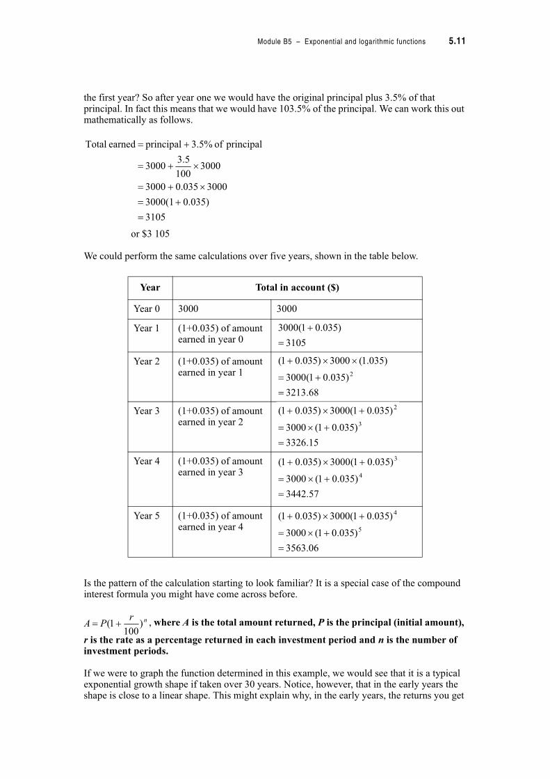
We could perform the same calculations over five years, shown in the table below.
Is the pattern of the calculation starting to look familiar? It is a special case of the compound interest formula you might have come across before.
, where A is the total amount returned, P is the principal (initial amount),
r is the rate as a percentage returned in each investment period and n is the number of investment periods.
If we were to graph the function determined in this example, we would see that it is a typical exponential growth shape if taken over 30 years. Notice, however, that in the early years the shape is close to a linear shape. This might explain why, in the early years, the returns you get
Year Total in account ($)
Year 0 3000 3000
Year 1 (1+0.035) of amount earned in year 0
Year 2 (1+0.035) of amount earned in year 1
Year 3 (1+0.035) of amount earned in year 2
Year 4 (1+0.035) of amount earned in year 3
Year 5 (1+0.035) of amount earned in year 4
3105
0.035)3000(1
30000.0353000
3000100
5.33000
principal of 3.5%principalearned Total
!
#!
#!
#!
#!
3105
)035.01(3000
!
#
68.3213
)035.01(3000
)035.1(3000)035.01(
2
!
#!
#
15.3326
)035.01(3000
)035.01(3000)035.01(
3
2
!
# !
# #
57.3442
)035.01(3000
)035.01(3000)035.01(
4
3
!
# !
# #
06.3563
)035.01(3000
)035.01(3000)035.01(
5
4
!
# !
# #
nrPA )
1001( #!

5.12 TTPP7182 – Mathematics tertiary preparation level B
from compound interest are only marginally better than the returns you get from simple interest. Look back at the two tables and see what the values were.
Total amount accrued applying compound interest
2500.000 5 10 15 20 25 30
3500.00
4500.00
5500.00
6500.00
7500.00Tota
lam
ount($
)
Years of investment
A = 3000 (1 + 0.035)n
A bit of history… For interest only
The importance of e was first recognised by the Swiss mathematician Leonhard Euler. He gave it its name, derived many relationships using it and developed several different ways to calculate it. You might like to think about this way of looking at the derivation of e.
If we invested $1 at 100% compound interest each year then the returns (A) on our
investment would be represented by the formula , since P = 1,
r = 100/number of periods
If interest is paid yearly you receive
If interest is paid monthly you receive (12 is months per year)
If interest is paid daily you receive (365 is days per year)
If interest is paid hourly you receive (8760 is hours per year)
So it appears that we can get very close to the value of e if we find the value of as n gets very large. Do not learn this.
n
n
rPA )
11()
1001( #!#!
2)1
11()
11( 1
!#!#!n
nA
61.2)12
11()
11( 12
!#!#!n
nA
71.2)365
11()
11( 365
!#!#!n
nA
7181235.2)8760
11()
11( 8760
!#!#!n
nA
n
nA )
11( #!
Module B5 – Exponential and logarithmic functions 5.13
Depreciation
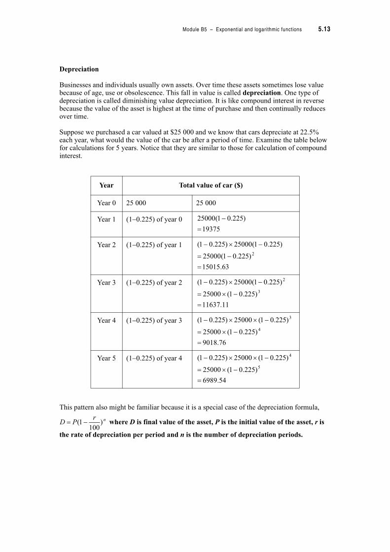
Businesses and individuals usually own assets. Over time these assets sometimes lose value because of age, use or obsolescence. This fall in value is called depreciation. One type of depreciation is called diminishing value depreciation. It is like compound interest in reverse because the value of the asset is highest at the time of purchase and then continually reduces over time.
Suppose we purchased a car valued at $25 000 and we know that cars depreciate at 22.5% each year, what would the value of the car be after a period of time. Examine the table below for calculations for 5 years. Notice that they are similar to those for calculation of compound interest.
This pattern also might be familiar because it is a special case of the depreciation formula,
where D is final value of the asset, P is the initial value of the asset, r is
the rate of depreciation per period and n is the number of depreciation periods.
Year Total value of car ($)
Year 0 25 000 25 000
Year 1 (1"0.225) of year 0
Year 2 (1"0.225) of year 1
Year 3 (1"0.225) of year 2
Year 4 (1"0.225) of year 3
Year 5 (1"0.225) of year 4
19375
)225.01(25000
!
"
63.15015
)225.01(25000
)225.01(25000)225.01(
2
!
"!
" "
11.11637
)225.01(25000
)225.01(25000)225.01(
3
2
!
" !
" "
76.9018
)225.01(25000
)225.01(25000)225.01(
4
3
!
" !
" "
54.6989
)225.01(25000
)225.01(25000)225.01(
5
4
!
" !
" "
nrPD )
1001( "!

5.14 TTPP7182 – Mathematics tertiary preparation level B
If we were to graph the function determined in the example above we would see that it is a typical exponential decay shape if taken over 20 years.
Depreciation of a car
Chemical reactions
Some chemicals when in solution break down into different components so that the concentration of the original compound changes over time. In 1864 Guildberg and Waage recognized that at a constant temperature the rate of this type of reaction followed an exponential decay curve. An example of this is the breakdown of di-nitrogen pentoxide into nitrogen oxide and oxygen. When this decomposition is graphed we get the following figure.
Composition of di-nitrogen pentoxide
The equation for this function is:
, where t is in hours and C(t) is concentration in moles per litre. The initial
amount of chemical in the solution was 0.87 moles per litre.
The above show some specific applications of exponential functions. Let’s look as some examples using these types of applications.
0
5000
10000
15000
20000
25000
30000
0 5 10 15 20 25
Valu
eofca
r($
)
Number of years
0.00
0.20
0.40
0.60
0.80
1.00
0 1 2 3 4 5 6Conce
ntr
ation
(mole
sper
litr
e)
Time (hours)
p g
tetC 30.087.0)( "!
Module B5 – Exponential and logarithmic functions 5.15
Example
Peter invested $8 000 in a fixed term deposit for 3 years attracting 12% pa interest compounded quarterly. What would be his total return?
We can use the formula to calculate the amount returned but first we need to
determine the components of the formula. P, the principal is the amount invested and is $8 000. n is the number of interest gathering periods, so because the interest is accrued quarterly for 3 years then n must be 12. r is the interest rate as a percentage at each accruing period. Since the interest is defined as 12% pa (per annum) it should be divided by 4 to get the interest rate at each quarter. Therefore r is 3%.
So the amount A is given by, , , substituting into the
formula,
The amount returned is $11 406.09.
Example
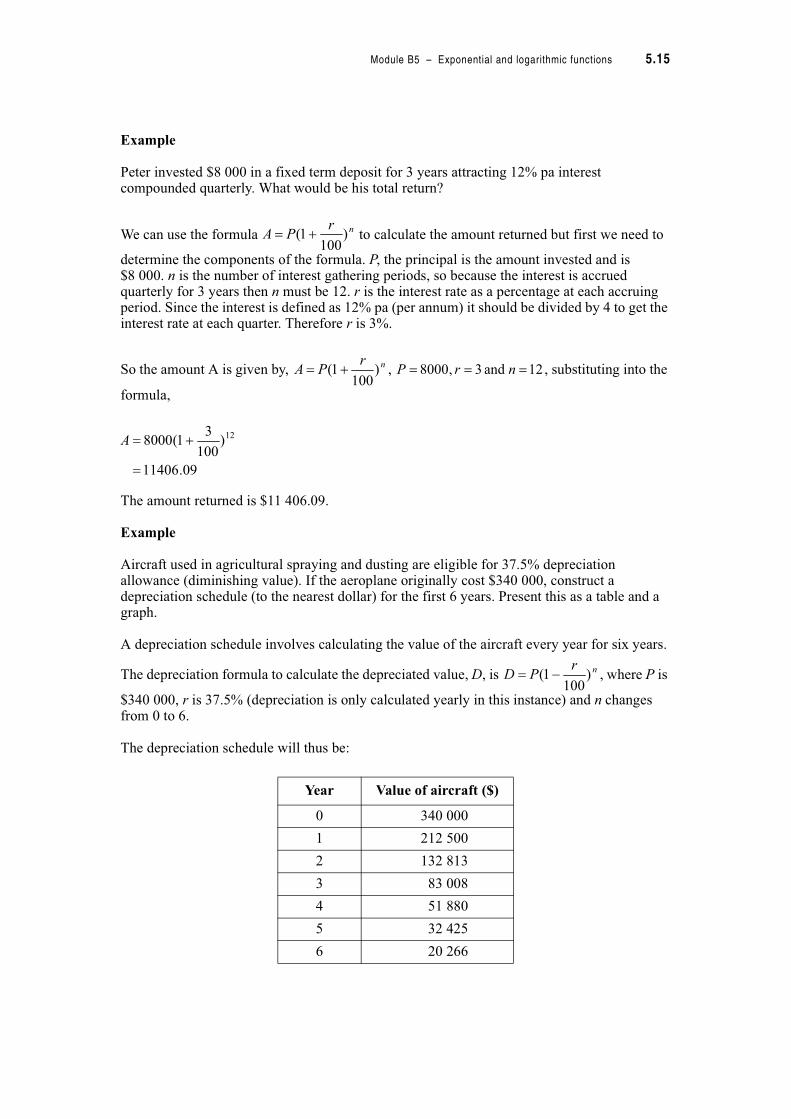
Aircraft used in agricultural spraying and dusting are eligible for 37.5% depreciation allowance (diminishing value). If the aeroplane originally cost $340 000, construct a depreciation schedule (to the nearest dollar) for the first 6 years. Present this as a table and a graph.
A depreciation schedule involves calculating the value of the aircraft every year for six years.
The depreciation formula to calculate the depreciated value, D, is , where P is
$340 000, r is 37.5% (depreciation is only calculated yearly in this instance) and n changes from 0 to 6.
The depreciation schedule will thus be:
Year Value of aircraft ($)
0 340 000
1 212 500
2 132 813
3 83 008
4 51 880
5 32 425
6 20 266
nrPA )
1001( #!
nrPA )
1001( #! 12 and 3,8000 !!! nrP
09.11406
)100
31(8000 12
!
#!A
nrPD )
1001( "!
5.16 TTPP7182 – Mathematics tertiary preparation level B
Depreciation of aircraft over 6 years
Example
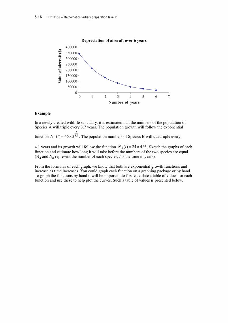
In a newly created wildlife sanctuary, it is estimated that the numbers of the population of Species A will triple every 3.7 years. The population growth will follow the exponential
function . The population numbers of Species B will quadruple every
4.1 years and its growth will follow the function . Sketch the graphs of each
function and estimate how long it will take before the numbers of the two species are equal. (NA and NB represent the number of each species, t is the time in years).
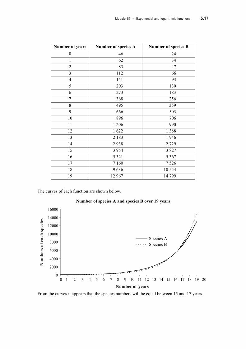
From the formulas of each graph, we know that both are exponential growth functions and increase as time increases. You could graph each function on a graphing package or by hand. To graph the functions by hand it will be important to first calculate a table of values for each function and use these to help plot the curves. Such a table of values is presented below.
0
50000
100000
250000
150000
300000
200000
350000
400000
0 1 2 3 654 7
Valu
eofair
craft
($)
Number of years
7.3346)(
t
A tN !
1.4424)(
t
B tN !
Module B5 – Exponential and logarithmic functions 5.17
The curves of each function are shown below.
Number of species A and species B over 19 years
From the curves it appears that the species numbers will be equal between 15 and 17 years.
Number of years Number of species A Number of species B
0 46 24
1 62 34
2 83 47
3 112 66
4 151 93
5 203 130
6 273 183
7 368 256
8 495 359
9 666 503
10 896 706
11 1 206 990
12 1 622 1 388
13 2 183 1 946
14 2 938 2 729
15 3 954 3 827
16 5 321 5 367
17 7 160 7 526
18 9 636 10 554
19 12 967 14 799
00 321 4 5 6 7 8 9 10 11 12 13 14 15 16 17 18 19 20
Species A
Species B
2000
4000
6000
8000
10000
12000
14000
16000
Number of years
Num
ber
sofea
chsp
ecie
s
5.18 TTPP7182 – Mathematics tertiary preparation level B
Example
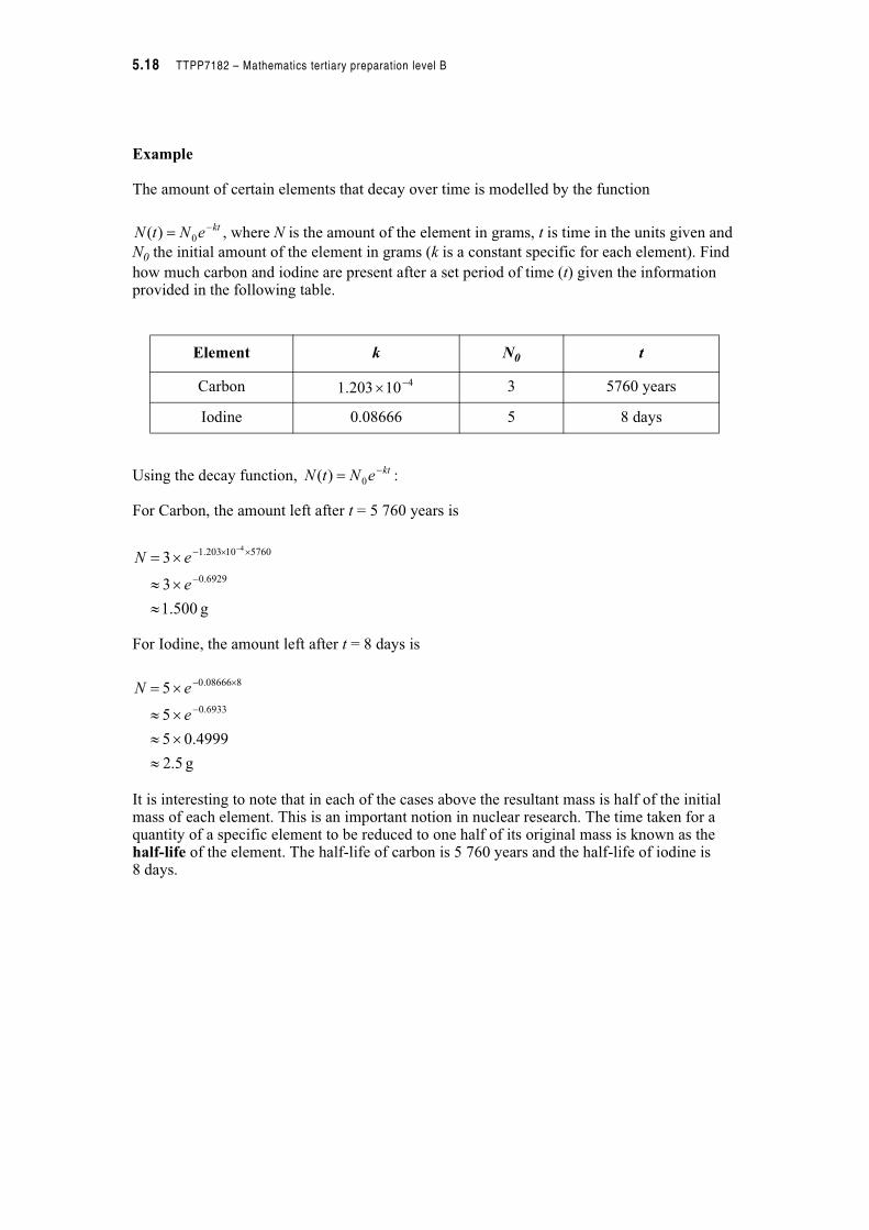
The amount of certain elements that decay over time is modelled by the function
, where N is the amount of the element in grams, t is time in the units given and
N0 the initial amount of the element in grams (k is a constant specific for each element). Find
how much carbon and iodine are present after a set period of time (t) given the information provided in the following table.
Using the decay function, :
For Carbon, the amount left after t = 5 760 years is
For Iodine, the amount left after t = 8 days is
It is interesting to note that in each of the cases above the resultant mass is half of the initial mass of each element. This is an important notion in nuclear research. The time taken for a quantity of a specific element to be reduced to one half of its original mass is known as the half-life of the element. The half-life of carbon is 5 760 years and the half-life of iodine is 8 days.
Element k N0 t
Carbon 3 5760 years
Iodine 5 8 days
kteNtN "! 0)(
410203.1 "
08666.0
kteNtN "! 0)(
g 500.1
3
3
6929.0
576010203.1 4
$
$
!
"
""
e
eN
g 5.2
4999.05
5
5
6933.0
808666.0
$
$
$
!
"
"
e
eN
Module B5 – Exponential and logarithmic functions 5.19
Activity 5.4
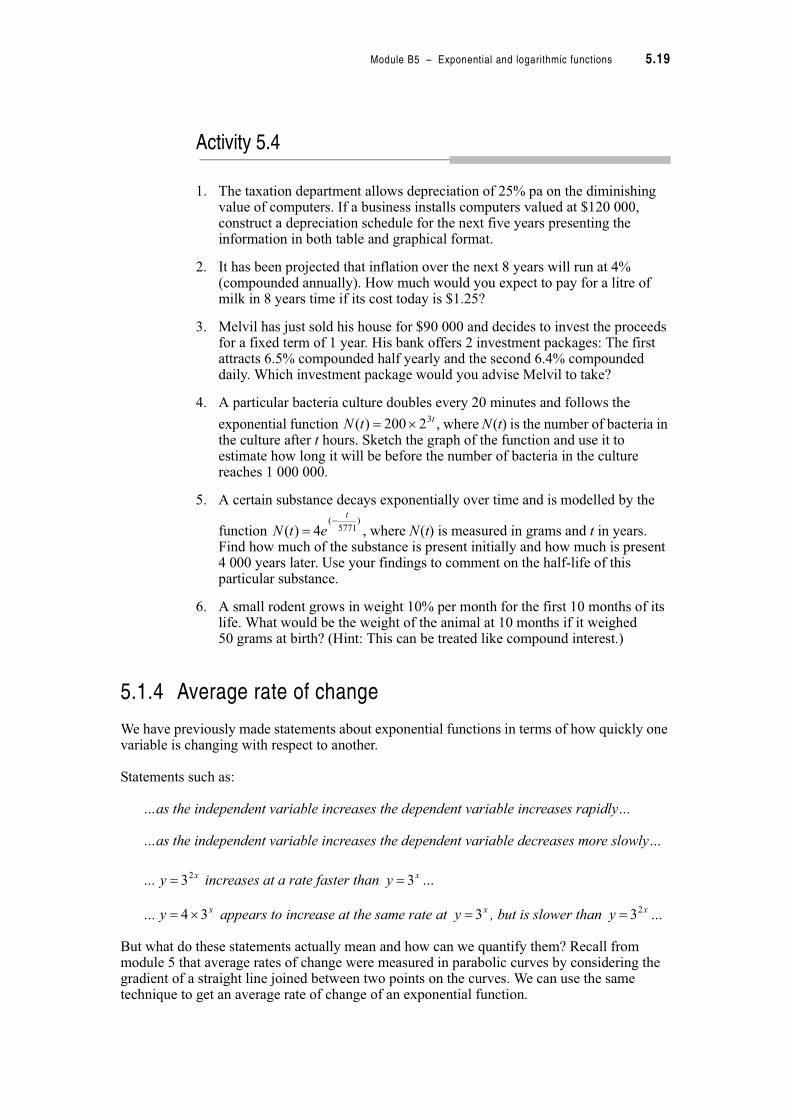
1. The taxation department allows depreciation of 25% pa on the diminishing value of computers. If a business installs computers valued at $120 000, construct a depreciation schedule for the next five years presenting the information in both table and graphical format.
2. It has been projected that inflation over the next 8 years will run at 4% (compounded annually). How much would you expect to pay for a litre of milk in 8 years time if its cost today is $1.25?
3. Melvil has just sold his house for $90 000 and decides to invest the proceeds for a fixed term of 1 year. His bank offers 2 investment packages: The first attracts 6.5% compounded half yearly and the second 6.4% compounded daily. Which investment package would you advise Melvil to take?
4. A particular bacteria culture doubles every 20 minutes and follows the
exponential function , where N(t) is the number of bacteria in the culture after t hours. Sketch the graph of the function and use it to estimate how long it will be before the number of bacteria in the culture reaches 1 000 000.
5. A certain substance decays exponentially over time and is modelled by the
function , where N(t) is measured in grams and t in years. Find how much of the substance is present initially and how much is present 4 000 years later. Use your findings to comment on the half-life of this particular substance.
6. A small rodent grows in weight 10% per month for the first 10 months of its life. What would be the weight of the animal at 10 months if it weighed 50 grams at birth? (Hint: This can be treated like compound interest.)
5.1.4 Average rate of change
We have previously made statements about exponential functions in terms of how quickly one variable is changing with respect to another.
Statements such as:
…as the independent variable increases the dependent variable increases rapidly…
…as the independent variable increases the dependent variable decreases more slowly…
… increases at a rate faster than …
… appears to increase at the same rate at , but is slower than …
But what do these statements actually mean and how can we quantify them? Recall from module 5 that average rates of change were measured in parabolic curves by considering the gradient of a straight line joined between two points on the curves. We can use the same technique to get an average rate of change of an exponential function.
ttN 32200)( !
)5771
(
4)(
t
etN"
!
xy 23! xy 3!
xy 34 !xy 3! xy 23!
5.20 TTPP7182 – Mathematics tertiary preparation level B
Let’s consider an example for exponential growth and one example for exponential decay.
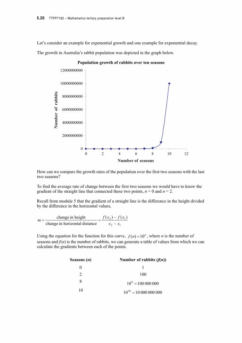
The growth in Australia’s rabbit population was depicted in the graph below.
Population growth of rabbits over ten seasons
How can we compare the growth rates of the population over the first two seasons with the last two seasons?
To find the average rate of change between the first two seasons we would have to know the gradient of the straight line that connected these two points, n = 0 and n = 2.
Recall from module 5 that the gradient of a straight line is the difference in the height divided by the difference in the horizontal values,
Using the equation for the function for this curve, , where n is the number of
seasons and f(n) is the number of rabbits, we can generate a table of values from which we can calculate the gradients between each of the points.
Seasons (n) Number of rabbits (f(n))
0 1
2 100
8
10
0
0 2 4 6 8 10 12
2000000000
4000000000
6000000000
8000000000
10000000000
12000000000
Num
ber
of
rabbits
Number of seasons
12
12 )()(
distance horizontalin change
heightin change
xx
xfxfm
"
"!!
nnf 10)( !
000 000 100108!
000 000 000 101010!
Module B5 – Exponential and logarithmic functions 5.21
Average rate of change over the first two seasons is
Average rate of change over the last two seasons is
In real terms, because the gradients are both positive, the function is increasing and population is growing at a rate of 50 rabbits per season over the first two seasons compared with 4 950 000 000 rabbits per season over the last two seasons. This means that population growth rate was small at the start but increased very rapidly over the last two seasons, and is thus increasing.
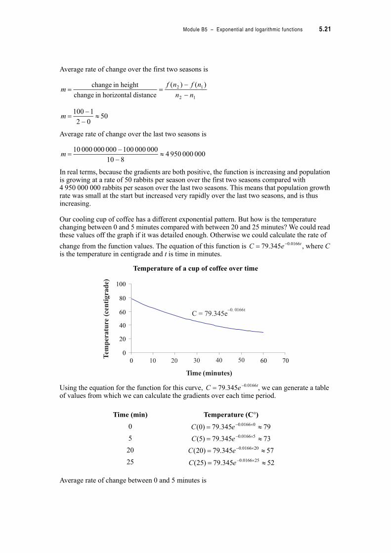
Our cooling cup of coffee has a different exponential pattern. But how is the temperature changing between 0 and 5 minutes compared with between 20 and 25 minutes? We could read these values off the graph if it was detailed enough. Otherwise we could calculate the rate of
change from the function values. The equation of this function is , where C is the temperature in centigrade and t is time in minutes.
Temperature of a cup of coffee over time
Using the equation for the function for this curve, , we can generate a table of values from which we can calculate the gradients over each time period.
Average rate of change between 0 and 5 minutes is
Time (min) Temperature (C#)
0
5
20
25
12
12 )()(
distance horizontalin change
heightin change
nn
nfnfm
"
"!!
5002
1100$
"
"!m
000 000 950 4810
000 000 100000 000 000 10$
"
"!m
teC 0166.0345.79 "!
20
40
60
80
0
0 60 70
20
40
60
80
100
Tem
per
atu
re(c
entigra
de)
Time (minutes)
10 20 30 40 50
C = 79.345e−0. 0166t
teC 0166.0345.79 "!
79345.79)0( 00166.0$!
"eC
73345.79)5( 50166.0$!
"eC
57345.79)20( 200166.0$!
"eC
52345.79)25( 250166.0$!
"eC
5.22 TTPP7182 – Mathematics tertiary preparation level B
Average rate of change between 20 and 25 minutes is
In real terms, because the gradients are both negative, the function is decreasing. The temperature is dropping at an average rate of 1.2 degrees per minute during the first five minutes and 1 degree per minute between 20 and 25 minutes. This means that the cooling rate is decreasing or getting slower i.e. the coffee is cooling more slowly as time passes.
Activity 5.5
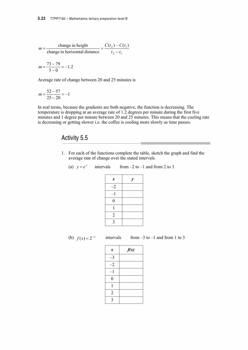
1. For each of the functions complete the table, sketch the graph and find the average rate of change over the stated intervals.
(a) intervals from –2 to –1 and from 2 to 3
(b) intervals from –3 to –1 and from 1 to 3
x y
–2
–1
0
1
2
3
x f(x)
–3
–2
–1
0
1
2
3
12
12 )()(
distance horizontalin change
heightin change
tt
tCtCm
"
"!!
2.105
7973"!
"
"!m
12025
5752"!
"
"!m
xey !
xxf "! 2)(
Module B5 – Exponential and logarithmic functions 5.23
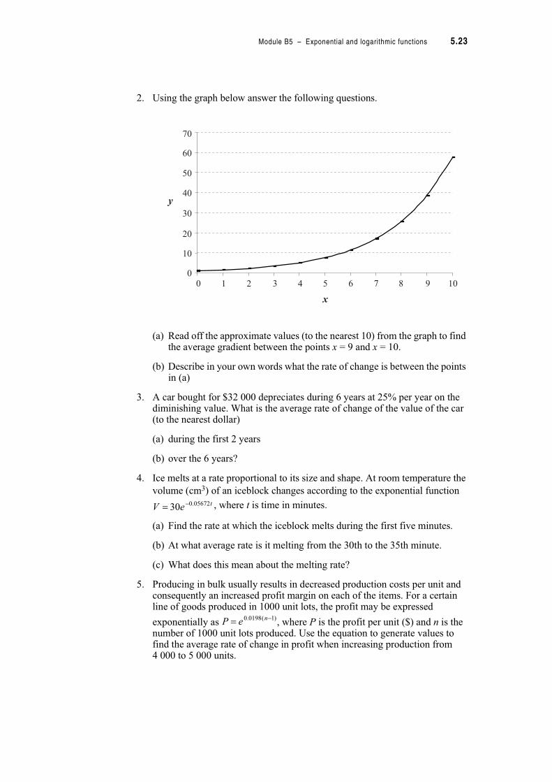
2. Using the graph below answer the following questions.
(a) Read off the approximate values (to the nearest 10) from the graph to find the average gradient between the points x = 9 and x = 10.
(b) Describe in your own words what the rate of change is between the points in (a)
3. A car bought for $32 000 depreciates during 6 years at 25% per year on the diminishing value. What is the average rate of change of the value of the car (to the nearest dollar)
(a) during the first 2 years
(b) over the 6 years?
4. Ice melts at a rate proportional to its size and shape. At room temperature the
volume (cm3) of an iceblock changes according to the exponential function
, where t is time in minutes.
(a) Find the rate at which the iceblock melts during the first five minutes.
(b) At what average rate is it melting from the 30th to the 35th minute.
(c) What does this mean about the melting rate?
5. Producing in bulk usually results in decreased production costs per unit and consequently an increased profit margin on each of the items. For a certain line of goods produced in 1000 unit lots, the profit may be expressed
exponentially as , where P is the profit per unit ($) and n is the number of 1000 unit lots produced. Use the equation to generate values to find the average rate of change in profit when increasing production from 4 000 to 5 000 units.
x
y
0
0
10
20
30
40
50
60
70
31 2 6 7 854 9 10
teV 05672.030 "!
)1(0198.0 "!
neP
5.24 TTPP7182 – Mathematics tertiary preparation level B
5.1.5 The inverse of the exponential function
In previous sections of this module we set up a function from which we could calculate the number of rabbits after a given number of seasons. This function was where f(n) is the number of rabbits and n is the number of seasons. Writing the function in this way shows that we are thinking of the number of rabbits as a function of seasons.
Now suppose that instead of wanting to calculate the number of rabbits for any season, we were given the number of rabbits and wanted to know how many seasons it had taken to reach this number…a very reasonable question for an ecologist to ask. How could we do this?
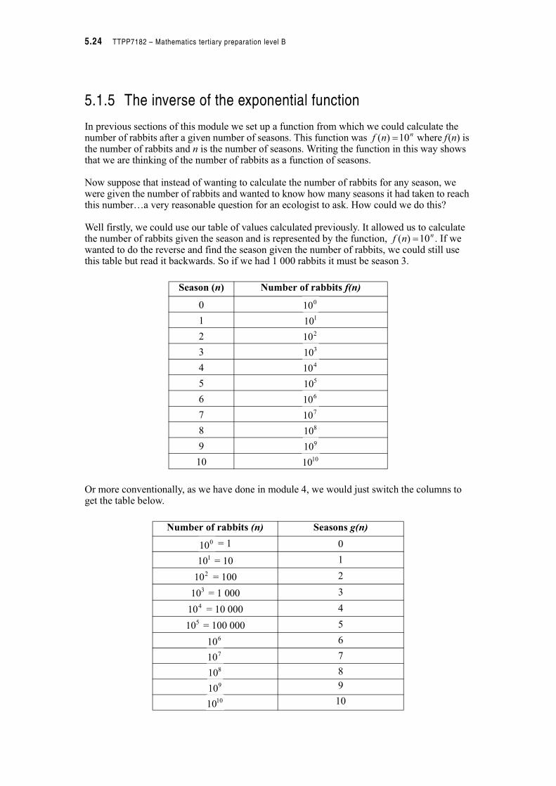
Well firstly, we could use our table of values calculated previously. It allowed us to calculate the number of rabbits given the season and is represented by the function, . If we wanted to do the reverse and find the season given the number of rabbits, we could still use this table but read it backwards. So if we had 1 000 rabbits it must be season 3.
Or more conventionally, as we have done in module 4, we would just switch the columns to get the table below.
Season (n) Number of rabbits f(n)
0
1
2
3
4
5
6
7
8
9
10
Number of rabbits (n) Seasons g(n)
= 1 0
= 10 1
= 100 2
= 1 000 3
= 10 000 4
= 100 000 5
6
7
8
9
10
nnf 10)( !
nnf 10)( !
010110210310410510610710810910
1010
010110
210310
410510
610710810910
1010
Module B5 – Exponential and logarithmic functions 5.25
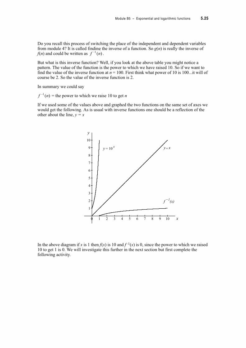
Do you recall this process of switching the place of the independent and dependent variables from module 4? It is called finding the inverse of a function. So g(n) is really the inverse of f(n) and could be written as .
But what is this inverse function? Well, if you look at the above table you might notice a pattern. The value of the function is the power to which we have raised 10. So if we want to find the value of the inverse function at n = 100. First think what power of 10 is 100...it will of course be 2. So the value of the inverse function is 2.
In summary we could say
= the power to which we raise 10 to get n
If we used some of the values above and graphed the two functions on the same set of axes we would get the following. As is usual with inverse functions one should be a reflection of the other about the line, y = x
In the above diagram if x is 1 then f(x) is 10 and f–1(x) is 0, since the power to which we raised 10 to get 1 is 0. We will investigate this further in the next section but first complete the following activity.
)(1 nf "
)(1 nf "
0 1 2 3 4 5 6 7 8 9 10
1
2
3
4
5
6
7
8
9
10
x
y
yx
= 10 y x =
f−1
(x)
5.26 TTPP7182 – Mathematics tertiary preparation level B
Activity 5.6
1. In the compound interest example in section 5.1.3 we looked at an investment of $3 000 at 3.5% compounded annually and found that it had amounted to $3 563 in 5 years.
(a) Set up a table showing number of years (n) and amount earned A(n).
(b) Use this table to produce the inverse of this function.
(c) Describe the use of the inverse function.
(d) Determine approximately how long it will take for $3 000 to grow to $4 000.
2. By the year 2000 Australia’s population in expected to be 19.5 million and
after that growing exponentially as , where P is millions of
people and t is years.
(a) Set up a table of value for this function.
(b) Use this table to set up a table of values for the inverse of the P function.
(c) Use this table to find when the population will reach 22.5 million.
3. (a) On the same set of axes draw
••
(b) Use the two graph above to roughly sketch the inverse of
4. The decay of radium is modelled by the function , where R is
the amount remaining (g), t is time (weeks) and R0 is the original amount.
Generate a table of values to find the half-life of 10 g of radium. Remember that half-life means time to reach half of the original amount.
5. Carbon dating involves the measurement of concentration of carbon
remaining in an object. The decay function is used to determine the age of a bone taken from an archaeological dig, where C is the concentration remaining and t is time in thousands of years. It is found that 60% of the original carbon remains in the samples. Estimate the age of the bone. (Hint: Develop a table of values for the inverse function and find when C = 60).
tetP 0163.05.19)( !
100 , %%! xxy
xy 1.010!
xy 1.010!
teRR 077.00
"!
tC 1786.02100 " !
Module B5 – Exponential and logarithmic functions 5.27
5.2 Logarithmic functions
5.2.1 What is a logarithm?
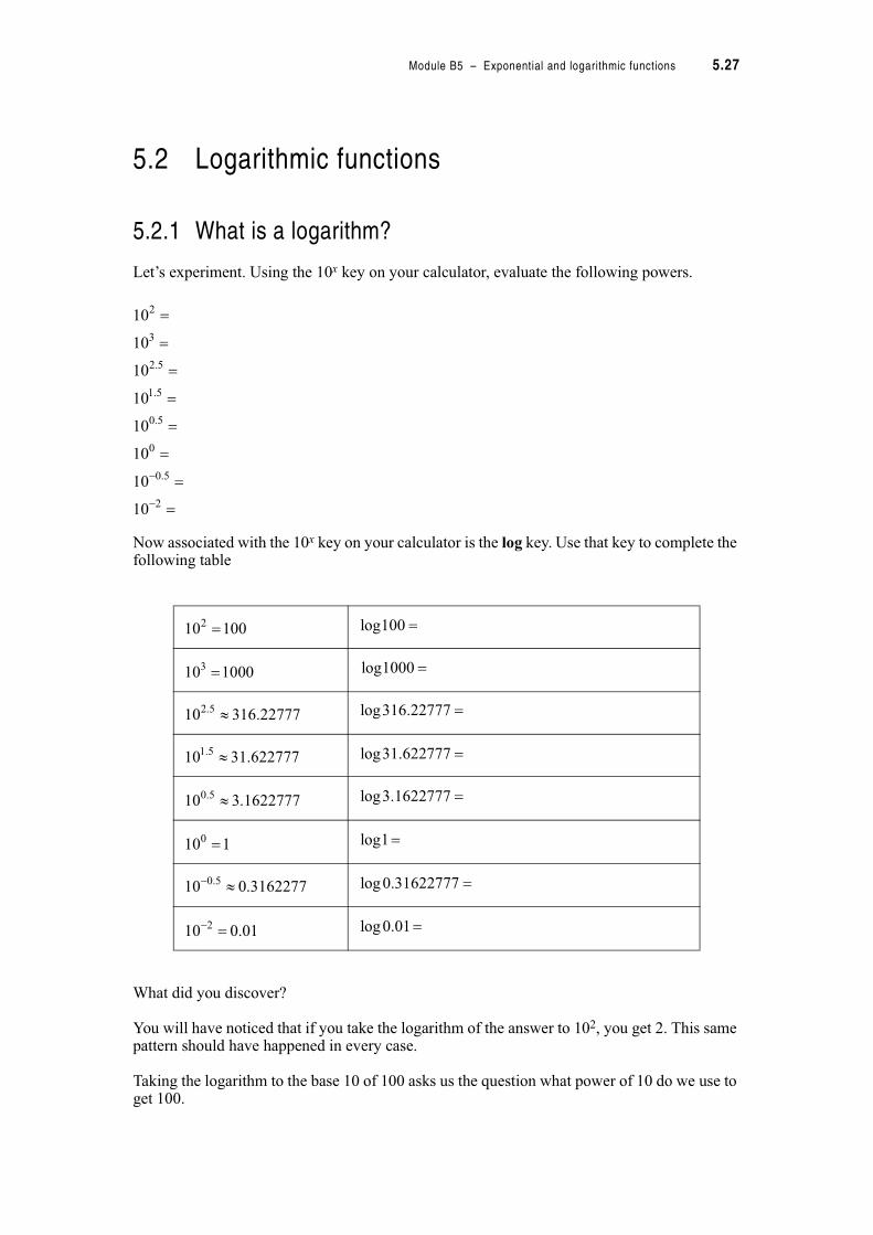
Let’s experiment. Using the 10x key on your calculator, evaluate the following powers.
Now associated with the 10x key on your calculator is the log key. Use that key to complete the following table
What did you discover?
You will have noticed that if you take the logarithm of the answer to 102, you get 2. This same pattern should have happened in every case.
Taking the logarithm to the base 10 of 100 asks us the question what power of 10 do we use to get 100.
2
3
2.5
1.5
0.5
0
0.5
2
10
10
10
10
10
10
10
10
"
"
!
!
!
!
!
!
!
!
210 100! log100 !
310 1000! log1000 !
2.510 316.22777$ log316.22777 !
1.510 31.622777$ log31.622777 !
0.510 3.1622777$ log3.1622777 !
010 1! log1!
0.510 0.3162277"$ log0.31622777 !
210 0.01"! log0.01!
5.28 TTPP7182 – Mathematics tertiary preparation level B
The logarithmic function is actually the inverse of the exponential function.
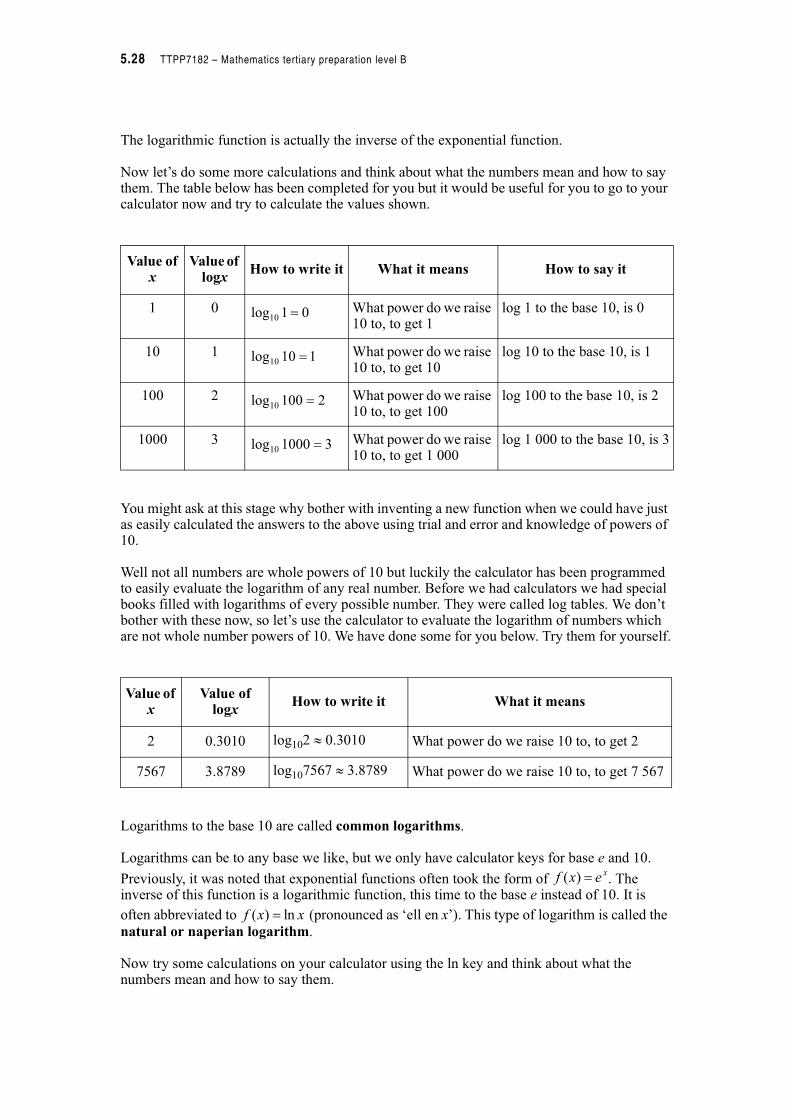
Now let’s do some more calculations and think about what the numbers mean and how to say them. The table below has been completed for you but it would be useful for you to go to your calculator now and try to calculate the values shown.
You might ask at this stage why bother with inventing a new function when we could have just as easily calculated the answers to the above using trial and error and knowledge of powers of 10.
Well not all numbers are whole powers of 10 but luckily the calculator has been programmed to easily evaluate the logarithm of any real number. Before we had calculators we had special books filled with logarithms of every possible number. They were called log tables. We don’t bother with these now, so let’s use the calculator to evaluate the logarithm of numbers which are not whole number powers of 10. We have done some for you below. Try them for yourself.
Logarithms to the base 10 are called common logarithms.
Logarithms can be to any base we like, but we only have calculator keys for base e and 10.
Previously, it was noted that exponential functions often took the form of . The inverse of this function is a logarithmic function, this time to the base e instead of 10. It is
often abbreviated to (pronounced as ‘ell en x’). This type of logarithm is called the natural or naperian logarithm.
Now try some calculations on your calculator using the ln key and think about what the numbers mean and how to say them.
Value of x
Value of logx
How to write it What it means How to say it
1 0 What power do we raise 10 to, to get 1
log 1 to the base 10, is 0
10 1 What power do we raise 10 to, to get 10
log 10 to the base 10, is 1
100 2 What power do we raise 10 to, to get 100
log 100 to the base 10, is 2
1000 3 What power do we raise 10 to, to get 1 000
log 1 000 to the base 10, is 3
Value of x
Value of logx
How to write it What it means
2 0.3010 log102 $ 0.3010 What power do we raise 10 to, to get 2
7567 3.8789 log107567 $ 3.8789 What power do we raise 10 to, to get 7 567
01log10 !
110log10 !
2100log10 !
31000log10 !
xexf !)(
( ) lnf x x!
Module B5 – Exponential and logarithmic functions 5.29
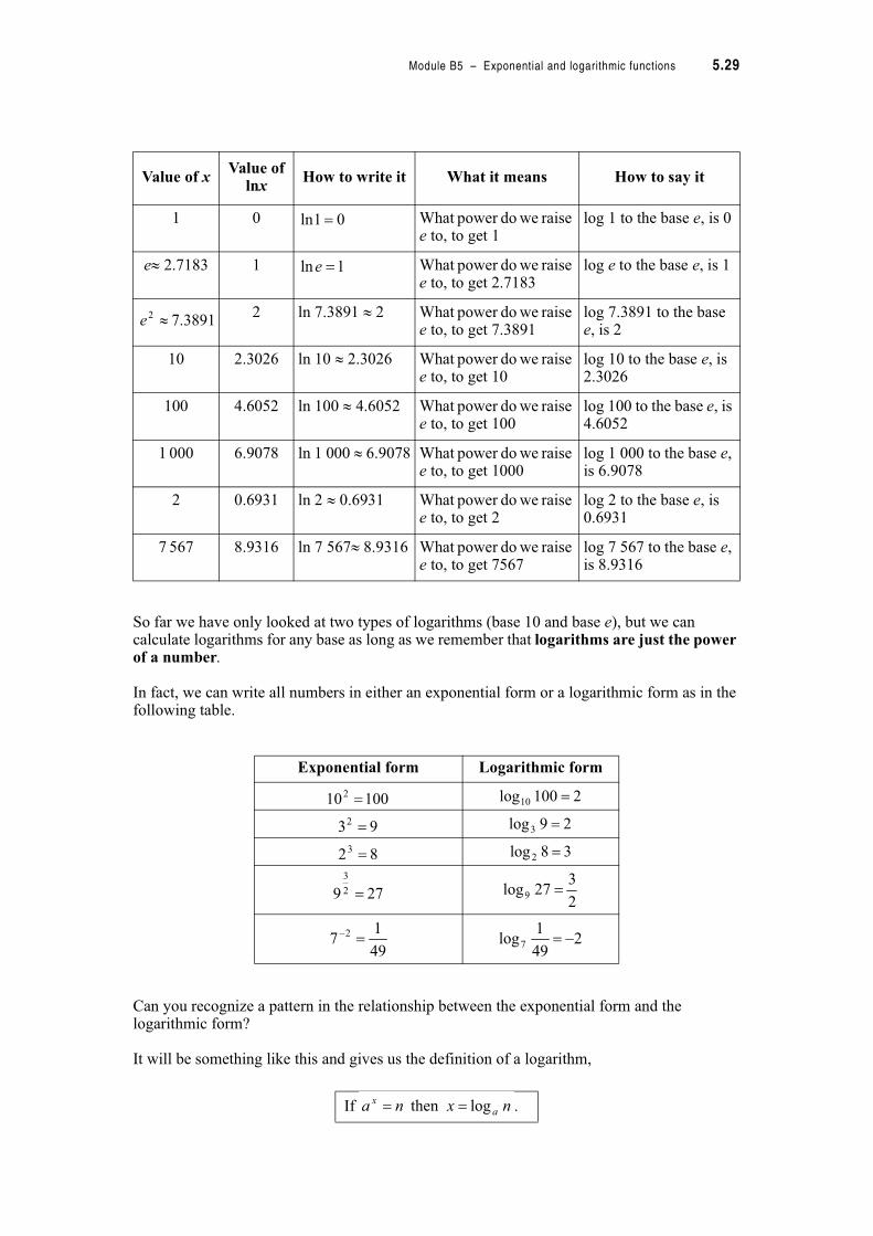
So far we have only looked at two types of logarithms (base 10 and base e), but we can calculate logarithms for any base as long as we remember that logarithms are just the power of a number.
In fact, we can write all numbers in either an exponential form or a logarithmic form as in the following table.
Can you recognize a pattern in the relationship between the exponential form and the logarithmic form?
It will be something like this and gives us the definition of a logarithm,
Value of xValue of
lnxHow to write it What it means How to say it
1 0 What power do we raise e to, to get 1
log 1 to the base e, is 0
e$ 2.7183 1 What power do we raise e to, to get 2.7183
log e to the base e, is 1
2 ln 7.3891 $ 2 What power do we raise e to, to get 7.3891
log 7.3891 to the base e, is 2
10 2.3026 ln 10 $ 2.3026 What power do we raise e to, to get 10
log 10 to the base e, is 2.3026
100 4.6052 ln 100 $ 4.6052 What power do we raise e to, to get 100
log 100 to the base e, is 4.6052
1 000 6.9078 ln 1 000 $ 6.9078 What power do we raise e to, to get 1000
log 1 000 to the base e, is 6.9078
2 0.6931 ln 2 $ 0.6931 What power do we raise e to, to get 2
log 2 to the base e, is 0.6931
7 567 8.9316 ln 7 567$ 8.9316 What power do we raise e to, to get 7567
log 7 567 to the base e, is 8.9316
Exponential form Logarithmic form
If .
01ln !
1ln !e
3891.72$e
100102! 2100log10 !
932! 29log3 !
823! 38log2 !
279 2
3
!2
327log9 !
49
17 2
!" 2
49
1log7 "!
log then nxna ax
!!
5.30 TTPP7182 – Mathematics tertiary preparation level B
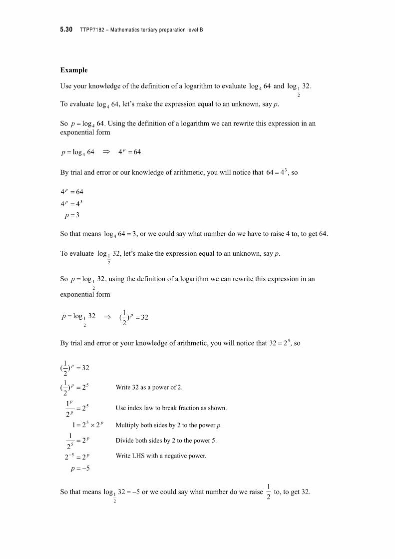
Example
Use your knowledge of the definition of a logarithm to evaluate and .
To evaluate , let’s make the expression equal to an unknown, say p.
So . Using the definition of a logarithm we can rewrite this expression in an
exponential form
&
By trial and error or our knowledge of arithmetic, you will notice that , so
So that means , or we could say what number do we have to raise 4 to, to get 64.
To evaluate , let’s make the expression equal to an unknown, say p.
So , using the definition of a logarithm we can rewrite this expression in an
exponential form
&
By trial and error or your knowledge of arithmetic, you will notice that , so
So that means or we could say what number do we raise to, to get 32.
Write 32 as a power of 2.
Use index law to break fraction as shown.
Multiply both sides by 2 to the power p.
Divide both sides by 2 to the power 5.
Write LHS with a negative power.
64log 4 32log
2
1
64log 4
64log 4!p
64log 4!p 644 !p
3464 !
3
44
644
3
!
!
!
p
p
p
364log4 !
32log
2
1
32log
2
1!p
32log
2
1!p 32)2
1( !
p
5232 !
5
22
22
1
221
22
1
2)2
1(
32)2
1(
5
5
5
5
5
"!
!
!
!
!
!
!
"
p
p
p
p
p
p
p
p
532log
2
1 "!2
1
Module B5 – Exponential and logarithmic functions 5.31
Example
Solve the logarithmic equation for x.
To solve this equation first change from the logarithmic form to an exponential form
&
By trail and error or our knowledge of arithmetic we know that , so x = 125.
Activity 5.7
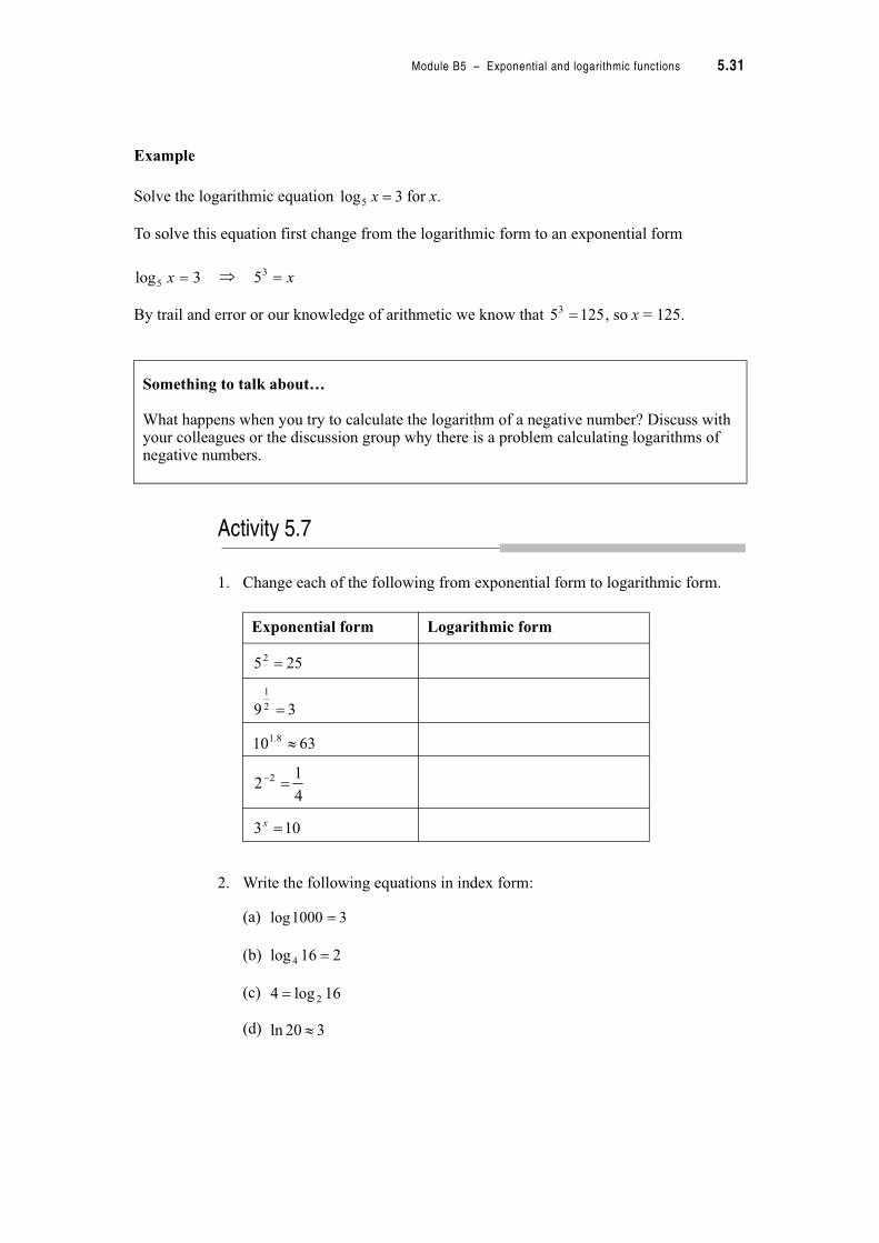
1. Change each of the following from exponential form to logarithmic form.
2. Write the following equations in index form:
(a)
(b)
(c)
(d)
Something to talk about…
What happens when you try to calculate the logarithm of a negative number? Discuss with your colleagues or the discussion group why there is a problem calculating logarithms of negative numbers.
Exponential form Logarithmic form
3log5 !x
3log5 !x x!35
12553!
2552!
39 2
1
!
6310 8.1$
4
12 2
!"
103 !x
31000log !
216log 4 !
16log4 2!
320ln $
5.32 TTPP7182 – Mathematics tertiary preparation level B
3. Use your knowledge of logarithms to evaluate:
(a) log(1 000 000)
(b)
4. Evaluate and
5. Solve the following equations for x:
(a)
(b)
(c)
(d)
(e)
5.2.2 Properties of logarithms
From our work above it appears that logarithms are really powers in a different form. So it might follow that some of the properties that apply to powers might be used to help develop some similar properties for logarithms. If you have forgotten the index laws from module 3 now would be a good time to revise them.
Before examining the properties let’s think about the relationship between indices and logarithms in more detail.
When we multiply two numbers which are in index form we add the indices, so
But logarithms are really indices, so
can be written as
Now
We can now see that
This is really a special case of our first property below. Many of the other properties are based on this relationship.
Evaluate logarithms.
Write 7 in its logarithmic form.
Write 10000000 as a product.
8
1log2
5log 25 2log 0.25
10log!x
5log 2 !x
0log 4 !x
327log "!x
3ln !x
743 101010 !
1000000010 and 1000010 and 100010 743!!!
710000000log and 410000log and 31000log 101010 !!!
)100001000(log
10000000log
7
4310000log1000log
10
10
1010
!
!
!
'!'
10000000log10000log1000log 101010 !
Module B5 – Exponential and logarithmic functions 5.33
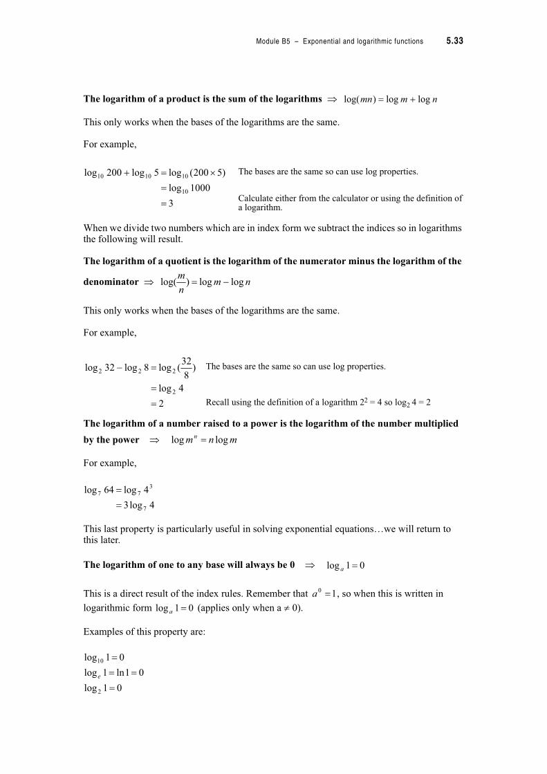
The logarithm of a product is the sum of the logarithms "
This only works when the bases of the logarithms are the same.
For example,
When we divide two numbers which are in index form we subtract the indices so in logarithms the following will result.
The logarithm of a quotient is the logarithm of the numerator minus the logarithm of the
denominator "
This only works when the bases of the logarithms are the same.
For example,
The logarithm of a number raised to a power is the logarithm of the number multiplied
by the power "
For example,
This last property is particularly useful in solving exponential equations…we will return to this later.
The logarithm of one to any base will always be 0 "
This is a direct result of the index rules. Remember that , so when this is written in
logarithmic form (applies only when a #$0).
Examples of this property are:
The bases are the same so can use log properties.
Calculate either from the calculator or using the definition of a logarithm.
The bases are the same so can use log properties.
Recall using the definition of a logarithm 22 = 4 so log2 4 = 2
nmmn loglog)log( !
3
1000log
)5200(log5log200log
10
101010
% !
nmn
mloglog)log( &
2
4log
)8
32(log8log32log
2
222
&
mnmn loglog
4log3
4log64log
7
377
01log a
10 a
01log a
01log
01ln1log
01log
2
10
e
5.34 TTPP7182 – Mathematics tertiary preparation level B
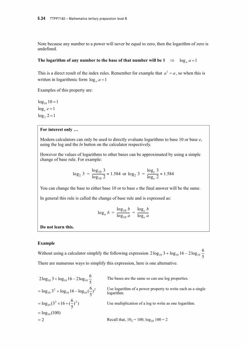
Note because any number to a power will never be equal to zero, then the logarithm of zero is undefined.
The logarithm of any number to the base of that number will be 1 "
This is a direct result of the index rules. Remember for example that , so when this is
written in logarithmic form
Examples of this property are:
Example
Without using a calculator simplify the following expression
There are numerous ways to simplify this expression, here is one alternative.
For interest only …
Modern calculators can only be used to directly evaluate logarithms to base 10 or base e, using the log and the ln button on the calculator respectively.
However the values of logarithms to other bases can be approximated by using a simple change of base rule. For example:
or
You can change the base to either base 10 or to base e the final answer will be the same.
In general this rule is called the change of base rule and is expressed as:
Do not learn this.
The bases are the same so can use log properties.
Use logarithm of a power property to write each as a single logarithm.
Use multiplication of a log to write as one logarithm.
Recall that, 102 = 100, log10 100 = 2
1log aa
aa 1
1log aa
12log
1log
110log
2
10
ee
log2 3log10 3
log10 2----------------- 1.584'= log2 3
loge 3
loge 2--------------- 1.584'=
loga blog10 b
log10 a-----------------
loge b
loge a---------------= =
5
6log216log3log2 101010 &!
2
)100(log
))5
6(163(log
)5
6(log16log3log
5
6log216log3log2
10
2210
21010
210
101010
(%
&!
&!
Module B5 – Exponential and logarithmic functions 5.35
Example
Without using a calculator write the following expression as a single logarithm or number
There are numerous ways to simplify this expression, here is one alternative.
Example
Use the definition of the logarithm and its properties to solve the following equation
Check: When
Solution is
The bases are the same so can use log properties.
Recall that because 51 = 5, log5 5 = 1
The bases are the same so can use log properties.
Use log property to write as a single logarithm.
Use logarithm in an exponential form.
04.0log125log25log 555 &!
7
5log7
5log25log35log2
5log25log35log2
5log5log35log2
25
1log5log5log
04.0log125log25log
5
555
555
2555
53
52
5
555
!!
&&!
&!
&!
&!
&
13log)2(log 1010 !&x
3
15or
3
16
23
10
3
10)2(
10)2(3
10)2(3
1]3)2[(log
13log)2(log
1
10
1010
!
&
&
&
%&
!&
x
x
x
x
x
x
x
RHS110log)33
10(log3log
3
10log3log)2
3
16(logLHS ,
3
16101010101010 % ! !& x
3
16 x
5.36 TTPP7182 – Mathematics tertiary preparation level B
Activity 5.8
1. Without using a calculator simplify the following expressions:
(a)
(b)
(c)
2. Find the value of each of the following in simplest form.
(a)
(b) ln25 + 2ln0.2
(c)
3. Use the logarithmic properties to solve the equations below.
(a)
(b) log5m = 2logm
(c)
(d) log2 + log5 + logy – log3 = 2
3
1log27log 33 !
8log16log 22 &
4log32log125log &!
2log43log2 1212 !
10log2log310log4 555 &&
2log4loglog 333 ! x
0log3log2 5 &! pp
A bit of history… For interest only
Today to many of us logarithms appear to be the most perverse and artificial of mathematical functions. But when they were invented they were thought to be the washing machine of the 17th century in that they saved many professionals from the drudgery of long multiplication and division, especially in the field of astronomy. The idea was first developed by John Napier in about 1594 and perfected by Henry Briggs in 1614. The idea is simple:
If you want to multiply two numbers, say 2376 and 34678 first write them as a power to the base of ten (this is logarithm), then instead of multiplying the numbers we can add the indices.
(Actual answer on a calculator is 82394928)
If you went to secondary school in Australia before the mid 1970s you might remember doing this with logarithm tables or a slide rule. Log Tables were books in which every number was written as a power of 10 or power of e.
Today we have calculators to do this job but logarithms are now seen to be very useful in their own right, see case studies below. Do not learn this.
82394928
10
10
1010346782376
1034678,102376
.....9160.7
....5401.4....3759.3
....5401.4....3759.3
....5400.4....3759.3
% %
!

Module B5 – Exponential and logarithmic functions 5.37
5.2.3 The function and its graph
Let’s now examine the logarithmic function, , in its own right.
To help us understand the shape of this function in more detail, use your calculator to complete
the table of values below and use it to sketch the function .
How did you go? Did you get a graph something like this?
Think about the shape, the domain and range of the curve and describe in your own words the characteristics of this logarithmic function.
__________________________________________________________________________
__________________________________________________________________________
__________________________________________________________________________
__________________________________________________________________________
__________________________________________________________________________
x
10
9
8
7
6
5
4
3
2
1
0.1
0.001
0.0001
0.00001
xy 10log
xy 10log
x10log
x
x
y
4 6 8
−2
−1
0 2
1
2
y =log 10
5.38 TTPP7182 – Mathematics tertiary preparation level B
Important characteristics of the graph you might have noticed are:
• it is a function because there is only one value of the dependent variable for each independent variable
• its domain is restricted and includes only real numbers greater than zero
• the range of each function is unrestricted and includes all real numbers
• the horizontal intercept is one
• as the independent variable decreases (approaches zero) the dependent variable approaches negative infinity
• as the independent variable increases (approaches infinity) the dependent variable increases slowly.
You should notice two things:
1. Compare this function with the inverse of the exponential function drawn at 5.1.5. They are identical. The logarithmic function is an inverse of the exponential growth function so all of its properties are mirror images of the properties of the growth function e.g. domain, range etc.
2. The vertical axis is an asymptote.
Activity 5.9
1. Sketch the graph of , in the domain 0 < x < 3
2. (a) On your graph of sketch the graphs
(i)
(ii)
(b) What effect does multiplying by 2 or adding 2 have on the shape and position of the logarithmic function?
5.2.4 Case studies
Logarithms are used to model a range of situations that occur in science, economics and engineering. They are used in isolation or in combination with other functions. For example,
In mechanical technology, belt friction in a pulley system is modelled by , where
T are the large and small tensions in the rope on the pulley, is the angle of wrap of the rope
around the pulley and is the coefficient of friction.
xy ln
xy ln
xy ln2
xy ln2 !
)* )ln(S
L
T
T
*
)
Module B5 – Exponential and logarithmic functions 5.39
In chemistry, time of reaction (t) and concentration of a substance (x) are related by the
equation, , where the k values are all constants.
In economics the growth of an economy could be represented by the formula, ,
where t is time and x the value in dollars.
However, by far the most common use of the logarithmic function is in the development of measurement scales. This application of the function makes use of the fact that as the independent variable increases there are only small changes to the dependent variable. This characteristic gives us the ability to work with very large and very small numbers more manageably within the one function. The following case studies emphasize this characteristic.
Measuring loudness
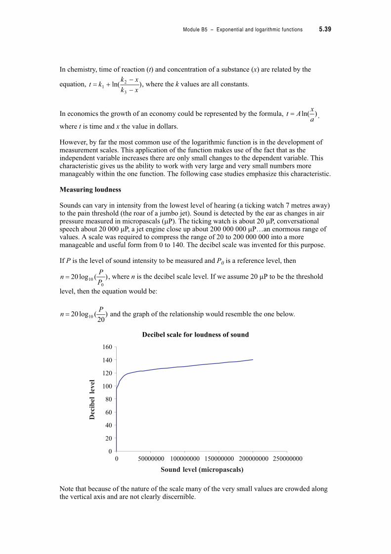
Sounds can vary in intensity from the lowest level of hearing (a ticking watch 7 metres away) to the pain threshold (the roar of a jumbo jet). Sound is detected by the ear as changes in air pressure measured in micropascals ()P). The ticking watch is about 20 )P, conversational speech about 20 000 )P, a jet engine close up about 200 000 000 )P…an enormous range of values. A scale was required to compress the range of 20 to 200 000 000 into a more manageable and useful form from 0 to 140. The decibel scale was invented for this purpose.
If P is the level of sound intensity to be measured and P0 is a reference level, then
, where n is the decibel scale level. If we assume 20 )P to be the threshold
level, then the equation would be:
and the graph of the relationship would resemble the one below.
Decibel scale for loudness of sound
Note that because of the nature of the scale many of the very small values are crowded along the vertical axis and are not clearly discernible.
)ln(3
21
xk
xkkt
&
&!
)ln(a
xAt
)(log200
10P
Pn
)20
(log20 10
Pn
0
20
40
60
80
100
120
140
160
0 50000000 100000000 150000000 200000000 250000000
Decibellevel
Sound level (micropascals)
5.40 TTPP7182 – Mathematics tertiary preparation level B
Measuring acidity
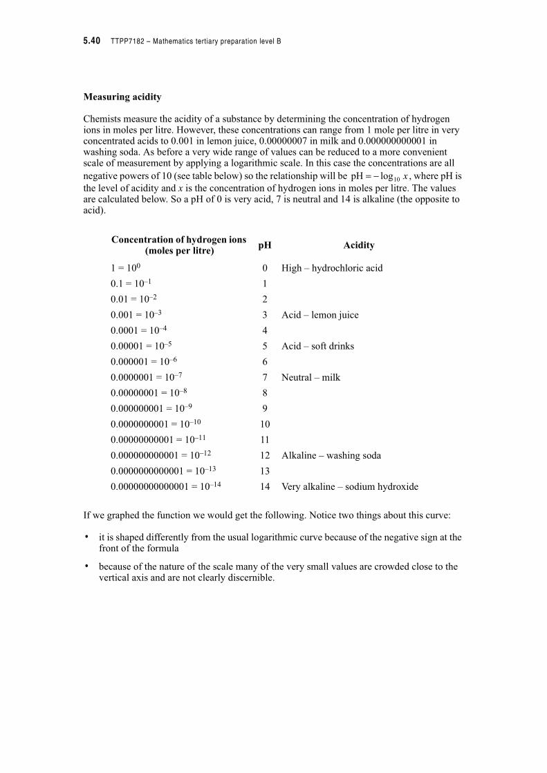
Chemists measure the acidity of a substance by determining the concentration of hydrogen ions in moles per litre. However, these concentrations can range from 1 mole per litre in very concentrated acids to 0.001 in lemon juice, 0.00000007 in milk and 0.000000000001 in washing soda. As before a very wide range of values can be reduced to a more convenient scale of measurement by applying a logarithmic scale. In this case the concentrations are all
negative powers of 10 (see table below) so the relationship will be , where pH is
the level of acidity and x is the concentration of hydrogen ions in moles per litre. The values are calculated below. So a pH of 0 is very acid, 7 is neutral and 14 is alkaline (the opposite to acid).
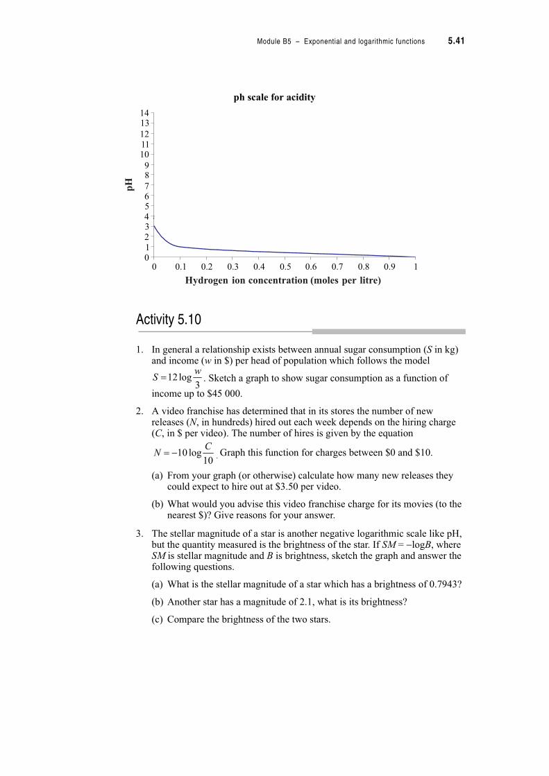
If we graphed the function we would get the following. Notice two things about this curve:
• it is shaped differently from the usual logarithmic curve because of the negative sign at the front of the formula
• because of the nature of the scale many of the very small values are crowded close to the vertical axis and are not clearly discernible.
Concentration of hydrogen ions (moles per litre)
pH Acidity
1 = 100 0 High – hydrochloric acid
0.1 = 10–1 1
0.01 = 10–2 2
0.001 = 10–3 3 Acid – lemon juice
0.0001 = 10–4 4
0.00001 = 10–5 5 Acid – soft drinks
0.000001 = 10–6 6
0.0000001 = 10–7 7 Neutral – milk
0.00000001 = 10–8 8
0.000000001 = 10–9 9
0.0000000001 = 10–10 10
0.00000000001 = 10–11 11
0.000000000001 = 10–12 12 Alkaline – washing soda
0.0000000000001 = 10–13 13
0.00000000000001 = 10–14 14 Very alkaline – sodium hydroxide
x10logpH &
Module B5 – Exponential and logarithmic functions 5.41
ph scale for acidity
Activity 5.10
1. In general a relationship exists between annual sugar consumption (S in kg) and income (w in $) per head of population which follows the model
. Sketch a graph to show sugar consumption as a function of
income up to $45 000.
2. A video franchise has determined that in its stores the number of new releases (N, in hundreds) hired out each week depends on the hiring charge (C, in $ per video). The number of hires is given by the equation
. Graph this function for charges between $0 and $10.
(a) From your graph (or otherwise) calculate how many new releases they could expect to hire out at $3.50 per video.
(b) What would you advise this video franchise charge for its movies (to the nearest $)? Give reasons for your answer.
3. The stellar magnitude of a star is another negative logarithmic scale like pH, but the quantity measured is the brightness of the star. If SM = &logB, where SM is stellar magnitude and B is brightness, sketch the graph and answer the following questions.
(a) What is the stellar magnitude of a star which has a brightness of 0.7943?
(b) Another star has a magnitude of 2.1, what is its brightness?
(c) Compare the brightness of the two stars.
0
1
2
3
4
5
6
7
8
9
10
11
12
13
14
pH
0
7
1
8
2
9
3
10
4
11
5
12
6
1314
0 0.1 0.2 0.3 0.4 0.5 0.6 0.7 0.8 0.9 1
pH
Hydrogen ion concentration (moles per litre)
3log12
wS
10log10
CN &
5.42 TTPP7182 – Mathematics tertiary preparation level B
5.2.5 Average rate of change
We can get an estimate of the rate of change of the logarithmic function just the same as we would measure the average rate of change of any curved function. Let’s have a look at some of the examples above.
Example
Determine the average rate of change in the function , between the values of x = 1
and x = 5.
This question requires us to calculate the average rate of change of the function between the values of 1 and 5. To do this we need to find the gradient of the straight line joining the points where x = 1 and x = 5.
Recall that gradient is change in the height divided by the change in the horizontal distance,
The rate of change between 1 and 5 is 0.4. This means that for every 1 unit change in the x value the y value changes by 0.4 units.
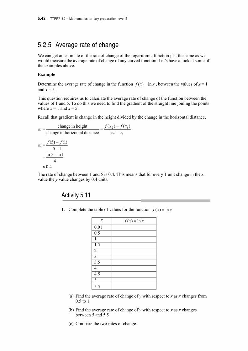
Activity 5.11
1. Complete the table of values for the function
(a) Find the average rate of change of y with respect to x as x changes from 0.5 to 1
(b) Find the average rate of change of y with respect to x as x changes between 5 and 5.5
(c) Compare the two rates of change.
x
0.01
0.5
1
1.5
2
3
3.5
4
4.5
5
5.5
xxf ln)(
12
12 )()(
distance horizontalin change
heightin change
xx
xfxfm
&
&
4.0
4
1ln5ln
15
)1()5(
'
&
&
&
ffm
xxf ln)(
xxf ln)(
Module B5 – Exponential and logarithmic functions 5.43
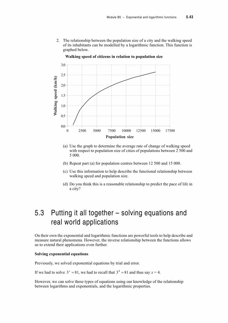
2. The relationship between the population size of a city and the walking speed of its inhabitants can be modelled by a logarithmic function. This function is graphed below.
Walking speed of citizens in relation to population size
(a) Use the graph to determine the average rate of change of walking speed with respect to population size of cities of populations between 2 500 and 5 000.
(b) Repeat part (a) for population centres between 12 500 and 15 000.
(c) Use this information to help describe the functional relationship between walking speed and population size.
(d) Do you think this is a reasonable relationship to predict the pace of life in a city?
5.3 Putting it all together – solving equations and
real world applications
On their own the exponential and logarithmic functions are powerful tools to help describe and measure natural phenomena. However, the inverse relationship between the functions allows us to extend their applications even further.
Solving exponential equations
Previously, we solved exponential equations by trial and error.
If we had to solve , we had to recall that and thus say x = 4.
However, we can solve these types of equations using our knowledge of the relationship between logarithms and exponentials, and the logarithmic properties.
0.0
0.5
1.0
1.5
2.0
2.5
3.0
0 2500 5000 7500 10000 12500 15000 17500
Walkingspeed(km/h)
Population size
813 x 8134
5.44 TTPP7182 – Mathematics tertiary preparation level B
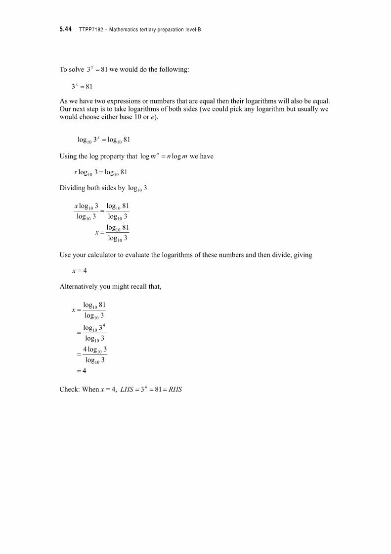
To solve we would do the following:
As we have two expressions or numbers that are equal then their logarithms will also be equal. Our next step is to take logarithms of both sides (we could pick any logarithm but usually we would choose either base 10 or e).
Using the log property that we have
Dividing both sides by
Use your calculator to evaluate the logarithms of these numbers and then divide, giving
x = 4
Alternatively you might recall that,
Check: When x = 4,
813 x
813 x
81log3log 1010 x
mnm n loglog
81log3log 1010 x
3log10
3log
81log
3log
81log
3log
3log
10
10
10
10
10
10
x
x
4
3log
3log4
3log
3log
3log
81log
10
10
10
410
10
10
x
RHSLHS 8134
Module B5 – Exponential and logarithmic functions 5.45
Example
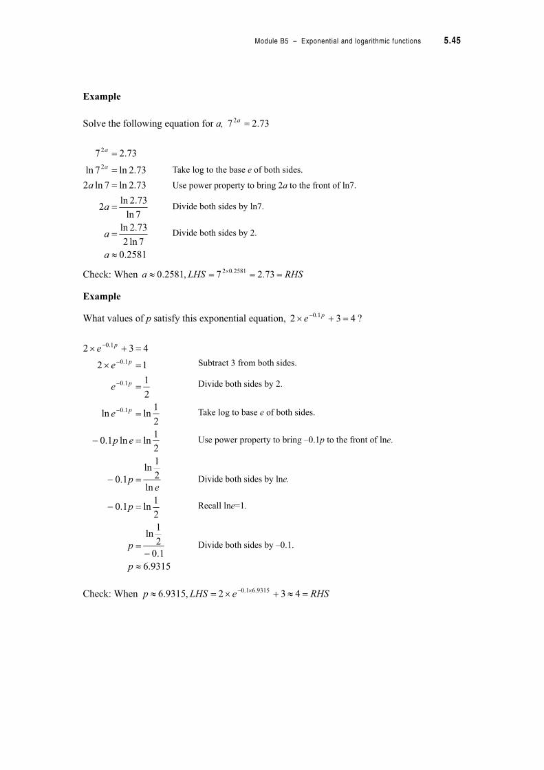
Solve the following equation for a,
Check: When
Example
What values of p satisfy this exponential equation, ?
Check: When
Take log to the base e of both sides.
Use power property to bring 2a to the front of ln7.
Divide both sides by ln7.
Divide both sides by 2.
Subtract 3 from both sides.
Divide both sides by 2.
Take log to base e of both sides.
Use power property to bring –0.1p to the front of lne.
Divide both sides by lne.
Recall lne=1.
Divide both sides by –0.1.
73.27 2 a
2581.0
7ln2
73.2ln
7ln
73.2ln2
73.2ln7ln2
73.2ln7ln
73.27
2
2
'
a
a
a
a
a
a
RHSLHSa '% 73.27,2581.0 2581.02
432 1.0 !% & pe
9315.6
1.0
2
1ln
2
1ln1.0
ln
2
1ln
1.0
2
1lnln1.0
2
1lnln
2
1
12
432
1.0
1.0
1.0
1.0
'
&
&
&
&
%
!%
&
&
&
&
p
p
p
ep
ep
e
e
e
e
p
p
p
p
RHSeLHSp '!% ' %& 432,9315.6 9315.61.0
5.46 TTPP7182 – Mathematics tertiary preparation level B
Example
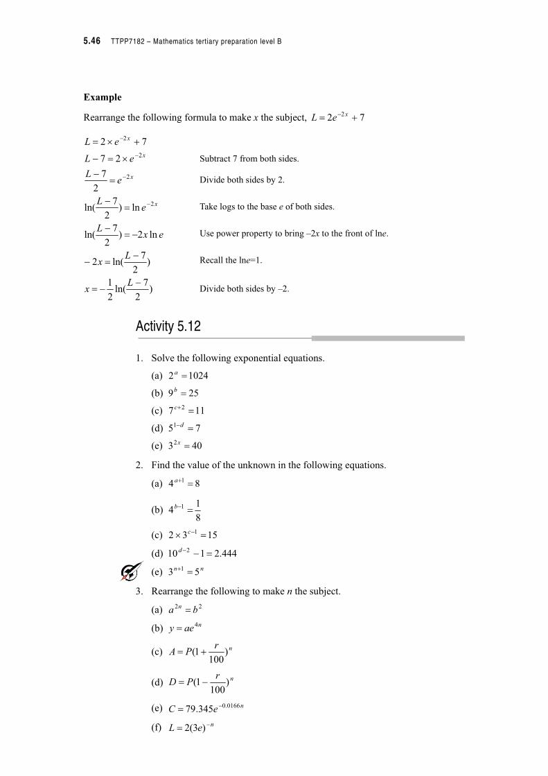
Rearrange the following formula to make x the subject,
Activity 5.12
1. Solve the following exponential equations.
(a)
(b)
(c)
(d)
(e)
2. Find the value of the unknown in the following equations.
(a)
(b)
(c)
(d)
(e)
3. Rearrange the following to make n the subject.
(a)
(b)
(c)
(d)
(e)
(f)
Subtract 7 from both sides.
Divide both sides by 2.
Take logs to the base e of both sides.
Use power property to bring –2x to the front of lne.
Recall the lne=1.
Divide both sides by –2.
72 2 ! & xeL
)2
7ln(
2
1
)2
7ln(2
ln2)2
7ln(
ln)2
7ln(
2
7
27
72
2
2
2
2
&&
& &
& &
&
&
% &
!%
&
&
&
&
Lx
Lx
exL
eL
eL
eL
eL
x
x
x
x
10242 a
259 b
117 2 !c
751 &d
4032 x
84 1 !a
8
14 1 &b
1532 1 % &c
444.2110 2 &&d
nn 53 1 !
22 ba n
naey 4
nrPA )
1001( !
nrPD )
1001( !
neC 0166.0345.79 !
neL ! )3(2
Module B5 – Exponential and logarithmic functions 5.47
Real world applications
This section will examine some real world applications which require solution of exponential equations.
Example
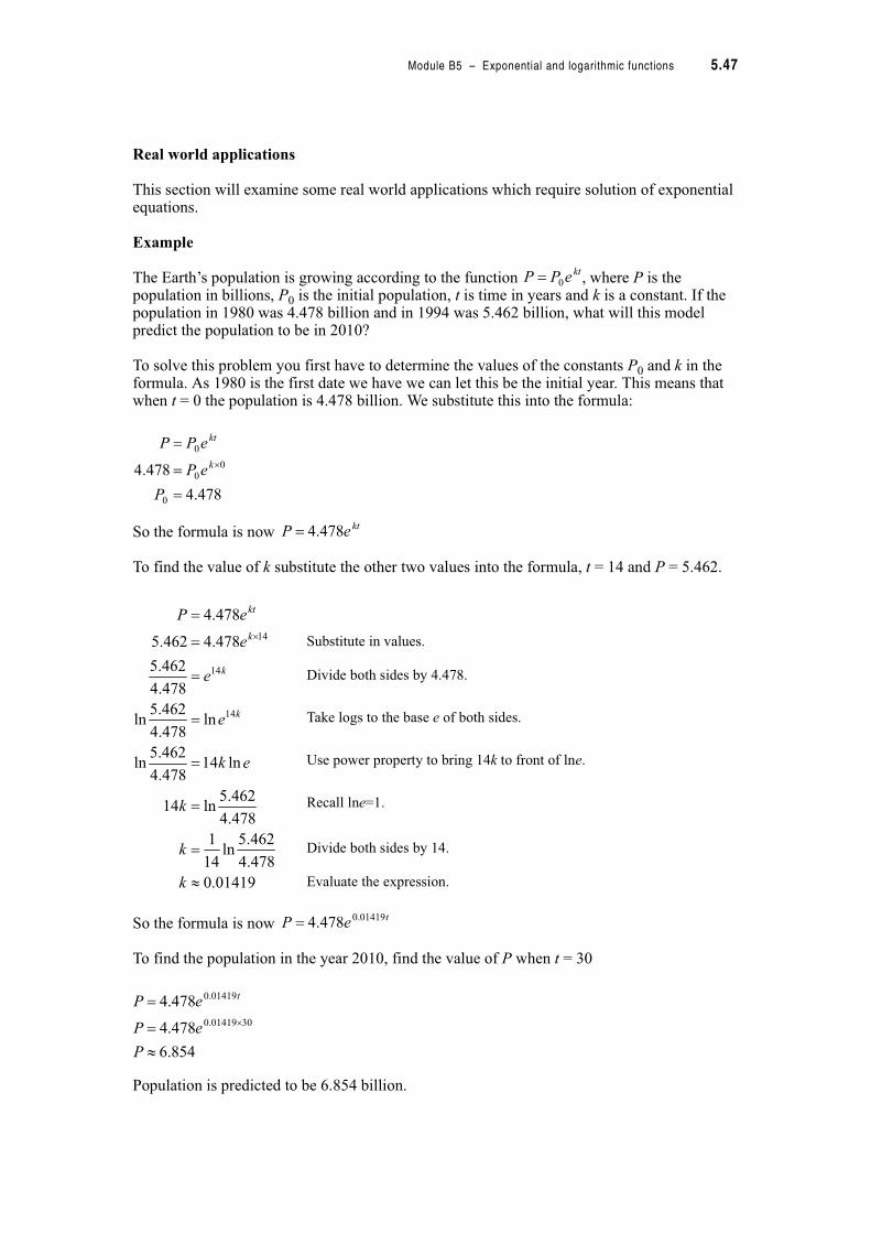
The Earth’s population is growing according to the function , where P is the population in billions, P0 is the initial population, t is time in years and k is a constant. If the population in 1980 was 4.478 billion and in 1994 was 5.462 billion, what will this model predict the population to be in 2010?
To solve this problem you first have to determine the values of the constants P0 and k in the formula. As 1980 is the first date we have we can let this be the initial year. This means that when t = 0 the population is 4.478 billion. We substitute this into the formula:
So the formula is now
To find the value of k substitute the other two values into the formula, t = 14 and P = 5.462.
So the formula is now
To find the population in the year 2010, find the value of P when t = 30
Population is predicted to be 6.854 billion.
Substitute in values.
Divide both sides by 4.478.
Take logs to the base e of both sides.
Use power property to bring 14k to front of lne.
Recall lne=1.
Divide both sides by 14.
Evaluate the expression.
ktePP 0!
478.4
478.4
0
00
0
!
!
!
"
P
eP
ePP
k
kt
kteP 478.4!
01419.0
478.4
462.5ln
14
1
478.4
462.5ln14
ln14478.4
462.5ln
ln478.4
462.5ln
478.4
462.5
478.4462.5
478.4
14
14
14
#
!
!
!
!
!
!
!
"
k
k
k
ek
e
e
e
eP
k
k
k
kt
teP 01419.0478.4!
854.6
478.4
478.4
3001419.0
01419.0
#
!
!
"
P
eP
eP t
5.48 TTPP7182 – Mathematics tertiary preparation level B
Example
Radioactive decay is modelled by the equation , where N represents the mass of the substance, N0 the initial mass of the substance and t the time. If a certain radioactive substance has a half-life of 5 years and 20 grams of it was initially secured, how much of the substance would be left after 10 years? If the substance could only be safely moved in batches of 0.1 g, when would the original 20 g be safe to move?
This first step in the solution of this question is to determine the value of k. We know that we started with 20 g so N0 = 20, we know that in 5 years we only have half of this (10 g) so N = 10 when t = 5.
So using our model we get,
Now that we know the value of k we can determine the amount of the substance left after 10 years.
There would be approximately 5 g left after 10 years.
kteNN ! 0
138629.0
5
5.0ln
5)5.0ln(
ln5)5.0ln(
)ln()5.0ln(
5.0
2010
5
5
5
0
#
!
!
!
!
!
!
!
k
k
k
ek
e
e
e
eNN
k
k
k
kt
5
20
20
38629.1
10138629.0
#
!
!
"
e
eN
Module B5 – Exponential and logarithmic functions 5.49
We can also determine how long it would take to have decayed to 0.1 g of the substance.
It would be safe to transport the substance after 38.22 years.
Activity 5.13
1. The growth function models the amount to which $P grows in t years at an interest rate of k% compounded continuously. At the current rate $100 will grow to $185 in 10 years. What would it amount to in 20 years?
2. A radioactive material is decaying exponentially. If N0 is the initial mass of
the material, N the mass at any time t and k the rate of decay, then the function
is modelled by the equation . It takes 2 years for 100 g of the
material to reduce to 60 g. How long would it take the same mass to reduce to 30 g?
3. The present temperature of a star is 10 000$C, and it is losing heat continuously in such a way that its temperature T in t million years may be
obtained from the decay function . If the temperature has halved
after 5 million years what will its temperature be in 10 million years?
4. The number of bacteria in a culture was initially 2 000. The number increases
exponentially at the rate k% per hour for t hours, i.e. . After 2 hours
the number present is 2 420. How many will be present after 24 hours?
5. The population of a city grew exponentially ( ) from 120 000 to 180 000 over a period of 10 years. How long before it reaches 200 000?
Something to talk about...
This module contains some new and different concepts. Share with the discussion group your technique for coming to terms with the concept of logarithms.
22.38
138629.0
)20
1.0ln(
138629.0)20
1.0ln(
ln138629.0)20
1.0ln(
ln)20
1.0ln(
20
1.0
201.0
138629.0
138629.0
138629.0
#
!
!
!
!
!
!
t
t
t
et
e
e
e
t
t
t
ktPeA !
kteNN ! 0
kteTT ! 0
kteNN 0!
ktePP 0!
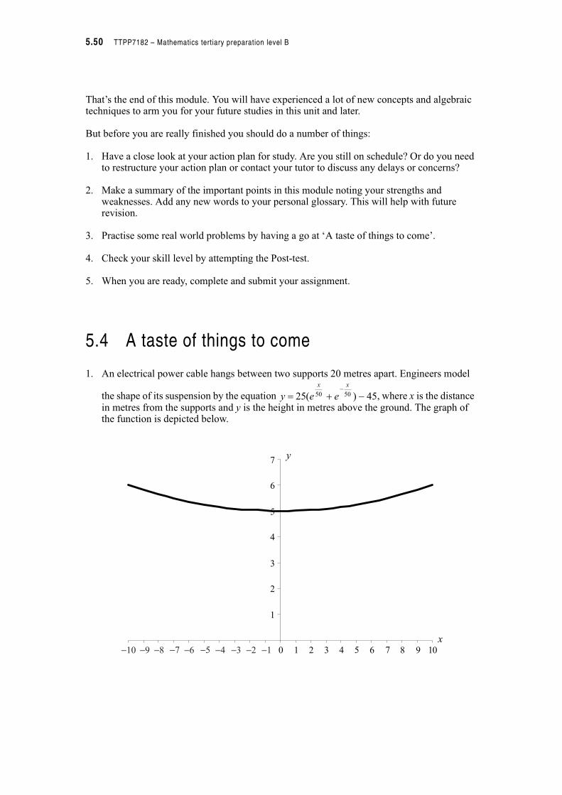
5.50 TTPP7182 – Mathematics tertiary preparation level B
That’s the end of this module. You will have experienced a lot of new concepts and algebraic techniques to arm you for your future studies in this unit and later.
But before you are really finished you should do a number of things:
1. Have a close look at your action plan for study. Are you still on schedule? Or do you need to restructure your action plan or contact your tutor to discuss any delays or concerns?
2. Make a summary of the important points in this module noting your strengths and weaknesses. Add any new words to your personal glossary. This will help with future revision.
3. Practise some real world problems by having a go at ‘A taste of things to come’.
4. Check your skill level by attempting the Post-test.
5. When you are ready, complete and submit your assignment.
5.4 A taste of things to come
1. An electrical power cable hangs between two supports 20 metres apart. Engineers model
the shape of its suspension by the equation , where x is the distance in metres from the supports and y is the height in metres above the ground. The graph of the function is depicted below.
45)(25 5050 %!
xx
eey
1
2
3
4
5
6
7
0 1 2 3 4 5 6 7 8 9 10
y
x−10 −9 −8 −7 −6 −5 −4 −3 −2 −1

Module B5 – Exponential and logarithmic functions 5.51
(a) How much does the cable sag?
(b) Engineers need to know the slope of cable where it attaches to each pylon. Find the approximate value of this by finding the average slope of the cable 1 metre from the support?
(c) What is the average slope of the cable 1 metre from the lowest point?
2. In environmental studies researchers are interested in the concept of carrying capacity and population growth. Carrying capacity is the maximum population that can be supported in a particular environment. Growth rates are often modelled to include this variable.
In practice mice populations do not grow exponentially because of the limits of food and other
resources. It could follow the model , where t is time in weeks and N the
number of mice. The function looks like this.
Size of mouse population over time
(a) On the axes above sketch a graph of the traditional exponential model , where N0 is 50 mice and a is 0.24.
(b) Comment on the graphs of the two models.
(c) Compare the populations predicted by the two models after 30 weeks.
t
t
e
eN
24.0
24.0
006.01
50
%!
00 1 8 9 10 11 12 132 3 4 5 6 7
100
200
300
400
500
600
700
800
900
Time (weeks)
Popula
tion
size
ateNN 0!
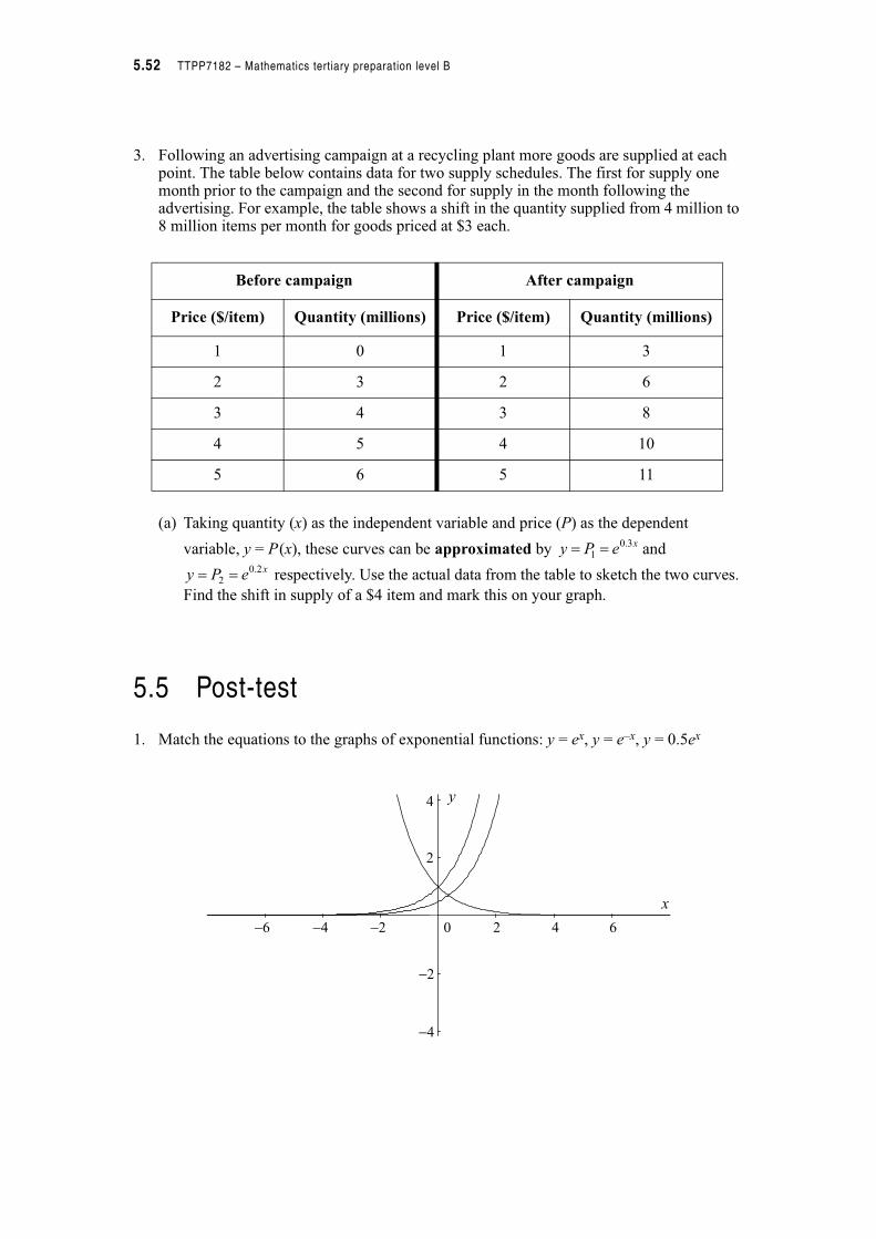
5.52 TTPP7182 – Mathematics tertiary preparation level B
3. Following an advertising campaign at a recycling plant more goods are supplied at each point. The table below contains data for two supply schedules. The first for supply one month prior to the campaign and the second for supply in the month following the advertising. For example, the table shows a shift in the quantity supplied from 4 million to 8 million items per month for goods priced at $3 each.
(a) Taking quantity (x) as the independent variable and price (P) as the dependent
variable, y = P(x), these curves can be approximated by and
respectively. Use the actual data from the table to sketch the two curves.
Find the shift in supply of a $4 item and mark this on your graph.
5.5 Post-test
1. Match the equations to the graphs of exponential functions: y = ex, y = e–x, y = 0.5ex
Before campaign After campaign
Price ($/item) Quantity (millions) Price ($/item) Quantity (millions)
1 0 1 3
2 3 2 6
3 4 3 8
4 5 4 10
5 6 5 11
xePy 3.01 !!
xePy 2.02 !!
x
y
−6 −4 −2 0 2 4 6
−4
−2
2
4
Module B5 – Exponential and logarithmic functions 5.53
2. Determine the y-intercepts for each of the following:
(a)
(b)
(c)
(d)
3. Find the value of y when x = 2 in
4. Write the following equations in logarithmic form.
(a)
(b)
5. Use your knowledge of the definition of a logarithm to evaluate:
(a)
(b)
6. Write the following equations in exponential form.
(a)
(b)
7. Determine p and q in the following equations.
(a)
(b)
8. Find t in the following equations.
(a)
(b)
9. Without using a calculator write the following expressions as a single logarithm or number.
(a)
(b)
xy )2
1(2"!
2
12 !
xy
2
12 %! xy
xy 22
1"!
xy "! )5.1(5.1
510 1 !%x
ye!2
81log3
125log
5
1
1.0log10!a
b!8log2
5)2(log 2 !p
405.010
ln !q
5.72 !t
)1(81 2te !
9log9
1log27log 333 %
2ln210ln4.0ln % ee
5.54 TTPP7182 – Mathematics tertiary preparation level B
10. Use logarithmic properties to solve:
(a)
(b)
11. What value of r satisfies this exponential equation,
12. Rearrange the following formula to make t the subject,
13. If , show that
14. If , find n in terms of A, P and i.
15. Use the formula found in Q14 for n to find how long it would take $50 (P) to amount to $75 (A) if the interest is compounded at 8.5% (i = 0.085).
16. Machinery originally costing $250 000 depreciates at 20% pa on the diminishing value.
(a) Construct a depreciation schedule (nearest $) for the first 6 years after purchase, presenting the schedule as a table and as a graph.
(b) Use the above information to write the exponential function for the depreciation value (D) as a function of time (n)
(c) Use the function to estimate its value in 10 years time.
17. The voltage (V measured in volts) across a capacitor is modelled by the equation,
, where t is measured in seconds. Find V when t = 5.
18. The function, (t measured in years, R in grams) approximates the decay of a certain element.
(a) What is its weight when t = 0?
(b) How long will it take to reduce to half its weight?
19. The function (P in billions of people and t in years) modelled Earth’s population growth in 1981. Compare the rate of growth over the years 1981 to 1986 with the expected rate of growth 20 years later, i.e. 2001 to 2006.
20. The equation can be used to convert any number of decibels (n) to the corresponding number of micropascals ( P) used to measure loudness. Show that a 60 decibel sound is 10 times as loud as a 50 decibel sound, and 100 times as loud as a 40 decibel sound.
2loglog3log 444 ! x
4
1loglog
8
1log 222 !% y
41104 100 ! "
r
34.1 6.0 !
tey
naeg )(3"!1ln
3lnln
%
!
a
gn
niPA )1( %!
310
t
eV
!
teR 075.012 !
teP 0142.05.4!
nP 1.01020"!&
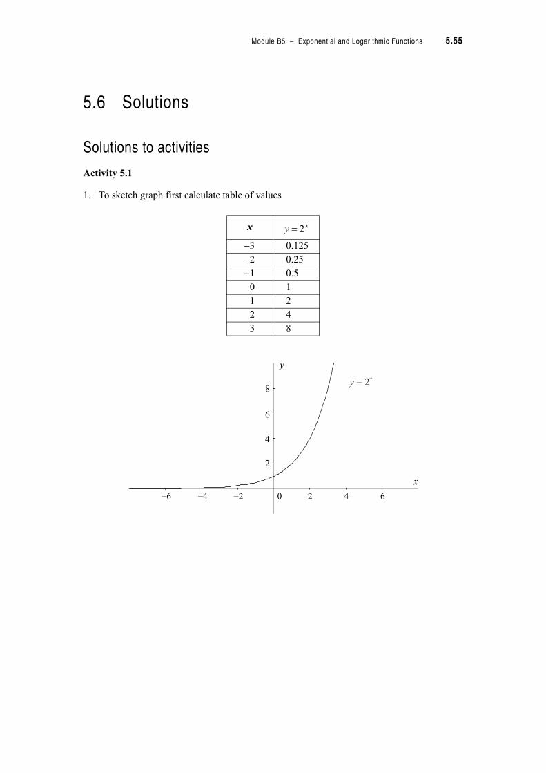
Module B5 – Exponential and Logarithmic Functions 5.55
Module B5 – Exponential and Logarithmic Functions
5.6 Solutions
Solutions to activities
Activity 5.1
1. To sketch graph first calculate table of values
x
3 0.125
2 0.25
1 0.5
0 1
1 2
2 4
3 8
xy 2!
x
y
−6 −4 −2 0 2 4 6
2
4
6
8y = 2
x
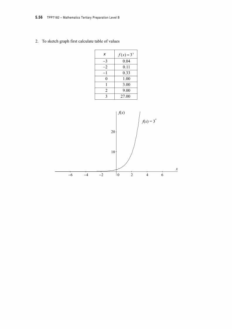
5.56 TPP7182 – Mathematics Tertiary Preparation Level B
2. To sketch graph first calculate table of values
x
3 0.04
2 0.11
1 0.33
0 1.00
1 3.00
2 9.00
3 27.00
xxf 3)( !
x
f x( )
f x( ) = 3x
−6 −4 −2 0 2 4 6
10
20
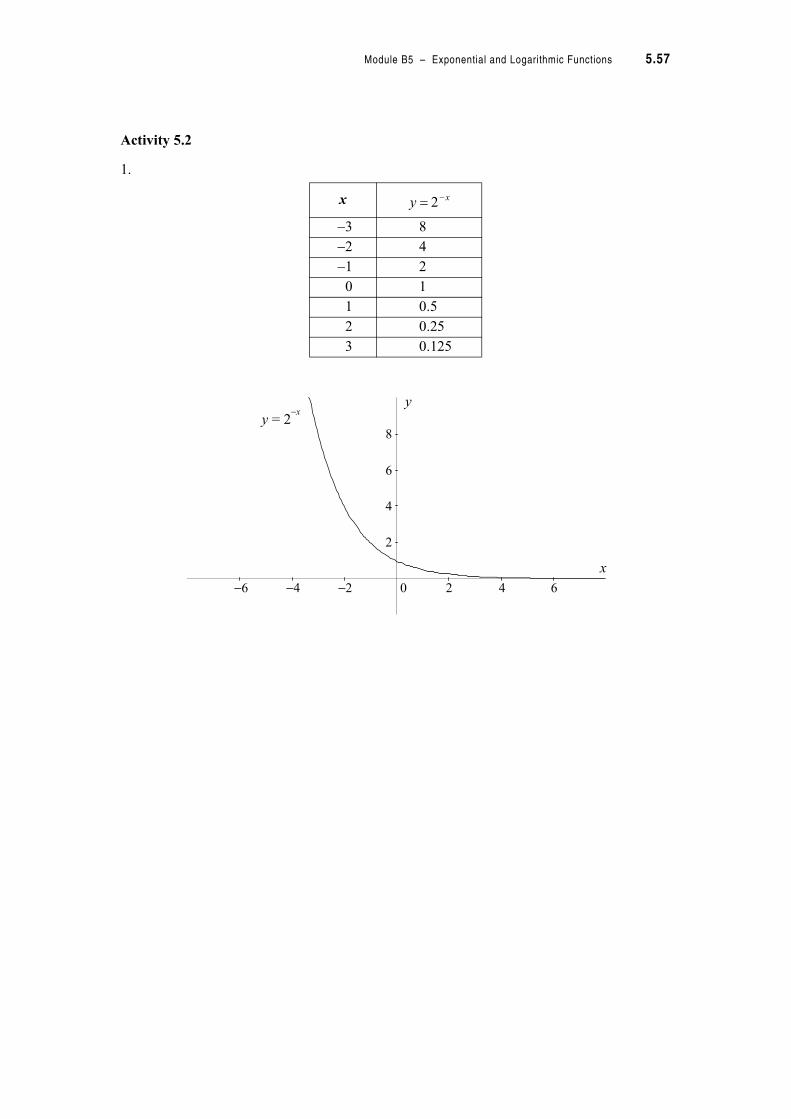
Module B5 – Exponential and Logarithmic Functions 5.57
Activity 5.2
1.
x
3 8
2 4
1 2
0 1
1 0.5
2 0.25
3 0.125
xy ! 2
x
y
y = 2−x
−6 −4 −2 0 2 4 6
2
4
6
8
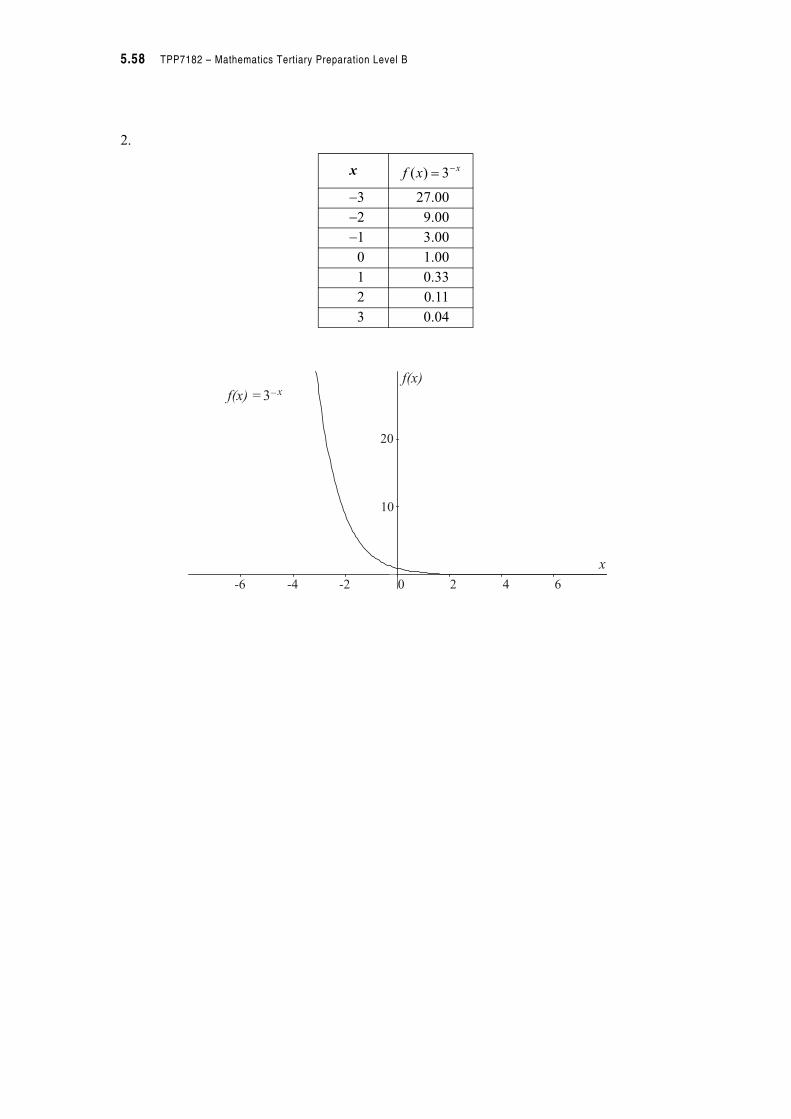
5.58 TPP7182 – Mathematics Tertiary Preparation Level B
2.
x
3 27.00
2 9.00
1 3.00
0 1.00
1 0.33
2 0.11
3 0.04
xxf ! 3)(
x
y
-6 -4 -2 0 2 4 6
10
20
f(x) =3–x
f(x)
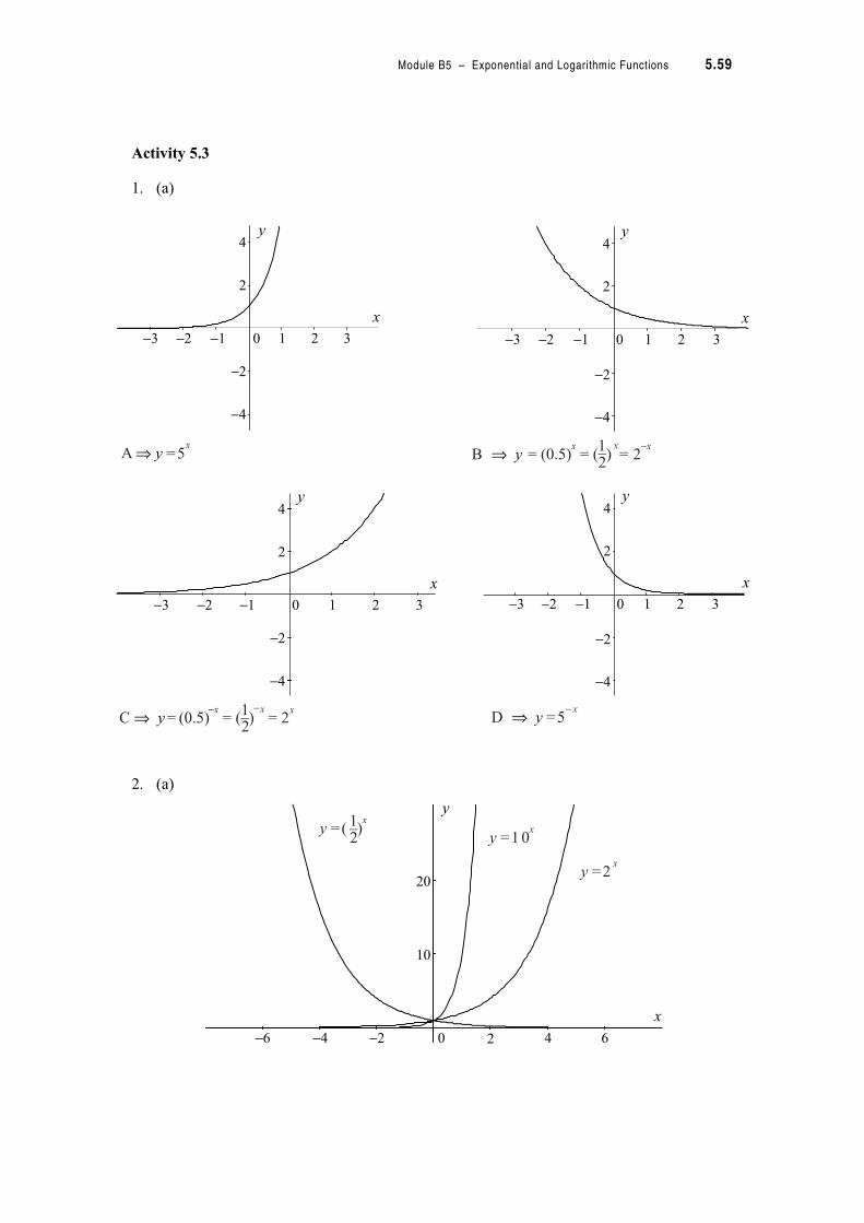
Module B5 – Exponential and Logarithmic Functions 5.59
Activity 5.3
1. (a)
2. (a)
x
x
x
x
y
y
y
y
−3
−3
−3
−3
−2
−2
−2
−2
−1
−1
−1
−1
0
0
0
0
1
1
1
1
2
2
2
2
3
3
3
3
−4
−4
−4
−4
−2
−2
−2
−2
2
2
2
2
4
4
4
4
A =5x
⇒ y
D =5− x
⇒ y
B = (0.5) = ( ) = 2−xx x
⇒ y2_1
C = (0.5) = ( ) = 2xx− −x
⇒ y2_1
x
y
−6 −4 −2 0 42 6
10
20y =2
x
y =10xy =( )
x
2_1
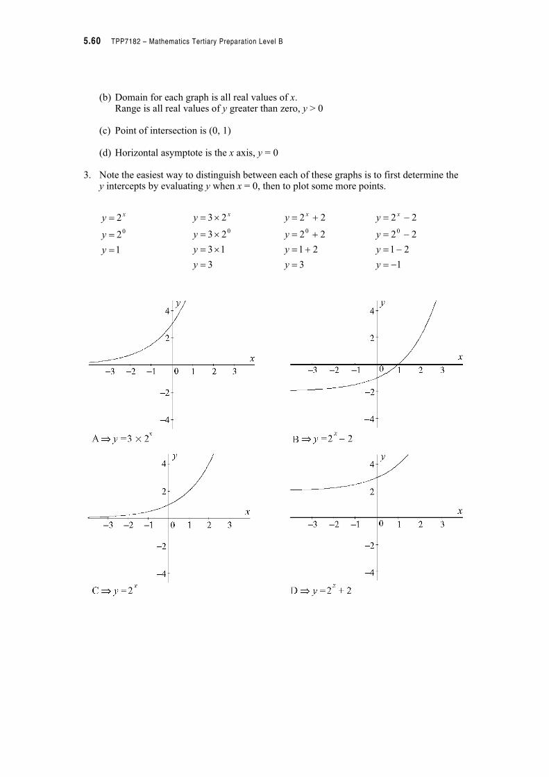
5.60 TPP7182 – Mathematics Tertiary Preparation Level B
(b) Domain for each graph is all real values of x.Range is all real values of y greater than zero, y > 0
(c) Point of intersection is (0, 1)
(d) Horizontal asymptote is the x axis, y = 0
3. Note the easiest way to distinguish between each of these graphs is to first determine they intercepts by evaluating y when x = 0, then to plot some more points.
1
2
2
0
!
!
!
y
y
y x
3
13
23
23
0
!
"!
"!
"!
y
y
y
y x
3
21
22
22
0
!
%!
%!
%!
y
y
y
y x
1
21
22
22
0
!
!
!
!
y
y
y
y x
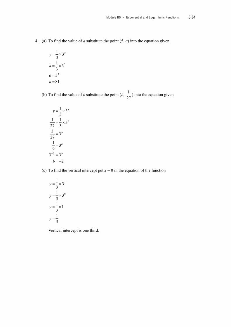
Module B5 – Exponential and Logarithmic Functions 5.61
4. (a) To find the value of a substitute the point (5, a) into the equation given.
(b) To find the value of b substitute the point (b, ) into the equation given.
(c) To find the vertical intercept put x = 0 in the equation of the function
Vertical intercept is one third.
81
3
33
1
33
1
4
5
!
!
"!
"!
a
a
a
y x
27
1
2
33
39
1
327
3
33
1
27
1
33
1
2
!
!
!
!
"!
"!
b
y
b
b
b
b
x
3
1
13
1
33
1
33
1
0
!
"!
"!
"!
y
y
y
y x
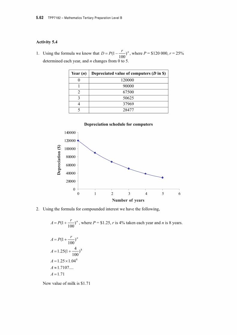
5.62 TPP7182 – Mathematics Tertiary Preparation Level B
Activity 5.4
1. Using the formula we know that , where P = $120 000, r = 25%
determined each year, and n changes from 0 to 5.
Depreciation schedule for computers
2. Using the formula for compounded interest we have the following,
, where P = $1.25, r is 4% taken each year and n is 8 years.
New value of milk is $1.71
Year (n) Depreciated value of computers (D in $)
0 120000
1 90000
2 67500
3 50625
4 37969
5 28477
nrPD )
1001( !
00 1 2 3 4 5 6
20000
40000
60000
80000
100000
120000
140000
Number of years
Dep
reci
ation
($)
nrPA )
1001( %!
71.1
....7107.1
04.125.1
)100
41(25.1
)100
1(
8
8
!
#
"!
%!
%!
A
A
A
A
rPA n

Module B5 – Exponential and Logarithmic Functions 5.63
3. We use the compound interest formula, , to calculate returns from both
packages.
Package 1: P = $90 000, r is 6.5% every 6 months so , n is for two six
month periods so is 2.
Return is $95 945.06
Package 2: P = $90 000, r is 6.4% for 365 days so , n is 365 days.
Return is $95 947.78
Melvil should take the second package as his money will have earned an extra $2.72.
4. Calculate a table of values.
Hours (t) Number of bacteria (N(t))
0 200
1 1600
2 12800
3 102400
4 819200
5 6553600
6 52428800
7 419430400
8 3355443200
9 26843545600
nrPA )
1001( %!
%25.32
%5.6!!r
06.95945
0625.95945
)0325.1(90000
)100
25.31(90000
)100
1(
2
2
#
!
!
%!
%!
A
A
A
A
rPA n
365
%4.6!r
78.95947
775.95947
...)000175.1(90000
)100
)365
4.6(
1(90000
)100
1(
365
365
#
!
!
%!
%!
A
A
A
A
rPA n
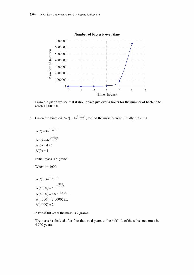
5.64 TPP7182 – Mathematics Tertiary Preparation Level B
Number of bacteria over time
From the graph we see that it should take just over 4 hours for the number of bacteria to reach 1 000 000
5. Given the function , to find the mass present initially put t = 0.
Initial mass is 4 grams.
When t = 4000
After 4000 years the mass is 2 grams.
The mass has halved after four thousand years so the half-life of the substance must be 4 000 years.
0
1000000
2000000
3000000
4000000
5000000
6000000
7000000
Time (hours)
Num
ber
of
bact
eria
43 50 1 62
)5771
(
4)(
t
etN
!
4)0(
14)0(
4)0(
4)(
)5771
0(
)5771
(
!
"!
!
!
N
N
eN
etN
t
2)4000(
...000052.2)4000(
4)4000(
4)4000(
4)(
...69312.0
)5771
4000(
)5771
(
#
!
"!
!
!
N
N
eN
eN
etN
t
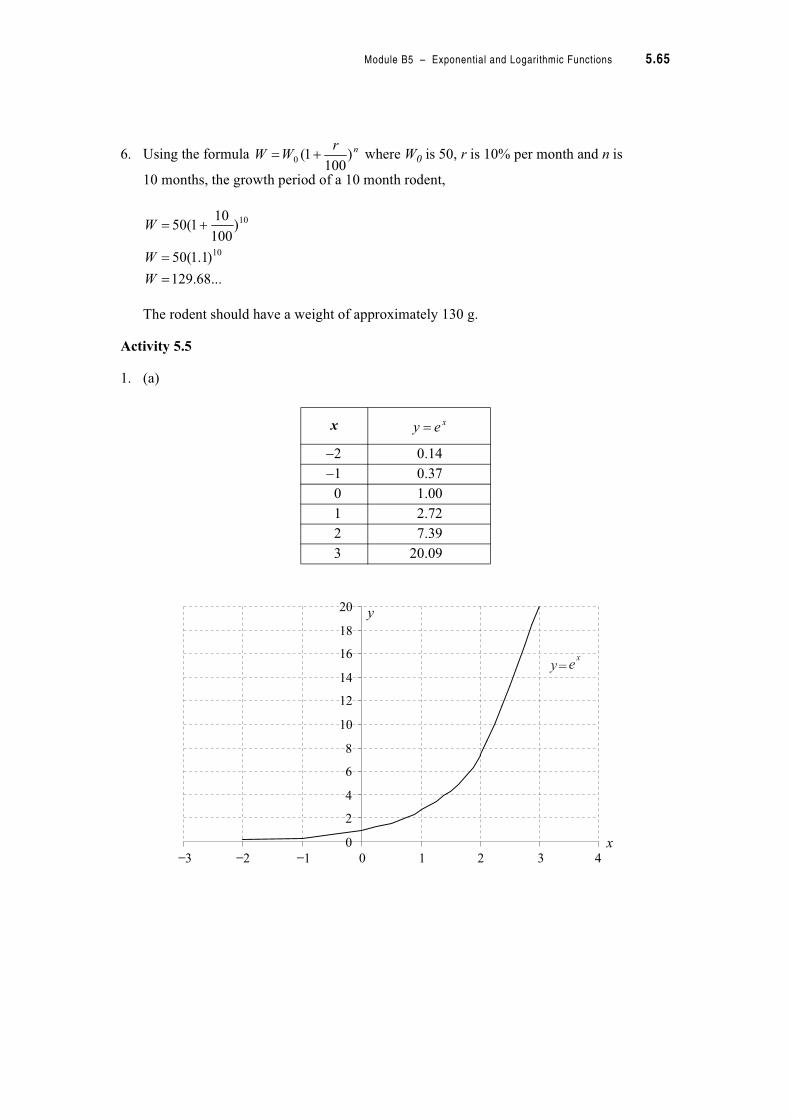
Module B5 – Exponential and Logarithmic Functions 5.65
6. Using the formula where W0 is 50, r is 10% per month and n is
10 months, the growth period of a 10 month rodent,
The rodent should have a weight of approximately 130 g.
Activity 5.5
1. (a)
x
2 0.14
1 0.37
0 1.00
1 2.72
2 7.39
3 20.09
nrWW )
1001(0 %!
...68.129
)1.1(50
)100
101(50
10
10
!
!
%!
W
W
W
xey !
0
2
4
6
8
10
12
14
16
18
20
−3 −2 −1 0 1 2 3 4
y
x
y e=x
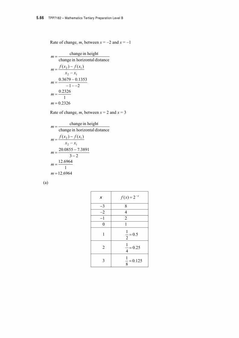
5.66 TPP7182 – Mathematics Tertiary Preparation Level B
Rate of change, m, between x = 2 and x = 1
Rate of change, m, between x = 2 and x = 3
(a)
x
3 8
2 4
1 2
0 1
1 0.5
2 0.25
3 0.125
2326.0
1
2326.0
21
1353.03679.0
)()(
distance horizontalin change
heightin change
12
12
!
!
!
!
!
m
m
m
xx
xfxfm
m
6964.12
1
6964.12
23
3891.70855.20
)()(
distance horizontalin change
heightin change
12
12
!
!
!
!
!
m
m
m
xx
xfxfm
m
xxf ! 2)(
!2
1
!4
1
!8
1
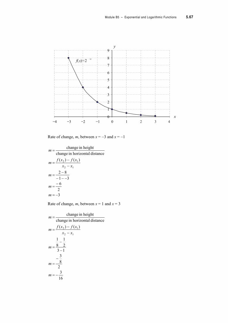
Module B5 – Exponential and Logarithmic Functions 5.67
Rate of change, m, between x = 3 and x = 1
Rate of change, m, between x = 1 and x = 3
0
1
2
3
4
5
6
7
8
9
−4 −3 −2 −1 0 1 2 3 4
x
y
f x( )=2–x
3
2
6
31
82
)()(
distance horizontalin change
heightin change
12
12
!
!
!
!
!
m
m
m
xx
xfxfm
m
16
3
2
8
3
13
2
1
8
1
)()(
distance horizontalin change
heightin change
12
12
!
!
!
!
!
m
m
m
xx
xfxfm
m

5.68 TPP7182 – Mathematics Tertiary Preparation Level B
2. (a) From the graph the approximate coordinates are (9, 40) and (10, 60) to the nearest 10.
Average gradient is 20.
(b) A range of alternatives are possible for this answer here are two.
(i) The values of y are increasing with respect to x at a rate of 20 for each unit of x.
(ii) When x increases by one unit the value of y increases 20 units.
3. The depreciation schedule for this car is as follows calculated from the formula,
where P = $32 000, r = 25% determined each year, and n changes
from 0 to 6.
Year (n)Depreciated value
(D=f(n))
0 32000
1 24000
2 18000
3 13500
4 10125
5 7594
6 5695
20
1
4060
910
)9()10(
)()(
distance horizontalin change
heightin change
12
12
!
!
!
!
!
m
m
ffm
xx
xfxfm
m
nrPnfD )
1001()( !!
Module B5 – Exponential and Logarithmic Functions 5.69
(a) Average rate of change of the value of the car over the first two years,
Value of car is decreasing in the first two years by $7000 per year.
(b) Average rate of change of the value of the car over the six years,
Value of car is decreasing in the entire six years by about $4384 per year.
4. (a) To find the rate at which the iceblock melts over the first five minutes calculate the rate
of change between t = 0 and t = 5 for the function
Block melts at a rate of –1.48 cm3 per minute. The negative sign indicates it is decreasing in volume.
7000
2
14000
2
3200018000
02
)0()2(
)()(
distance horizontalin change
heightin change
12
12
!
!
!
!
!
!
m
m
m
ffm
nn
nfnfm
m
17.4384
6
26305
06
320005695
06
)0()6(
)()(
distance horizontalin change
heightin change
12
12
#
!
!
!
!
!
m
m
m
ffm
nn
nfnfm
m
tetfV 05672.030)( !!
48.1
5
30592.22
05
)0()5(
)()(
distance horizontalin change
heightin change
12
12
#
!
!
!
!
m
m
ffm
tt
tftfm
m
5.70 TPP7182 – Mathematics Tertiary Preparation Level B
(b) To find rate at which iceblock melts over the five minutes from the 30th to 35th minute, calculate the rate of change between t = 30 and t = 35 for the function
Block melts at a rate of 0.27 cm3 per minute. The negative sign indicates it is decreasing in volume.
(c) Since the melting rate in the 30 to 35 minute time span is much slower than the melting rate in the first 5 minutes, the ice melts much more slowly as time passes, decreasing in size more slowly.
5. To find the rate of change we need to use the equation and evaluate it
for n = 4 and n = 5, n is recorded in thousands unit lots.
Thus profit increased by 2 cents per unit for each lot of thousand units produced. This means that for a thousand units the profit increases by $20.
tetfV 05672.030)( !!
27.0
5
4717.51206.4
3035
)30()35(
)()(
distance horizontalin change
heightin change
12
12
#
#
!
!
!
m
m
ffm
tt
tftfm
m
)1(0198.0)( !!
nenfP
02.0
1
06.108.1
45
)4()5(
)()(
distance horizontalin change
heightin change
12
12
#
#
!
!
!
m
m
ffm
nn
nfnfm
m
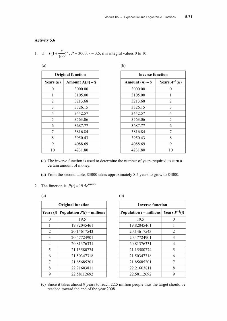
Module B5 – Exponential and Logarithmic Functions 5.71
Activity 5.6
1. , P = 3000, r = 3.5, n is integral values 0 to 10.
(c) The inverse function is used to determine the number of years required to earn a certain amount of money.
(d) From the second table, $3000 takes approximately 8.5 years to grow to $4000.
2. The function is
(c) Since it takes almost 9 years to reach 22.5 million people thus the target should be reached toward the end of the year 2008.
nrPA )
1001( %!
(a) (b)
Original function Inverse function
Years (n) Amount A(n) – $ Amount (n) – $ Years A–1(n)
0 3000.00 3000.00 0
1 3105.00 3105.00 1
2 3213.68 3213.68 2
3 3326.15 3326.15 3
4 3442.57 3442.57 4
5 3563.06 3563.06 5
6 3687.77 3687.77 6
7 3816.84 3816.84 7
8 3950.43 3950.43 8
9 4088.69 4088.69 9
10 4231.80 4231.80 10
tetP 0163.05.19)( !
(a) (b)
Original function Inverse function
Years (t) Population P(t) – millions Population t – millions Years P–1(t)
0 19.5 19.5 0
1 19.82045461 19.82045461 1
2 20.14617543 20.14617543 2
3 20.47724901 20.47724901 3
4 20.81376331 20.81376331 4
5 21.15580774 21.15580774 5
6 21.50347318 21.50347318 6
7 21.85685201 21.85685201 7
8 22.21603811 22.21603811 8
9 22.58112692 22.58112692 9
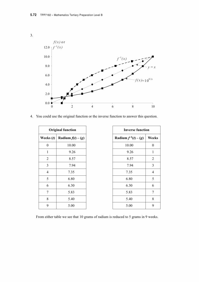
5.72 TPP7182 – Mathematics Tertiary Preparation Level B
3.
4. You could use the original function or the inverse function to answer this question.
From either table we see that 10 grams of radium is reduced to 5 grams in 9 weeks.
0.0
2.0
4.0
6.0
8.0
10.0
12.0
4 620 8 10
f ( x ) o r
y = x
f ( x )
( x )
( x )
f
f
=100.1x
-1
-1
Original function Inverse function
Weeks (t) Radium f(t) – (g) Radium f–1(t) – (g) Weeks
0 10.00 10.00 0
1 9.26 9.26 1
2 8.57 8.57 2
3 7.94 7.94 3
4 7.35 7.35 4
5 6.80 6.80 5
6 6.30 6.30 6
7 5.83 5.83 7
8 5.40 5.40 8
9 5.00 5.00 9
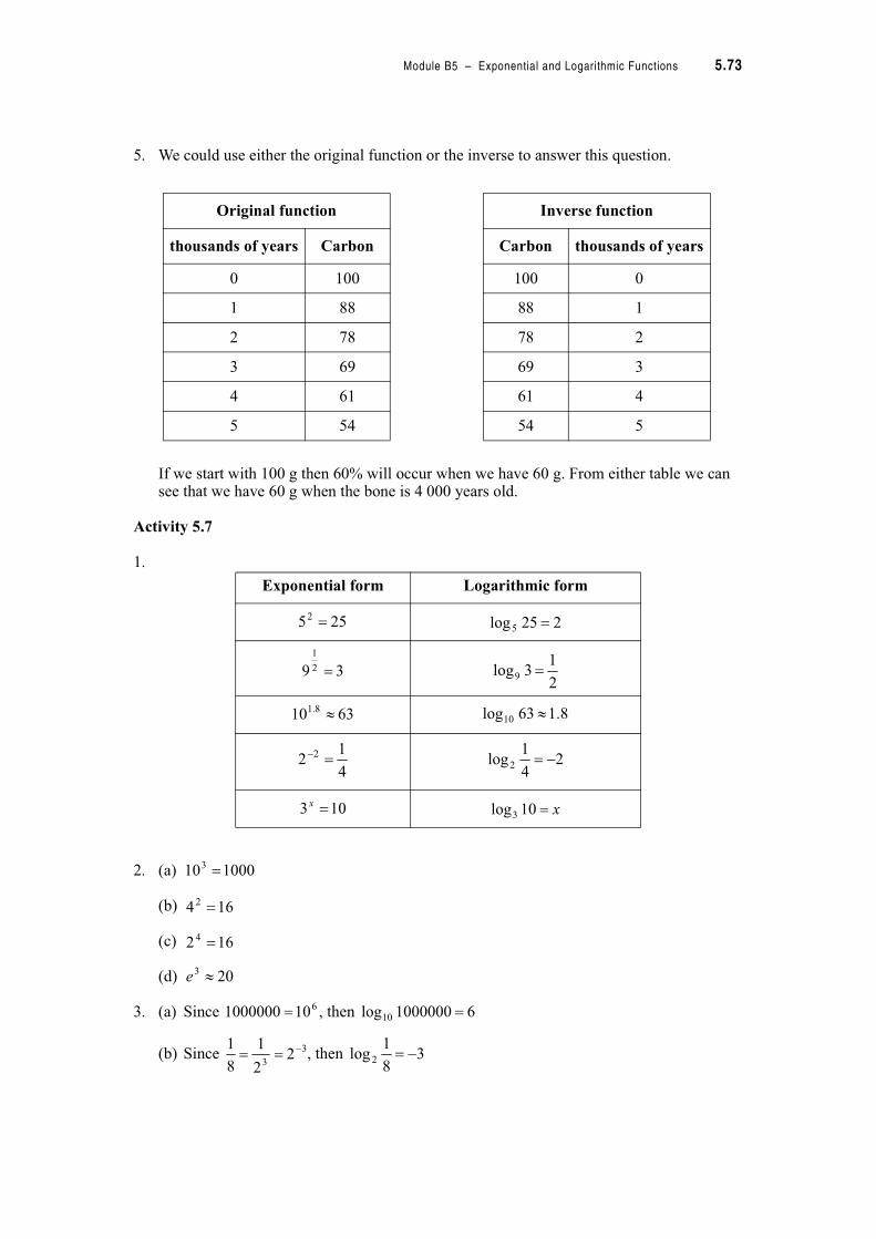
Module B5 – Exponential and Logarithmic Functions 5.73
5. We could use either the original function or the inverse to answer this question.
If we start with 100 g then 60% will occur when we have 60 g. From either table we can see that we have 60 g when the bone is 4 000 years old.
Activity 5.7
1.
2. (a)
(b)
(c)
(d)
3. (a) Since , then
(b) Since , then
Exponential form Logarithmic form
Original function Inverse function
thousands of years Carbon Carbon thousands of years
0 100 100 0
1 88 88 1
2 78 78 2
3 69 69 3
4 61 61 4
5 54 54 5
2552 ! 225log5 !
39 2
1
!2
13log9 !
6310 8.1 # 8.163log10 #
4
12 2
! 2
4
1log2 !
103 !xx!10log3
1000103 !
1642 !
1624 !
203 #e
6101000000 ! 61000000log10 !
3
32
2
1
8
1 !! 3
8
1log 2 !
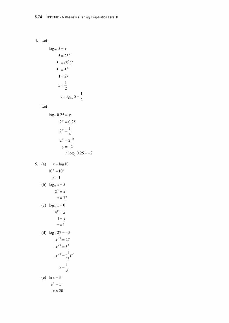
5.74 TPP7182 – Mathematics Tertiary Preparation Level B
4. Let
Let
5. (a)
(b)
(c)
(d)
(e)
2
15log
2
1
21
55
)5(5
255
5log
25
21
21
25
!'
!
!
!
!
!
!
x
x
x
x
x
x
225.0log
2
22
4
12
25.02
25.0log
2
2
2
!'
!
!
!
!
!
y
y
y
y
y
1
1010
10log
1
!
!
!
x
x
x
32
2
5log
5
2
!
!
!
x
x
x
1
1
4
0log
0
4
!
!
!
!
x
x
x
x
3
1
)3
1(
3
27
327log
33
33
3
!
!
!
!
!
x
x
x
x
x
20
3ln
3
#
!
!
x
xe
x
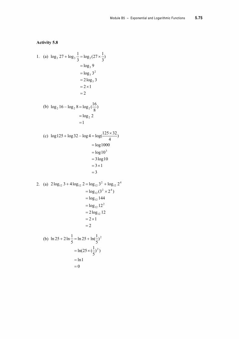
Module B5 – Exponential and Logarithmic Functions 5.75
Activity 5.8
1. (a)
(b)
(c)
2. (a)
(b)
2
12
3log2
3log
9log
)3
127(log
3
1log27log
3
23
3
333
!
"!
!
!
!
"!%
1
2log
)8
16(log8log16log
2
222
!
!
!
3
13
10log3
10log
1000log
)4
32125log(4log32log125log
3
!
"!
!
!
!
"! %
2
12
12log2
12log
144log
)23(log
2log3log2log43log2
12
212
12
4212
412
2121212
!
"!
!
!
!
"!
%!%
0
1ln
))5
1(25ln(
)5
1ln(25ln
5
1ln225ln
2
2
!
!
"!
%!%
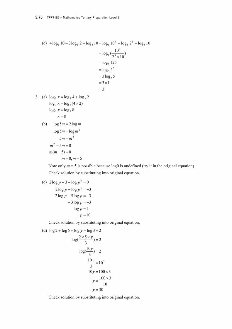
5.76 TPP7182 – Mathematics Tertiary Preparation Level B
(c)
3. (a)
(b)
Note only m = 5 is possible because log0 is undefined (try it in the original equation).
Check solution by substituting into original equation.
(c)
Check solution by substituting into original equation.
(d)
Check solution by substituting into original equation.
3
13
5log3
5log
125log
)102
10(log
10log2log10log10log2log310log4
5
35
5
3
4
5
53
54
5555
!
"!
!
!
!
"!
!
8
8loglog
)24(loglog
2log4loglog
33
33
333
!
!
"!
%!
x
x
x
x
5,0
0)5(
05
5
log5log
log25log
2
2
2
!!
!
!
!
!
!
mm
mm
mm
mm
mm
mm
10
1log
3log3
3log5log2
3loglog2
0log3log2
5
5
!
!
!
!
!
! %
p
p
p
pp
pp
pp
30
10
3100
310010
103
10
2)3
10log(
2)3
52log(
23loglog5log2log
2
!
"!
"!
!
!
!""
! %%
y
y
y
y
y
y
y
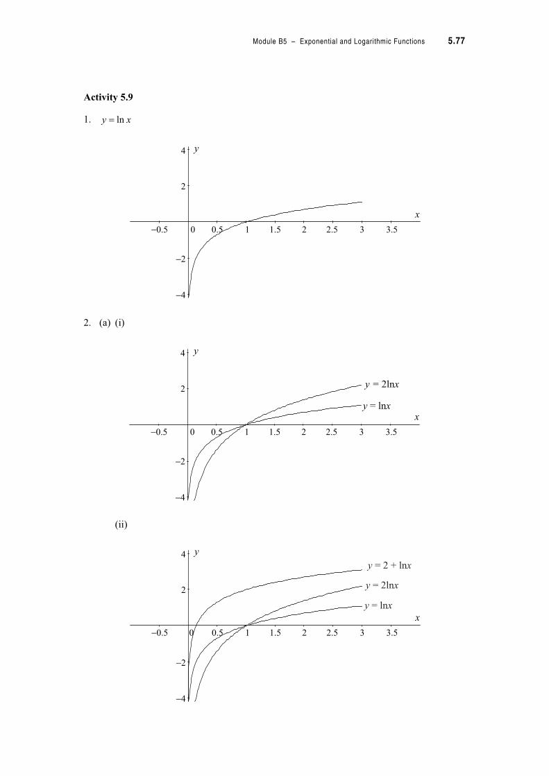
Module B5 – Exponential and Logarithmic Functions 5.77
Activity 5.9
1.
2. (a) (i)
(ii)
xy ln!
x
y
−0.5 0 0.5 1 1.5 2 2.5 3 3.5
−4
−2
2
4
x
y
−0.5 0 0.5 1 1.5 2 2.5 3 3.5
−4
−2
2
4
y = x2ln
y x= ln
x
y
−0.5 0 0.5 1 1.5 2 2.5 3 3.5
−4
−2
2
4
y x= 2 + ln
y x= 2ln
y x= ln
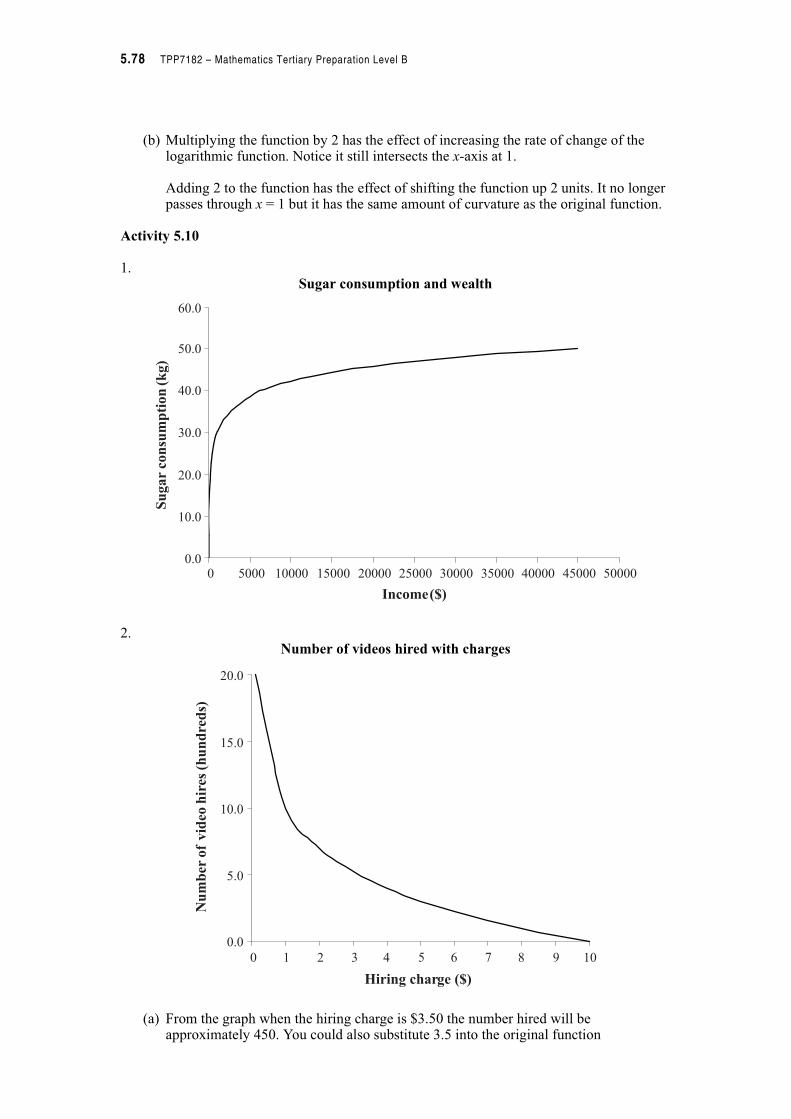
5.78 TPP7182 – Mathematics Tertiary Preparation Level B
(b) Multiplying the function by 2 has the effect of increasing the rate of change of the logarithmic function. Notice it still intersects the x-axis at 1.
Adding 2 to the function has the effect of shifting the function up 2 units. It no longer passes through x = 1 but it has the same amount of curvature as the original function.
Activity 5.10
1.Sugar consumption and wealth
2.Number of videos hired with charges
(a) From the graph when the hiring charge is $3.50 the number hired will be approximately 450. You could also substitute 3.5 into the original function
0 5000 10000 15000 20000 25000 30000 35000 40000 45000 500000.0
10.0
20.0
30.0
40.0
50.0
60.0
Sugar
consu
mption
(kg)
Income($)
0 1 2 3 4 5 6 7 8 9 10
0.0
5.0
10.0
15.0
20.0
Num
ber
of
vid
eohir
es(h
undre
ds)
Hiring charge ($)

Module B5 – Exponential and Logarithmic Functions 5.79
(b) Gross income from hires is number of videos multiplied by charge per video. If you compare the gross income for different numbers of videos:
$4 is the most profitable charge.
videos456
videosof hundreds 56.4
10
5.3log10
10log10
#
#
!
!
N
N
N
CN
Charge per video (C) Number hired (N) Gross income (C×N)
1 1000 1000
2 699 1398
3 523 1569
4 398 1592
5 301 1505
6 222 1332
7 155 1085
8 97 776
9 46 414
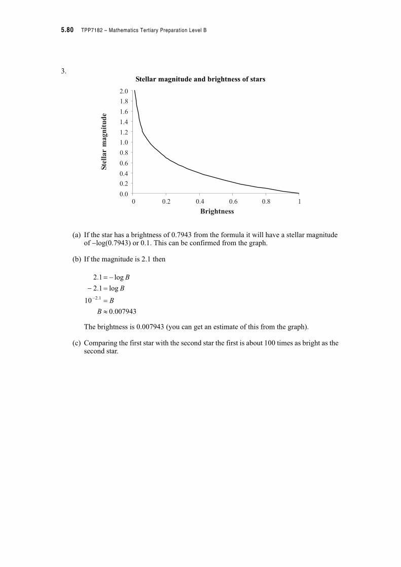
5.80 TPP7182 – Mathematics Tertiary Preparation Level B
3.Stellar magnitude and brightness of stars
(a) If the star has a brightness of 0.7943 from the formula it will have a stellar magnitude of log(0.7943) or 0.1. This can be confirmed from the graph.
(b) If the magnitude is 2.1 then
The brightness is 0.007943 (you can get an estimate of this from the graph).
(c) Comparing the first star with the second star the first is about 100 times as bright as the second star.
0 0.2 0.4 0.6 0.8 10.0
0.2
0.4
0.6
0.8
1.0
1.4
1.6
1.8
1.2
2.0
Ste
llar
magnitude
Brightness
007943.0
10
log1.2
log1.2
1.2
#
!
!
!
B
B
B
B
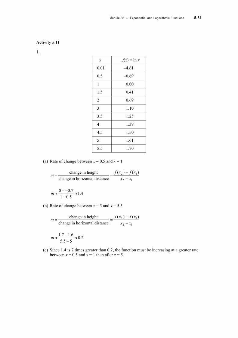
Module B5 – Exponential and Logarithmic Functions 5.81
Activity 5.11
1.
(a) Rate of change between x = 0.5 and x = 1
(b) Rate of change between x = 5 and x = 5.5
(c) Since 1.4 is 7 times greater than 0.2, the function must be increasing at a greater rate between x = 0.5 and x = 1 than after x = 5.
x f(x) = ln x
0.01 –4.61
0.5 –0.69
1 0.00
1.5 0.41
2 0.69
3 1.10
3.5 1.25
4 1.39
4.5 1.50
5 1.61
5.5 1.70
12
12 )()(
distance horizontalin change
heightin change
xx
xfxfm
!!
4.15.01
7.00#
#m
12
12 )()(
distance horizontalin change
heightin change
xx
xfxfm
!!
2.055.5
6.17.1#
#m
5.82 TPP7182 – Mathematics Tertiary Preparation Level B
2. (a) Rate of change between x = 2 500 and x = 5 000
(b) Rate of change between x = 12 500 and x = 15 000
(c) As the population size of a city increases the walking speed continues to increase but it is increasing at a reduced rate the large the population size by a factor of 6. (Note that this is just one way to describe the function…..you might have another way that is equally correct.)
(d) Although the function appears to work for the domain given I would imagine that there are finite limits to the speed of a person walking. The function could not increase indefinitely.
Activity 5.12
1. (a)
Note: You could have used log base e it makes no difference to the solution. Check your answer by substituting it back into the original equation.
(b)
Check your answer by substituting it back into the original equation.
12
12 )()(
distance horizontalin change
heightin change
xx
xfxfm
!!
00024.025005000
16.1#
#m
12
12 )()(
distance horizontalin change
heightin change
xx
xfxfm
!!
00004.01250015000
5.26.2#
#m
10
2log
1024log
1024log2log
1024log2log
10242
!
!
!
!
!
a
a
a
a
a
465.1
9log
25log
25log9log
25log9log
259
#
!
!
!
!
b
b
b
b
b
Module B5 – Exponential and Logarithmic Functions 5.83
(c)
Check your answer by substituting it back into the original equation.
(d)
Check your answer by substituting it back into the original equation.
(e)
Check your answer by substituting it back into the original equation.
768.0
27log
11log
7log
11log2
11log7log)2(
11log7log
117
2
2
#
!
!%
!%
!
!
%
%
c
c
c
c
c
c
209.0
5log
7log1
5log
7log1
7log5log)1(
7log5log
75
1
1
#
!
!
!
!
!
d
d
d
d
d
d
679.1
3log2
40log
3log
40log2
40log3log2
40log3log
403
2
2
#
!
!
!
!
!
x
x
x
x
x
x

5.84 TPP7182 – Mathematics Tertiary Preparation Level B
2. (a)
Check your answer by substituting it back into the original equation.
(b)
Check your answer by substituting it back into the original equation.(Note that this question could also be solved using the power rules from module 3.)
2
1
14log
8log
4log
8log1
8log4log)1(
8log4log
84
1
1
!
!
!%
!%
!
!
%
%
a
a
a
a
a
a
2
1
14log
8
1log
4log
8
1log
1
8
1log4log)1(
8
1log4log
8
14
1
1
!
%!
!
!
!
!
b
b
b
b
b
b
Module B5 – Exponential and Logarithmic Functions 5.85
(c)
Check your answer by substituting it back into the original equation.
(d)
Check your answer by substituting it back into the original equation.
(e)
Check your answer by substituting it back into the original equation.
Note all of the above questions could have just as easily been solved by taking log to the base e rather than log to the base 10 of both sides.
834.2
13log
2
15log
3log
2
15log
1
2
15log3log)1(
2
15log3log
2
153
1532
1
1
1
#
%!
!
!
!
!
!"
c
c
c
c
c
c
c
537.2
2444.3log
444.3log2
444.3log10log)2(
444.3log10log
444.310
444.2110
2
2
2
#
%!
!
!
!
!
!
d
d
d
d
d
d
d
Recall that log 10 = 1
151.2
3log5log
3log
3log)3log5(log
5log3log3log
5log3log)1(
5log3log
53
1
1
#
!
!
!%
!%
!
!
%
%
n
n
n
nn
nn
nn
nn
5.86 TPP7182 – Mathematics Tertiary Preparation Level B
3. (a)
(b)
(c)
a
bn
ban
ba
ba
n
n
log2
log
loglog2
loglog
2
2
22
22
!
!
!
!
4
ln
ln4
ln
ln4ln
lnln 4
4
4
4
a
y
n
e
a
y
n
ena
y
ea
y
ea
y
eay
aey
n
n
n
n
!
!
!
!
!
"!
!
Since we have e in the question we should take log base e.
)100
1log(
log
)100
1log(log
)100
1log(log
)100
1(
)100
1(
rP
A
n
rn
P
A
r
P
A
r
P
A
rPA
n
n
n
%
!
%!
%!
%!
%!
Module B5 – Exponential and Logarithmic Functions 5.87
(d)
(e)
(f)
)100
1log(
log
)100
1log(log
)100
1log(log
)100
1(
)100
1(
rP
D
n
rn
P
D
r
P
D
r
P
D
rPD
n
n
n
!
!
!
!
!
0166.0
)345.79
ln(
0166.0)345.79
ln(
ln0166.0)345.79
ln(
ln)345.79
ln(
345.79
345.79
345.79
0166.0
0166.0
0166.0
0166.0
!
!
!
!
!
"!
!
C
n
nC
enC
eC
eC
eC
eC
n
n
n
n
13ln
2lnln
3ln
)2
ln(
)3ln()2
ln(
)3ln()2
ln(
)3(2
)3(2
%
!
!
!
!
!
!
Ln
or
e
L
n
enL
eL
eL
eL
n
n
n
5.88 TPP7182 – Mathematics Tertiary Preparation Level B
Activity 5.13
1. , t = 0, A = 100
To find k use the values of t = 10 and A = 185
When t = 20
After 20 years the value is $342.12. ($342.25 if k is not rounded early in the process)
2. , when t = 0 and N = 100,
To find k use t = 2 and N = 60
ktPeA !
100
100 0
!
!
!
"
P
Pe
PeA
k
kt
0615.0
10
85.1ln
85.1ln10
ln1085.1ln
ln85.1ln
85.1
100185
10
10
10
#
!
!
!
!
!
"!
!
k
k
k
ek
e
e
e
PeA
k
k
k
kt
122.342
100 200615.0
!
!"
A
eA
kteNN ! 0
100
100
0
00
0
!
!
!
N
eN
eNN
k
kt
2554.0
2
60.0ln
ln260.0ln
ln60.0ln
60.0
10060
2
2
2
#
!
!
!
!
!
k
k
ek
e
e
e
k
k
k
Module B5 – Exponential and Logarithmic Functions 5.89
When N = 30
It takes approximately 4.7 years to reduce to 30 g.
3. , when t = 0 and T = 10 000, T0 = 10 000.
To find k, use t = 5 and T = 5000
When t = 10,
Temperature will be 2500$C in 10 million years.
4. , when t = 0, N = 2000, N0 = 2000
To find k use t = 2 and N = 2420
714.4
2554.0
30.0ln
ln2554.030.0ln
ln30.0ln
30.0
10030
2554.0
2554.0
2554.0
#
!
!
!
!
!
t
t
et
e
e
e
t
t
t
kteTT ! 0
1386.0
5
5.0ln
ln55.0ln
ln5.0ln
5.0
100005000
5
5
5
#
!
!
!
!
!
k
k
ek
e
e
e
k
k
k
2500
10000 101386.0
!
!"
T
eT
kteNN 0!
0953.0
2
21.1ln
ln221.1ln
ln21.1ln
21.1
20002420
2
2
2
#
!
!
!
!
!
k
k
ek
e
e
e
k
k
k
5.90 TPP7182 – Mathematics Tertiary Preparation Level B
When t = 24,
After 24 hours the numbers present are 19695.
5. , when t = 0 and P = 120 000, then P0 = 120 000.
To find k use t = 10 and P = 180 000
When P = 200 000
It will take approximately 12.6 years to reach 200 000.
65.19694
2000 240953.0
#
!"
N
eN
ktePP 0!
0405.0
10
5.1ln
ln105.1ln
ln5.1ln
5.1
120000180000
10
10
10
#
!
!
!
!
!
k
k
ek
e
e
e
k
k
k
6.12
0405.0
6666.1ln
ln0405.06666.1ln
ln6666.1ln
6666.1
120000200000
0405.0
0405.0
0405.0
#
#
#
#
#
!
t
t
et
e
e
e
t
t
t
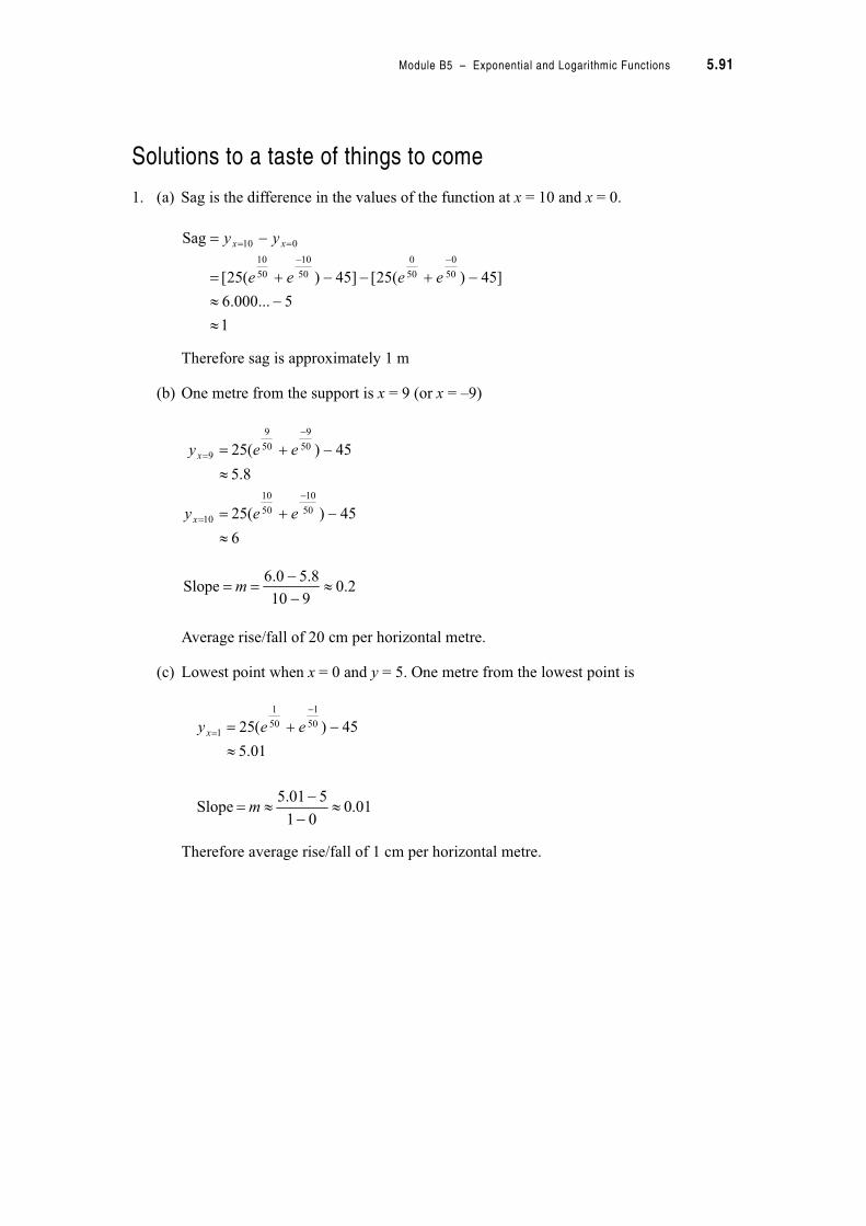
Module B5 – Exponential and Logarithmic Functions 5.91
Solutions to a taste of things to come
1. (a) Sag is the difference in the values of the function at x = 10 and x = 0.
Therefore sag is approximately 1 m
(b) One metre from the support is x = 9 (or x = –9)
Average rise/fall of 20 cm per horizontal metre.
(c) Lowest point when x = 0 and y = 5. One metre from the lowest point is
Therefore average rise/fall of 1 cm per horizontal metre.
1
5...000.6
]45)(25[]45)(25[
Sag
50
0
50
0
50
10
50
10
010
#
#
% %!
!
!!
eeee
yy xx
6
45)(25
8.5
45)(25
50
10
50
10
10
50
9
50
9
9
#
%!
#
%!
!
!
eey
eey
x
x
2.0910
8.50.6Slope #
!! m
01.5
45)(25 50
1
50
1
1
#
%!
! eey x
01.001
501.5Slope #
#! m
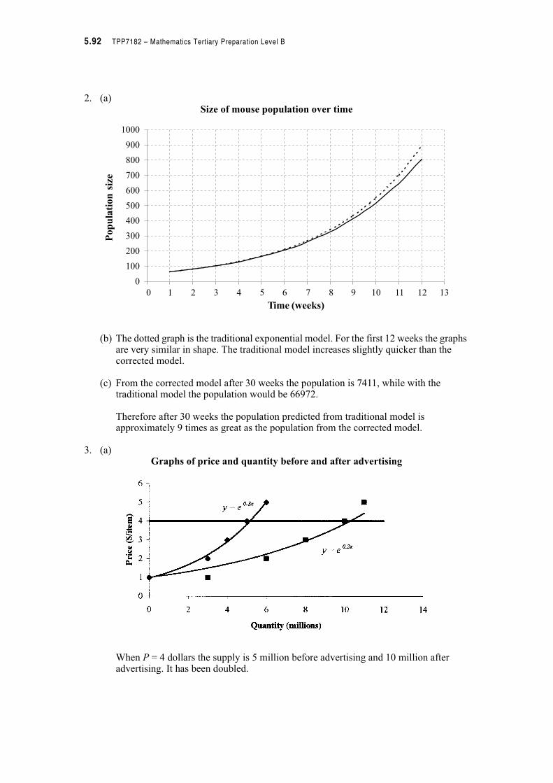
5.92 TPP7182 – Mathematics Tertiary Preparation Level B
2. (a)Size of mouse population over time
(b) The dotted graph is the traditional exponential model. For the first 12 weeks the graphs are very similar in shape. The traditional model increases slightly quicker than the corrected model.
(c) From the corrected model after 30 weeks the population is 7411, while with the traditional model the population would be 66972.
Therefore after 30 weeks the population predicted from traditional model is approximately 9 times as great as the population from the corrected model.
3. (a)Graphs of price and quantity before and after advertising
When P = 4 dollars the supply is 5 million before advertising and 10 million after advertising. It has been doubled.
0
0 1 2 3
Popula
tion
size
Time (weeks)
4 5 6 7 8 9 10 11 12 13
100
200
300
400
500
600
700
800
900
1000
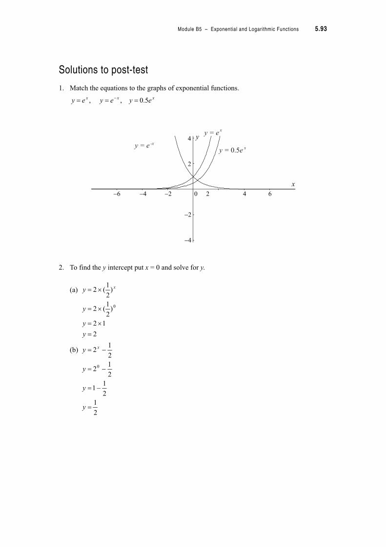
Module B5 – Exponential and Logarithmic Functions 5.93
Solutions to post-test
1. Match the equations to the graphs of exponential functions.
2. To find the y intercept put x = 0 and solve for y.
(a)
(b)
xxx eyeyey 5.0 , , !!!
x
y
−6 −4 −2 0 2 4 6
−4
−2
2
4y = e
y = e0.5
y = e
-x
x
x
2
12
)2
1(2
)2
1(2
0
!
"!
"!
"!
y
y
y
y x
2
1
2
11
2
12
2
12
0
!
!
!
!
y
y
y
y x
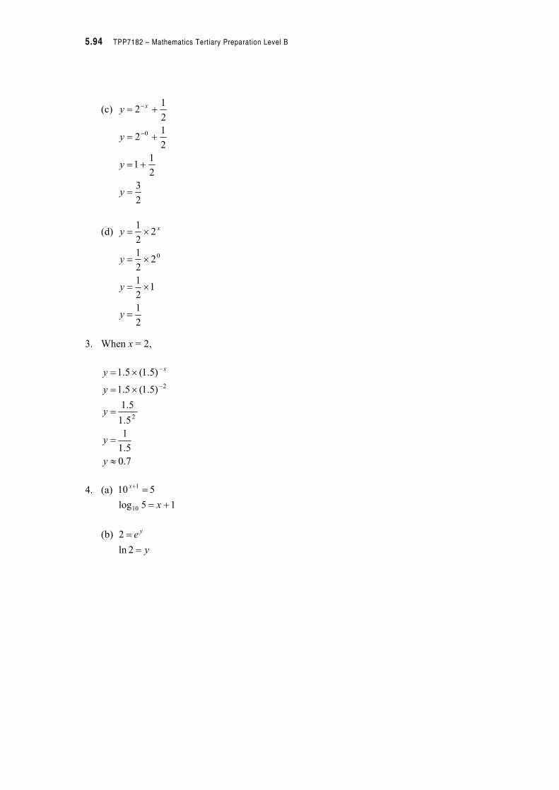
5.94 TPP7182 – Mathematics Tertiary Preparation Level B
(c)
(d)
3. When x = 2,
4. (a)
(b)
2
3
2
11
2
12
2
12
0
!
%!
%!
%!
y
y
y
y x
2
1
12
1
22
1
22
1
0
!
"!
"!
"!
y
y
y
y x
7.0
5.1
1
5.1
5.1
)5.1(5.1
)5.1(5.1
2
2
#
!
!
"!
"!
y
y
y
y
y x
15log
510
10
1
%!
!%
x
x
y
e y
!
!
2ln
2

Module B5 – Exponential and Logarithmic Functions 5.95
5. (a)
(b)
6. (a)
(b)
7. (a)
(b)
4
3log4
3log81log
3
433
!
!
!
3
)5
1(log3
)5
1(log
)5
1(log
)125
1(log125log
5
1
3
5
1
1
3
5
1
1
5
1
5
1
!
!
!
!
!
1.010
1.0log10
!
!
a
a
82
8log 2
!
!
b
b
4
5
2
2
22
5)2(log
!
!
!
p
p
p
15
10
10
405.010
ln
405.0
405.0
#
!
!
!
q
eq
qe
q
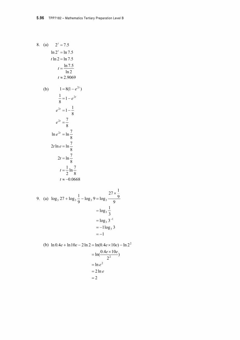
5.96 TPP7182 – Mathematics Tertiary Preparation Level B
8. (a)
(b)
9. (a)
(b)
9069.2
2ln
5.7ln
5.7ln2ln
5.7ln2ln
5.72
#
!
!
!
!
t
t
t
t
t
0668.0
8
7ln
2
1
8
7ln2
8
7lnln2
8
7lnln
8
7
8
11
18
1
)1(81
2
2
2
2
2
#
!
!
!
!
!
!
!
!
t
t
t
et
e
e
e
e
e
t
t
t
t
t
1
3log1
3log
3
1log
9
9
127
log9log9
1log27log
3
13
3
3333
!
!
!
!
"
! %
2
ln2
ln
)2
104.0ln(
2ln)104.0ln(2ln210ln4.0ln
2
2
2
!
!
!
"!
"! %
e
e
ee
eeee
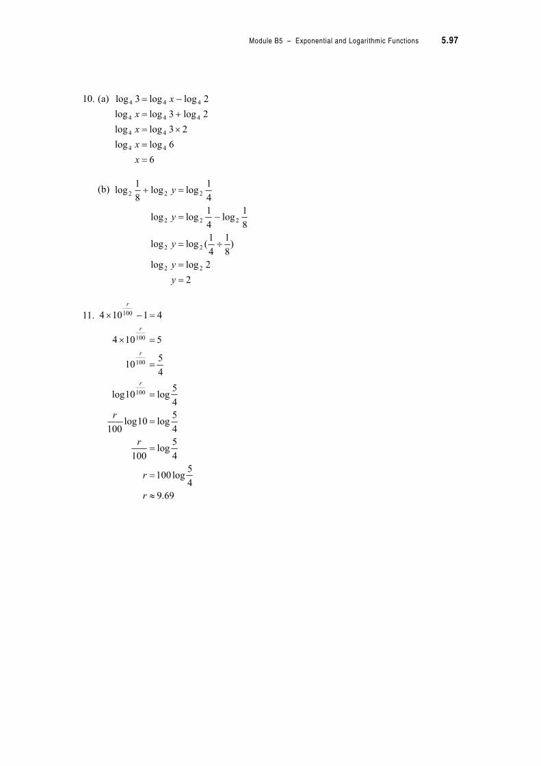
Module B5 – Exponential and Logarithmic Functions 5.97
10. (a)
(b)
11.
6
6loglog
23loglog
2log3loglog
2loglog3log
44
44
444
444
!
!
"!
%!
!
x
x
x
x
x
2
2loglog
)8
1
4
1(loglog
8
1log
4
1loglog
4
1loglog
8
1log
22
22
222
222
!
!
(!
!
!%
y
y
y
y
y
69.9
4
5log100
4
5log
100
4
5log10log
100
4
5log10log
4
510
5104
41104
100
100
100
100
#
!
!
!
!
!
!"
! "
r
r
r
r
r
r
r
r
5.98 TPP7182 – Mathematics Tertiary Preparation Level B
12.
13. Given the original equation we can rearrange it to become the second expression.
Thus the first equation is equivalent to the second equation.
14.
6.0
)4.1
3ln(
6.04.1
3ln
ln6.04.1
3ln
ln4.1
3ln
4.1
3
4.13
34.1
6.0
6.0
6.0
6.0
%
!
!%
!%
!%
!%
!%
!
y
t
ty
ety
ey
ey
ey
ey
t
t
t
t
1ln
3lnln
lnln
3lnln
)ln(
3ln
)ln(3
ln
)ln(3
ln
)(3
)(3
%
!
%
!
!
!
!
!
"!
a
gn
ea
gn
ae
g
n
aeng
aeg
aeg
aeg
n
n
n
)1ln(
ln
)1ln(ln
)1ln(ln
)1(
)1(
i
P
A
n
inP
A
iP
A
iP
A
iPA
n
n
n
%!
%!
%!
%!
%!
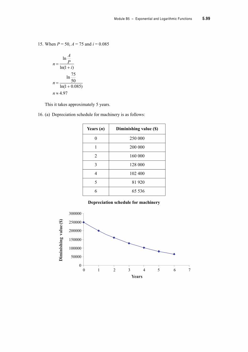
Module B5 – Exponential and Logarithmic Functions 5.99
15. When P = 50, A = 75 and i = 0.085
This it takes approximately 5 years.
16. (a) Depreciation schedule for machinery is as follows:
Depreciation schedule for machinery
Years (n) Diminishing value ($)
0 250 000
1 200 000
2 160 000
3 128 000
4 102 400
5 81 920
6 65 536
97.4
)085.01ln(
50
75ln
)1ln(
ln
#
%!
%!
n
n
i
P
A
n
00 21 3 4 5 6 7
50000
100000
150000
200000
250000
300000
Years
Dim
inis
hin
gvalu
e($
)
5.100 TPP7182 – Mathematics Tertiary Preparation Level B
(b)
(c) If n = 10
Depreciated value is approximately $26844.
17. When t = 5
Voltage is approximately 1.889 volts.
18.
(a) Present value occurs when t = 0,
Value is 12 g
(b) Half of the original mass is 6 g.
It takes approximately nine and a quarter years to reach its half-life.
n
n
n
nD
nD
rPnD
)8.0(250000)(
)100
201(250000)(
)100
1()(
"!
!
!
55.26843
)8.0(250000)( 10
#
"!nD
889.1
....88875.1
10
10
3
5
3
#
!
!
!
V
V
eV
eV
t
teR 075.012 !
12
12 0075.0
!
!"
R
eR
24.9
075.0
5.0ln
075.05.0ln
ln075.05.0ln
ln5.0ln
5.0
126
12
075.0
075.0
075.0
075.0
#
!
!
!
!
!
!
!
t
t
t
et
e
e
e
eR
t
t
t
t

Module B5 – Exponential and Logarithmic Functions 5.101
19.
Find P for the years 1981, 1986, 2001 and 2006 using the above formula.
Rate of growth (1981 to 1986),
Rate of growth (2001 to 2006),
If we compare growth rates we find that 0.088 is one and one third times the value of 0.066. Thus population is predicted to grow faster in the next century.
20.
When n = 60
When n = 50
When n = 40
Year Time (years –t) Population (billions –P)
1981 0 4.5
1986 5 4.83
2001 20 5.98
2006 25 6.42
teP 0142.05.4!
yearper billion 066.0
05
5.483.41
#
#m
yearper billion 088.0
2025
98.542.62
#
#m
nP 1.01020"!
P 1020
1020
1020
6
601.0
1.0
&"!
"!
"!
"
P
P
P n
P 1020
1020
1020
5
501.0
1.0
&"!
"!
"!
"
P
P
P n
P 1020
1020
1020
4
401.0
1.0
&"!
"!
"!
"
P
P
P n
5.102 TPP7182 – Mathematics Tertiary Preparation Level B
Comparing 60 decibels with 50 decibels we find that the loudness 60 decibels is 10 times
that of 50 decibels because .
Comparing 60 decibels with 40 decibels we find that the loudness 60 decibels is 100 times
that of 40 decibels because .
10P 1020
P 10205
6
!"
"
&
&
100P 1020
P 10204
6
!"
"
&
&