module c-cs: calculations for estimating carbon stocks · leaf technical guidance series for the...

LEAF TECHNICAL GUIDANCE SERIES FOR THE DEVELOPMENT OF A FOREST CARBON

MONITORING SYSTEM FOR REDD+

Module C-CS: Calculations for Estimating Carbon Stocks

Katherine Goslee, Sarah M Walker, Alex Grais, Lara Murray, Felipe Casarim, and Sandra Brown

LEAF TECHNICAL GUIDANCE SERIES FOR THE DEVELOPMENT OF A FOREST CARBON MONITORING SYSTEM FOR REDD+

Module C-CS: Calculations for Estimating Carbon Stocks Katherine Goslee, Sarah M Walker, Alex Grais, Lara Murray, Felipe Casarim, and Sandra Brown

Winrock International

TABLE OF CONTENTS 1. Scope ......................................................................................................................................... 2 2. Applicability ............................................................................................................................... 2 3. Products ..................................................................................................................................... 2 4. Required Inputs .......................................................................................................................... 2 5. Methods and Procedures ............................................................................................................ 3

Statistical Measures ...................................................................................................................................3 Plot Analysis.......................................................................................................................................6 Calculation of Sampled Plot Area ......................................................................................................6 Calculation of Scaling Factors ......................................................................................................... 11

Calculating Carbon Stocks in each Carbon Pool ...................................................................................... 12 Calculation of Live Tree Carbon Stocks .......................................................................................... 12 Calculations for Cluster Plots .......................................................................................................... 15 Calculation of Density from Wood Samples ................................................................................... 17 Calculation of Standing Dead Wood Carbon Stocks ....................................................................... 18 Calculation of Lying Dead Wood Carbon Stocks ............................................................................ 21 Calculation of Carbon Stocks from Clip Plots ................................................................................. 23 Calculation of Carbon Stocks from Saplings ................................................................................... 26 Calculation of Soil Carbon Stocks ................................................................................................... 29 Wood Products ............................................................................................................................... 31

Total Biomass Carbon Stocks and Propagation Uncertainty ................................................................... 32 Calculating Total Carbon Stocks ..................................................................................................... 32 Uncertainty Propagation ................................................................................................................ 33

Other Calculations ................................................................................................................................... 36 Tree Biomass from Destructive Sampling ...................................................................................... 36 Incremental Change in Tree Carbon Stocks Over Time .................................................................. 39

LEAF REDD+ Technical Guidance Series |Module C-CS 2

1. SCOPE This module describes the calculations necessary to estimate carbon stocks and their uncertainty, based on field data collected in a Terrestrial Carbon Monitoring System for REDD+.

The following guidance provide the steps needed to convert field measurements into mean carbon stock estimates for various pools and for estimating net change in carbon stocks. Guidance is provided on calculation of the following components of data analysis:

• Statistical Measures • Plot Analysis

o Plot Area Calculation o Scaling Factor

• Carbon Stocks o Live Tree (including calculations for cluster sampling) o Standing Dead Wood o Lying Dead Wood o Clip Plots (litter and herbaceous vegetation) o Saplings o Soil

• Wood Products • Total stocks & total uncertainty • Destructive Sampling • Change in tree carbon stocks over time

2. APPLICABILITY The module is applicable for calculating carbon stocks using field data collected in accordance with Standard Operating Procedures developed using Walker et al, 20121.

3. PRODUCTS This module provides the methods and procedures to calculate forest carbon stocks and their uncertainty for all potential carbon pools.

4. REQUIRED INPUTS In general, required input includes all field data, plot size(s), necessary allometric equations and/or ratios, and uncertainty requirements. Each section on individual calculations includes a specific list of required inputs to conduct those calculations. 1 Walker, SM, TRH Pearson, FM Casarim, N Harris, S Petrova, A Grais, E Swails, M Netzer, KM Goslee and S Brown. 2012. Standard Operating Procedures for Terrestrial Carbon Measurement: Version 2012. Winrock International.


5. METHODS AND PROCEDURES

Statistical Measures

Estimation of carbon stocks is based on sampling a population of interest, for example one forest stratum, rather than taking measurements of the entire population. The purpose of sampling is to achieve a representative data set of the population in as efficient a manner as possible. Data collected through sampling can be used to infer information about the population through a set of descriptive statistics, which typically includes a measure of central tendency and an estimate of the variability of this measure. Below some basic standard statistical equations are provided.

The arithmetic mean (mean) is the average value of the sampled observations and provides a measure of central tendency.

�̅� =1𝑛�𝑥𝑖

𝑛

𝑖

(1)

Where: x = mean

x = sampled value n = number of samples i = 1,…., n

The standard deviation provides a measurement of variation from the average value, and is calculated as the square root of the variance.

𝑠 = �1

𝑛 − 1�(𝑥𝑖 − �̅�)2𝑛

𝑖

(2) Where:

s = sample standard deviation x = sampled value n = number of samples i = 1,….,n x = mean

The standard error provides the standard deviation of the mean and is estimated by dividing the standard deviation by the square root of the number of observations.

𝑆𝐸�̅� =𝑠√𝑛


(3)

Where:

SE = standard error x = mean s = sample standard deviation n = number of samples

The confidence interval gives the estimated range of values likely to include an unknown population parameter at the chosen confidence level.

𝐶𝐼 = 𝑡 ∗ 𝑆𝐸�̅�

(4)

Where:

CI = confidence interval at a specific confidence level, often 95% t = t-value, a function of the confidence level and n. This can be found using a

look-up table or calculated in excel using the function TINV2.

SE = standard error

x = mean

The resulting range is then generally expressed as the mean plus or minus the confidence interval (�̅�±CI).

Uncertainty is a key metric to portray the confidence in calculations and an uncertainty assessment quantifies the variability of estimates, based on accuracy and/or precision of measurements3. Such an assessment is required for REDD+ accounting under IPCC, UNFCCC, and all major greenhouse gas standards and registries. Uncertainty is estimated for individual measurements such as biomass in carbon pools as well as aggregations of measurements such as the sum of carbon across pools and the development of emission factors. There are many ways to express uncertainty, but it is commonly represented as a percentage, and often there is an acceptable level of uncertainty defined.

Uncertainty can be expressed using the confidence interval as a percent of the mean.

𝑈𝑛𝑐𝑒𝑟𝑡𝑎𝑖𝑛𝑡𝑦 =𝐶𝐼�̅�

(5)

Where:

CI = confidence interval at a specific confidence level, often 95%

2 For example, for a 95% confidence interval and a sample size of 20, the correct syntax is “=TINV(0.05,19)”. Nineteen represents n-1, or 20-1 in this case. 3 Uncertainty can result from factors such as bias or inaccurate definitions that cannot be addressed by statistical means. Such uncertainties must instead be identified and reduced to the extent possible.


x = mean

During field sampling, a certain precision and uncertainty is usually targeted. In some instances, estimates may be required to achieve a specified target. A common uncertainty target is less than 15% of the mean at a 95% confidence interval. If a lower confidence interval is used, the percent of the mean must be lower as well, such as 10% of the mean at a 90% confidence interval. If the data set does not achieve the desired level of uncertainty, additional measurements must be collected to reduce uncertainty. This will be described in more detail in the module on sample design.

Methods for aggregating uncertainties across measurements are described in a later section.


Plot Analysis

Calculation of Sampled Plot Area

Plots or nested plots are assumed to be circular, with the basic area calculated as the area of a circle:

𝐴 = 𝜋𝑅2

Where: A = Area of nest R = Radius of nest

However, all data on carbon stocks of pools are expressed on the horizontal projection of a unit area of land. Where plots are on sloped ground, an adjustment must be made either during fieldwork or data analysis so that the plot area reflects the true horizontal projection. The calculations required for each of these adjustments are described below.

The SOP field manual used to conduct field measurements should be consulted to determine which option was used in the field, and therefore, which calculation option should be used.

Generally, if the slope is less than a certain value, usually 10% (5.74 degrees), the impact of the slope on distorting the true horizontal projection is insignificant and ignored. The SOP field manual used to conduct field measurements should be consulted to determine what threshold was used for adjustment. In cases where the threshold is not met (e.g. the slope is less than 10%), the length measured in the field is assumed to equal the true horizontal length and no correction is conducted.

Option 1: Adjustment during fieldwork

Under this option, the horizontal projection of the nest area is kept constant for all plots in a stratum, and instead the on-the-ground nest size is adjusted in the field to account for the slope. To adjust the nest size, the radius of the circular nest is changed.

Calculations completed while in field:

This is done through a three part process.

In the first step, it is imagined that the horizontal area of the nest is projected onto the sloped ground. Since the land is on a slope, such a projection will create an ellipse. A calculation is made to determine what the radius that lies along the slope would be:

𝑁𝑅𝑠𝑙𝑜𝑝𝑒𝑑 =𝑁𝑅𝐶𝑜𝑠 𝜃

(6)

Where: NRsloped = Length of nest radius (m) on slope that corresponds to horizontal radius NR = Length of nest radius agreed upon in flat terrain (m) Cos θ = Cosine of the slope angle, in degrees

In the second step, the area of such an ellipse is then calculated:

𝑵𝑨𝒆𝒍𝒍𝒊𝒑𝒔𝒆 = 𝝅 ∗ 𝑵𝑹 ∗ 𝑵𝑹𝒔𝒍𝒐𝒑𝒆𝒅


(7)

Where: NAellipse = Ellipse nest area (m2) NR = Original length of nest radii (m) (radii parallel to horizontal projection) NRsloped = Length of nest radii (m) lying along the slope

However, it is extremely difficult to accurately measure an ellipse in the field. Instead, in the third step entails calculating the radius of a circle with an area equivalent to the area of the ellipse. The radius corrected for slope, to be used in the field, is then calculated as follows:

𝑵𝑨𝒄𝒐𝒓𝒓𝒆𝒄𝒕𝒆𝒅 = 𝑵𝑨𝒆𝒍𝒍𝒊𝒑𝒔𝒆 (8)

𝑵𝑹𝒄𝒐𝒓𝒓𝒆𝒄𝒕𝒆𝒅 = �𝑵𝑨𝒄𝒐𝒓𝒓𝒆𝒄𝒕𝒆𝒅𝝅

(9)

Where: NAellipse = Ellipse nest area (m2) NRcorrected = Corrected length of nest radius (m) NAcorrected =Corrected nest area (m2)

This correction must be repeated for each nest size in the plot. However, instead of actually performing the above calculations in the field, it is recommended that a correction look-up table be used and this table should be included within the SOP manual used. This table will provide a list of nest sizes, slopes, and resulting corrected nest radius to be used in the field.

Calculation completed during data analysis:

During data analysis the circular nest area in the plot shall then be calculated as follows:

𝑁𝐴 = 𝜋 ∗ 𝑁𝑅𝑐𝑜𝑟𝑟𝑒𝑐𝑡𝑒𝑑2 (10)

Where: NA = Horizontally projected area of a circular nested plot (m2) NRcorrected = Corrected length of nest radius (m)

This correction should be repeated for each nest size in the plot.

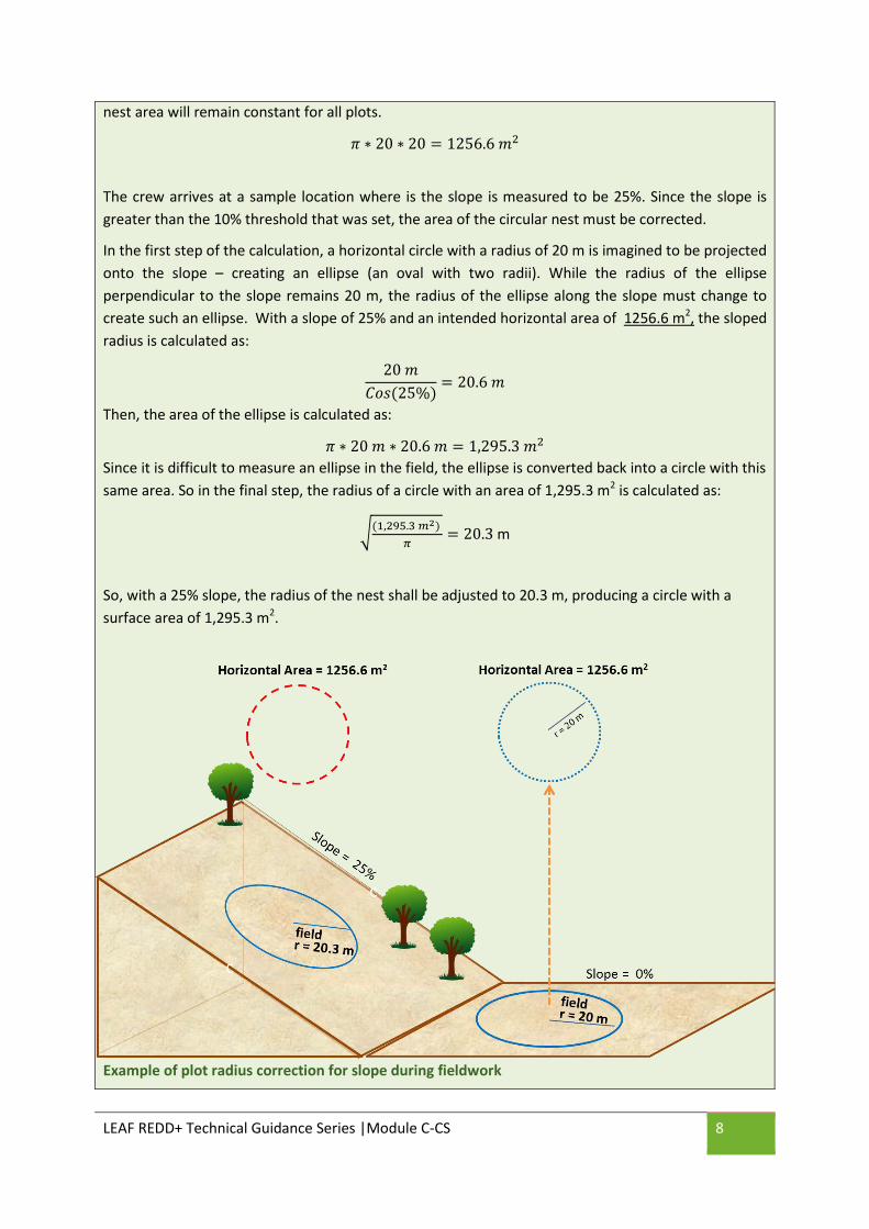
Example of plot size adjustment due to slope completed during fieldwork:

In this example, based on the type of forest to be sampled, it has been decided that on a flat terrain, the plot radius of the largest nest will be 20m. Therefore, the plot area is 1256.6 m2. This horizontal


nest area will remain constant for all plots.

𝜋 ∗ 20 ∗ 20 = 1256.6 𝑚2

The crew arrives at a sample location where is the slope is measured to be 25%. Since the slope is greater than the 10% threshold that was set, the area of the circular nest must be corrected.

In the first step of the calculation, a horizontal circle with a radius of 20 m is imagined to be projected onto the slope – creating an ellipse (an oval with two radii). While the radius of the ellipse perpendicular to the slope remains 20 m, the radius of the ellipse along the slope must change to create such an ellipse. With a slope of 25% and an intended horizontal area of 1256.6 m2, the sloped radius is calculated as:

20 𝑚𝐶𝑜𝑠(25%)

= 20.6 𝑚

Then, the area of the ellipse is calculated as:

𝜋 ∗ 20 𝑚 ∗ 20.6 𝑚 = 1,295.3 𝑚2 Since it is difficult to measure an ellipse in the field, the ellipse is converted back into a circle with this same area. So in the final step, the radius of a circle with an area of 1,295.3 m2 is calculated as:

�(1,295.3 𝑚2) 𝜋

= 20.3 m

So, with a 25% slope, the radius of the nest shall be adjusted to 20.3 m, producing a circle with a surface area of 1,295.3 m2.

Example of plot radius correction for slope during fieldwork


Option 2: Adjustment during data analysis

When adjustments are to be made during data analysis, there is no need to adjust nest sizes during field measurements. Instead, the slope is recorded for each plot in the field. Adjustment calculations are then applied during data analysis.

This option allows nests on sloped surfaces to be measured using the same radius for all plots, regardless of the slope. Then, during data analysis, the area of the plot is corrected to reflect the fact that the nest’s horizontal projection creates an ellipse. As ellipses have two radii, it is assumed the first radius of the ellipse is parallel with the horizon while the other is parallel to the slope in the field. Therefore, a calculation is conducted to estimate the horizontal projection of the radii lying along the slope:

𝑅𝑠𝑙𝑜𝑝𝑒−ℎ𝑜𝑟𝑖𝑧𝑜𝑛𝑡𝑎𝑙 = 𝑅𝑓𝑖𝑒𝑙𝑑 ∗ cos𝜃 (11)

Where:

Rslope-horizontal = Projected horizontal length of the radii lying parallel to the slope in the nest (m) Rfield = Radius of nest measured in the field (m) cos θ = Cosine of the slope, in degrees; slope in degrees = arctangent (% slope)4

The area of this horizontal ellipse is then calculated using these two radii:

𝑁𝐴 = 𝜋 ∗ 𝑅 𝑓𝑖𝑒𝑙𝑑 ∗ 𝑅𝑠𝑙𝑜𝑝𝑒−ℎ𝑜𝑟𝑖𝑧𝑜𝑛𝑡𝑎𝑙 (12)

Where:

NA = Horizontally projected area of a circular nested plot (m2) Rfield =Radius of the nest, measured in the field (m) Rslope-horizontal = Projected horizontal length of the radii lying parallel to the slope in the nest (m)

This correction should be repeated for each nest size in the plot.

4 Note that when conducting calculations using Excel, percent slope is converted to degrees using the following functions: =ATAN(DEGREES(% slope)).


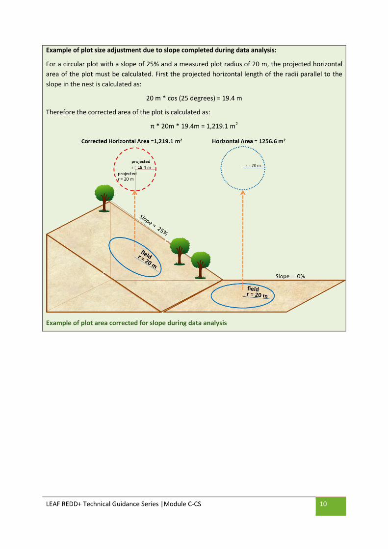
Example of plot size adjustment due to slope completed during data analysis:

For a circular plot with a slope of 25% and a measured plot radius of 20 m, the projected horizontal area of the plot must be calculated. First the projected horizontal length of the radii parallel to the slope in the nest is calculated as:

20 m * cos (25 degrees) = 19.4 m

Therefore the corrected area of the plot is calculated as:

π * 20m * 19.4m = 1,219.1 m2

Example of plot area corrected for slope during data analysis


Calculation of Scaling Factors

When field measurements are taken within plots, a known measured area is sampled. A scaling factor is then used to extrapolate the field measurements taken (e.g. mass of AG tree carbon within sampled plot) to a ‘per hectare’ basis. This scaling factor is converting the area units from square meters to one hectare:

𝑆𝐹 =10,000𝑁𝐴

(13)

Where: SF = scaling factor to convert to per hectare basis (dimensionless)

10,000 = meters squared in one hectare NA = horizontally projected area of nested plot (m2)

When nested subplots5 are used, a unique scaling factor should be developed for each nest.

Scaling Factor Example: A plot with a series of nested circular plots measuring 4 m, 14 m and 20 m in radius, uses the following scaling factors:

Plot radius (m) Horizontal plot radius (m)

Plot Area (m2) Scaling Factor

4 4 50 198.94 14 14 616 16.24 20 20 1,257 7.96

In other words, a 4-meter radius plot on relatively flat land represents 198.94 plots per hectare, a 14-meter radius represents 16.24 plots per acre, and a 20-meter radius plot represents 7.96 plots per hectare.

5 For information on nested plots see: Walker, SM, TRH Pearson, FM Casarim, N Harris, S Petrova, A Grais, E Swails, M Netzer, KM Goslee and S Brown. 2012. Standard Operating Procedures for Terrestrial Carbon Measurement: Version 2012. Winrock International.


Calculating Carbon Stocks in each Carbon Pool

Calculation of Live Tree Carbon Stocks

To estimate the stocks of live tree carbon in the area of interest, the biomass of all sampled trees is first estimated and then a plot-level estimate is calculated. A mean carbon stock is then calculated by taking the average of all plot estimates.

One or more allometric equations are used to estimate the live aboveground biomass of the sampled trees. (See the SOPs for more information on identifying and developing allometric equations.) The biomass estimate is converted to tons of carbon and the scaling factor is applied to estimate carbon stocks on a per hectare basis. The biomass of all trees sampled in each plot is then summed to estimate a total carbon stock in each sampled plot. Unlike aboveground biomass, allometric equations for belowground biomass based on metrics such as DBH do not generally exist. However, belowground biomass for forests is highly correlated with estimates of aboveground biomass. A synthesis of global data by Mokany et al6, and used in the IPCC 2006 guidelines, provides simple equations that estimate belowground biomass based on aboveground biomass or based on a series of root-to-shoot (R/S) ratios by major forest types.

Information required to complete the analysis:

• Field data • Scaling factor(s), for all relevant plot and/or nest sizes • Allometric equation(s) to be applied to all tree species sampled • Any additional parameters required to complete allometric equation (for example, wood

density) • Belowground biomass equation or ratio

Calculation Steps:

1. If adjustment for slope is made during data analysis, ensure the horizontal area and the scaling factor have been calculated for each plot or subplot. (If adjustment for slope is made during the fieldwork, this step is not necessary.)

2. For each tree in the plot, calculate AG biomass using the selected allometric equation(s) and weight of average sapling.

3. To estimate the biomass of each tree on a per hectare basis multiply the tree biomass by the correct scaling factor based on the size of the plot or nest in which the tree was measured.

4. Convert biomass in kilograms to biomass in tons, if applicable. The units of biomass used in allometric equations are often kg dry biomass, in which case conversion to tons requires multiplying by 0.001.

5. Sum the biomass per hectare of all trees across all nests in each plot.

6 Mokany, K., R.J. Raison, A.S. Prokushkin. 2006. Critical analysis of root: shoot ratios in terrestrial biomes. Global Change Biology 11:1-3.


6. Apply appropriate equation or R/S ratio for calculation of BG biomass for each plot7. 7. Convert estimates of biomass to carbon:

𝐶𝑝 = 𝐷𝑀 ∗ 𝐶𝐹

(14)

Where:

Cp = carbon stock in plot (t C ha-1) DM = dry biomass in plot (t dry matter ha-1)

CF = carbon fraction (t C t-1 dry matter). For tree vegetation, use the Carbon Fraction 0.47 t C t-1 dry matter or species-specific values from the literature (per IPCC 2006 GL, V4, Ch4, Table 4.38).

8. Calculate the mean and confidence interval AG and BG carbon pools for the stratum.

7 Root-to-shoot ratios to calculate belowground biomass are generally based on aboveground biomass for an entire plot, rather than an individual tree. 8 http://www.ipcc-nggip.iges.or.jp/public/2006gl/pdf/4_Volume4/V4_04_Ch4_Forest_Land.pdf


Live Tree Carbon Stock Calculation Example: The table below shows hypothetical data and biomass and carbon calculations for one nested plot. The tree size distributions measured within each nest are as follows: 5-20 dbh in 4m radius nest; 20-50 in 14m radius nest; >50 dbh in 20 m radius nest. Aboveground biomass is calculated based on an equation from Chave et al*:

AGB = Wood Density (g/cm3)*EXP(-1.499+(2.148*LN(DBH))+(0.207*(LN(DBH))2) -(0.0281*(LN(DBH))3))

Wood Density is assumed to be 0.6 g/cm3 for all trees. Belowground biomass was calculated following Mokany et al¥:

BGB = AGB(tC/ha) * 0.235

Plot # Tree#

DBH (cm)

Nest Biomass (kg)

Scaling factor

Biomass (kg/ha)

1 001 16.3 Small 146.53 198.94 29,150.96

1 002 18.7 Small 210.64 198.94 41,906.48

1 003 48.1 Medium 2,398.56 16.24 38,953.31

1 004 8.9 Small 29.41 198.94 5,851.75

1 005 9.2 Small 32.12 198.94 6,389.30

1 006 62.8 Large 4,613.60 7.96 36,713.90

1 007 26.4 Medium 519.97 16.24 8,444.49

1 008 23.0 Medium 362.89 16.24 5,893.37

1 009 55.0 Large 3,340.15 7.96 26,580.09

1 010 5.3 Small 7.52 198.94 1,496.39

Aboveground Live Tree Biomass (kg/ha) 201,380.04

Aboveground Live Tree Carbon (tC/ha) 94.65

Belowground Live Tree Carbon (tC/ha) 22.24

Total Live Tree Carbon (tC/ha) 116.89

* Chave, J., C. Andalo, S. Brown, M.A. Cairns, J.Q. Chambers, D. Eamus, H. Folster, F. Fromard, N. Higuchi, T. Kira, J.-P. Lescure, B.W. Nelson, H. Ogawa, H. Puig, B. Riera, and T. Yamakura. 2005. Tree allometry and improved estimation of carbon stocks and balance in tropical forests. Oecologia 145:87-99. ¥ Mokany, K., R.J. Raison, A.S. Prokushkin. 2006. Critical analysis of root: shoot ratios in terrestrial biomes. Global Change Biology 11:1-3.


Calculations for Cluster Plots

The calculations when using cluster plots can be completed using two methods.

Simplified Cluster Analysis Method

This first method is simpler. Under this method, the average of all subplots in a cluster is calculated and this value can be used as a plot-level estimate. This provides a simple method of estimating uncertainty. This method accounts for only the inter-cluster (between clusters) variance and not the intra-cluster (within clusters) variance.

1. Calculate the carbon stocks of each subplot in a cluster 2. Calculate the average carbon stock of all subplots in cluster 3. Calculate the standard deviation, standard error, and uncertainty across clusters (n = number

of clusters)

Comprehensive Cluster Analysis Method

In this method, both the inter-cluster and the intra-cluster variance are used to calculate the total variance. Including intra-cluster variance requires use of the following calculations, where:

All clusters have the same number of subplots n = number of clusters m = number of subplots in each cluster xij = mean value of the subplot j in cluster i

�̅�𝑖 = mean value of cluster i

The population mean (µ) is the overall mean as described above, estimated as:

𝜇 =1𝑛��

1𝑚�𝑥𝑖𝑗𝑗

�𝑗

=1𝑛𝑚

�𝑥𝑖𝑗𝑖𝑗

(15)

The standard error of the overall mean must be calculated using a series of equations, as follows.

1. Standard deviation of subplots within each cluster (si).

𝑠𝑖 = �∑ �𝑥𝑖𝑗 − �̅�𝑖�2

𝑗

𝑚 − 1

(16)

2. Mean of the squared standard deviations within clusters (ss2)

𝑠𝑠2 =1𝑛�𝑠𝑖2𝑖

(17)

3. Standard deviation across cluster means (sp).


𝑠𝑝 = �∑ (�̅�𝑖 − 𝜇)2𝑖

𝑛 − 1

(18)

Where:

𝑥𝚤� =1𝑚�𝑥𝑖𝑗𝑗

(19)

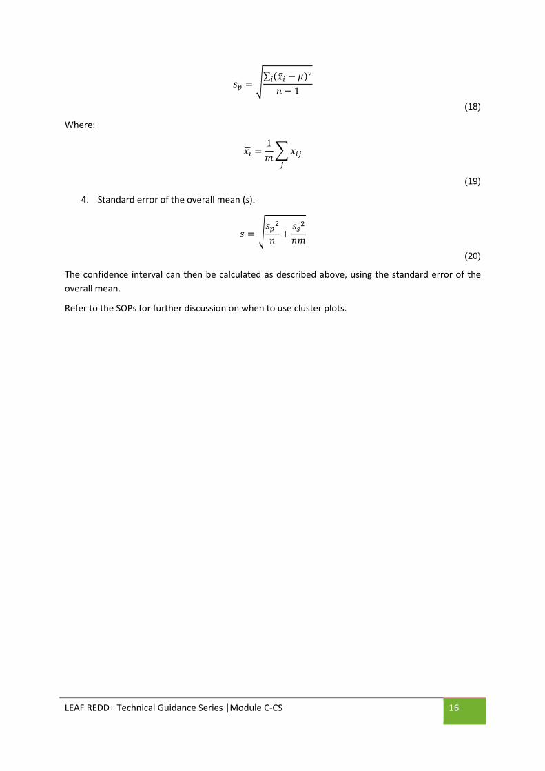
4. Standard error of the overall mean (s).

𝑠 = �𝑠𝑝2

𝑛+𝑠𝑠2

𝑛𝑚

(20)

The confidence interval can then be calculated as described above, using the standard error of the overall mean.

Refer to the SOPs for further discussion on when to use cluster plots.


Calculation of Density from Wood Samples

When calculations require density, and there are no reliable values available from existing literature, it is necessary to calculate density using samples collected in the field. This is usually the case for standing and lying deadwood, and may be the case for biomass calculated from destructive sampling. The SOPs fully describe the collection of samples; this section provides methods to calculate density based on volume and dry weight of samples.


• Dimensions of sample discs: two measurements each of diameter and width.

Equipment required to complete analysis:

• Laboratory scale • Drying oven

Calculation Steps:

1. Calculate the volume of each disc

𝑉𝑜𝑙 = 𝜋 ∗ �𝐷12 + 𝐷2

22

�

2

∗ �𝑇1 + 𝑇2

2�

(21)

Where:

Vol = volume (cm3) D1, D2 = diameter 1 and diameter 1 (cm) T1, T2 = thickness 1 and thickness 2 (cm)

2. In the laboratory, dry discs to a constant weight. Place samples in a proper drying oven at 70°C until sample reaches constant weight over multiple days. Weigh the sample (g) to obtain its dry weight.

3. Calculate density of sample:

𝐷𝑒𝑛𝑠 =𝐷𝑊𝑠𝑎𝑚𝑝𝑙𝑒

𝑉𝑜𝑙

(22)

Where:

Dens = density (g cm-3) DWsample = dry weight (g) Vol = volume (cm3)

4. If multiple samples were taken, repeat steps 1-3 for each sample and average density across all samples.


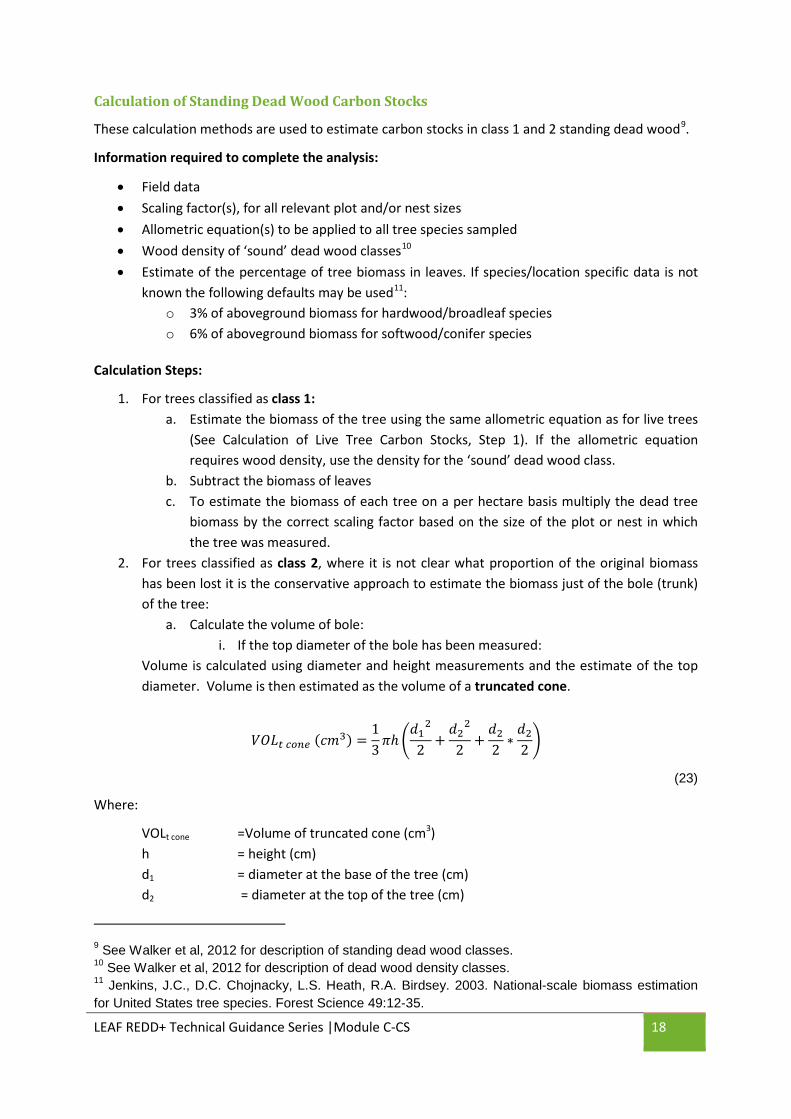
Calculation of Standing Dead Wood Carbon Stocks

These calculation methods are used to estimate carbon stocks in class 1 and 2 standing dead wood9.


• Field data • Scaling factor(s), for all relevant plot and/or nest sizes • Allometric equation(s) to be applied to all tree species sampled • Wood density of ‘sound’ dead wood classes10 • Estimate of the percentage of tree biomass in leaves. If species/location specific data is not

known the following defaults may be used11: o 3% of aboveground biomass for hardwood/broadleaf species o 6% of aboveground biomass for softwood/conifer species

Calculation Steps:

1. For trees classified as class 1: a. Estimate the biomass of the tree using the same allometric equation as for live trees

(See Calculation of Live Tree Carbon Stocks, Step 1). If the allometric equation requires wood density, use the density for the ‘sound’ dead wood class.

b. Subtract the biomass of leaves c. To estimate the biomass of each tree on a per hectare basis multiply the dead tree

biomass by the correct scaling factor based on the size of the plot or nest in which the tree was measured.

2. For trees classified as class 2, where it is not clear what proportion of the original biomass has been lost it is the conservative approach to estimate the biomass just of the bole (trunk) of the tree:

a. Calculate the volume of bole: i. If the top diameter of the bole has been measured:

Volume is calculated using diameter and height measurements and the estimate of the top diameter. Volume is then estimated as the volume of a truncated cone.

𝑉𝑂𝐿𝑡 𝑐𝑜𝑛𝑒 (𝑐𝑚3) =13𝜋ℎ �

𝑑12

2+𝑑2

2

2+𝑑22∗𝑑22 �

(23)

Where:

VOLt cone =Volume of truncated cone (cm3) h = height (cm) d1 = diameter at the base of the tree (cm) d2 = diameter at the top of the tree (cm)

9 See Walker et al, 2012 for description of standing dead wood classes. 10 See Walker et al, 2012 for description of dead wood density classes. 11 Jenkins, J.C., D.C. Chojnacky, L.S. Heath, R.A. Birdsey. 2003. National-scale biomass estimation for United States tree species. Forest Science 49:12-35.


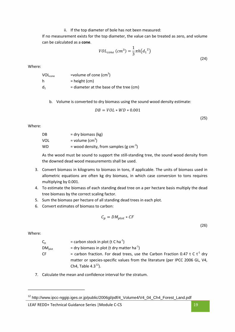
ii. If the top diameter of bole has not been measured: If no measurement exists for the top diameter, the value can be treated as zero, and volume can be calculated as a cone.

𝑉𝑂𝐿𝑐𝑜𝑛𝑒 (𝑐𝑚3) =13𝜋ℎ�𝑑1

2�

(24)

Where:

VOLcone =volume of cone (cm3) h = height (cm) d1 = diameter at the base of the tree (cm)

b. Volume is converted to dry biomass using the sound wood density estimate:

𝐷𝐵 = 𝑉𝑂𝐿 ∗ 𝑊𝐷 ∗ 0.001

(25)

Where:

DB = dry biomass (kg) VOL = volume (cm3) WD = wood density, from samples (g cm-3)

As the wood must be sound to support the still-standing tree, the sound wood density from the downed dead wood measurements shall be used.

3. Convert biomass in kilograms to biomass in tons, if applicable. The units of biomass used in allometric equations are often kg dry biomass, in which case conversion to tons requires multiplying by 0.001.

4. To estimate the biomass of each standing dead tree on a per hectare basis multiply the dead tree biomass by the correct scaling factor.

5. Sum the biomass per hectare of all standing dead trees in each plot. 6. Convert estimates of biomass to carbon:

𝐶𝑝 = 𝐷𝑀𝑝𝑙𝑜𝑡 ∗ 𝐶𝐹

(26)

Where:

Cp = carbon stock in plot (t C ha-1) DMplot = dry biomass in plot (t dry matter ha-1) CF = carbon fraction. For dead trees, use the Carbon Fraction 0.47 t C t-1 dry

matter or species-specific values from the literature (per IPCC 2006 GL, V4, Ch4, Table 4.312).

7. Calculate the mean and confidence interval for the stratum.

12 http://www.ipcc-nggip.iges.or.jp/public/2006gl/pdf/4_Volume4/V4_04_Ch4_Forest_Land.pdf


Standing Deadwood Carbon Stock Example: The table below shows hypothetical data and biomass and carbon calculations for two standing dead trees. For the class 1 tree, biomass is calculated using the Chave equation, as with the live trees. For class 2, biomass is based on the volume calculated for a truncated cone. Density is 0.54.

Class DBH (cm)

Diam at base (cm)

Diam at top (cm)

Height (cm)

Volume (cm3)

Biomass (kg)

Carbon (t)

Scaling factor

Carbon (t/ha)

1 9 N/A N/A N/A N/A 24.92 0.012 198.94 2.33

2 N/A 13.40 1.50 320 16,915 9.13 0.004 198.94 0.85

Total 3.18


Calculation of Lying Dead Wood Carbon Stocks

These calculation methods are used to estimate carbon stocks in lying dead wood for each sampling location measured. These methods assume that the SOP Measurement of Lying Dead Wood and SOP Measurement and Estimation of Dead Wood Density Classes 13 were used to collect field data.


• Field data • Mean wood density of sound, intermediate, and rotten dead wood classes14

Calculation Steps:

1. For each sampling point, the volume of lying dead wood per unit area is estimated using the equation (Warren and Olsen 1964)15 as modified by Van Wagner (1968)16 separately for each density class:

𝑉𝑂𝐿𝐿𝐷𝑊 = 𝜋2 ∗ ��𝑑1

2 + 𝑑22 … 𝑑𝑛

2�8𝐿

�

(27)

Where:

VOLLDW = Volume of lying dead wood per unit area in density class in plot (m3 ha-1) d1…dn = Diameter of piece n of dead wood along the transect in plot (cm) L = Length of the transect in plot (m)

2. Calculate biomass of lying dead wood in each density class and total within each plot:

𝐵𝑀𝐿𝐷𝑊 = � 𝑉𝑜𝑙𝑝𝑙𝑜𝑡,𝑐𝑙𝑎𝑠𝑠

3

𝑑𝑒𝑛𝑠𝑖𝑡𝑦 𝑐𝑙𝑎𝑠𝑠𝑒𝑠∗ 𝐷𝑒𝑛𝑠𝑐𝑙𝑎𝑠𝑠

(28)

Where:

BMLDW = Biomass of lying dead wood per unit area in plot (t dry matter ha-1) Volplot,class = Volume of lying dead wood in density class in plot (m3 ha-1)

Densclass = Mean density of dead wood in the density class (sound, intermediate, and rotten) (t dry matter m-3)

3. Calculate carbon stocks of lying dead wood for each plot by converting from biomass to

carbon:

CSLDW = BMLDW ∗ CFLDW

13 See Walker et al, 2012. 14 See Walker et al, 2012 15 Warren, W.G. and Olsen, P.F. (1964) A line intersect technique for assessing logging waste. Forest Science 10: 267-276. 16 Van Wagner, C.E. (1968). The line intersect method in forest fuel sampling. Forest Science 14: 20-26.


(29)

Where:

CSLDW = Carbon stock of lying deadwood in plot (t C ha-1) BMLDW = Biomass of lying deadwood in plot (t dry matter ha-1) CFLDW = Carbon fraction of dry matter in dead wood (t C t-1 dry matter) (Default

value 0.47 t C t-1 dry matter (per IPCC 2006GL, V4, Ch4, Table 4.317))

Lying Deadwood Carbon Stock Example: The table below shows hypothetical data and biomass and carbon calculations for lying deadwood at one plot, with a transect length of 100 meters.

Decomposition class

Density (g/cm3)

Diameter (cm)

Diameter2

(cm2) Volume (m3/ha)

Biomass (t/ha)

Sound 0.54

16.7 278.89

17.32 9.35

15 225

30 900

Intermediate 0.46 14 196

3.02 1.39 7 49

Rotten 0.21

12 144

81.52 17.12

8 64

80 6400

Sum biomass (t/ha) 27.86

Carbon (t/ha) 13.10

4. Repeat steps for all sampled locations within stratum 5. Calculate the lying dead wood mean and confidence interval for the stratum.



Calculation of Carbon Stocks from Clip Plots

These calculation methods can be used for estimating carbon stocks of all samples collected from a known area such as clip plots. This would include herbaceous vegetation, litter, and non-tree woody vegetation if that vegetation type was sampled in the clip plots.



Calculation Steps:

Using this method, all of the clip plots collected at a sampling location (whether from a single plot of from a cluster of plots) are summed together and treated as one sample.

1. Where the weights recorded in the field include the weight of the bag/sheet and/or subsample bag, calculate the wet weight of the sample and subsample as follows:

𝑊𝑊𝐶𝑃 𝑠𝑎𝑚𝑝𝑙𝑒 = �𝑊𝑏𝑎𝑔𝑡 +𝑚𝑎𝑡𝑒𝑟𝑖𝑎𝑙� − (𝑊𝑏𝑎𝑔)

(30)

𝑊𝑊𝐶𝑃 𝑠𝑢𝑏𝑠𝑎𝑚𝑝𝑙𝑒 = (𝑊𝑠𝑢𝑏𝑠𝑎𝑚𝑝𝑙𝑒 𝑏𝑎𝑔 + 𝑠𝑢𝑏𝑠𝑎𝑚𝑝𝑙𝑒 𝑚𝑎𝑡𝑒𝑟𝑖𝑎𝑙) − (𝑊𝑠𝑢𝑏𝑠𝑎𝑚𝑝𝑙𝑒 𝑏𝑎𝑔)

(31)

Where:

WWCP sample =wet weight of clip plot sample (g) Wbag =weight of bag or sheet (g) WWCP subsample =wet weight of clip plot subsample (g)

Wsubsample bag =weight of subsample bag (g)

2. Create dry-to-wet ratio: a. In the laboratory, dry subsamples to a constant weight. Place samples in a scientific

drying oven at 70oC until sample reaches constant weight over multiple days. b. Weigh the subsample to obtain its dry weight. This dry weight should not include the

weight of the subsample bag. c. Calculate dry-to-wet ratio of subsample:

𝐷𝑊𝑅 =𝐷𝑊𝐶𝑃 𝑠𝑢𝑏𝑠𝑎𝑚𝑝𝑙𝑒

𝑊𝑊𝐶𝑃𝑠𝑢𝑏𝑠𝑎𝑚𝑝𝑙𝑒

(32)

Where:

DWR =Dry-to-wet ratio DWCP subsample =dry weight of clip plot subsample (g)

WWCP subsample =wet weight of clip plot subsample (g)


d. If more than one subsample was taken per sampling location, calculate the mean dry-to-wet ratio for that sampling location

3. Estimate total wet weight of sampled material per sampling location by summing the wet weights of each clip plot sample

4. Using the dry-to-wet ratio, estimate the total dry weight of material for each sampling location:

𝐷𝑊𝐶𝑃 𝑚𝑎𝑡𝑒𝑟𝑖𝑎𝑙 = 𝐷𝑊𝑅 ∗ 𝑊𝑊𝐶𝑃 𝑚𝑎𝑡𝑒𝑟𝑖𝑎𝑙

(33)

Where:

DWCP material =dry weight of clip plot material (g) DWR =Dry-to-wet ratio WWCP material =wet weight of clip plot material (g)

5. Calculate total area sampled within each plot:

TAclip plots = ACP frame ∗ number of CP per sample (34)

Where:

TAclip plots =total area of clip plots (m2) ACP frame =Area of clip plot frame (m2) Number of CP per sample = number of clip plots per sample

6. Calculate scaling factor:

𝑆𝐹 =10,000 𝑚2

𝐶𝑃𝑡𝑜𝑡𝑎𝑙 𝑎𝑟𝑒𝑎 ,𝑝𝑝

(35)

Where:

SF =Scaling factor CPtotal area,pp =Total area of clip plots per plot (m2)

7. Multiply the scaling factor by the total dry mass sampled at one sampling location to obtain dry biomass per hectare.

8. Convert biomass to t C ha-1, using carbon fraction, and 0.001 to convert from kg to tons:

𝐶𝑝 = 𝐷𝑀𝑝 ∗ 𝐶𝐹 ∗ 0.001

(36)

Where:

Cp = carbon stock in plot (t C ha-1) DMp = dry biomass in plot (t dry matter ha-1)


CF = carbon fraction. The IPCC Carbon Fraction default value is 0.47 t C t-1 dry matter (per IPCC 2006GL, V4, Ch4, Table 4.318). Species specific values from the literature may be used if available.

9. Repeat steps for all sampled locations within stratum

10. Calculate mean and uncertainty estimate for all plots for each carbon pool within each stratum.

Clip Plot Carbon Stock Example: The table below shows hypothetical data and calculations for biomass and carbon from clipplots for herbaceous vegetation at one plot. Note that four clip plots were collected and combined.

NB: The calculations are the same for litter plots.

Clip Plot ID

Clip Plot area (m2)

Weight of bag/ plastic sheet (g)

Weight of bag/plastic + vegetation (g)

Wet weight (g)

Weight of bag (g)

Weight of bag + subsample (g)

Wet weight subsample (g)

Dry weight subsample (g)

Dry-wet ratio

Dry weight sample (g)

Scaling factor

AG non-tree biomass (kg/ha)

AG non-tree carbon (tC/ha)

1

1.00

15.00

19.00

4

2

1.00

10.00

140.00

130

3

1.00

15.00

42.00

27

4

1.00

10.00

115.00

105

Total 266

15.00

128.00

113.00 47.1 0.42 110.87 2500

277

0.1386



Calculation of Carbon Stocks from Saplings

Estimating the carbon stocks of saplings requires two sets of measurements: destructively sampling saplings to determine the dry weight of an average sapling and counting saplings within a plot of known area. The average dry weight is used to convert the number of saplings to tons of carbon per hectare. The calculations used are similar to those described for clip plots, with some changes to account for plot measurements entailing the number of saplings rather than the weight.


• Field data of wet weight of saplings from destructive sampling19 • Field data of saplings at field sampling points



Calculation Steps:

A. Calculations to create estimate of ‘average sapling’ weight: These calculations shall be performed on the data collected from destructively sampling saplings.

1. Where the weights of the destructively sampled saplings recorded in the field include the weight of the tarp and/or subsample bag, calculate the wet weight of the sapling and subsample:

𝑊𝑊𝑠𝑎𝑝𝑙𝑖𝑛𝑔 = �𝑊𝑡𝑎𝑟𝑝 + 𝑚𝑎𝑡𝑒𝑟𝑖𝑎𝑙� − (𝑊𝑡𝑎𝑟𝑝)

(37)

Where:

WWsapling =wet weight of sapling (g) Wtarp =tarp weight (g)

𝑊𝑊𝑠𝑢𝑏𝑠𝑎𝑚𝑝𝑙𝑒 = �𝑊𝑠𝑢𝑏𝑠𝑎𝑚𝑝𝑙𝑒 𝑏𝑎𝑔 + 𝑠𝑢𝑏𝑠𝑎𝑚𝑝𝑙𝑒 𝑚𝑎𝑡𝑒𝑟𝑖𝑎𝑙� − (𝑊𝑠𝑢𝑏𝑠𝑎𝑚𝑝𝑙𝑒 𝑏𝑎𝑔)

(38)

Where:

WWsubsample =wet weight of subsample (g) Wsubsample bag =weight of subsample bag (g)

2. Create dry-to-wet ratio: a. In the laboratory, dry subsamples to a constant weight. Place samples in

proper drying oven at 70°C until sample reaches constant weight over multiple days.

19 See SOP Destructive sampling of trees, saplings, palms, and bamboo in Walker et al, 2013


b. Weigh the subsample to obtain its dry weight. This dry weight should not include the weight of the subsample bag.

c. Calculate dry-to-wet ratio of subsample:

𝐷𝑊𝑅 =𝐷𝑊𝑠𝑢𝑏𝑠𝑎𝑚𝑝𝑙𝑒

𝑊𝑊𝑠𝑢𝑏𝑠𝑎𝑚𝑝𝑙𝑒

(39)

Where:

DWR =dry-to-wet ratio DWsubsample =dry weight of subsample (g) WWsubsample =wet weight of subsample (g)

3. Calculate the dry weight of each sapling:

𝐷𝑊𝑠𝑎𝑝𝑙𝑖𝑛𝑔 = 𝐷𝑊𝑅 ∗𝑊𝑊𝑠𝑎𝑝𝑙𝑖𝑛𝑔

(40)

Where:

DWsapling =dry weight of sapling (g) DWR =dry-to-wet ratio

WWsapling =wet weight of sapling (g)

4. Divide by 1,000 to convert to kilograms.

5. Repeat for all saplings destructively sampled

6. Calculate the mean and confidence interval of the ‘average sapling’ for the stratum.

B. Calculations to estimate Carbon stock of Saplings These calculations are to be used to estimate the carbon stock of saplings from field data collected in subplots on the number of saplings per sapling subplot.

1. Multiple the ‘average sapling’ weight by the number of saplings counted in each plot, to obtain kilograms of dry biomass per plot.

2. Calculate scaling factor:

𝑆𝐹 =10,000𝑚2

𝑇𝐴𝑠𝑎𝑝𝑙𝑖𝑛𝑔 𝑝𝑙𝑜𝑡

(41)

Where:

SF =scaling factor TAsapling plot =total area of sampling plot (m2)

3. Multiply the scaling factor by the kilograms of biomass per plot to obtain dry biomass per hectare from each plot.


4. Convert biomass to t C ha-1, using carbon fraction, and 0.001 to convert from kg to tons:

𝐶𝑝 = 𝐷𝑀𝑝 ∗ 𝐶𝐹 ∗ 0.001

(42) Where:

Cp = carbon stock in plot (t C ha-1) DMp = dry biomass in plot (t dry matter ha-1)

CF = carbon fraction. The IPCC Carbon Fraction default value is 0.47 t C t-1 dry matter (per IPCC 2006GL, V4, Ch4, Table 4.320). Species specific values from the literature may be used if available.

5. Repeat steps for all plots within stratum

6. Calculate mean and uncertainty estimate for all plots for each carbon pool within each stratum

Sapling Carbon Stock Example: The table below shows hypothetical data and calculations for saplings from one plot.

Number of saplings

Radius of sampling plot (m)

Sapling plot area (m2)

Scaling factor

Average Dry weight of sapling (kg)

Sapling biomass (kg/ha)

Sapling carbon (t C/ha)

17 2 12.57 795.77 0.33 4464.30 2.10



Calculation of Soil Carbon Stocks

These calculation methods are used to estimate the carbon content in soil in tons per hectare. The SOP “Sampling Soil Carbon” addresses the methods used for soil sampling as well as the laboratory requirements for treating collected samples.


• Field data to estimate soil carbon content • Field data to estimate bulk density • Laboratory analysis of carbon concentration of soil samples

Equipment required to complete the analysis:


Calculation Steps:

1. Calculate the bulk density of the mineral soil core: Dry bulk density soil samples in drying oven at 105° C for a minimum of 48 hours.

𝐵𝐷 = 𝐷𝑀

𝑉𝑂𝐿𝑐𝑜𝑟𝑒 − �𝑀𝑐𝑜𝑎𝑟𝑠𝑒 𝑓𝑟𝑎𝑔𝐷𝑒𝑛𝑠𝑟𝑜𝑐𝑘 𝑓𝑟𝑎𝑔

�

(43)

Where:

BD =bulk density (g/cm3) DM =dry mass (g/cm3) VOLcore =mineral soil core volume (cm3) Mcoarse frag =mass of coarse fragments (g) Densrock frag =density of rock fragments (g/cm3)

Note, bulk density is for the < 2mm fraction, coarse fragments are > 2 mm. The density of rock fragments is often given as 2.65 g/cm3.

2. Using the carbon concentration data obtained from the laboratory, the amount of carbon per unit area is given by:

𝐶 = [(𝐵𝐷𝑠𝑜𝑖𝑙) ∗ 𝐷𝑒𝑝𝑡ℎ𝑠𝑜𝑖𝑙 ∗ 𝐶)] ∗ 100

(44)

Where:

C = carbon (t/ha) BDsoil =soil bulk density (g/cm3) Depthsoil =soil depth

In this equation C must be expressed as a decimal fraction; e.g. 2.2 % carbon is expressed as 0.022 in the equation.


3. Calculate mean soil carbon stock for each plot

4. Repeat steps for all plots within stratum

5. Calculate mean and uncertainty estimate for all plots within carbon pool within each stratum

Soil Carbon Stock Example: The table below shows hypothetical data and calculations for soil samples from one plot.

Bulk density sample ID#

BD sample volume (cm3)

BD sample weight (g)

Bulk density (g/cm3)

Soil C sample ID #

Sample depth (cm)

% Carbon

Carbon (t/ha)

1BD 142.6 250.2 1.75 1SC 30 3.99% 210.02


Wood Products

When trees removed during deforestation result in milled timber or exported logs, the carbon stocks stored in wood products following harvest, Cwp, are based on the efficiency of wood production, or the fraction of biomass effectively emitted to the atmosphere during production. This varies by wood product, location, and mill. It is therefore highly recommended that specific values be obtained for individual countries based on the country’s mill efficiency and the proportion of specific wood products. In the absence of a country-specific value, it is recommended that a literature search be conducted to identify an appropriate figure. Alternately, a common conservative assumption is an overall efficiency of 50%.


• Volume harvested by relevant wood product class • Efficiency factors • Wood density for harvested wood

Calculation Steps:

Multiple the efficiency factors by the volume that goes to each wood product class and the wood density, and sum across classes:

𝐶𝑤𝑝 = �(𝑉𝑜𝑙𝑤𝑝𝑐 ∗ 𝑊𝐷 ∗ 𝐸𝐹𝑤𝑝𝑐) ∗ 0.47

(45)

Where:

Cwp = carbon stock in wood products following deforestation (t C ha−1) Volwpc = volume harvested (m3/ha) by wood product class WD = density of harvested wood (dimensionless) EFwpc = efficiency factor by wood product class (default of 50%, or justified by citation) 0.47 = carbon fraction

The method used here is conservative for wood products from deforestation. A less conservative, but more thorough accounting method would include a decay rate for wood products over time.


Total Biomass Carbon Stocks and Propagation Uncertainty

Calculating Total Carbon Stocks

To estimate the total amount of carbon stocks within a stratum, simply sum the carbon stocks in all measured pools. To convert tons of carbon to tons of carbon dioxide equivalence, simply multiply by the atomic weight difference between C and CO2 (44/12).

If a specific methodology or standard is used, this may delineate how total carbon stocks should be summed. For example, there may be a need to report live aboveground biomass, live belowground biomass, dead biomass, and soil.

𝐶𝑡𝑜𝑡𝑎𝑙 = 𝐶𝐴𝐺−𝑡𝑟𝑒𝑒 + 𝐶𝐵𝐺−𝑡𝑟𝑒𝑒 + 𝐶𝑠𝑎𝑝𝑙𝑖𝑛𝑔 + 𝐶𝑁𝑜𝑛−𝑡𝑟𝑒𝑒𝑊𝑜𝑜𝑑𝑦 + 𝐶𝑁𝑜𝑛−𝑤𝑜𝑜𝑑𝑦𝑉𝑒𝑔 + (𝐶𝑆𝑡𝑎𝑛𝑑𝑖𝑛𝑔𝐷𝑒𝑎𝑑+ 𝐶𝐿𝑦𝑖𝑛𝑔𝐷𝑒𝑎𝑑 + 𝐶𝐿𝑖𝑡𝑡𝑒𝑟)

(46)

𝐶𝑂2𝑒𝑡𝑜𝑡𝑎𝑙 = 𝐶𝑡𝑜𝑡𝑎𝑙 ∗ 4412

(47)

Where:

CO2etotal = Carbon dioxide equivalent within all measured pools (t CO2-e ha-1) Ctotal = Carbon stocks within all measured pools (t C ha-1) CAG-tree = Carbon stocks within aboveground tree pool (t C ha-1) CBG-tree = Carbon stock within belowground tree pool (t C ha-1) Csapling = Carbon stocks within sapling pool (t C ha-1) CNon-treeWoody = Carbon stocks within non-tree woody pool (t C ha-1) Cnon-woodyVeg = Carbon stocks within non-woody vegetation pool (t C ha-1) CStandingDead = Carbon stocks within standing dead tree pool (t C ha-1) CLyinggDead = Carbon stocks within lying dead tree pool (t C ha-1) CLitter = Carbon stocks within litter pool (t C ha-1) 44/12 = Conversion factor to convert Carbon into Carbon Dioxide Considerations for Emission Factor Creation

In instances where total carbon stock data will be used to create emission factors resulting from changing between strata and/or land cover classes, soil carbon should not be included in the sum of carbon stocks. This is because it is often assumed that the changes in soil carbon emissions resulting from deforestation will take place over a 20 year period, based on post-deforestation land use. Therefore, emissions from soil carbon will be accounted for separately.

Again, when total carbon stock data will be used to create emission factors, the wood product pool will be incorporated into the emission factors, with the carbon stored in long-term wood products subtracted from the carbon emissions.


Non-CO2 emissions are also incorporated into the emission factors, by adding these emissions to the emissions from loss of biomass carbon stocks. These calculations are explained in detail in the EF-D module on calculating emission factors for deforestation.21

Uncertainty Propagation

For both total carbon stocks and complete emission factors, it is necessary to propagate the uncertainty estimated for each individual component, and thereby estimate the total uncertainty. This can be done using a Tier 1 method of Simple Propagation of Errors or a Tier 2 method of a Monte Carlo simulation.

Simple Propagation of Errors

Following the methods for simple propagation of errors is appropriate under the following conditions:

• The uncertainties are relatively small, the standard deviation divided by the mean value being less than 0.3;

• The uncertainties have Gaussian (normal) distributions; • The uncertainties have no significant covariance.

When uncertainties are combined by addition or subtraction, such as is the case for summing total carbon stocks, or determining emission factors by subtracting post-deforestation stocks from pre-deforestation stocks including soil carbon emissions and removals in wood products, the following equation is used:

𝑈𝑡𝑜𝑡𝑎𝑙 =�(𝑈1 ∗ 𝑥1)2 + (𝑈2 ∗ 𝑥2)2 + ⋯+ (𝑈𝑛 ∗ 𝑥𝑛)2

|𝑥1 + 𝑥2 + ⋯+ 𝑥𝑛|

(48)

Where:

Utotal = total uncertainty Un = uncertainty associated with each pool, in percent xn = average (mean) of each pool

When uncertainties are combined by multiplication, as when emission factors are multiplied by activity data to estimate total emissions, the following equation is used:

𝑈𝑡𝑜𝑡𝑎𝑙 = �𝑈12 + 𝑈22 + ⋯+ 𝑈𝑛2

(49)

21 Available at: http://leafasia.org/tools/technical-guidance-series-emission-factors-deforestation

http://leafasia.org/tools/technical-guidance-series-emission-factors-deforestation


Total Biomass Carbon Stocks Example: The table below shows hypothetical data and calculations for total biomass across 15 plots. Uncertainty is calculated using simple propagation of errors. (Note that plot 1 shows data from previous examples for each carbon pool.)

Plot

Trees - AGB (tC/ha)

Trees - BGB (tC/ha)

Standing Dead (tC/ha)

Lying Dead (tC/ha)

Clip plot (tC/ha)

Saplings (tC/ha)

All Pools (tC/ha)

1 94.6 22.2 3.2 13.1 0.1 2.1 135.4 2 205.1 48.2 0.7 5.6 0.3 3.2 263.1 3 134.7 31.7 3.2 2.9 0.8 1.3 174.4 4 178.2 41.9 1.3 7.1 0.8 1.7 231.1 5 130.4 30.6 1.7 28.7 0.4 0.3 192.2 6 175.7 41.3 0.3 9.5 0.7 3.2 230.8 7 215.5 50.6 3.2 13.8 0.9 1.5 285.5 8 213.5 50.2 1.5 22.8 0.1 7.0 295.1 9 191.0 44.9 7.0 6.2 0.5 0.5 250.0 10 144.4 33.9 0.5 6.7 0.7 2.1 188.3 11 187.1 44.0 1.3 4.7 0.4 0.1 237.6 12 160.8 37.8 0.1 9.3 0.5 3.2 211.7 13 132.9 31.2 3.0 13.7 1.0 1.5 183.3 14 158.7 37.3 1.5 14.9 0.7 1.7 214.8 15 173.0 40.7 1.7 17.3 0.4 1.3 234.5 Mean 166.4 39.1 2.0 11.8 0.6 2.1 221.9 St Dev 34.4 8.1 1.7 7.1 0.3 1.7 95% CI 19.1 4.5 1.0 4.0 0.1 0.9 CI as % of mean 11.5% 11.5% 47.8% 33.6% 25.3% 45.3% 9.0%

Monte Carlo Analysis

When the conditions listed above are not met, it is necessary to use a numerical statistical technique, such as Monte Carlo analysis to estimate uncertainty. Such a method should be used under the following conditions:

• Uncertainties are large; • Their distribution are non-Gaussian; • The algorithms are complex functions; • Correlations occur between some of the activity data sets, emission factors, or both.

Monte Carlo analysis is method for iteratively evaluating a deterministic model using sets of random numbers as inputs. The analysis uses a computer model to repeatedly perform relevant calculations, numerous times, each time randomly substituting model parameters with a user-defined a range of values for any factor with uncertainty, creating a stochastic model. Because distribution is rarely normal and correlations almost always exist between various measured carbon pools and between estimates at different times it is highly preferable to use this method for propagation of uncertainty, if possible. It generates a total uncertainty distribution consistent with the input uncertainty


distributions of the model parameters, emission factors, and activity data, thereby improving estimates of uncertainty, resulting in a Tier 2 method.

Monte Carlo analysis requires an excel add-in, commercial software, or programming language. Most available products are quite expensive, and all require a learning curve. Listed here are the most common products, along with websites and costs.

• RiskSim, http://www.treeplan.com/, $59 • Oracle Crystal Ball, www.crystalball.com, $995 • @RISK, www.palisade.com, $1,595 • Risk Solver, www.solver.com/risksolver.htm, $3,330

http://www.treeplan.com/

http://www.crystalball.com/

http://www.palisade.com/

http://www.solver.com/risksolver.htm


Other Calculations

Tree Biomass from Destructive Sampling

Destructive sampling of trees may be conducted to validate existing or develop new allometric equations. This section provides the necessary calculations to calculate tree biomass based on data collected during destructive sampling. Consult the SOPs for guidance on how to conduct destructive sampling. The steps required to validate or develop allometric equations are outside the scope of this module.


• Field data of relevant parameters, including tree species and DBH • Field data of volume and/or wet weight for relevant tree components: bole, stump, buttress,

leaves, and branches22. • Wood density for each relevant tree component

Calculation Steps:

1. Calculate the biomass of the bole: A. Calculate the total volume of the bole by summing the volume of all of the sections.

Note that the volume of each section is calculated using the equation for the volume of a frustrum.

𝑉𝑂𝐿 = �13∗ 𝜋 ∗ 𝐿 ∗ ��

𝐷𝑇2�2∗ (𝐷𝑇 ∗ 𝐷𝐵) ∗ �

𝐷𝐵2�2� ∗ 10−6

(50) Where:

VOL = volume (m3) L = length (cm) DT = top diameter of section (cm) DB = bottom diameter of section (cm)

B. Use the density (calculated or found in literature) and the volume to calculate the biomass:

𝐷𝑊𝑏𝑜𝑙𝑒 = 𝐷𝑒𝑛𝑠 ∗ 𝑉𝑜𝑙 ∗ 1000

(51)

Where:

DWbole = biomass of the bole (kg) Dens = bole density (g cm-3) Vol = volume (m3)

2. Calculate the biomass of the stump, based on weight (A), volume (B), or a combination of weight and volume (C).

22 See SOP Destructive sampling of trees, saplings, palms, and bamboo in Walker et al, 2013.


A. To calculate biomass by weight multiply total wet weight by the dry-to-wet ratio obtained by drying samples.

𝐷𝑊𝑠𝑡𝑢𝑚𝑝,𝑤 = �𝐹𝑊𝑖 ∗ 𝐷𝐹𝑅

(52)

Where:

DWstump,w = biomass of the stump (kg), calculated by weight

WWi = wet weight (kg) of pieces of the stump, as scale allows

DWR = dry-to-wet ratio, determined by taking the fresh and oven-dried weight of at least three subsamples, finding the ratio, and averaging across all samples

B. To calculate biomass by volume, identify the shape the stump most closely resembles, frustrum, cube, or cylinder, use the appropriate volume equation, and multiply the volume by wood density.

𝐷𝑊𝑠𝑡𝑢𝑚𝑝,𝑣 = 𝑉𝑂𝐿 ∗ 𝑊𝐷 ∗ 1000 (53)

Where:

DWstump,v = biomass of the stump (kg), calculated by volume

VOL = volume (m3)

WD = wood density (g cm-3)

Where volume is calculated based on shape:

For Cube: 𝑉𝑐𝑢𝑏𝑒 (𝑚3) = 𝐿𝑒𝑛𝑔𝑡ℎ (𝑚) ∗𝑊𝑖𝑑𝑡ℎ (𝑚) ∗ 𝐻𝑒𝑖𝑔ℎ𝑡 (𝑚) (54)

For Cube: 𝑉𝑐𝑦𝑙𝑖𝑛𝑑𝑒𝑟 (𝑚3) = 𝜋 ∗ 𝑟𝑎𝑑𝑖𝑢𝑠2 (𝑚) ∗ 𝐻𝑒𝑖𝑔ℎ𝑡 (𝑚) (55)

For Frustrum: 𝑉𝑓𝑟𝑢𝑠𝑡𝑟𝑢𝑚 (𝑚3) = 13∗ 𝜋 ∗ 𝐻𝑒𝑖𝑔ℎ𝑡 (𝑚) ∗ 𝐿𝑎𝑟𝑔𝑒𝑅𝑎𝑑𝑖𝑢𝑠 (𝑚) ∗ 𝑆𝑚𝑎𝑙𝑙𝑠𝑅𝑎𝑑𝑖𝑢𝑠 (𝑚)

(56)

C. To calculate biomass by both weight and volume, simply calculate DWstump,w and

DWstump,v and sum them. This is useful when it is easier to take volume measurements for some of the stump and weight measurements for the rest.

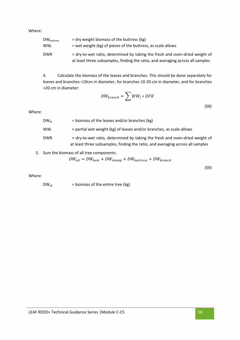
3. Calculate the biomass of the buttress:

𝐷𝑊𝑏𝑢𝑡𝑡𝑟𝑒𝑠𝑠 = �𝑊𝑊𝑖 ∗ 𝐷𝐹𝑅

(57)


Where:

DWbuttress = dry weight biomass of the buttress (kg) WWi = wet weight (kg) of pieces of the buttress, as scale allows


4. Calculate the biomass of the leaves and branches. This should be done separately for leaves and branches <10cm in diameter, for branches 10-20 cm in diameter, and for branches >20 cm in diameter:

𝐷𝑊𝑏𝑟𝑎𝑛𝑐ℎ = �𝑊𝑊𝑖 ∗ 𝐷𝐹𝑅

(58) Where:

DWlb = biomass of the leaves and/or branches (kg)

WWi = partial wet weight (kg) of leaves and/or branches, as scale allows


5. Sum the biomass of all tree components. 𝐷𝑊𝑎𝑙𝑙 = 𝐷𝑊𝑏𝑜𝑙𝑒 + 𝐷𝑊𝑠𝑡𝑢𝑚𝑝 + 𝐷𝑊𝑏𝑢𝑡𝑡𝑟𝑒𝑠𝑠 + 𝐷𝑊𝑏𝑟𝑎𝑛𝑐ℎ

(59)

Where:

DWall = biomass of the entire tree (kg)


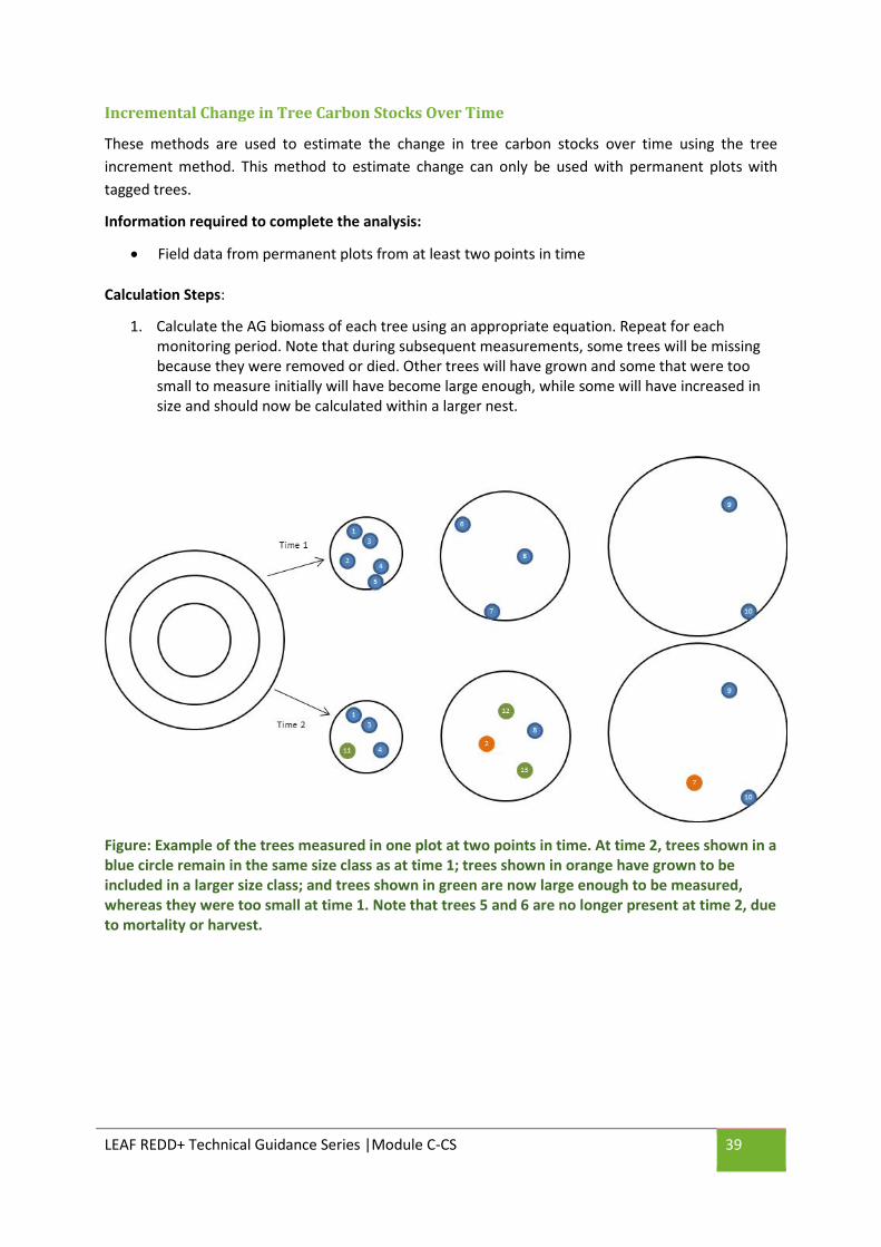
Incremental Change in Tree Carbon Stocks Over Time

These methods are used to estimate the change in tree carbon stocks over time using the tree increment method. This method to estimate change can only be used with permanent plots with tagged trees.


• Field data from permanent plots from at least two points in time

Calculation Steps:

1. Calculate the AG biomass of each tree using an appropriate equation. Repeat for each monitoring period. Note that during subsequent measurements, some trees will be missing because they were removed or died. Other trees will have grown and some that were too small to measure initially will have become large enough, while some will have increased in size and should now be calculated within a larger nest.

Figure: Example of the trees measured in one plot at two points in time. At time 2, trees shown in a blue circle remain in the same size class as at time 1; trees shown in orange have grown to be included in a larger size class; and trees shown in green are now large enough to be measured, whereas they were too small at time 1. Note that trees 5 and 6 are no longer present at time 2, due to mortality or harvest.


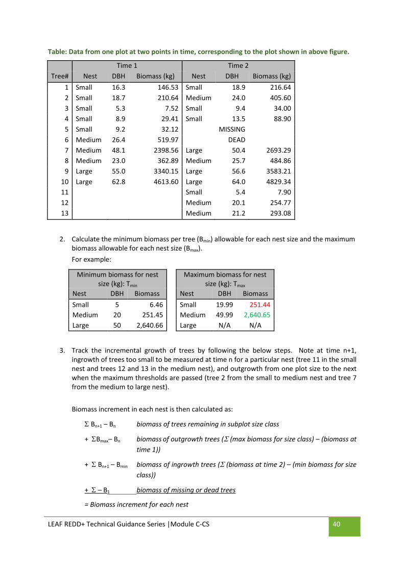
Table: Data from one plot at two points in time, corresponding to the plot shown in above figure.

Time 1 Time 2 Tree# Nest DBH Biomass (kg) Nest DBH Biomass (kg)

1 Small 16.3 146.53 Small 18.9 216.64 2 Small 18.7 210.64 Medium 24.0 405.60 3 Small 5.3 7.52 Small 9.4 34.00 4 Small 8.9 29.41 Small 13.5 88.90 5 Small 9.2 32.12 MISSING 6 Medium 26.4 519.97 DEAD 7 Medium 48.1 2398.56 Large 50.4 2693.29 8 Medium 23.0 362.89 Medium 25.7 484.86 9 Large 55.0 3340.15 Large 56.6 3583.21

10 Large 62.8 4613.60 Large 64.0 4829.34 11

Small 5.4 7.90

12

Medium 20.1 254.77 13 Medium 21.2 293.08

2. Calculate the minimum biomass per tree (Bmin) allowable for each nest size and the maximum biomass allowable for each nest size (Bmax). For example:

Minimum biomass for nest size (kg): Tmin

Maximum biomass for nest size (kg): Tmax

Nest DBH Biomass

Nest DBH Biomass Small 5 6.46

Small 19.99 251.44

Medium 20 251.45

Medium 49.99 2,640.65 Large 50 2,640.66

Large N/A N/A

3. Track the incremental growth of trees by following the below steps. Note at time n+1, ingrowth of trees too small to be measured at time n for a particular nest (tree 11 in the small nest and trees 12 and 13 in the medium nest), and outgrowth from one plot size to the next when the maximum thresholds are passed (tree 2 from the small to medium nest and tree 7 from the medium to large nest). Biomass increment in each nest is then calculated as:

Σ Bn+1 – Bn biomass of trees remaining in subplot size class

+ ΣBmax– Bn biomass of outgrowth trees (Σ (max biomass for size class) – (biomass at time 1))

+ Σ Bn+1 – Bmin biomass of ingrowth trees (Σ (biomass at time 2) – (min biomass for size class))

+ Σ – B1 biomass of missing or dead trees

= Biomass increment for each nest


(60)

Where:

Bn = biomass of tree at time n

Bn+1 = biomass of tree at time n+1

Bmax = maximum biomass allowable in nest size

Bmin = minimum biomass allowable in nest size

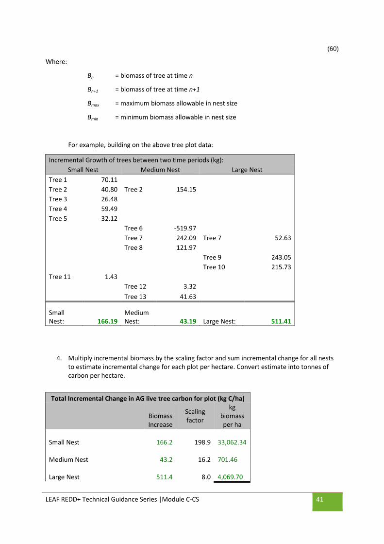
For example, building on the above tree plot data:

Incremental Growth of trees between two time periods (kg): Small Nest Medium Nest Large Nest

Tree 1 70.11 Tree 2 40.80 Tree 2 154.15

Tree 3 26.48

Tree 4 59.49

Tree 5 -32.12

Tree 6 -519.97

Tree 7 242.09 Tree 7 52.63

Tree 8 121.97

Tree 9 243.05

Tree 10 215.73

Tree 11 1.43

Tree 12 3.32

Tree 13 41.63

Small Nest: 166.19

Medium Nest: 43.19 Large Nest: 511.41

4. Multiply incremental biomass by the scaling factor and sum incremental change for all nests to estimate incremental change for each plot per hectare. Convert estimate into tonnes of carbon per hectare.

Total Incremental Change in AG live tree carbon for plot (kg C/ha)

Biomass Increase

Scaling factor

kg biomass per ha

Small Nest 166.2 198.9 33,062.34

Medium Nest 43.2 16.2 701.46

Large Nest 511.4 8.0 4,069.70


Total Increase in AG Biomass for plot (kg/ha): 37,833.50

Total Increase in AG tree Carbon for plot (tC/ha): 17.78

5. Calculate the incremental change in belowground carbon. a. Calculate AG Biomass of plot using allometric equation and expansion factors for time n b. Calculate incremental increase in AG biomass as explained above c. Add incremental increase in AG biomass to biomass at time n d. Apply root biomass equation to this biomass to estimate BG Biomass at time n+1 e. BG Carbon at time n+1 - BG Carbon at time n = incremental change in BG Carbon.

Carbon (t C/ha)

Above ground Below ground

Time 2 94.7 + 17.8 = 112.4 26.4

Time 1 94.7 22.2

Incremental Change in BG tree C for plot (t C/ha): 4.2

6. Repeat for each plot and then calculate the mean incremental change and 95% CI for each stratum. Multiply by area of stratum, and sum total change in C for all stratum.

Ecosystem Services Winrock International

[email protected]

+1.703.302.6500

2121 Crystal Drive, Suite 500

Arlington, VA 22202, USA

www.winrock.org

module c-cs: calculations for estimating carbon stocks · leaf technical guidance series for the...

Documents