module 8 use of double geography datasets within saspac

Module 8

Use of Double Geography

datasets within SASPAC

SASPAC Training Double Geography datasets

Module 8 Page 119

Introduction The ‘standard’ datasets supplied by the Census Offices are one-dimensional in a geographic sense in that each item of information is related to a single area. That is why they are occasionally referred to as single geography datasets. The CSV file as supplied consists of a series of records (or lines), each of which is a series of numbers associated with a single area code and (possibly) one area name. A part of the CSV file for table UV002 is shown here: "00GANY0001",238,3,70.00

"00GANY0002",294,5,65.33

"00GANY0003",280,11,25.66

"00GANY0004",300,12,24.61

"00GANY0005",271,6,45.09

On the other hand, the ‘special’ datasets supplied by the ONS are geographically two-dimensional as each item of data is linked to two areas. In the migration datasets, the two areas are the area of residence one year prior to the census, and the area of residence at census day, while in the workplace (or in Scotland, travel) datasets, the areas are area of residence, and area of workplace (both at census day). These datasets are referred to as double geography datasets. As with the single geography datasets, the CSV file supplied consists of a series of records each of which is a series of numbers associated with two area codes and (possibly) two area names. A part of the CSV file for table SMS301 is shown here: “20UEGL0006”,”20UEGF0017”,3,3,0,0,0,0,3,3,0,0,0,0

“20UEGL0006”,”20UEGF0019”,3,3,0,0,0,0,3,3,0,0,0,0

“20UEGL0006”,”20UEGG0006”,3,3,0,0,0,0,3,3,0,0,0,0

“20UEGL0006”,”20UEGG0008”,3,3,0,0,0,0,3,3,0,0,0,0

“20UEGL0006”,”20UEGJ0002”,7,4,3,0,0,0,7,4,3,0,0,0

“20UEGL0006”,”20UEGJ0003”,33,14,19,0,0,0,33,14,19,0,0,0

Apart from the fact that the double geography datasets have two geographic references per area, their record structure is similar to that of the single geography datasets, and SASPAC may be used to access them with a few minor modifications in the appearance of the windows and choices that are offered to the user. For any single variable the dataset may be represented as a two-dimensional matrix – hence the alternative name matrix datasets – with the third dimension then being represented by the other variables. The migration data is available as a United Kingdom dataset, but there are two datasets for workplace related movements. This is because in Scotland the question relating to place of work was extended to cover place of study as well. The two relevant questions in each of the areas was as follows: England, Wales, and Northern Ireland:

Question 33. What is the address of the place where you work in your main job? Question 34. How do you usually travel to work?

Double Geography datasets SASPAC Trainings

Page 120 Module 8

Scotland:

Question 10. What address do you travel to for your main job or course of study (including school)?

Question 11. How do you usually travel to your main place of work or study (including school)?

The ONS released a series of tables under three generic titles: Matrices of journeys to work (Areas of residence in England, Wales, and NI)

Within SASPAC these tables are given the table identifier code SWS. There are 14 tables (plus one Northern Ireland variation). Seven of these – numbered SWS101 to SWS107 – are available at local authority district level; six – numbered SWS201 to SWS206 – are available at ward level; and one – numbered SWS301 – is available at Output Area level.

Matrices of journeys to place of work or place of study (Areas of residence in Scotland)

Within SASPAC these tables are given the table identifier code TVS. There are 14 tables. Seven of these – numbered TVS101 to TVS107 – are available at local authority district level; six – numbered TVS201 to TVS206 – are available at ward and postcode sector level; and one – numbered TVS301 – is available at Output Area level.

Matrices of migration moves

Within SASPAC these tables are given the table identifier code SMS. There are 16 tables (plus one Northern Ireland variation). Ten of these – numbered SMS101 to SMS110 – are available at local authority district level; five – numbered SMS201 to SMS205 – are available at ward level (and postcode sector level in Scotland); and one – numbered SMS301 – is available at Output Area level.

Within the United Kingdom there are some 220,000 Output Areas, and about 10,500 wards. The resulting matrices of area to area moves for each of these levels have the potential to be very large even though not all the combinations of origin zone and destination zone will actually produce a flow. The following table shows the number of origin zones, the number of destination zones, and the actual number of flows for a few of the datasets currently available.

Table Number of origin zones

Number of destination zones

Number of flows

SWS201 9,432 10,223 1,367,170

SMS201 10,610 10,608 851,317

SWS301 175,428 177,404 5,951,376

SMS301 221,468 221,817 1,971,282

As table SWS301 for a single pair of origins/destinations contains 36 cells, the full dataset for this table contains over 200 million cells. A consequence of this is that the data is extremely sparse with most of the cells having a value of zero and many others having very low values. The Small Cell Adjustment Methods (SCAM) applied by ONS and NISRA Census Offices to this data mean that a small count appearing in a table cell is adjusted - information on what constitutes a small cell count cannot be provided as this may compromise confidentiality protection – but


Module 8 Page 121

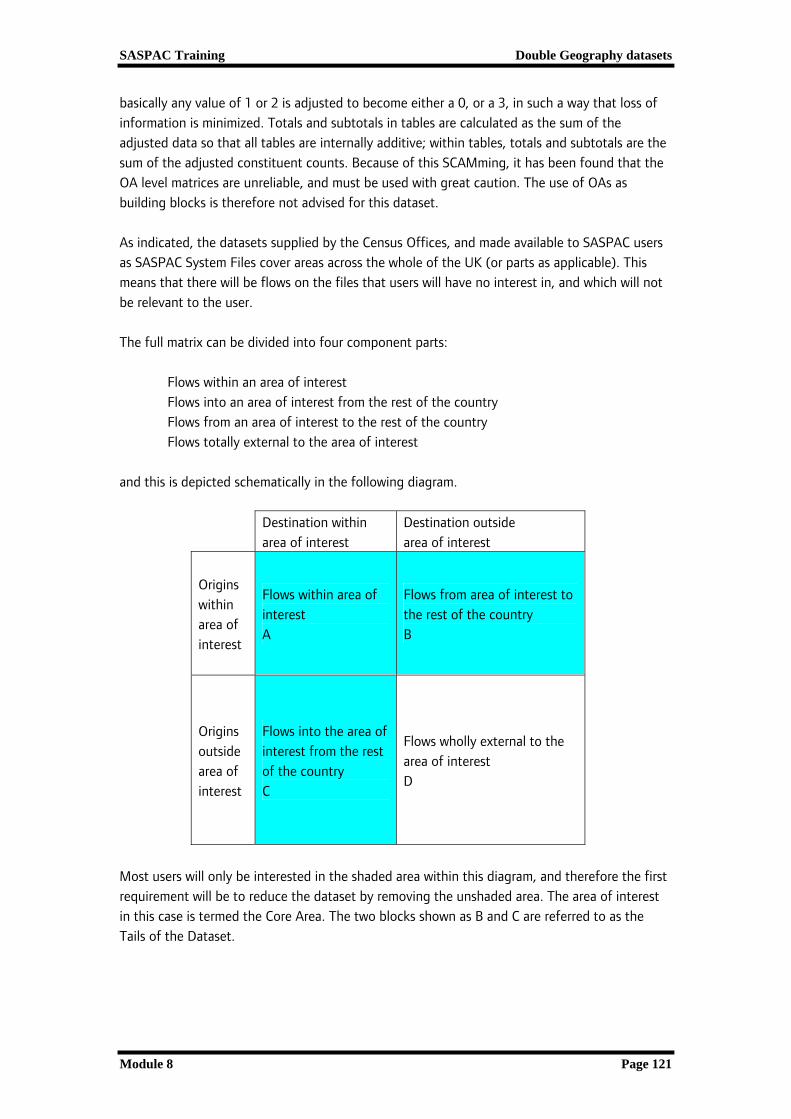
basically any value of 1 or 2 is adjusted to become either a 0, or a 3, in such a way that loss of information is minimized. Totals and subtotals in tables are calculated as the sum of the adjusted data so that all tables are internally additive; within tables, totals and subtotals are the sum of the adjusted constituent counts. Because of this SCAMming, it has been found that the OA level matrices are unreliable, and must be used with great caution. The use of OAs as building blocks is therefore not advised for this dataset. As indicated, the datasets supplied by the Census Offices, and made available to SASPAC users as SASPAC System Files cover areas across the whole of the UK (or parts as applicable). This means that there will be flows on the files that users will have no interest in, and which will not be relevant to the user. The full matrix can be divided into four component parts: Flows within an area of interest Flows into an area of interest from the rest of the country Flows from an area of interest to the rest of the country Flows totally external to the area of interest and this is depicted schematically in the following diagram.

Destination within area of interest

Destination outside area of interest

Origins within area of interest

Flows within area of interest A

Flows from area of interest to the rest of the country B

Origins outside area of interest

Flows into the area of interest from the rest of the country C

Flows wholly external to the area of interest D

Most users will only be interested in the shaded area within this diagram, and therefore the first requirement will be to reduce the dataset by removing the unshaded area. The area of interest in this case is termed the Core Area. The two blocks shown as B and C are referred to as the Tails of the Dataset.


Page 122 Module 8

Creating a sub-set of the origin/destination datasets for zones within an area of interest (or Core Area). For this exercise we shall take the Core Area as being the London Borough of Enfield, and we shall create the data for all Special Workplace Statistics Tables at ward level (2001 SWS2 WARDS TO WARDS.SYS). The requirement is to create a new System File containing only data related to a core area, and so the New System File task window is accessed through use of the File/New Task/Create New System File option, at which point the appropriate national dataset is selected.

Once an origin/destination dataset is selected, the task window changes slightly in that there is an additional tick-box now available as shown in this image. This allows the user to restrict the core area data to only flows within the core area, and all flows with an external component will be excluded.

In terms of the previous diagram, this would mean that only the moves in block A would be included. Above this tick-box under the ‘Variables’ header it is possible to input selected variables to be saved, leaving this blank will automatically save all variables in the original system file.

The selection of the core area zones may now be initiated in the usual way through use of the 'Select Areas' command button on the ‘Create New System File’ main task window. As a double geography file has been selected, the window that is now presented to the user reflects this in that the property sheet has tabs titled 'Origins' and ‘Destinations'.

To view the zones that are on the input file, the 'View Data' command button is clicked, and a full list of the zones found on the input file will be shown. Note that all the area symbols will have a superimposed red 'C'. This indicates that the zone is part of the core area for this file. As it is a national data file all zones are within the core area and will therefore be indicated as such by the red 'C'


Module 8 Page 123

If the core area is to be symmetrical, that is the areas of origin within it are identical to the areas of destination, then the process of area selection may be simplified by clicking the 'Apply to both axes' tick-box. This ensures that the process of zone selection need only be done once. The first zone in the core area is selected by scrolling down the list and clicking on it followed by clicking on 'Include'. The list is then scrolled to the last zone in the area of interest, and by shift-clicking on this zone, the full range may be selected. Note however, that this may take some time, depending on the power of your PC and the number of zones to be included, and it may be faster to simply click on this last zone for inclusion and to edit the command file created as indicated below. [Note: An alternative to scrolling is to use the ‘Find’ button to access a search window into which the user enters a part of the code or name of the area that is to be used. In this case, as the code for Enfield is 00AK, we enter this in the text box, after which use of the ‘Find next’ button will move the selection to the first ward in Enfield – 00AKGL Bowes] Once the zones within the core area (or the start and end zones of the range) have been identified, then the 'Make Command' command button is clicked to generate the appropriate

command(s). The final stage is to allocate an appropriate name and label in the required locations in the task window which appear when the 'Close' command button is clicked. Once this is done, the 'Close' command button on the task window is used to enter the task submission window, at which point the user can allocate an

appropriate command file name. Also, if only the end zones of the range were selected, rather than the range itself, then the 'Save only' radio button on this window must be checked to allow the created command file to be edited as follows: Change the lines which are of the form:

include <startzone_code>

include <endzone_code>

to include <startzone_code> to <endzone_code>

This command file can then be saved and run to produce a system file containing only the flows relevant to the core area. If the Tools/System File Details menu item is now used on this new file, the user will see that only the wards in their area of interest are shown as being part of the Core Area. Other areas will appear as origins and/or destinations, but without the core area indicator, they are automatically parts of the tails of the dataset.


Page 124 Module 8

The System File Details display also shows that there are now 20,194 flows within the dataset arising from 2,581 origins and 1,665 destinations. The file is therefore much more manageable as is also shown by the fact that the original file of 611Mb has been reduced to less than 5.9Mb. Re-zoning areas outside the core area The file that has just been created will contain ward-to-ward flows related to the Enfield core area. As such it will contain, for example, flows with origins in Scottish wards and destinations in Enfield wards. It is however highly probable that the user will not be interested in origins or destinations at such a fine level of detail where the distance involved is very large. In this case, the user will want to create new zones for areas outside the core area The easiest form of external rezoning would see all the external wards aggregated to the local authority district level, although it would be possible to aggregate the more local wards to local authority level, those a little further away to county level, and those further still to region level. To undertake a rezoning of all external wards to local authority districts, we shall use the gazetteer file ‘Ward_to_District.gaz’. This file allocates wards to local authority districts and also provides labels for these districts. It has the existing zone (wards) in columns 1 to 6, and the new zone (districts) in columns 15 to 18, with no scaling factor. To adapt this for use in Enfield, we need to remove all wards in Enfield from the assignment (or second) part of the gazetteer file, and also the Enfield line from the labelling (or first) element of the file. Once this is done we will save the gazetteer file as ‘Ward_to_District_Enfield.gaz’. The first stages of the process are the same as for single geography rezoning, and the “File/New Task/Create New Zones..” route is followed, at which stage the system file created in the previous exercise is selected. The resultant window now differs from the window seen in

Module 7 in that this is double geography specific. There is a block under ‘Method’ which specifies what is to be done with areas on the input system file that are not used in the new zone creation commands – either through Using Areas or Gazetteer Files. As we are

not considering the Enfield wards in the gazetteer file and we want those to appear as they are in the new system file, the ‘Include unused origins and destinations’ button is left checked. As we are going to use a gazetteer file, the ‘Gazetteer Files’ button is used to take us to the next window, which is again different from that seen in Module 7, as it again caters for double geography. The main difference is that this window has two tabs which allow for gazetteer files to be chosen either to apply to both axes together or individually. This is shown in the next


Module 8 Page 125

image. A minor difference is that as hierarchies are not allowed in double geographies, the ‘Zones Hierarchic On’ checkbox has disappeared.

The appropriate input gazetteer file is selected in the usual manner by use of the ‘Input from…’ button. As noted earlier, the existing zone (wards) code is in columns 1 to 6, and the new zone (districts) code is in columns 15 to 18, with no scaling factor. These values are entered into the appropriate boxes. In

addition, the gazetteer file has a label element, and so the ‘With Labels’ box must be checked. For the sake of obtaining a full check on the allocation of zones (wards) in the new zone creation, the ‘Zone Echo On’ box is also checked. The final stage is to allocate a label and name to the output system file and then to run the rezoning task. However, there is currently an issue that must be addressed before this is done and so the file must be saved and closed using the ‘Save Only’ option. As the gazetteer file has been generated from a listing of all ward files, and not all of these wards will appear as origins or destinations on the input system files. By definition, areas that appear on a gazetteer file are expected to appear on the input system file, and their absence will cause an error. This is overcome by use of a command that is used for testing the software, but in this case prevents the absence of the area from creating an error. This command is ‘Test 71’, and this is placed as the first command line in the command file. A check on the System File details reveals that we now have a file in which there are 4,991 flows with 366 origin zones and 310 destination zones, and the file size has been further reduced from 5.9Mb to 1.6Mb.


Page 126 Module 8

Using the origin/destination datasets Once the national dataset has been tailored to the user’s needs as detailed in the previous exercises, it may be used in virtually the same way as any other SASPAC System File. The main difference that the user will notice is that, once a double geography system file has been selected, some windows have a slightly different appearance, as has already been noted. Example For areas of origin and destination in London Borough of Enfield, extract the total numbers of persons, and males and females moving to work wholly within Enfield, and map the total persons within SASPAC. This is a standard mapping task within SASPAC, with the difference that the dataset to be accessed is an origin/destination one. As there is a need to produce a CSV file for the mapping, the start of the task follows the usual File/New Task/Export data/CSV file route. This produces the standard main task window where the user must select the required input file first. Note that whereas with single geography analyses, the input system file may be selected at any time, with double geography, the input system file must be selected at the outset. This is because the functionality available changes slightly when double geography is used. When the double geography file is selected, the amended window shown here will appear. Note that as soon as a double geography System File is selected, the ‘Input System Files’ buttons are greyed out. This is because only one input file is allowed with double geography analyses. Also note the addition of a check box that allows restriction of the analysis to flows wholly within the areas of interest. Checking this box leads to the insertion of the command ‘SET IN&OUT OFF’ in the Command File.

As with single geography, the ‘Select Areas’ command button may be used to select the required areas. However, as the input system file is double geography, radial searching is not an option, and in place of the ‘Explore Zones’ tab, there is a tab each for origin and destination. Additionally, instead of the check boxes for the various


Module 8 Page 127

exclusions associated with single geography, there is now a single check box labelled ‘Apply to both axes’. If this box is checked, selections made in the usual way through either the ‘View Data’ or ‘Use Mapshore’ options will apply to both origin and destination. Otherwise, selections will have to be made twice - once for each of the origin and destination tabs.

With the ‘Apply to both axes’ check-box checked, the areas within the core area may now be selected in the usual manner (remembering to use the ‘Make Command’ button). It is worth remembering that although the use of ‘Shift/click’ for selecting ranges works, sometimes in practice, depending on the size of the file, it can be a

very slow procedure, and the most efficient way is to select the first area in the range, and then select the last area in the range. The commands created by this option may then be edited once the complete command file has been created, through use of the ‘Save only’ radio button in the final Task window. The searching facilities for the double geography datasets can be used to search and select the required variables (NB. Remember to use the ward level SWS dataset to select these). Both the origin (‘ORIGID’) and destination‘(DESTID’) header variable codes will also need to be included at this point although, SASPAC will prompt the user to save these before running the task. Having done this, the output CSV file may be named and the task is run.

Using the ‘Go Mapping’ button in SASPAC will open Mapshore, and we then first open the appropriate boundary file – in this case Enfield wards – followed by the CSV file just created. As the CSV file is a double geography related file, the route to this is through the Data/Desire Line Double Geography option, as shown.

Use of this option will open the usual Windows dialog box where the user navigates to the appropriate drive/directory to find the required file. As there are multiple data items on this file that was created, the system asks which data item is to be mapped. If the variable representing


8 Module 8

the total (SWS2010001) is selected, the map is populated with a large number of arrows which effectively obliterate the whole map. Use of Zoom/Layering Allows the user to control the presentation of the map. This is done by highlighting the Double

Geography file, and then using the ‘Properties’ command button. This brings up the window shown here, in which the user can set arrow widths, arrow colours, and range values. Setting an arrow width to zero will prevent that range from displaying on a map.

Using the settings as shown in the adjacent window, produces a map as shown below. This map

can then be zoomed to examine flow patterns in particular areas. Note that because boundaries are not available for areas outside Enfield, cross boundary flows would not be mapped even if they were present in the CSV file. The mapping depends on the availability of boundary files at the appropriate level.

As with any mapping within Mapshore, this can be annotated with text, and all the other mapping functionality is also available as discussed in Module 5.


Module 8 Page 129

Additional output facilities available only with Double Geography datasets In addition to the usual Print Tables and Print Variables options, there are three other Print options that are only available when a double geography dataset has been input. These are: Print Summary Print Netflow Print Matrix Additionally, it should be noted that Print Profile and Print VarTables are not available with double geography datasets. Each of the three additional options is initiated in exactly the same way as the other Print commands. Print Summary A Print Summary task will print the following for each of the variables selected for output: Row Total The total number for the area as an area of origin, i.e. it is the sum of flows

from that area of origin to all destinations. Column Total The total number for the area as an area of destination, i.e. it is the sum of

flows to that area of destination from all origins Intra The total number of flows within the area, i.e. the area is the area of origin and

destination Row Max The value of the largest flow from the area as an area of origin Row Count The total number of destinations with an origin in the area, and the number of

these with a non-zero value for the selected variable Column Max The value of the largest flow to the area as an area of destination Column Count The total number of origins with a destination in the area, and the number of

these with a non-zero value for the selected variable Sample output from a Print Summary task is shown below.


Page 130 Module 8

Print Netflow A Print Netflow task will print the following for each of the variables selected: Out flow The value for the selected variable of the flow from the first area to the second

area i.e. it is the value when the first area listed is considered as the origin, and the second area is considered as the destination

In flow The value for the selected variable of the flow to the first area from the second

area i.e. it is the value when the first area listed is considered as the destination, and the second area is considered as the origin

Ratio The ratio of the Inflow to the Outflow Net flow The difference between the Inflow and the Outflow Sample output from a Print Netflow task is shown below:

Print Matrix A Print Matrix task will print the matrix of moves between selected zones for the selected variables, with the areas of origin being the rows, and the areas of destination the columns. Sample output from a Print Matrix task is shown below:

Note that the largest values are usually along the diagonal, as they represent the ‘within zone’ flows. Summary of task sequence


Module 8 Page 131

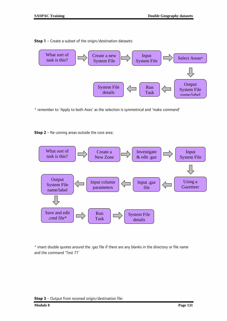
Step 1 – Create a subset of the origin/destination datasets:

* remember to ‘Apply to both Axes’ as the selection is symmetrical and ‘make command’ Step 2 – Re-zoning areas outside the core area:

* insert double quotes around the .gaz file if there are any blanks in the directory or file name and the command ‘Test 71’ Step 3 – Output from rezoned origin/destination file:

Create a new System File

What sort of task is this?

Input System File Select Areas*

Output System File name/label

System File details

Run Task

Create a New Zone


Investigate & edit .gaz

Input System File

Using a Gazetteer

Input column parameters

Input .gaz file

Output System File name/label

Run Task

System File details

Save and edit .cmd file*


Page 132 Module 8

* remember to check the ‘Apply to both axes’ tick box to save making origin/destination selections separately

Output CSV file


Input System File

Select Areas* Output file name

‘Go Mapping’ Run Task

Retrieve boundary file

Search & select

variables

Retrieve Desireline Area file

module 8 use of double geography datasets within saspac

Documents