module 5: visualization - ubc department of statisticswill/cx/private/mod5... · 2014-09-30 ·...
TRANSCRIPT

2 2PIMS
..........
.....
.....................................................................
.....
......
.....
.....
.
Module 5: Visualization
Jerome Sacks and William J. Welch
National Institute of Statistical Sciences and University of British Columbia
Adapted from materials prepared by Jerry Sacks and Will Welch forvarious short courses
Acadia/SFU/UBC Course on Dynamic Computer ExperimentsSeptember–December 2014
J. Sacks and W.J. Welch (NISS & UBC) Module 5: Visualization Computer Experiments 2014 1 / 51

2 2PIMS
..........
.....
.....................................................................
.....
......
.....
.....
.
Outline
Outline of Topics
You have fitted a Gaussian process (GP) model and have y(x) (i.e., m(x)from Module 3). What’s next?Use y(x) instead of y(x) to answer scientific and engineering questions.
..1 Science and Engineering Objectives
..2 Functional Decomposition
..3 Sensitivity Analysis / Screening
..4 Visualization
..5 Case Study: Arctic Sea-Ice Computer Model
..6 Summary
..7 Case Study: Wonderland Computer Model
J. Sacks and W.J. Welch (NISS & UBC) Module 5: Visualization Computer Experiments 2014 2 / 51

2 2PIMS
..........
.....
.....................................................................
.....
......
.....
.....
.
Science and Engineering Objectives
Some Science and Engineering Questions
• Visualization: What do the y(x) input-output relationships look like?
• Sensitivity analysis / screening: What are the important variables?
• Optimization: What values of x maximize/minimize y? (Could havemultiple output variables to optimize simultaneously.)
• Propagation of variation: If x has a known distribution, what is thedistribution of y(x)?
• . . . other questions about y(x)
We are assuming y(x) is too expensive to compute many times to answersuch questions, so . . .
• Replace y(x) with y(x).
J. Sacks and W.J. Welch (NISS & UBC) Module 5: Visualization Computer Experiments 2014 3 / 51

2 2PIMS
..........
.....
.....................................................................
.....
......
.....
.....
.
Functional Decomposition
Visualization and Sensitivity Analysis / Screening
The Visualization and Sensitivity analysis / screening questions can beanswered by decomposing the function into low-dimensional components(one or two input variables at a time).
• Visualization: Plot each component.
• Sensitivity Analysis: How big is each component?
• Screening: Which components are big?
For simplicity, let’s start with y(x) (then do much the same with y(x)).We will follow the notation in Schonlau and Welch (2006).
J. Sacks and W.J. Welch (NISS & UBC) Module 5: Visualization Computer Experiments 2014 4 / 51

2 2PIMS
..........
.....
.....................................................................
.....
......
.....
.....
.
Functional Decomposition
Marginal Effects
We start with marginal effects, obtained by integrating out the othervariables:
Overall mean y0 Integrate y(x1, . . . , xd) w.r.t. all xjMain effects y1(x1) Integrate y(x) w.r.t. all xj except x1
etc.Joint effects y12(x1, x2) Integrate y(x) w.r.t. all xj except x1 and x2
etc.Higher-ordereffects . . .
e.g., some estimated effects for G-Protein (replace y(x) by y(x)) . . .
J. Sacks and W.J. Welch (NISS & UBC) Module 5: Visualization Computer Experiments 2014 5 / 51

2 2PIMS
..........
.....
.....................................................................
.....
......
.....
.....
.
Functional Decomposition
G-Protein Example: Two of the Main Effects
e.g., estimated main effects (lines) of log(u1) and log(u6) withapproximate 95% confidence limits (dashes)
0.0 0.2 0.4 0.6 0.8 1.0
0.2
0.3
0.4
0.5
0.6
logu1
yMod
yMod(logu1) : 1.6%
0.0 0.2 0.4 0.6 0.8 1.0
0.2
0.3
0.4
0.5
0.6
logu6
yMod
yMod(logu6) : 42.6%
J. Sacks and W.J. Welch (NISS & UBC) Module 5: Visualization Computer Experiments 2014 6 / 51

2 2PIMS
..........
.....
.....................................................................
.....
......
.....
.....
.
Functional Decomposition
Corrected Effects
Corrected effects are marginal effects adjusted by iteratively subtractingout lower-order effects.
(no adjustment) µ0 = y0
mean adjusted main effect µ1(x1) = y1(x1)− µ0
2-factor interaction effect µ12(x1, x2) = y12(x1, x2)− µ0
− µ1(x1)− µ2(x2)
etc.
J. Sacks and W.J. Welch (NISS & UBC) Module 5: Visualization Computer Experiments 2014 7 / 51

2 2PIMS
..........
.....
.....................................................................
.....
......
.....
.....
.
Functional Decomposition
Function Decomposition
If x is on a rectangular region, the corrected effects are an orthogonaldecomposition of y(x),
y(x1, . . . , xd) = µ0
(overall mean effect)
+ µ1(x1) + · · ·+ µd(xd)
(main effects)
+ µ12(x1, x2) + · · ·+ µd−1,d(xd−1, xd) + · · ·(2-factor interaction effects)
+ · · ·
leading to an ANOVA decomposition.
J. Sacks and W.J. Welch (NISS & UBC) Module 5: Visualization Computer Experiments 2014 8 / 51

2 2PIMS
..........
.....
.....................................................................
.....
......
.....
.....
.
Functional Decomposition
Functional Analysis of Variance (ANOVA)
The total variability of the function,∫· · ·
∫(y(x1, . . . , xd)− µ0)
2 dx1, . . . , dxd ,
decomposes into
main effect contributions
+ 2-factor interaction effect contributions
+ · · · .
J. Sacks and W.J. Welch (NISS & UBC) Module 5: Visualization Computer Experiments 2014 9 / 51

2 2PIMS
..........
.....
.....................................................................
.....
......
.....
.....
.
Functional Decomposition
Estimating the Effects and ANOVA Contributions
Replace y(x) by y(x) everywhere
J. Sacks and W.J. Welch (NISS & UBC) Module 5: Visualization Computer Experiments 2014 10 / 51

2 2PIMS
..........
.....
.....................................................................
.....
......
.....
.....
.
Sensitivity Analysis / Screening
Sensitivity Analysis / Screening
• Important variables are those that contribute practically “significant”percentages to the total variability of y(x).
• i.e., which corrected estimated main effects or interaction effects havelarge ANOVA contributions?
J. Sacks and W.J. Welch (NISS & UBC) Module 5: Visualization Computer Experiments 2014 11 / 51
2 2PIMS
..........
.....
.....................................................................
.....
......
.....
.....
.
Sensitivity Analysis / Screening
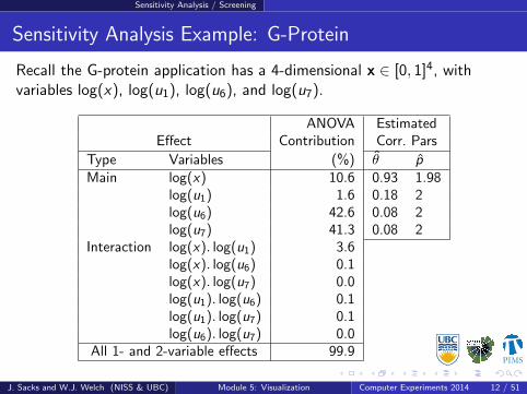
Sensitivity Analysis Example: G-Protein
Recall the G-protein application has a 4-dimensional x ∈ [0, 1]4, withvariables log(x), log(u1), log(u6), and log(u7).
ANOVA EstimatedEffect Contribution Corr. Pars
Type Variables (%) θ pMain log(x) 10.6 0.93 1.98
log(u1) 1.6 0.18 2log(u6) 42.6 0.08 2log(u7) 41.3 0.08 2
Interaction log(x). log(u1) 3.6log(x). log(u6) 0.1log(x). log(u7) 0.0log(u1). log(u6) 0.1log(u1). log(u7) 0.1log(u6). log(u7) 0.0
All 1- and 2-variable effects 99.9
J. Sacks and W.J. Welch (NISS & UBC) Module 5: Visualization Computer Experiments 2014 12 / 51
2 2PIMS
..........
.....
.....................................................................
.....
......
.....
.....
.
Visualization
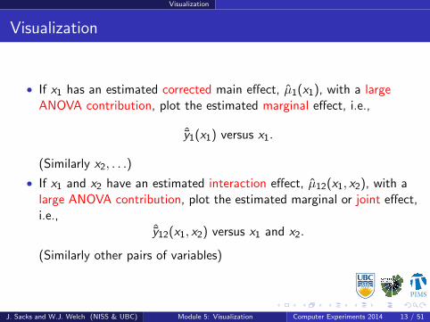
Visualization
• If x1 has an estimated corrected main effect, µ1(x1), with a largeANOVA contribution, plot the estimated marginal effect, i.e.,
ˆy1(x1) versus x1.
(Similarly x2, . . .)
• If x1 and x2 have an estimated interaction effect, µ12(x1, x2), with alarge ANOVA contribution, plot the estimated marginal or joint effect,i.e.,
ˆy12(x1, x2) versus x1 and x2.
(Similarly other pairs of variables)
J. Sacks and W.J. Welch (NISS & UBC) Module 5: Visualization Computer Experiments 2014 13 / 51

2 2PIMS
..........
.....
.....................................................................
.....
......
.....
.....
.
Visualization
Visualization Example: G-Protein
e.g., estimated main effects (lines) of log(u1) and log(u6) withapproximate 95% confidence limits (dashes)
0.0 0.2 0.4 0.6 0.8 1.0
0.2
0.3
0.4
0.5
0.6
logu1
yMod
yMod(logu1) : 1.6%
0.0 0.2 0.4 0.6 0.8 1.0
0.2
0.3
0.4
0.5
0.6
logu6
yMod
yMod(logu6) : 42.6%
J. Sacks and W.J. Welch (NISS & UBC) Module 5: Visualization Computer Experiments 2014 14 / 51

2 2PIMS
..........
.....
.....................................................................
.....
......
.....
.....
.
Visualization
Visualization Example: G-Protein
Similarly, log(u7) and log(x)
0.0 0.2 0.4 0.6 0.8 1.0
0.2
0.3
0.4
0.5
0.6
logu7
yMod
yMod(logu7) : 41.3%
0.0 0.2 0.4 0.6 0.8 1.0
0.2
0.3
0.4
0.5
0.6
logx
yMod
yMod(logx) : 10.6%
J. Sacks and W.J. Welch (NISS & UBC) Module 5: Visualization Computer Experiments 2014 15 / 51

2 2PIMS
..........
.....
.....................................................................
.....
......
.....
.....
.
Visualization
Main Effects: Comments
• log(u1) has a small estimated effect
• log(u6) and log(u7) have large, linear estimated effects
• log(x) appears to have a large, nonlinear effect.
• The estimated effect magnitudes are not obvious from the θ’s. Recall. . .
EstimatedANOVA % Corr. Pars
Main effect contribution θ plog(x) 10.6 0.93 1.98log(u1) 1.6 0.18 2log(u6) 42.6 0.08 2log(u7) 41.3 0.08 2
J. Sacks and W.J. Welch (NISS & UBC) Module 5: Visualization Computer Experiments 2014 16 / 51

2 2PIMS
..........
.....
.....................................................................
.....
......
.....
.....
.
Visualization
Estimated Joint Effect of log(u1) and log(x)
logu1
logx
0.0 0.2 0.4 0.6 0.8 1.0
0.0
0.2
0.4
0.6
0.8
1.0
yMod(logu1, logx) : 1.6+10.6+3.6=15.7%
logu1
logx
0.0 0.2 0.4 0.6 0.8 1.0
0.0
0.2
0.4
0.6
0.8
1.0
se[yMod(logu1, logx)]
J. Sacks and W.J. Welch (NISS & UBC) Module 5: Visualization Computer Experiments 2014 17 / 51

2 2PIMS
..........
.....
.....................................................................
.....
......
.....
.....
.
Visualization
Joint Effect of log(u1) and log(x): Comments
Based on the estimated effects, it appears that
• log(u1) has a small main effect
• log(x) has a large main effect.
But
• The log(u1)× log(x) interaction effect modifies the effect of log(x).
• In the joint effect plot (main effects plus interaction effect), log(x)has a much larger effect when log(u1) is small.
J. Sacks and W.J. Welch (NISS & UBC) Module 5: Visualization Computer Experiments 2014 18 / 51

2 2PIMS
..........
.....
.....................................................................
.....
......
.....
.....
.
Visualization
Computation of Effects and ANOVA
• We are decomposing the function y(x) and not the data from thecomputer model.
• The data are not necessarily from an orthogonal design.
• We are assuming that x is on a rectangular (orthogonal) space.
• (We can deal with some variables on a non-rectangular region.)
• Hence ANOVA of y(x) is mathematically possible.
• The high-dimensional integrals in the estimated effects and ANOVAare easy to compute if the correlation function has a product form (aswe usually take!).
J. Sacks and W.J. Welch (NISS & UBC) Module 5: Visualization Computer Experiments 2014 19 / 51

2 2PIMS
..........
.....
.....................................................................
.....
......
.....
.....
.
Case Study: Arctic Sea-Ice Computer Model
Arctic Sea-Ice Computer Model
• Purpose• Assess sensitivities to parameters such as drag coefficients, snowfall
rate, minimum lead fraction
• Model• Dynamic formulation based on a momentum balance for a mass of ice
within a grid cell• Model run: daily time step 1960-1988; 110 km grid covering Arctic
Ocean and nearby bodies of water
J. Sacks and W.J. Welch (NISS & UBC) Module 5: Visualization Computer Experiments 2014 20 / 51

2 2PIMS
..........
.....
.....................................................................
.....
......
.....
.....
.
Case Study: Arctic Sea-Ice Computer Model
Arctic Sea-Ice: Code Output
J. Sacks and W.J. Welch (NISS & UBC) Module 5: Visualization Computer Experiments 2014 21 / 51

2 2PIMS
..........
.....
.....................................................................
.....
......
.....
.....
.
Case Study: Arctic Sea-Ice Computer Model
Arctic Sea-Ice Variables
• Inputs (13 parameters)• Drag coefficients: AtmosDrag, OceanicDrag• Ice strength: LogIceStr• Minimum lead fraction: MinLead• Albedos: SnowAlbedo, IceAlbedo, OpenAlbedo• Exchange coefficient, surface sensible heat: SensHeat• Exchange coefficient, surface latent heat: LatentHeat• Snowfall rate: Snowfall• Cloud depletion of solar flux: Shortwave,• Cloud enhancement of longwave flux: Longwave• Oceanic heat flux: OceanicHeat
• Outputs (4 variables)• IceMass, IceArea, IceVelocity, RangeOfArea
J. Sacks and W.J. Welch (NISS & UBC) Module 5: Visualization Computer Experiments 2014 22 / 51

2 2PIMS
..........
.....
.....................................................................
.....
......
.....
.....
.
Case Study: Arctic Sea-Ice Computer Model
Experimental Design
• Initial 81-run zero-correlation Latin hypercube (69 good runs)
• Augmented by 110 runs using the maximin distance criterion (further88 good runs)
• 157 good runs of the code
J. Sacks and W.J. Welch (NISS & UBC) Module 5: Visualization Computer Experiments 2014 23 / 51

2 2PIMS
..........
.....
.....................................................................
.....
......
.....
.....
.
Case Study: Arctic Sea-Ice Computer Model
Experimental Design (First 3 Input Variables)
O
O
O
O
O
O
O
O
O
O
O
O
O
O
O
O
O
O
O
O
O
O
O
O
O
O
O
O
O
O
O
O
O
OO
O
O
O
O
O
O
O
O
O
O
O
O
O
O
OO
O
O
O
O
O
O
O
O
O
O
O
O
O
O
O
O
O
O
O
O
OO
O
O
O
O
O
OO O
O
O
O
O
O
O
O
O
O
O
O
O
O
O
O
O
O
O
O
O
O
O
O
O
O
O
O
O
O
O
O
O
O
O
O
O
O
O
O
O
O
O
OO
O
O
O
O
OO
O
O
O
O
O
O
O
O
O
O
OO
O
OO
O
O
O
O
O
O
O
O
O
OOO
O
O
O
O
O
O
O
O
O
O
O
O
O
O
OO
O
O
O
O
OO
O
O
O
O
O
O
O
O
O
O
O
SnowAlbedo
Sho
rtw
ave
0.50 0.75 1.00
1.0
2.5
4.0
O
O
O
O
O
O
O
O
O
O
O
O
OO
OO
O
OO O
O
OO
O
O
O
O
O
O
O
O
O
O
O
O
O
O
O
O
O
O
O
O
O
OO
O OO
O
O
O
O
O
O
O
O
O
O
O
O O
O
O
O
O
O
O OO
O
OO
O
OO
O
O
O
O
O
O
O
OO
OO
O
O
O
O
O
O
OO
O
OO
O
O
O
O
O
O
O
O
O
O
O
O
O
O
O
O
O
O
O
O
O
O
O
O
O
O
O
O
O
O
O
O
OO
OO
O
O
O
O
O
O
O
O
O
O
O
OO
O O
OO
O
O
O
O
O
O
O
O O
O
O
O
OO
O
O
O
O
O
O
O
O
O
O
O
O
O
O
O
O
O
O
O
O
O
O
O
O
O
O
SnowAlbedo
Min
Lead
0.50 0.75 1.00
0.00
0.03
0.06
O
O
O
O
O
O
O
O
O
O
O
O
OO
OO
O
OOO
O
OO
O
O
O
O
O
O
O
O
O
O
O
O
O
O
O
O
O
O
O
O
O
OO
O O O
O
O
O
O
O
O
O
O
O
O
O
O O
O
O
O
O
O
O OO
O
OO
O
OO
O
O
O
O
O
O
O
O O
OO
O
O
O
O
O
O
OO
O
OO
O
O
O
O
O
O
O
O
O
O
O
O
O
O
O
O
O
O
O
O
O
O
O
O
O
O
O
O
O
O
O
O
OO
OO
O
O
O
O
O
O
O
O
O
O
O
OO
OO
OO
O
O
O
O
O
O
O
OO
O
O
O
OO
O
O
O
O
O
O
O
O
O
O
O
O
O
O
O
O
O
O
O
O
O
O
O
O
O
O
Shortwave
Min
Lead
1.0 2.5 4.0
0.00
0.03
0.06
J. Sacks and W.J. Welch (NISS & UBC) Module 5: Visualization Computer Experiments 2014 24 / 51

2 2PIMS
..........
.....
.....................................................................
.....
......
.....
.....
.
Case Study: Arctic Sea-Ice Computer Model
Fitting the Gaussian Process (GP) Model
• Recall Gaussian process (GP) model for y(x):• y(x) at any x has mean µ and variance σ2
• µ is constant here (no trends)
• Cor(y(x), y(x′)) = R(x, x′) =∏d
j=1 exp(−θj |xj − x ′j |pj )• i.e., power-exponential with d = 13 here
• MLE to estimate µ, σ2, θ1, . . . , θ13, p1, . . . , p13• 28-dimensional optimization• Repeated for the 4 outputs• 10 maximum likelihood tries per output• Takes about 50 mins on a laptop• Many pj < 2
J. Sacks and W.J. Welch (NISS & UBC) Module 5: Visualization Computer Experiments 2014 25 / 51

2 2PIMS
..........
.....
.....................................................................
.....
......
.....
.....
.
Case Study: Arctic Sea-Ice Computer Model
Fitting the Gaussian Process (GP) Model
• Predict via y(x), the posterior mean (conditional on the data)
• Uncertainty of prediction from s(x) =√
v(x), i.e., from the posteriorvariance
• Check accuracy of y(x) and validity of s(x) via• Cross validated predictions, y−i (x(i))• Cross validated standard errors, s−i (x(i)).
• Show diagnostics and results for 2 outputs:• Ice area (moderately easy to predict)• Ice velocity (hard to predict)
J. Sacks and W.J. Welch (NISS & UBC) Module 5: Visualization Computer Experiments 2014 26 / 51

2 2PIMS
..........
.....
.....................................................................
.....
......
.....
.....
.
Case Study: Arctic Sea-Ice Computer Model
Diagnostics: Ice Area (✓)
o
o
o
o
oo
o
ooo
o
o
o
o
oo
oo
o
o o
oo
o
oo
oooo
o
o
o
o
o
o
o
o
o
oo
o
o
o
ooo
o
o
o
o
o
o
oo
o
o
o
o
oo
o
oo
o
o
o
o
o
o
o
o
o
o
o
o oo
o
o
o
o
o
o
o
o
o
o
o
o
oo
o
o
o
oo
o
o
o
o
o
o
o
o
o
o
o
o
o
oo
oooo
o
oo
ooo
o
o
o
o
o
o
oo
o
o
o
o
o oooo
o
o
o
o
ooooo
ooo
o
o
ooo
o
500 600 700 800 900 1000 1100
500
600
700
800
900
1000
1100
Predicted IceArea
IceA
rea
o
o
o
o oo
o
o
o
o
o
o
oo
o
o
oo
o o
o
o
o
oo
oo
o
o
oo
oo
o
o
o
o
o
oo
o
o
oo
o
o
o
oooo
o
o
oo
o
oo
o
o
o
o
o
o
o
o
o
o
o
o
o
o
oo
o
o
o
oo o
o
oo
o
oo
o
o
o
o
o o
o
o
oo
oo
o
o
o
o
ooo o
oo
o o
oo
ooo
oo
o o
o
oo
oo
o
oo
o
oo
o
o
o
o
o
oo
o
o
o
o
o
o
oo
oo
o oo
ooo
o
o
o
o
500 600 700 800 900 1000 1100
−4
−2
02
4
Predicted IceArea
Sta
ndar
dize
d re
sidu
al
J. Sacks and W.J. Welch (NISS & UBC) Module 5: Visualization Computer Experiments 2014 27 / 51

2 2PIMS
..........
.....
.....................................................................
.....
......
.....
.....
.
Case Study: Arctic Sea-Ice Computer Model
Diagnostics: Ice Velocity (×)
oo
o
o
o
o
oo
o
o
o
o
o
o
o
o
o
o
o
o
o
o
o
o
o
o
o
o
o
o
o
oo
o
o
o
o
o
o
o o
o
o
oo
o
o
oo
o
o
o
o
o
oo
o
o
o
o
o
o
o
o
o
oo
o
o
o
o
o
o
o
o
o
o
o
o
o
o
oo
o
o
o
o
o
o
o
o
o
o
o
o
o
o
o
o
o
o
o
o
o
o
oo
o
o
oo
o
o
o
o
o
o
o
o
o
oo
o
o
o
o
o
o
o
o
o
oo
o
o
oo
o
o
o
o
o
o
o
o
o
o
o
o
o
o
o
ooo
o
o
0 20 40 60 80 100
020
4060
8010
0
Predicted IceVelocity
IceV
eloc
ity o
oo
o
o
o
o
ooo
o
o
o
o
o
oo
o
o
o
ooo
oo
o
oo ooo
o
oo
o
o o
o
o
o
o o
o
o
o
o
o
oo
o
o o
o
ooo
o
oo
o
o
o
o
o
o
o
o
ooo
o
o
oooo
oo
o
o
o
o
o
o
o
o
o
o
o
o
o
o
o
o
oo
oo
o
o
o
o
o
oo
oo
oo
o
o
o
o
o o
o
o
o
o
o
o
o
ooo
oo
o
o
o
o o
oo
o
oo
o
o
o
oo
o
o
o
o
o
o
o
o
o
o
o
ooo
o
0 20 40 60 80 100
−4
−2
02
4
Predicted IceVelocity
Sta
ndar
dize
d re
sidu
al
J. Sacks and W.J. Welch (NISS & UBC) Module 5: Visualization Computer Experiments 2014 28 / 51

2 2PIMS
..........
.....
.....................................................................
.....
......
.....
.....
.
Case Study: Arctic Sea-Ice Computer Model
Comments
Ice area
• Accuracy moderately good
• Standard errors are fairly valid
Ice velocity
• Accuracy not so good
• Standard errors are invalid (5 standardized residuals outside ±3)
J. Sacks and W.J. Welch (NISS & UBC) Module 5: Visualization Computer Experiments 2014 29 / 51
2 2PIMS
..........
.....
.....................................................................
.....
......
.....
.....
.
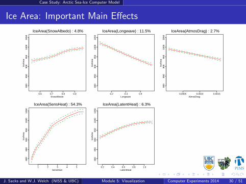
Case Study: Arctic Sea-Ice Computer Model
Ice Area: Important Main Effects
0.6 0.7 0.8 0.9
800
850
900
950
1000
1050
SnowAlbedo
IceA
rea
IceArea(SnowAlbedo) : 4.8%
0.2 0.3 0.480
085
090
095
010
0010
50Longwave
IceA
rea
IceArea(Longwave) : 11.5%
0.0005 0.0010 0.0015
800
850
900
950
1000
1050
AtmosDrag
IceA
rea
IceArea(AtmosDrag) : 2.7%
1 2 3 4 5
800
850
900
950
1000
1050
SensHeat
IceA
rea
IceArea(SensHeat) : 54.3%
0.2 0.4 0.6 0.8 1.0
800
850
900
950
1000
1050
LatentHeat
IceA
rea
IceArea(LatentHeat) : 6.3%
J. Sacks and W.J. Welch (NISS & UBC) Module 5: Visualization Computer Experiments 2014 30 / 51

2 2PIMS
..........
.....
.....................................................................
.....
......
.....
.....
.
Case Study: Arctic Sea-Ice Computer Model
Ice Area Main Effects: Comments
• The error bars are approximate pointwise 95% confidence intervals.
• SensHeat has a strong and moderately nonlinear estimated effect.• SensHeat also appears in an estimated interaction effect with
LatentHeat• The interaction effect accounts for another 4% of the variation, so plot
the corresponding joint effect (overall mean + main effects +interaction effect) . . .
J. Sacks and W.J. Welch (NISS & UBC) Module 5: Visualization Computer Experiments 2014 31 / 51

2 2PIMS
..........
.....
.....................................................................
.....
......
.....
.....
.
Case Study: Arctic Sea-Ice Computer Model
Ice Area: Important Interaction Effect
SensHeat
Late
ntH
eat
700 750
800 850
900
950 1000
1050
1 2 3 4 5
0.2
0.4
0.6
0.8
1.0
J. Sacks and W.J. Welch (NISS & UBC) Module 5: Visualization Computer Experiments 2014 32 / 51

2 2PIMS
..........
.....
.....................................................................
.....
......
.....
.....
.
Case Study: Arctic Sea-Ice Computer Model
Ice Velocity: Important Main Effects
0.01 0.02 0.03 0.04 0.05
2040
6080
100
MinLead
IceV
eloc
ity
IceVelocity(MinLead) : 7.7%
0.0005 0.0010 0.001520
4060
8010
0AtmosDrag
IceV
eloc
ity
IceVelocity(AtmosDrag) : 27.6%
1 2 3 4 5
2040
6080
100
SensHeat
IceV
eloc
ity
IceVelocity(SensHeat) : 2.9%
3.5 4.0 4.5 5.0
2040
6080
100
LogIceStr
IceV
eloc
ity
IceVelocity(LogIceStr) : 3.2%
2 4 6 8
2040
6080
100
OceanicDrag
IceV
eloc
ity
IceVelocity(OceanicDrag) : 45.5%
J. Sacks and W.J. Welch (NISS & UBC) Module 5: Visualization Computer Experiments 2014 33 / 51

2 2PIMS
..........
.....
.....................................................................
.....
......
.....
.....
.
Case Study: Arctic Sea-Ice Computer Model
Ice Velocity Main Effects: Comments
AtmosDrag and OceanicDrag have strong, nonlinear estimated effects.
• These 2 inputs also have a modest interaction effects, accounting foranother 4% of the variation
• So plot the corresponding joint effect (overall mean + main effects +interaction effect) . . .
J. Sacks and W.J. Welch (NISS & UBC) Module 5: Visualization Computer Experiments 2014 34 / 51

2 2PIMS
..........
.....
.....................................................................
.....
......
.....
.....
.
Case Study: Arctic Sea-Ice Computer Model
Ice Velocity: Important Interaction Effect
AtmosDrag
Oce
anic
Dra
g
20
20
30
40
50
60
70 80 90
100 110
0.5 1.0 1.5
24
68
J. Sacks and W.J. Welch (NISS & UBC) Module 5: Visualization Computer Experiments 2014 35 / 51

2 2PIMS
..........
.....
.....................................................................
.....
......
.....
.....
.
Summary
Module Summary
• Define the scientific problem in terms of y(x) (if it could be computedmany times cheaply)
• Replace y(x) by y(x).
• ANOVA decomposes the variability in y(x) to identify important mainand interaction effects.
• Important effects can be visualized by plotting.
• Sensitivity analysis, optimization, propagation of variation, . . . arefeasible using y(x) for fairly large problems.
J. Sacks and W.J. Welch (NISS & UBC) Module 5: Visualization Computer Experiments 2014 36 / 51

2 2PIMS
..........
.....
.....................................................................
.....
......
.....
.....
.
Case Study: Wonderland Computer Model
Wonderland Computer Model
• Lempert et al. (2003), “Shaping the Next One Hundred Years . . .,”RAND, http://www.rand.org/publications/MR/MR1626/
• Visualization / sensitivity analysis example in Schonlau and Welch(2006)
• Wonderland can model various global economic/environmentalscenarios.
• Here, we model a “limits to growth” policy, where carbon taxes areset high enough for zero growth in emissions after 2010.
• The objective is to understand the input-output relationship:sensitivity analysis and visualization.
J. Sacks and W.J. Welch (NISS & UBC) Module 5: Visualization Computer Experiments 2014 37 / 51

2 2PIMS
..........
.....
.....................................................................
.....
......
.....
.....
.
Case Study: Wonderland Computer Model
Wonderland Variables
• 41 Input variables relating to• population growth• economic activity• changes in environmental conditions• other economic and demographic variables
• Output variable, HDI, (bigger is better) is a quasi global humandevelopment index, relating to
• net output per capita• death rates• flow of pollutants, etc.
J. Sacks and W.J. Welch (NISS & UBC) Module 5: Visualization Computer Experiments 2014 38 / 51

2 2PIMS
..........
.....
.....................................................................
.....
......
.....
.....
.
Case Study: Wonderland Computer Model
Important (We See Later) Input Variables
Variable Description
e.finit Flatness of initial decline in economic growthe.grth Base economic growth ratee.inov Innovation ratee.cinov Effect of innovation policies (pollution taxes) on growthv.spoll Sustainable pollutionv.cfsus Change in level of sustainable pollution when natural cap-
ital is cut in halfv.drop Rate of drop in natural capital when pollution flows are
above the sustainable level
• Most variables are really two variables: north and south versions• Sometimes both are important, e.g., e.inov.n and e.inov.s• Sometimes only one is important, e.g., v.spoll.s
J. Sacks and W.J. Welch (NISS & UBC) Module 5: Visualization Computer Experiments 2014 39 / 51

2 2PIMS
..........
.....
.....................................................................
.....
......
.....
.....
.
Case Study: Wonderland Computer Model
Experimental Design: 500-run Latin hypercube in 41-D
First 2 input variables
0.00 0.01 0.02 0.03 0.04
−0.
010.
000.
010.
020.
030.
040.
05
e.grth.n
e.in
ov.n
J. Sacks and W.J. Welch (NISS & UBC) Module 5: Visualization Computer Experiments 2014 40 / 51

2 2PIMS
..........
.....
.....................................................................
.....
......
.....
.....
.
Case Study: Wonderland Computer Model
Raw Data
Plot HDI against two of the input variables (later shown to be important)
−0.01 0.00 0.01 0.02 0.03 0.04 0.05
−0.
4−
0.3
−0.
2−
0.1
0.0
e.inov.n
HD
I
0 2 4 6 8 10
−0.
4−
0.3
−0.
2−
0.1
0.0
v.spoll.s
HD
I
J. Sacks and W.J. Welch (NISS & UBC) Module 5: Visualization Computer Experiments 2014 41 / 51

2 2PIMS
..........
.....
.....................................................................
.....
......
.....
.....
.
Case Study: Wonderland Computer Model
Gaussian Process (GP) Model
• Recall Gaussian process (GP) model for y(x):• y(x) at any x has mean µ and variance σ2
• Cor(y(x), y(x′)) = R(x, x′) =∏d
j=1 exp(−θj |xj − x ′j |pj ), with d = 41here
• MLE to estimate µ, σ2, θ1, . . . , θ41, p1, . . . , p41• 84-dimensional optimization• Takes < 1 hour on a laptop• Many pj < 2
• Predict via y(x), the posterior mean (conditional on the data)
• Uncertainty of prediction from s(x) =√
v(x), i.e., from the posteriorvariance
• Check accuracy of y(x) and validity of s(x) via cross validatedpredictions, y−i (x
(i)), and cross validated standard errors, s−i (x(i)).
J. Sacks and W.J. Welch (NISS & UBC) Module 5: Visualization Computer Experiments 2014 42 / 51

2 2PIMS
..........
.....
.....................................................................
.....
......
.....
.....
.
Case Study: Wonderland Computer Model
Gaussian Process Model Diagnostics
oo
o
o
o
o
o
oo
o
ooo
oo
o
o
oo
ooo
o
o
ooo
oo
oo
oo
o oooo
o
o
oo
o
ooo
o
o
o
oo
o o
oo
o o
o
o oo
oo
oo
oooo
o
o
oo
oo
o
o
o o
o
o
ooo
o
o
oo
o
o
o
o
ooo oo
o
o
oo
o
o
o
o
o
o o
o oo
o
oo
oo
oo
ooo
o
o
oo o
o
oo
o
oo o
oo
o
oooo
o
o
oo
o
oo
o
o
oo
o
o o
oo
oo
o
o oooo
oo
o
o o
oo
o
o oooo
o
o
o
o
oooo
o o
oo
o
o
o
o
oo
ooo
o
o
ooo
ooo
oo
oo
o
o o
o
o
o
oo
o oo
oo
o
o
oo
oo
oooo
o
oo
o
o
ooo
oo
o
ooo
o
o
o
oo
o
oo
oo oo
o
o
o
o
o
o
o
o
o
o
oo
o
oooo
o
o
oo
oo
o
ooo
o
oo
o
o
o
oo
oo
ooooo
oo
oo
oo o
o
oooo
oo
oooo
o
oo
o
ooo
o oo
o
o
oo
o
o
oo oo
oo
o
o
o
oo
oo o
o
o
oo
o
o
oo
oo
oo
o
o o
oo
o
o
o
oo
o
ooo
ooo
o
o
oo
ooo oo
o
o
oo
o
o
o o
o
o
o
o
ooo
oo
ooo
oooo
o
o
oo
o
o
ooo
o
ooo
ooo
ooo
oo o
ooo
oo
oo o
ooo
o
o
o
ooo
o
o
o
o
o
o
o o
o
oo ooo
ooo
o
o
o
ooo
oo oo
o
o
o oo
o
oo
o
oo
o
o
o o
oo
oo
oo
o
o
−0.4 −0.3 −0.2 −0.1 0.0
−0.
4−
0.3
−0.
2−
0.1
0.0
Predicted HDI
HD
I
o oo
o
o
oo
oo
o
oo
o
o
oo
o
oo
oo
oo
o o
oo
o
o o oo
o
o
ooo
o
o
o
oo
o
oo
o
o
o
oo
oo
o
o
oo
oo
o
oo
o
o
o
o o
oo
o o
o
o
o o
o
o
oo
o
oo
o
oo oo
ooo
oo
oo
o
o
oo
o
o
o
o
o
o
o o
o
o
o
o
o
o
o o
oo
o
o
o
oo
o
o
o
o
o
oo
o
o
o
o
o
o
o
oo oo
oo
o
o
o
o
o
oo
o
o
o
o
o
o
o
o
o o
oo
oo
o oo
o
o
oo
oo
oo
o
oo
o
o
o
o
o
o
o
o
o
o
o
oo o
oo
o
o
oo
o
o
oo
o
o
oo
o
o
ooo
ooo
o
o
o
o
o
o
o
o
o
ooo o
oo
o
o o
o
oo
o
o
oo
o
o
o
o
oo
o
o
o
o
oo
o
o
o
o
o
oo o
o
oo
o
o
o
o
o
oo
o oo
o
o
oo
oo
oo
o
o
oo
o
o
o
oo
o
o
o
oo
oo
o
oo
oo
oo
o
o
oo
oo
o
oo
oo o
o
ooo
o
o
o
o
o
o
o
oooo
o
o
o
o
o
o
o
o
ooo
o
o
ooo
o
o
o o
o
ooo
oo
o
oo
o
o
o
oo
o
o
o
oo
o
oo oo
o
o
o
o
o
o
oo
o
o
o
o o
o
o
oo o
o
o
o
o
o
o
o
o
o
o
o
o
o
o
o
o
oo
oooo
o
o
o
o
o
o
o
oo
o
o
o
oo
oo
ooooo
oo
o
oo
o
o
o
o
ooo
o
o
o
ooo
o
o
oo
o
o
o
oo
oo
oo
o
ooo
o
oo
o
oo
oo
oo
o
o
o
o
o
o
o
oo o
ooo
o
o
o
o
o
oo
o
oo
−0.3 −0.2 −0.1 0.0
−4
−2
02
4
Predicted HDI
Sta
ndar
dize
d re
sidu
al
J. Sacks and W.J. Welch (NISS & UBC) Module 5: Visualization Computer Experiments 2014 43 / 51

2 2PIMS
..........
.....
.....................................................................
.....
......
.....
.....
.
Case Study: Wonderland Computer Model
Cross Validation: Numerical Summary of Accuracy
Recall, the cross validated error is
y(x(i))− y−i (x(i))
• Cross-validate root mean squared error (CVRMSE) is 0.026
• Fairly accurate relative to a range of about 0.5 in y
• But maximum error is 0.198: the few extremely low values of y arenot predicted well when removed from the data under cross validation.
J. Sacks and W.J. Welch (NISS & UBC) Module 5: Visualization Computer Experiments 2014 44 / 51

2 2PIMS
..........
.....
.....................................................................
.....
......
.....
.....
.
Case Study: Wonderland Computer Model
Cross Validation: Standard errors?
• Cross validated errorStandard error
is mainly in (−2, 2).
• But 7/500 are outside (−3, 3) and 2/500 are outside (−4, 4).
• Standard errors are fairly reliable but sometimes underestimated here.
J. Sacks and W.J. Welch (NISS & UBC) Module 5: Visualization Computer Experiments 2014 45 / 51

2 2PIMS
..........
.....
.....................................................................
.....
......
.....
.....
.
Case Study: Wonderland Computer Model
Comment
• Visualization will show that y(x) is extremely nonlinear, possiblynonstationary, and hence difficult to model.
• Other methods will face the same difficulties.
J. Sacks and W.J. Welch (NISS & UBC) Module 5: Visualization Computer Experiments 2014 46 / 51

2 2PIMS
..........
.....
.....................................................................
.....
......
.....
.....
.
Case Study: Wonderland Computer Model
Sensitivity Analysis: Functional ANOVA (of GP Predictor)
• 41 main effects
• 820 2-factor interaction effects!
• Estimated effects accounting for > 1% of the variability in y(x)(involving 8 input variables)
% of total % of totalEffect variance Effect variance
e.inov.n 24.3 v.spoll.s × v.drop.s 2.7v.spoll.s 13.5 e.grth.n × e.inov.n 1.9e.inov.s 12.1 v.drop.s 1.9e.cinov.s 5.3 e.finit.s 1.5v.spoll.s × v.cfsus.s 4.6 e.inov.n × e.inov.s 1.4v.drop.s × v.cfsus.s 3.7 v.cfsus.s 1.2
J. Sacks and W.J. Welch (NISS & UBC) Module 5: Visualization Computer Experiments 2014 47 / 51
2 2PIMS
..........
.....
.....................................................................
.....
......
.....
.....
.
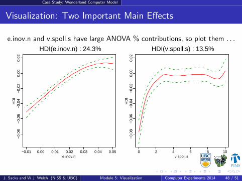
Case Study: Wonderland Computer Model
Visualization: Two Important Main Effects
e.inov.n and v.spoll.s have large ANOVA % contributions, so plot them . . .
−0.01 0.00 0.01 0.02 0.03 0.04 0.05
−0.
08−
0.06
−0.
04−
0.02
0.00
0.02
e.inov.n
HD
I
HDI(e.inov.n) : 24.3%
0 2 4 6 8 10
−0.
08−
0.06
−0.
04−
0.02
0.00
0.02
v.spoll.s
HD
I
HDI(v.spoll.s) : 13.5%
J. Sacks and W.J. Welch (NISS & UBC) Module 5: Visualization Computer Experiments 2014 48 / 51

2 2PIMS
..........
.....
.....................................................................
.....
......
.....
.....
.
Case Study: Wonderland Computer Model
Main Effects: Comments
• The error bars are approximate pointwise 95% confidence intervals.
• v.spoll.s has a very nonlinear estimated effect.• But it has several large estimated interaction effects.• e.g., estimated v.spoll.s × v.cfsus.s interaction effect accounts for
nearly 5% of the variation, so plot the corresponding joint effect(overall mean + main effects + interaction effect) . . .
J. Sacks and W.J. Welch (NISS & UBC) Module 5: Visualization Computer Experiments 2014 49 / 51

2 2PIMS
..........
.....
.....................................................................
.....
......
.....
.....
.
Case Study: Wonderland Computer Model
Estimated Joint Effect of v.spoll.s and v.cfsus.s
v.spoll.s
v.cf
sus.
s
0 2 4 6 8 10
0.6
0.8
1.0
1.2
HDI(v.spoll.s, v.cfsus.s) : 13.5+1.2+4.6=19.3%
v.spoll.s
v.cf
sus.
s
0 2 4 6 8 10
0.6
0.8
1.0
1.2
se[HDI(v.spoll.s, v.cfsus.s)]
J. Sacks and W.J. Welch (NISS & UBC) Module 5: Visualization Computer Experiments 2014 50 / 51

2 2PIMS
..........
.....
.....................................................................
.....
......
.....
.....
.
Case Study: Wonderland Computer Model
Joint Effect of v.vspoll.s and v.cfsus.s: Comments
Based on the estimated effects, it appears that
• v.spoll.s has a large main effect and v.cfsus.s has a small main effect
• The v.spoll.s× v.cfsus.s interaction effect modifies the effect ofv.vspoll.s.
• In the joint effect plot (main effects plus interaction effect), v.vspoll.shas a much larger effect when v.cfsus.s is large.
• Small v.vspoll.s and large v.cfsus.s give bad (catastrophic?) estimatedHDI.
• The other large estimated interaction effects should be similarlyexamined.
J. Sacks and W.J. Welch (NISS & UBC) Module 5: Visualization Computer Experiments 2014 51 / 51