module 4f2: nonlinear systems and control · module 4f2: nonlinear systems and control lectures 1...
TRANSCRIPT

Module 4F2: NonlinearSystems and Control
Lectures 1 – 2: Dynamical Systems
Department of Engineering
University of Cambridge
Lent 2011 4F2: Nonlinear Systems and Control, Lectures 1–2 – p. 1/26

‘Nonlinear’ overview — 7LNonlinear dynamical systems 2 lectures
Continuous, discrete, hybrid
Examples
State-space description
Solutions, simulations
Attractors, Stability, Lyapunov methods 1.5 lectures
Describing functions 1.5 lectures
Circle criterion for stability 2 lectures
2 Examples papers, 1 Examples class
Lent 2011 4F2: Nonlinear Systems and Control, Lectures 1–2 – p. 2/26

Dynamical system classificationDynamical system:Evolution of state over time.
Types of state:
Continuous Statex lives in Euclidean spaceRn — familiar, eg
from 3F2. Writex ∈ Rn.
Discrete Stateq takes values in finite or countable set
{q1, q2, . . .}. Example: Light switch,q ∈ {ON,OFF}.
Hybrid Part of state lives inRn, other part has values in finite
set.Example: Computer control of inverted pendulum.
Lent 2011 4F2: Nonlinear Systems and Control, Lectures 1–2 – p. 3/26

Types of time:
Continuous x = Ax (linear) orx = f(x) (nonlinear).
Discrete xk+1 = Axk (linear) orxk+1 = f(xk) (nonlinear).
Hybrid System evolves over continuous time, but special things
happen at particular instants.
We will deal mostly with:
Continuous-state, continuous-time, nonlinear
Lent 2011 4F2: Nonlinear Systems and Control, Lectures 1–2 – p. 4/26
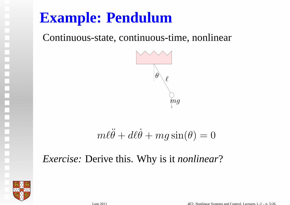
Example: PendulumContinuous-state, continuous-time, nonlinear
ℓθ
mg
mℓθ + dℓθ +mg sin(θ) = 0
Exercise: Derive this. Why is itnonlinear?
Lent 2011 4F2: Nonlinear Systems and Control, Lectures 1–2 – p. 5/26

Solve the ODE:Find
θ(·) : R → R
such that
θ(0) = θ0
θ(0) = θ0
mℓθ(t) + dℓθ(t) +mg sin(θ(t)) = 0, ∀t ∈ R
Usually difficult to find solution analytically.Find approximate solution bysimulation.
Lent 2011 4F2: Nonlinear Systems and Control, Lectures 1–2 – p. 6/26
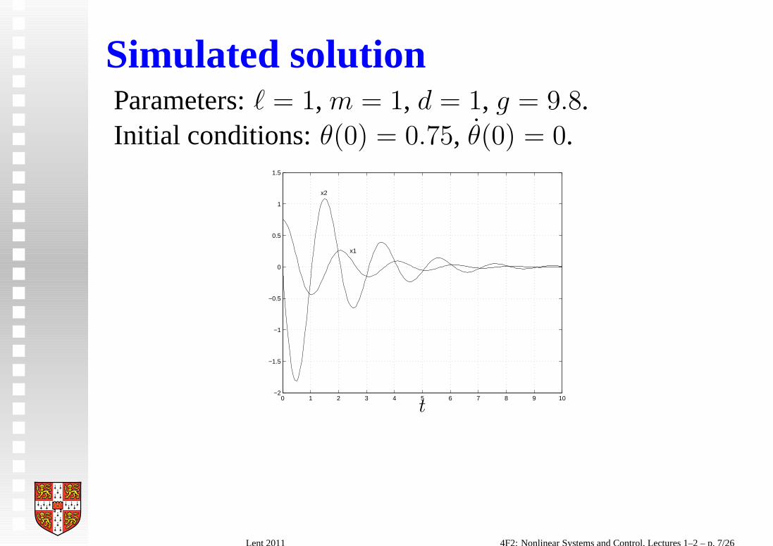
Simulated solutionParameters:ℓ = 1, m = 1, d = 1, g = 9.8.Initial conditions:θ(0) = 0.75, θ(0) = 0.
0 1 2 3 4 5 6 7 8 9 10−2
−1.5
−1
−0.5
0
0.5
1
1.5
x2
x1
t
Lent 2011 4F2: Nonlinear Systems and Control, Lectures 1–2 – p. 7/26

State-space form:
x = f(x), x ∈ Rn, n ≥ 1
For the pendulum,x ∈ R2:
x =
[x1x2
]
=
[θ
θ
]
which gives:
x =
[x1x2
]
=
[x2
−gℓ sin(x1)− d
mx2
]
= f(x)
x is state. This system hasdimension2.
Lent 2011 4F2: Nonlinear Systems and Control, Lectures 1–2 – p. 8/26

Vector field
x = f(x), f(·) : R2 → R2 is vector field
f(·) assignsvelocity vector to each state vector.
−0.25 −0.2 −0.15 −0.1 −0.05 0 0.05 0.1 0.15 0.2 0.25−0.6
−0.4
−0.2
0
0.2
0.4
0.6
θ
θ
Lent 2011 4F2: Nonlinear Systems and Control, Lectures 1–2 – p. 9/26

Solve the ODE (another view):Findx(·) : R → R
2 such that
x(0) =
[x1(0)
x2(0)
]
=
[θ0
θ0
]
x(t) = f(x(t)), ∀t ∈ R.
−0.6 −0.4 −0.2 0 0.2 0.4 0.6 0.8−2
−1.5
−1
−0.5
0
0.5
1
1.5
θ
θ
Lent 2011 4F2: Nonlinear Systems and Control, Lectures 1–2 – p. 10/26

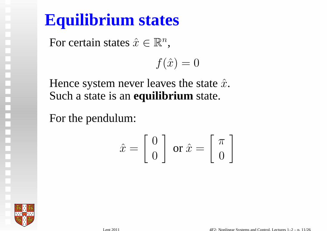
Equilibrium statesFor certain statesx ∈ R
n,
f(x) = 0
Hence system never leaves the statex.Such a state is anequilibrium state.
Lent 2011 4F2: Nonlinear Systems and Control, Lectures 1–2 – p. 11/26
Equilibrium statesFor certain statesx ∈ R
n,
f(x) = 0
Hence system never leaves the statex.Such a state is anequilibrium state.
For the pendulum:
x =
[0
0
]
or x =
[π
0
]
Lent 2011 4F2: Nonlinear Systems and Control, Lectures 1–2 – p. 11/26

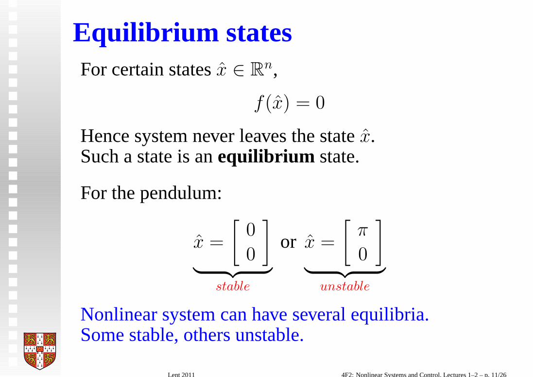
Equilibrium statesFor certain statesx ∈ R
n,
f(x) = 0
Hence system never leaves the statex.Such a state is anequilibrium state.
For the pendulum:
x =
[0
0
]
︸ ︷︷ ︸
stable
or x =
[π
0
]
︸ ︷︷ ︸
unstable
Lent 2011 4F2: Nonlinear Systems and Control, Lectures 1–2 – p. 11/26
Equilibrium statesFor certain statesx ∈ R
n,
f(x) = 0
Hence system never leaves the statex.Such a state is anequilibrium state.
For the pendulum:
x =
[0
0
]
︸ ︷︷ ︸
stable
or x =
[π
0
]
︸ ︷︷ ︸
unstable
Nonlinear system can have several equilibria.Some stable, others unstable.
Lent 2011 4F2: Nonlinear Systems and Control, Lectures 1–2 – p. 11/26

LinearisationForθ close to 0:sin(θ) ≈ θ. Hence forθ close to 0:
mℓθ + dℓθ +mgθ = 0
or in state space form
x =
[x2
−gℓx1 − d
mx2
]
=
[0 1
−gℓ − d
m
] [x1x2
]
= g(x)
Note thatg(x) = Ax ie linearstate-space system.A has eigenvalues in LHP — stable linear system.
Lent 2011 4F2: Nonlinear Systems and Control, Lectures 1–2 – p. 12/26

LinearisationForθ close to 0:sin(θ) ≈ θ. Hence forθ close to 0:
mℓθ + dℓθ +mgθ = 0
or in state space form
x =
[x2
−gℓx1 − d
mx2
]
=
[0 1
−gℓ − d
m
] [x1x2
]
= g(x)
Note thatg(x) = Ax ie linearstate-space system.A has eigenvalues in LHP — stable linear system.
Exercise: Find linearisation near the otherequilibrium. Examine its stability.
Lent 2011 4F2: Nonlinear Systems and Control, Lectures 1–2 – p. 12/26

Example: Logistic mapContinuous-state, discrete-time, nonlinear.
xk+1 = axk(1− xk) = f(xk)
Lent 2011 4F2: Nonlinear Systems and Control, Lectures 1–2 – p. 13/26

Example: Logistic mapContinuous-state, discrete-time, nonlinear.
xk+1 = axk(1− xk) = f(xk)
0 0.1 0.2 0.3 0.4 0.5 0.6 0.7 0.8 0.9 10
0.1
0.2
0.3
0.4
0.5
0.6
0.7
0.8
0.9
1
f(x)
x
Lent 2011 4F2: Nonlinear Systems and Control, Lectures 1–2 – p. 13/26

Equilibrium, Oscillation, Chaos
0 5 10 15 20 25 300
0.01
0.02
0.03
0.04
0.05
0.06
0.07
0.08
0.09
0.1a=0.9
0 ≤ a < 1: Decays to 0 for allx0. a = 0.9
Lent 2011 4F2: Nonlinear Systems and Control, Lectures 1–2 – p. 14/26

Equilibrium, Oscillation, Chaos
0 5 10 15 20 25 300
0.05
0.1
0.15
0.2
0.25
0.3
0.35
0.4
0.45
0.5a=2.0
1 ≤ a ≤ 3: Tends to steady-state value. a = 2.0
Lent 2011 4F2: Nonlinear Systems and Control, Lectures 1–2 – p. 14/26

Equilibrium, Oscillation, Chaos
0 5 10 15 20 25 300
0.1
0.2
0.3
0.4
0.5
0.6
0.7
0.8a=2.9
1 ≤ a ≤ 3: Tends to steady-state value. a = 2.9
Lent 2011 4F2: Nonlinear Systems and Control, Lectures 1–2 – p. 14/26

Equilibrium, Oscillation, Chaos
0 5 10 15 20 25 300
0.1
0.2
0.3
0.4
0.5
0.6
0.7
0.8a=3.2
3 < a ≤ 1 +√6 = 3.449:
Tends to 2-period oscillation. a = 3.2
Lent 2011 4F2: Nonlinear Systems and Control, Lectures 1–2 – p. 14/26

Equilibrium, Oscillation, Chaos
0 5 10 15 20 25 300
0.1
0.2
0.3
0.4
0.5
0.6
0.7
0.8
0.9
1a=3.8
1 +√6 < a < 4:
3-period, 4-period, . . . , chaos. a = 3.8
Lent 2011 4F2: Nonlinear Systems and Control, Lectures 1–2 – p. 14/26

Example: Manufacturing cell
A discrete-state system.
Possible states: Idle (I), Working (W), Down (D).
Possible events:p part arrivesc complete processingf failurer repair
Lent 2011 4F2: Nonlinear Systems and Control, Lectures 1–2 – p. 15/26

Abstract description of machine
q ∈ Q = {I,W,D}, σ ∈ Σ = {p, c, f, r}State transition relation:
δ : Q× Σ → Q
δ(I, p) = W , δ(W, c) = I, δ(W, f) = D, δ(D, r) = I.
Lent 2011 4F2: Nonlinear Systems and Control, Lectures 1–2 – p. 16/26

Abstract description of machine
q ∈ Q = {I,W,D}, σ ∈ Σ = {p, c, f, r}State transition relation:
δ : Q× Σ → Q
δ(I, p) = W , δ(W, c) = I, δ(W, f) = D, δ(D, r) = I.
Otherwiseδ is undefined — egδ(D, p).
Lent 2011 4F2: Nonlinear Systems and Control, Lectures 1–2 – p. 16/26

Abstract description of machine
q ∈ Q = {I,W,D}, σ ∈ Σ = {p, c, f, r}State transition relation:
δ : Q× Σ → Q
δ(I, p) = W , δ(W, c) = I, δ(W, f) = D, δ(D, r) = I.
Otherwiseδ is undefined — egδ(D, p).
f
c
rp
W D
I
Lent 2011 4F2: Nonlinear Systems and Control, Lectures 1–2 – p. 16/26

Example: ThermostatA hybrid system.
x ∈ R: Room temperature,q ∈ {ON,OFF}: Heater state.
Heater off: q = OFF , x = −ax
Heater on: q = ON , x = −a(x− 30)
Use hysteresis to prevent ‘chattering’:if x<19, q := ON,elseif x>21, q := OFF,end
Lent 2011 4F2: Nonlinear Systems and Control, Lectures 1–2 – p. 17/26

x22
21
20
19
18
t
Lent 2011 4F2: Nonlinear Systems and Control, Lectures 1–2 – p. 18/26

x22
21
20
19
18
t
OFF ON
x = −ax x = −a(x− 30)
x ≥ 18 x ≤ 22
x ≤ 19
x ≥ 21
Lent 2011 4F2: Nonlinear Systems and Control, Lectures 1–2 – p. 18/26

State-space formStates:xi ∈ R, i = 1, 2, . . . , nInputs: uj ∈ R,j = 1, 2, . . . ,mOutputs: yk ∈ R, k = 1, 2, . . . , p
x = f(x, u, t), y = h(u, x, t), vector functions
Special case:x = f(x) autonomous
Lent 2011 4F2: Nonlinear Systems and Control, Lectures 1–2 – p. 19/26

What dox = f(x, u, t) andy = h(u, x, t) mean?
x1 = f1(x1, . . . , xn, u1, . . . , um, t)...
xn = fn(x1, . . . , xn, u1, . . . , um, t)
y1 = h1(x1, . . . , xn, u1, . . . , um, t)...
yp = hp(x1, . . . , xn, u1, . . . , um, t)
Lent 2011 4F2: Nonlinear Systems and Control, Lectures 1–2 – p. 20/26

Existence, Uniquenessx = −sign(x), x(0) = 0 — No solutions
Lent 2011 4F2: Nonlinear Systems and Control, Lectures 1–2 – p. 21/26

Existence, Uniquenessx = −sign(x), x(0) = 0 — No solutions
x = 3x2/3, x(0) = 0 — Multiple solutions
For anya ≥ 0, x(t) =
{(t− a)3 t ≥ a
0 t ≤ a
Lent 2011 4F2: Nonlinear Systems and Control, Lectures 1–2 – p. 21/26

Existence, Uniquenessx = −sign(x), x(0) = 0 — No solutions
x = 3x2/3, x(0) = 0 — Multiple solutions
For anya ≥ 0, x(t) =
{(t− a)3 t ≥ a
0 t ≤ a
x = 1 + x2, x(0) = 0 — Finite escape timeOne solution:x(t) = tan(t)
Lent 2011 4F2: Nonlinear Systems and Control, Lectures 1–2 – p. 21/26

Lipschitz continuityDefinition 1 A function f : Rn → R
n is Lipschitzcontinuousif ∃λ > 0 such that ∀x, x ∈ R
n
‖f(x)− f(x)‖ < λ‖x− x‖
Lent 2011 4F2: Nonlinear Systems and Control, Lectures 1–2 – p. 22/26

Lipschitz continuityDefinition 2 A function f : Rn → R
n is Lipschitzcontinuousif ∃λ > 0 such that ∀x, x ∈ R
n
‖f(x)− f(x)‖ < λ‖x− x‖
Theorem 2 (Existence & Uniqueness of Solutions)If f is Lipschitz continuous, then
x = f(x), x(0) = x0
has a unique solution x(·) : [0, T ] → Rn for all T ≥ 0
and all x0 ∈ Rn.
Lent 2011 4F2: Nonlinear Systems and Control, Lectures 1–2 – p. 22/26

SimulationTheorem 3 (Continuity with Initial State) Assumef is Lipschitz continuous with Lipschitz constant λ.Let x(·) : [0, T ] → R
n and x(·) : [0, T ] → Rn be
solutions to x = f(x) with x(0) = x0 and x(0) = x0,respectively. Then for all t ∈ [0, T ]
‖x(t)− x(t)‖ ≤ ‖x0 − x0‖eλt
“Solutions that start close, remain close.”This justifiessimulation.
Lent 2011 4F2: Nonlinear Systems and Control, Lectures 1–2 – p. 23/26

Pendulum simulation (Matlab)
x =
[x1x2
]
=
[x2
−gℓ sin(x1)− d
mx2
]
= f(x)
function [xdot] = pendulum(t,x)l = 1; m=1; d=1; g=9.8;xdot(1) = x(2);xdot(2) = -sin(x(1))*g/l-x(2)*d/m;
Lent 2011 4F2: Nonlinear Systems and Control, Lectures 1–2 – p. 24/26

>> x=[0.75 0];>> [T,X]=ode45(’pendulum’, [0 10], x’);>> plot(T,X);>> grid;
ode45is 4’th order Runge-Kutta integration function.
Exercise: Try this at home! (or in the DPO)
Lent 2011 4F2: Nonlinear Systems and Control, Lectures 1–2 – p. 25/26

Simulation toolsSimulink provides GUI front-end toMatlab.Other similar products available.
Pendulum:
1s
x2
1s
x1
Scope1
d/m
Gain1
g/l
Gain
sin(u)
Fcn
Lent 2011 4F2: Nonlinear Systems and Control, Lectures 1–2 – p. 26/26